Environmental Kuznets Curve for Water Quality Parameters at Global Level

Krishna P. Paudel1, C.-Y. Cynthia Lin, Mahesh Pandit

Corresponding Author:

Krishna P. Paudel, Department of Agricultural Economics and Agribusiness, Louisiana State

University (LSU) and LSU Agricultural Center, Baton Rouge, LA 70803, Email:

kpaudel@agcenter.lsu.edu

Selected Paper prepared for presentation at the Southern Agricultural Economics

Association (SAEA) Annual Meeting, Dallas, Texas, February 1-4, 2014.

Copyright 2014 by Madhav Regmi, Krishna Paudel and Deborah Williams. All rights reserved. Readers may make verbatim copies of this document for non‐commercial purposes by any means, provided that this copyright notice appears on all such copies.

1 Paudel and Pandit are associate professor and former doctoral student, respectively, in the Department of

Agricultural Economics and Agribusiness at Louisiana State University Baton Rouge, Louisiana. Lin is an

associate professor in the Department of Agricultural and Resource Economics at the University of California

at Davis.

Environmental Kuznets Curve for Water Quality Parameters at Global Level

Abstract

We examine the relationship between income and water pollutants using

country-level global water quality data over the period 1980 to 2012. We

include civil liberties and political rights in addition to income as explanatory

variables. We use recent advances in econometric techniques to address the

inclusion of continuous and discrete variables in nonparametric instrumental

variable regression models. Results indicate an inverted U-shape relationship

between income and pollution for one pollutant (lead) and a cubic shape for

three pollutants (nickel, mercury and arsenic). In general, we find that

improved civil liberties and political rights are correlated with better water

quality. By estimating a nonparametric relationship between political

variables and pollution and by accounting for the categorical nature of the

political variables, we are able to detect a nonlinear relationship between

political variables and pollution, which for some pollutants is an inverted U-

shaped curve.

Key Words: Binary variable, environmental Kuznets curve, nonparametric instrumental

variable regressions, water pollution

JEL Codes: Q53, C14

Environmental Kuznets Curve for Water Quality Parameters at Global Level

The environmental Kuznets curve (EKC) is a relationship between income and pollution

which is hypothesized to have an inverted U-shape. The idea of an inverted U-shaped

Kuznets curve stems from the Kuznets' work in income equality (Kuznets, 1955). The EKC

hypothesis states that as income increases, pollution goes up initially but when income is

high enough, pollution eventually declines. The income level at which pollution level is the

highest is called a turning point.

There exist numerous papers on the validity, application, and measurement of the

EKC (Azomahou et al., 2006; Carson, 2010). This is evident from the seminal work by

Grossman and Krueger (1995), as well as papers focusing specifically on air pollution (e.g.

Bruvoll and Medin, 2003; Deacon and Norman, 2006; Heerink et al., 2001; List and Gallet,

1999; Merlevede et al., 2006), water pollution (e.g. Jha and Murthy, 2003; Paudel and

Schafer, 2009; Paudel et al., 2005), deforestation (e.g. Barbier, 2004; Culas, 2007; Heerink

et al., 2001; Rodriguez-Meza et al., 2004), hazardous waste and toxins (e.g. Gawande et al.,

2001; Rupasingha et al., 2004), and carbon dioxide (CO2 ) (e.g. Azomahou et al., 2006;

Copeland and Taylor, 2004; Dasgupta et al., 2002; LeBude et al., 2012; Paudel and Schafer,

2009; Plassmann and Khanna, 2006). However, critics have challenged both the findings

and policy implications of these studies (Dasgupta et al., 2002; Stern, 2008). Studies

suggest that the EKC holds for different pollutants in different ways depending on the

choice of the pollutant, study area, and time period (Harbaugh et al., 2002).

One strand in the EKC literature posits that there may be a political mechanism

underlying the EKC relationship. These papers suggest that what cleaned up the

environment was not rising income, but rather political institutions responding to public

demand (Lomborg and Pope, 2003). For example, (Grossman and Krueger, 1995) speculate

that the strongest link between income and pollution in fact is via an induced policy

response, and that these policies are in turn induced by popular demand. According to this

line of reasoning, impoverished countries, at first, have so little development that they have

high environmental quality. Then, countries' environments degrade as they develop and

become richer. Finally, they reach a point at which environmental quality is poor enough

and the people are rich enough that they begin to desire to pay for improvements in

environmental quality. At this point, they begin to demand changes from their government,

and environmental degradation decreases. Similarly, Dasgupta and Mäler (1995) indicate

that political rights and civil liberties are important components in protecting

environmental rights.

The importance of political institutions in the EKC relationship has also been

examined empirically in papers that include political variables in addition to income in the

EKC regression. Barrett and Graddy (2000) find that, for many pollution variables,

“political reforms may be as important as economic reforms in improving environmental

quality worldwide” (p. 433). However, they also find an absence of significant results for

some pollution variables, which suggests that something other than an induced policy

response may be affecting pollution levels. Lin and Liscow (2013) find that political

institutions have a significant effect on environmental quality for five of the eleven water

pollutants that they have examined. Torras and Boyce (1998) hypothesize that changes in

the distribution of power underlie the EKC relationship, and find that literacy, political

rights and civil liberties have particularly strong effects on environmental quality in low-

income countries. Farzin and Bond (2006) develop and estimate an econometric model of

the relationship between several local and global air pollutants and economic development

while allowing for critical aspects of the sociopolitical-economic regime of a state.

A related concept to political institutions that may need to be accounted for in the

EKC relationship is social capital. Social capital is defined as shared norms, trust, and social

networks that facilitate coordination and cooperation for mutually beneficial collective

action. An example of social capital is membership in environmental groups. Paudel and

Schafer (2009) and Paudel et al. (2011) include a social capital index in the EKC model.

Other researchers have used population density, democracy, political rights, openness of

countries, etc. as additional variables in the model.

(Israel and Levinson, 2004) use a different tactic in their attempt to discover the

political mechanisms of the EKC, instead trying to extrapolate people's marginal

willingness to pay (MWTP) for environmental protection from international survey data

from the World Value Survey. They found little relationship between the MWTP and

economic development, suggesting either that technological and institutional constraint

stories do not explain the inverted-U shaped pollution-income path or that their data was

inadequate.

In the traditional EKC relationship, the dependent variable is pollution level and

independent variables include income and various polynomial specifications of income,

primarily those of quadratic and cubic forms. Several authors (Millimet et al., 2003; Paudel

et al., 2005; Poudel et al., 2009; Zapata and Paudel, 2009) have refuted the parametric

forms and suggested a need to include a nonparametric form of income in the regression.

These semiparametric forms were found to perform better than the parametric form in

specification tests.

Besides the concerns related to an ad hoc functional form, researchers also think

that the income variable in the EKC model could be endogenous. This endogeneity of

income in the EKC model comes from simultaneity bias and omitted variable bias. The

simultaneity bias is present because deteriorated water quality affects economic growth.

Omitted variable bias in the EKC regression arises from such omitted variables as cultural

or geographic factors that affect both environmental quality and income. To address these

two biases in nonparametric model, we propose using a nonparametric instrumental

variable estimation approach.

Although the literature on estimating the environmental Kuznets curve is growing

fast and becoming very sophisticated in terms of empirical methodology used, hitherto

published articles in the EKC literature have not properly addressed the properties of

categorical, binary and/or ordered explanatory variables in the model. One problem that

arises in incorporating political rights and civil liberties variables or any other categorical,

ordered or binary variables in a semiparametric or nonparametric regression is that those

cannot be treated as continuous variables.

To incorporate all these estimation related issues in EKC, we use a nonparametric

instrumental variable approach that allows for the inclusion of continuous and discrete

variables. We apply this method to analyze the relationship between water quality and per

capita GDP at the global level over the period 1980 to 2012. We identify the role played by

political rights and civil liberties in determining water quality.

Our results indicate an inverted U-shape relationship between income and pollution

for one pollutant (lead) and a cubic shape for three pollutants (nickel, mercury and

arsenic). In general, we find that improved civil liberties and political rights are correlated

with better water quality. By estimating a nonparametric relationship between political

variables and pollution and by accounting for the categorical nature of the political

variables, we are able to detect a nonlinear relationship between political variables and

pollution, which for some pollutants is an inverted U-shaped curve.

Methods

We are interested in identifying how different types of water pollutants relate to income,

civil liberties and political rights.2 Generally, the EKC relationships among these variables

are studied using a parametric model with income variable regressed in a polynomial form

(quadratic or cubic). These types of ad hoc functional form specifications put an a priori

restriction on how the relationship should look like in the empirical estimation. One of the

alternatives is to use a semiparametric or nonparametric form that allows more flexibility

in modeling. Nonparametric techniques enable one to detect structures which sometimes

remain undetected by traditional parametric estimation techniques. Although

semiparametric and nonparametric methods are tedious in terms of computing resources,

these methods are used by many researchers (Azomahou et al., 2006; Bertinelli and Strobl,

2 A theoretical basis for the EKC can be found in a recent paper by Brock and Taylor (2010).

Our focus is on the empirical model.

2005; Criado, 2008; List and Gallet, 1999; Luzzati and Orsini, 2009; Millimet et al., 2003;

Nguyen Van and Azomahou, 2007; Paudel et al., 2005; Phu, 2003; Poudel et al., 2009; Roy

and Cornelis van Kooten, 2004; Schmalensee et al., 1998) .

Often additional explanatory variables included in the EKC model include variables

such as whether a country is open to trade or lacks democracy or not. These variables are

qualitative in nature so these should be handled differently from continuous variables. The

conventional nonparametric approach uses a “frequency estimator” to handle qualitative

variables which involves splitting the samples into number of cells (Racine and Li, 2004).

In this paper, we use nonparametric functional forms for both categorical and continuous

variables.

Lin and Liscow (2013) observe that the reduced form model used to examine the

EKC hypothesis has a potential endogeneity problem. They posit that simultaneity bias and

omitted variable bias are two main sources of endogeneity problems in EKC regressions

that have not addressed by previous literature on the subject. According to Lin and Liscow

(2013), the simultaneity bias comes from the reverse causality of GDP and environmental

degradation. While the increases in economic activity that come along with increases in

GDP may increase pollution, increases in pollution may, at the same time, harm people's

health, for example, thereby reducing GDP. Output and pollution may also be jointly

produced in the production process, causing GDP and pollution to be simultaneously

determined. Omitted variable bias arises if there is a third variable such as cultural or

geographic factors that are not used in the EKC model that simultaneously causes both

economic growth and environmental degradation.

Lin and Liscow (2013) use a parametric instrumental variables regression approach

with and without fixed effects. They use debt service and age dependency ratio as

instruments for per capita GDP. They suggest that the age dependency ratio is not strong

instrument, so in this paper we only use debt as an instrument for GDP. Debt is correlated

with GDP, but does not have a direct effect on environmental quality, and is therefore a

good instrument for GDP. Total debt service, which includes the principal repayments and

interest actually paid on debt, is positively correlated with GDP because more debt is likely

to be paid off when GDP is higher. Debt service may be correlated with types of

degradation like deforestation, if countries liquidate natural assets to pay off debts, but

there is little reason to believe that countries with high debts would pollute more.

According to the results of Lin and Liscow (2013), evidence for an inverted-U

relationship between income and environmental degradation are found for at least two out

of the four IV specifications for seven out of eleven water pollutants: biological oxygen

demand, chemical oxygen demand, arsenic, cadmium, lead, nickel, and fecal coliform. For

these pollutants, there is both a peak and a trough. Their IV results therefore provide some

support for an environmental Kuznets curve in global water quality. In contrast, the OLS

results, which do not address the endogeneity of income, show no inverted-U relationship

for any of the pollutants.

Recent papers in the econometrics literature, such as Darolles et al. (2011) and

Horowitz (2011), have developed nonparametric instrumental variable estimation

methods. In this paper we use a method suggested by Horowitz (2011) to estimate a

nonparametric instrumental variable EKC regression model.

Parametric methods put a priori restrictions on how the relationship should look

like in the empirical estimation. One of the alternatives for relaxing the assumption of

parametric methods is to utilize a nonparametric estimation method. In addition,

nonparametric estimates are more robust in detecting structures which sometimes remain

undetected by traditional parametric estimation techniques. The nonparametric regression

model is given by:

( ) ∑ ( ) (1)

where P is pollution, ( ) is an unknown smooth function for income , and ( ) is the

unknown function for other factors such as civil liberties and political rights.

The civil liberties and political rights variables are ordinal. We thus need an

estimation procedure that can address ordinal nature of variables. For simplicity, let us

consider ( ) ( ) ∑ ( ) . Then, equation (1) can be written as:

( ) ( | ) (2)

for all instruments and exogenous covariates , which is equivalent to:

( )| . (3)

In this model, y denotes per capita GDP which is endogenous, X denotes exogenous

explanatory variables (political rights and civil liberties), W denotes our instrument (debt).

To address ordinal and categorical variables in a nonparametric model, we use a method

suggested by Ma and Racine (2011), Nie and Racine (2012), and Ma et al. (2011) to

estimate the nonparametric instrumental variable model3 given in equation (3).

Data

We use water pollution data from the Global Environment Monitoring System (GEMS)

Water Dataset, which consists of annual surveys of water quality statistics from 1980 to

2012 from 82 developed and developing countries.4 The GEMS data set consist of over

70,000 observations of dozens of different types of water pollution, providing a substantive

amount of data on varied measures of water quality. Each data point consists of the average

over every years of one or more data point from one of GEMS/water's hundreds of sites

around the world. We use this data to construct a panel data set; however, since values of

pollutants are not available for all years for each country, our data is set is an unbalanced

panel with different numbers of observations for different pollutants. This paper focuses

on four types of water pollutants: heavy metal (nickel, mercury, arsenic, cadmium, lead),

pathogenic contamination (fecal coliform, total coliform), oxygen regime (dissolved oxygen

(DO), chemical oxygen demand (COD), biological oxygen demand (BOD)) and nutrients

3 The ‘crs’ R package is available to estimate the nonparametric model which contains both

categorical and continuous variables. See Racine et. al (2012) for the ‘crs’ package manual. 4 The countries used in this research are: Algeria, Argentina, Australia, Austria, Afghanistan,

Argentina, Bangladesh, Belgium, Bolivia , Brazil, Bangladesh, Bolivia, Brazil, Cambodia,

Canada, Chile, China, Colombia, Congo, Cuba, Denmark, Ecuador, Egypt, Ecuador, Fiji,

Finland, France, Germany, Ghana, Greece, Guatemala, Hong Kong, Hungary, India, Indonesia,

Iran, Ireland, Israel, Italy, Japan, Jordan, Kenya, Korea, Laos, Lithuania, Luxembourg, Malaysia,

Mali, Marshall Islands, Mexico, Morocco, Netherlands, New Zealand, Norway, New Zealand,

Pakistan, Panama, Peru, Philippines, Poland, Portugal, Peru, Russian Federation, Senegal,

Singapore, Spain, Sri Lanka, Sudan, Sweden, Switzerland, Singapore, Tanzania, Thailand,

Tunisia, Turkey, Uganda, United Kingdom, United States of America, Uruguay, Vietnam, and

Zimbabwe.

(nitrate).5 All data are in the form of concentrations of mg/l except for the mercury data,

which is in the form of g/l and the coliform data, which is in the form of measured

count/100 ml.

For our income measure, we use data on gross domestic product (GDP) in constant

2005 international dollars from the World Development Indicators (WDI). For data on

political mechanisms, we use indices on political rights (PR) and civil liberties (CL) from

Freedom House. Each index varies from 1 to 7, with 1 meaning the most political rights or

civil liberties. For example, the United States has a 1 in each category in all years, Indonesia

has recently been in the middle of the range, and China has 7 in both categories for most

years. Freedom House attempts to use a methodology not bound by culture, but instead

uses standards drawn from the Universal Declaration of Human Rights (House, 2010).

Political rights measure factors such as the fairness of the electoral process, the degree of

political pluralism and participation, and the presence of a non-corrupt and transparent

government (House, 2010). Civil liberties measure freedom of expression and beliefs, the

ability to associate, the rule of law, and the degree of individual autonomy. The mean of the

political rights variables is lower than that for civil liberties, which implies that political

rights are more prevalent in many countries than civil liberties are. In previous studies,

political rights and civil liberties have been combined into one democracy measure that

takes on values from 1 to 14.

5 Although the existence/nonexistence of an EKC for some of these pollutants for different time

periods and different sets of counties has been established, changes in the data period and the

inclusion of additional variables in the regression may give different results. This is exactly the

point raised by Harbaugh et al. (2002).

For the instrumental variable for GDP, we tried several variables such as share of

GDP from manufacturing sector, age dependency ratio and total debt service. In the end,

we choose to use total debt service (% of GNI), as it was found to have a very high

correlation against the per capita GDP income variable.

Summary statistics of the data used are presented in Table 1. Most pollutants exhibit

a large range in values and a high standard deviation. According to exploratory plots of the

data (Lin and Liscow, 2013), the concentrations of the majority of the pollutants (chemical

oxygen demand, total arsenic, dissolved oxygen, total lead, total nickel, and fecal coliform)

are decreasing functions of per capita income, political rights, and civil liberties. The

concentrations of only two pollutants (total cadmium and nitrate) exhibit increasing

functions of per capita income, political rights, and civil liberties. The concentrations of

three pollutants (biological oxygen demand, total mercury, and total coliform) show no

relationship with the income or political variables. Several of these trends are largely

dependent upon the observations from only one or a few countries; for example, total

cadmium’s curve is dependent upon 1980s UK and 1990s France data. This suggests that

water quality generally improves as countries develop.

Exploratory plots of the data also show that only a few of the pollutants

(chemical oxygen demand, total arsenic, total mercury, and total cadmium) potentially

have an inverted- U form for concentration with respect to income. Interestingly, a few of the

pollutants (biological oxygen demand, chemical oxygen demand, total lead, fecal coliform)

appear to have an inverted-U shape for the political variables as well. The high amounts

of pollution and mid-range political variables for Mexico, India, and Colombia cause this

phenomenon for both chemical and biological oxygen demand; this is also reflected in the

OECD versus non-OECD plots, in which concentrations decrease for OECD countries with

improving political institutions, while they increase for non-OECD countries with

improving political institutions. These exploratory plots suggest that, to the extent that

there is an EKC, it may be as much caused by political as income factors (Lin and Liscow,

2013).

Results

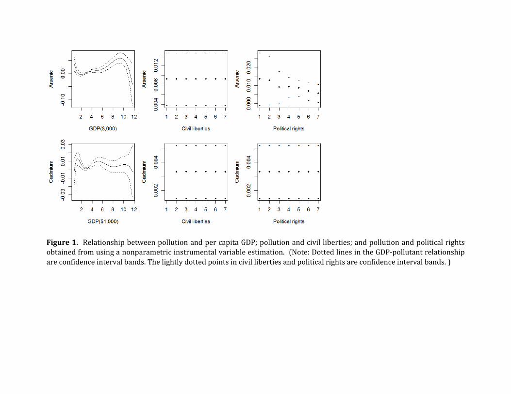
In Figure 1, we present the graphical results of the estimated relationships between water

quality and per capita GDP, political rights and civil liberties resulting from our

nonparametric instrumental variable estimation. The left column of the figure represents

the relationship between per capita GDP and pollution, the middle column represents the

relationship between political liberties and pollutant concentration and the last column

represents the relationship between pollutant concentration and civil liberties. We

describe the results for each pollutant below.

Nickel

We find a cubic relationship or N-shaped curve between nickel concentration and per

capita GDP. We do not find political rights or civil liberties impacting the nickel

concentration.

Mercury

Per capita GDP and mercury concentration seem to have a cubic relationship. However

we do not see any relationship between political rights and GDP or civil liberties and per

capita GDP.

Arsenic

Per capita GDP and arsenic pollution seem to have a cubic relationship. The lower humps

of the curve reaches first before getting to the upper hump. Arsenic pollution also

declines if there are no political rights. Civil liberties do not have any impact on the

arsenic pollution.

Cadmium

Cadmium concentration seems to have declined with increase in per capita GDP especially

after per capita GDP hits $6,000 level. However, we do not find any definitive

relationships between cadmium concentration and per capita GDP level.

Lead

We found that an inverted U-shaped relationship exists between per capita GDP and lead

concentration. There is no distinct pattern on the relationship between civil liberties and

lead pollution or political rights and lead pollution although it looks like the highest

amount of when political rights has the value equal to 5.

Fecal coliform

For fecal coliform we found almost a cubic relationship between pollution and income.

The lower turning points occurred around $4000 whereas the upper turning point is

around $10,000. Variations in political rights or civil liberties do not seem to have any

impact on the fecal coliform concentration in water bodies.

Total coliform

The relationship between total coliform and per capita GDP seem to follow almost a

polynomial of 4th degree type of relationship. The pollution level seems to reduce

substantially after the income level reaches the $11,000 level. When the level of political

rights is lower (and the political rights index is higher), total coliform concentration is

lower.

Dissolved oxygen

At lower levels of GDP, the relationship between GDP and dissolved oxygen looks flat but

once the GDP level is $8000 or higher the dissolved oxygen level starts declining. We do

see a clear quadratic relationship between political rights and GDP. There is no unique

shape observed between civil liberties and dissolved oxygen concentration.

Chemical oxygen demand

The relationship between GDP and chemical oxygen demand concentration looks like an

N-shape. We also see that higher civil liberties are associated with higher levels of

chemical oxygen demand and lower civil liberties are associated with lower levels of

chemical oxygen demand. The relationship with political rights is flat.

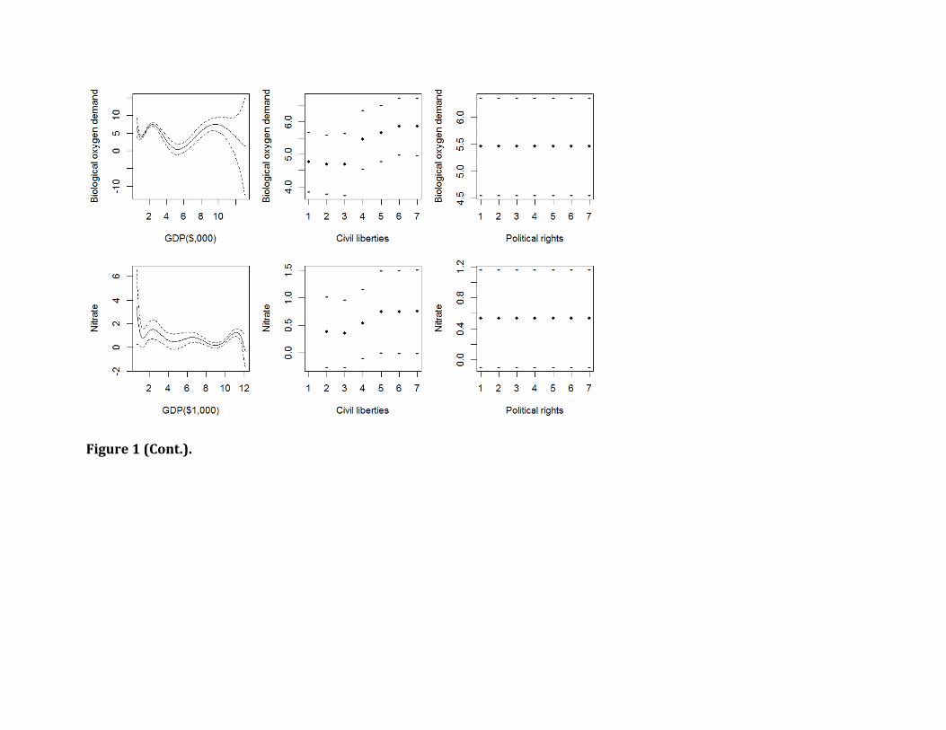
Biological oxygen demand

The biological oxygen demand curve shows 5th degree of polynomial relationship with per

capita GDP. We see a clear relationship between civil liberties and biological oxygen

demand with higher civil liberties associated with low biological oxygen demand levels

and lower civil liberties associated with higher levels of pollution. We do not find political

rights affecting the level of biological oxygen demand.

Nitrate

We did not see any distinct shape on the relationship between nitrate pollution and per

capita GDP. Higher civil liberties contribute to less amount of nitrate pollution but

political rights have no impact on the nitrate pollution. Many studies (Paudel et al. 2005

and 2009) have shown an existence of EKC curve for nitrate pollution. For the global level

water pollutants, others have shown the quadratic relationship between income and

pollution.

Conclusion

This study contributes to a better understanding of the relationships between water

pollution and per capita GDP, civil liberties, and political rights at the global level. We use

recent advances in econometric techniques to address the inclusion of continuous and

discrete variables in nonparametric instrumental variable regression models.

According to our results, we find an inverted U-shape relationship for one pollutant

(lead), and a cubic relationship for three pollutants (nickel, arsenic and fecal coliform). In

contrast, according to the results of Lin and Liscow (2013), whose model uses

instrumental variables but, unlike the model in this paper, is neither nonparametric nor

accounts for the discrete nature of the political variables, evidence for an inverted-U

relationship between income and environmental degradation were found for at least two

out of the four IV specifications for seven out of eleven water pollutants (biological oxygen

demand, chemical oxygen demand, arsenic, cadmium, lead, nickel, and fecal coliform), and

for each of these seven pollutants there is both a peak and a trough. By using a

nonparametric model that accounts for the discrete nature of the political variables, we

find that fewer pollutants exhibit an environmental Kuznets curve than were previously

found in Lin and Liscow (2013).

In terms of the political variables, we found that the arsenic and total coliform

levels decline as the level of political rights declines (and as the political rights index

increases), but lead and dissolved oxygen have an inverted U-shaped curve with political

rights. For lead and dissolved oxygen, results suggest that as countries progress towards

political rights, water pollution increases at first but then decreases after certain levels of

political rights have been attained. Our results indicate that higher biological oxygen

demand and nitrate pollution levels are associated with lower levels of civil liberties

(higher civil liberties index) but that lower chemical oxygen demand levels are associated

with lower levels of civil liberties (higher civil liberties index). Thus, factors affecting

political rights such as the fairness of the electoral process, the degree of political

pluralism and participation, and the presence of a non-corrupt and transparent

government are beneficial for water quality to some extent.

By estimating a nonparametric relationship between political variables and

pollution and by accounting for the categorical nature of the political variables, we are

able to detect a nonlinear relationship between political variables and pollution, which for

some pollutants is an inverted U-shaped curve. In contrast, Lin and Liscow (2013), whose

model uses instrumental variables but, unlike the model in this paper, is neither

nonparametric nor accounts for the discrete nature of the political variables, are unable to

tease out the nonlinear nature of some of the relationships; they instead find that the

effect of political variables on pollution can be either positive or negative depending on

pollutant and political variable.

The relationships between environmental degradation, income and political

institutions found in this study suggest that there are nonlinear relationships between

water pollution and income and between water pollution and political institutions, and

that those in the field and in academia should be open to relationships between these key

components of sustainable development.

References

Azomahou, T., F. Laisney, and P. Nguyen Van. 2006. "Economic Development and Co2 Emissions: A Nonparametric Panel Approach." Journal of Public Economics 90(6-7):1347-1363.

Barbier, E.B. 2004. "Explaining Agricultural Land Expansion and Deforestation in Developing Countries." American Journal of Agricultural Economics 86(5):1347-1353.

Barrett, S., and K. Graddy. 2000. "Freedom, Growth, and the Environment." Environment and Development Economics 5(4):433-456.

Benter, W. (1994) Computer Based Horse Race Handicapping and Wagering Systems: A Report, ed. D.B. Hausch,V.S.Y. Lo, and W.T. Ziemba, San Diego; London and Toronto: Harcourt Brace, Academic Press, pp. 183-198.

Bertinelli, L., and E. Strobl. 2005. "The Environmental Kuznets Curve Semi-Parametrically Revisited." Economics Letters 88(3):350-357.

Brock, W.A., and M.S. Taylor. 2010. "The Green Solow Model [Electronic Resource]." Journal of economic growth 15(2):127-153.

Bruvoll, A., and H. Medin. 2003. "Factors Behind the Environmental Kuznets Curve: A Decomposition of the Changes in Air Pollution." Environmental and Resource Economics 24(1):27-48.

Carson, R.T. 2010. "The Environmental Kuznets Curve: Seeking Empirical Regularity and Theoretical Structure." Review of Environmental Economics and Policy 4(1):3-23.

Copeland, B.R., and M.S. Taylor. 2004. "Trade, Growth, and the Environment." Journal of Economic Literature 42(1):7-71.

Criado, C.O. 2008. "Temporal and Spatial Homogeneity in Air Pollutants Panel Ekc Estimations." Environmental & Resource Economics 40(2):265.

Culas, R.J. 2007. "Deforestation and the Environmental Kuznets Curve: An Institutional Perspective." Ecological Economics 61(2-3):429-437.

Darolles, S., Y. Fan, J.P. Florens, and E. Renault. 2011. "Nonparametric Instrumental Regression." Econometrica 79(5):1541-1565.

Dasgupta, P., and K.-G. Mäler (1995) Poverty, Institutions, and the Environmental Resourcebase, ed. J. Behrman, and T.N. Srinivaan, vol. 3A. Amsterdam.

Dasgupta, S., B. Laplante, W. Hua, and D. Wheeler. 2002. "Confronting the Environmental Kuznets Curve." Journal of Economic Perspectives 16(1):147-168.

Deacon, R.T., and C.S. Norman. 2006. "Does the Environmental Kuznets Curve Describe How Individual Countries Behave?" Land Economics 82(2):291-315.

Farzin, Y.H., and C.A. Bond. 2006. "Democracy and Environmental Quality." Journal of Development Economics 81(1):213-235.

Gawande, K., R.P. Berrens, and A.K. Bohara. 2001. "A Consumption-Based Theory of the Environmental Kuznets Curve." Ecological Economics 37(1):101-112.

Grossman, G., and A. Krueger. 1995. "Economic Growth and the Environment." Quarterly Journal of Economics 110(2):353-377.

Harbaugh, W.T., A. Levinson, and D.M. Wilson. 2002. "Reexamining the Empirical Evidence for an Environmental Kuznets Curve." Review of Economics and Statistics 84(3):541-551.

Heerink, N., A. Mulatu, and E. Bulte. 2001. "Income Inequality and the Environment: Aggregation Bias in Environmental Kuznets Curves." Ecological Economics 38(3):359-367.

Horowitz, J.L. 2011. "Applied Nonparametric Instrumental Variables Estimation." Econometrica 79(2):347-394.

House, F. 2010. "Freedom in the World 2003: Survey Methodology", http://www.freedomhouse.org/research/freeworld/2003/methodology.htm. (accessed Dec 10, 2010)

Israel, D., and A. Levinson. 2004. "Willingness to Pay for Environmental Quality: Testable Empirical Implications of the Growth and Environment Literature." Contributions in Economic Analysis & Policy 3(1):Article 2.

Jha, R., and K.V.B. Murthy. 2003. "An Inverse Global Environmental Kuznets Curve." Journal of Comparative Economics 31(2):352-368.

Kuznets, S. 1955. "Economic Growth and Income Equality." American Economic Review 45(1):1-28.

LeBude, A.V., S.A. White, A.F. Fulcher, S. Frank, W.E. Klingeman Iii, J.-H. Chong, M.R. Chappell, A. Windham, K. Braman, F. Hale, W. Dunwell, J. Williams-Woodward, K. Ivors, C. Adkins, and J. Neal. 2012. "Assessing the Integrated Pest Management Practices of Southeastern Us Ornamental Nursery Operations." Pest Management Science 68(9):1278-1288.

Lin, C.-Y.C., and Z.D. Liscow. 2013. "Endogeneity in the Environmental Kuznets Curve: An Instrumental Variables Approach." American Journal of Agricultural Economics 95(2):268-274.

List, J.A., and C.A. Gallet. 1999. "The Environmental Kuznets Curve: Does One Size Fit All?" Ecological Economics 31(3):409-423.

Lomborg, B., and C. Pope 2003. "The Global Environment: Improving or Deteriorating?' John F. Kennedy, Jr. Forum at the Harvard Kennedy School of Government", http://www.iop.

harvard.edu/programs/forum/transcripts/environment/03.13.03.pdf (accessed 12 Aug 2010)

Luzzati, T., and M. Orsini. 2009. "Investigating the Energy-Environmental Kuznets Curve." Energy 34(3):291-300.

Ma, S., and J.S. Racine. 2011. "Additive Regression Splines with Irrelevant Categorical and Continuous Regressors." Statistica Sinica.

Ma, S., J.S. Racine, and L. Yang. 2011. "Spline Regression in the Presence of Categorical Predictors." Working paper, McMaster University and Michigan State University.

Merlevede, B., T. Verbeke, and M.D. Clercq. 2006. "The Ekc for So2: Does Firm Size Matter? ." Ecological Economics 59(4):451-461.

Millimet, D.L., J.A. List, and T. Stengos. 2003. "The Environmental Kuznets Curve: Real Progress or Misspecified Models?" Review of Economics & Statistics 85(4):1038-1047.

Nguyen Van, P., and T. Azomahou. 2007. "Nonlinearities and Heterogeneity in Environmental Quality: An Empirical Analysis of Deforestation." Journal of Development Economics 84(1):291-309.

Nie, Z., and J.S. Racine. 2012. "The Crs Package: Nonparametric Regression Splines for Continous and Categorical Predictors." The R Jouranl 4:48-56.

Paudel, K., B.N. Poudel, D. Bhandari, and T. Johnson. 2011. "Examining the Role of Social Capital in Environmental Kuznets Curve Estimation. ." Global Journal of Environmental Science and Technology:1-11.

Paudel, K.P., and M.J. Schafer. 2009. "The Environmental Kuznets Curve under a New Framework: The Role of Social Capital in Water Pollution." Environmental and Resource Economics 42(2):265-278.

Paudel, K.P., H. Zapata, and D. Susanto. 2005. "An Empirical Test of Environmental Kuznets Curve for Water Pollution." Environmental & Resource Economics 31(3):325-348.

Phu, N.V. 2003. "A Semiparametric Analysis of Determinants of a Protected Area." APPLIED ECONOMICS LETTERS 10(10):661-665.

Plassmann, F., and N. Khanna. 2006. "Household Income and Pollution: Implications for the Debate About the Environmental Kuznets Curve Hypothesis." Journal of Environment and Development 15(1):22-41.

Poudel, B.N., K.P. Paudel, and K. Bhattarai. 2009. "Searching for an Environmental Kuznets Curve in Carbon Dioxide Pollutant in Latin American Countries." Journal of Agricultural and Applied Economics 41(1):13-27.

Racine, J., and Q. Li. 2004. "Nonparametric Estimation of Regression Functions with Both Categorical and Continuous Data." Journal of Econometrics 119(1):99-130.

Rodriguez-Meza, J., D. Southgate, and C. Gonzalez-Vega. 2004. "Rural Poverty, Household Responses to Shocks, and Agricultural Land Use: Panel Results for El Salvador." Environment and Development Economics 9(2):225-239.

Roy, N., and G. Cornelis van Kooten. 2004. "Another Look at the Income Elasticity of Non-Point Source Air Pollutants: A Semiparametric Approach." Economics Letters 85(1):17-22.

Rupasingha, A., S.J. Goetz, D.L. Debertin, and A. Pagoulatos. 2004. "The Environmental Kuznets Curve for Us Counties: A Spatial Econometric Analysis with Extensions." Papers in Regional Science 83(2):407-424.

Schmalensee, R., T.M. Stoker, and R.A. Judson. 1998. "World Carbon Dioxide Emissions: 1950–2050." Review of Economics & Statistics 80(1):15-27.

Stern, D.I. (2008) The Rise and Fall of the Environmental Kuznets Curve, ed. J. Martinez-Alier, and I. Ropke, Elgar Reference Collection. Cheltenham, U.K. and Northampton, Mass.: Elgar, pp. 519-539.

Torras, M., and J.K. Boyce. 1998. "Income, Inequality, and Pollution: A Reassessment of the Environmental Kuznets Curve." Ecological Economics 25(2):147-160.

Zapata, H.O., and K.P. Paudel (2009) Functional Form of the Environmental Kuznets Curve, ed. T.B. Fomby, and R.C.l. Hill, vol. 25, Emerald Group Publishing Limited, pp. 471-493.

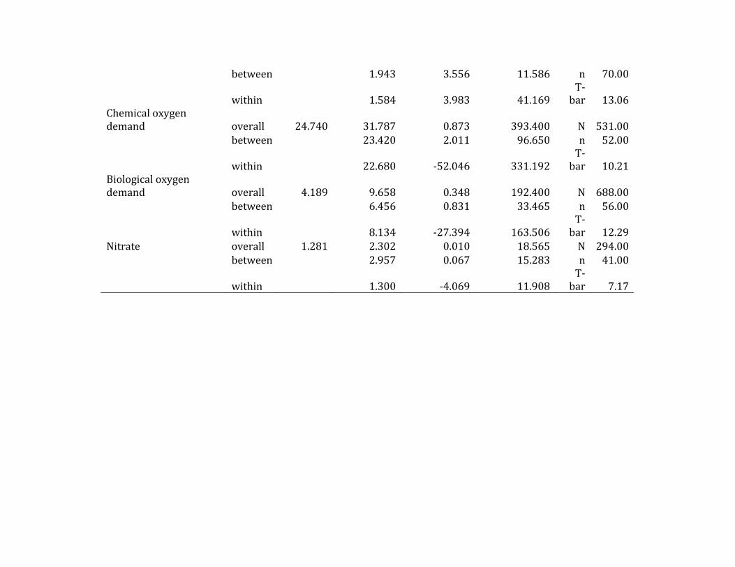
Table 1: Summary Statistics

Variable Name. M. type Mean SD Min Max Observation

Nickel overall 0.014 0.030 0.000 0.326 N 246.00 between 0.015 0.000 0.067 n 30.00

within 0.024 -0.041 0.325 T-

bar 8.20 Mercury overall 0.336 0.713 0.000 7.900 N 447.00 between 0.459 0.000 2.468 n 44.00

within 0.617 -2.133 6.937 T-

bar 10.16 Arsenic overall 0.017 0.068 0.000 0.785 N 309.00 between 0.084 0.000 0.518 n 38.00

within 0.051 -0.250 0.516 T-

bar 8.13 Cadmium overall 0.023 0.097 0.000 1.000 N 475.00 between 0.061 0.000 0.257 n 45.00

within 0.081 -0.222 0.857 T-

bar 10.56 Lead overall 0.030 0.106 0.000 1.067 N 500.00 between 0.127 0.000 0.500 n 50.00

within 0.079 -0.440 0.860 T-

bar 10.00 Fecal coliform overall 47982.37 229659.500 0.000 3681414.000 N 467.00 between 96137.040 0.000 515869.100 n 42.00

within 201667.600 -411961.200 3383963.000 T-

bar 11.12

Total coliform overall 134726.9 660444.300 0.000 10400000.000 N 431.00 between 421087.000 0.000 2593846.000 n 47.00

within 541430.600 -

2456222.000 7985642.000 T-

bar 9.17 Dissolved oxygen overall 8.389 2.497 0.000 42.500 N 914.00

between 1.943 3.556 11.586 n 70.00

within 1.584 3.983 41.169 T-

bar 13.06 Chemical oxygen demand overall 24.740 31.787 0.873 393.400 N 531.00 between 23.420 2.011 96.650 n 52.00

within 22.680 -52.046 331.192 T-

bar 10.21 Biological oxygen demand overall 4.189 9.658 0.348 192.400 N 688.00

between

6.456 0.831 33.465 n 56.00

within

8.134 -27.394 163.506

T-bar 12.29

Nitrate overall 1.281 2.302 0.010 18.565 N 294.00

between

2.957 0.067 15.283 n 41.00

within 1.300 -4.069 11.908 T-

bar 7.17

Table 1. Contd.

Variable Name. M. type Mean SD Min Max Observation

Political Rights overall 3.660 2.228 1.000 7.000 N 6017.00

between

2.006 1.000 7.000 n 203.00

within

1.006 -0.109 8.751 T-bar 29.64

Civil Liberties overall 3.665 1.935 1.000 7.000 N 6017.00

between

1.756 1.000 7.000 n 203.00

within

0.839 0.588 7.635 T-bar 29.64

Per Capita GDP overall 10.362 12.506 0.102 123.433 N 5447.00

between

12.265 0.482 70.805 n 182.00

within

3.600 -23.051 62.990 T-bar 29.93

Debt overall 5.184 5.942 0.000 135.376 N 3478.00

between

3.317 0.084 17.891 n 127.00

within 4.946 -11.697 128.428 T 27.39

Figure 1. Relationship between pollution and per capita GDP; pollution and civil liberties; and pollution and political rights

obtained from using a nonparametric instrumental variable estimation. (Note: Dotted lines in the GDP-pollutant relationship

are confidence interval bands. The lightly dotted points in civil liberties and political rights are confidence interval bands. )

Figure 1 (Cont.)

Figure 1 (Cont.).