hal-00257073, version 1 - 19 Feb 2008 Equilibrium and out of equilibrium phase transitions in systems with long range interactions and in 2D flows Freddy Bouchet ∗ , Julien Barré † and Antoine Venaille ∗∗ ∗ Institut Non Lineaire de Nice, INLN, UMR 6618, CNRS, UNSA, 1361 route des lucioles, 06 560 Valbonne - Sophia Antipolis, France † Université de Nice-Sophia Antipolis, Laboratoire J. A. Dieudonné, Parc Valrose, 06108 Nice Cedex 02, France ∗∗ Coriolis-LEGI, 21 avenue des Martyrs, 38000 Grenoble, France Abstract. In self-gravitating stars, two dimensional or geophysical flows and in plasmas, long range interactions imply a lack of additivity for the energy; as a consequence, the usual thermodynamic limit is not appropriate. However, by contrast with many claims, the equilibrium statistical mechan- ics of such systems is a well understood subject. In this proceeding, we explain briefly the classical approach to equilibrium and non equilibrium statistical mechanics for these systems, starting from first principles. We emphasize recent and new results, mainly a classification of equilibrium phase transitions, new unobserved equilibrium phase transition, and out of equilibrium phase transitions. We briefly discuss what we consider as challenges in this field. Keywords: Long range interactions, Inequivalence of ensembles, Kinetic theory, Out of equilib- rium phase transitions, Two dimensional turbulence, Geophysical flows. PACS: 05.20.Dd, 05.20.Gg, 05.70.Fh, 05.70.Ln 1. INTRODUCTION In a large number of physical systems, any single particle feels a potential dominated by interactions with far away particles: this is our definition of long range interactions. In a system with algebraic decay of the inter-particle potential V (r) ∼ r→∞ r α , this occurs when α is less than the dimension of the system (these interactions are sometimes called ”non-integrable”). Then the energy is not additive, as the interaction of any subpart of the system with the whole is not negligible with respect to the internal energy of this given part. Self gravitating stars, after the discovery of negative specific heat in [1], have played a very important historical role, by emphasizing the peculiarities in the statistical me- chanics of systems with long range interactions. Besides astrophysical self gravitating systems [2, 3, 4, 5, 6, 7, 8, 9, 10, 11], the main physical examples of non-additive sys- tems with long range interactions are two-dimensional or geophysical fluid dynamics [12, 13, 14, 15, 16, 17] and a large class of plasma effective models [18, 19, 20, 21]. Spin systems [22] and toy models with long range interactions [23, 24, 25] have also been widely studied. The links between these different subjects have been emphasized recently [23].
Transcript
hal-0
0257
073,
ver
sion
1 -
19
Feb
200
8
Equilibrium and out of equilibrium phasetransitions in systems with long range
interactions and in 2D flowsFreddy Bouchet∗, Julien Barré† and Antoine Venaille∗∗
∗Institut Non Lineaire de Nice, INLN, UMR 6618, CNRS, UNSA, 1361 route des lucioles, 06 560Valbonne - Sophia Antipolis, France
†Université de Nice-Sophia Antipolis, Laboratoire J. A. Dieudonné, Parc Valrose, 06108 NiceCedex 02, France
∗∗Coriolis-LEGI, 21 avenue des Martyrs, 38000 Grenoble, France
Abstract. In self-gravitating stars, two dimensional or geophysicalflows and in plasmas, long rangeinteractions imply a lack of additivity for the energy; as a consequence, the usual thermodynamiclimit is not appropriate. However, by contrast with many claims, the equilibrium statistical mechan-ics of such systems is a well understood subject. In this proceeding, we explain briefly the classicalapproach to equilibrium and non equilibrium statistical mechanics for these systems, starting fromfirst principles. We emphasize recent and new results, mainly a classification of equilibrium phasetransitions, new unobserved equilibrium phase transition, and out of equilibrium phase transitions.We briefly discuss what we consider as challenges in this field.
Keywords: Long range interactions, Inequivalence of ensembles, Kinetic theory, Out of equilib-rium phase transitions, Two dimensional turbulence, Geophysical flows.PACS: 05.20.Dd, 05.20.Gg, 05.70.Fh, 05.70.Ln
1. INTRODUCTION
In a large number of physical systems, any single particle feels a potential dominatedby interactions with far away particles: this is our definition of long range interactions.In a system with algebraic decay of the inter-particle potential V (r) ∼
r→∞rα , this occurs
whenα is less than the dimension of the system (these interactionsare sometimes called”non-integrable”). Then the energy is not additive, as the interaction of any subpart ofthe system with the whole is not negligible with respect to the internal energy of thisgiven part.
Self gravitating stars, after the discovery of negative specific heat in [1], have playeda very important historical role, by emphasizing the peculiarities in the statistical me-chanics of systems with long range interactions. Besides astrophysical self gravitatingsystems [2, 3, 4, 5, 6, 7, 8, 9, 10, 11], the main physical examples of non-additive sys-tems with long range interactions are two-dimensional or geophysical fluid dynamics[12, 13, 14, 15, 16, 17] and a large class of plasma effective models [18, 19, 20, 21].Spin systems [22] and toy models with long range interactions [23, 24, 25] have alsobeen widely studied. The links between these different subjects have been emphasizedrecently [23].
In these systems, the most prominent and interesting physical phenomenon is the selforganization of the particles, or of the velocity field. Thisleads to coherent clouds ofparticles in plasma physics, to galaxies and globular clusters in astrophysics and to largescale jets and vortices in two dimensional or geophysical flows. Given the large numberof particles or of degrees of freedom, it is tempting to adopta statistical approach inorder to describe these phenomena. The statistical description of such a self organization,both at the levels of equilibrium situations and relaxationtowards equilibrium (kinetictheories), is a classical, long studied field. One of the aim of this proceeding is to insiston the vitality of this old subject and to stress new advancesand remaining issues. Bycontrast, the out of equilibrium statistical mechanics of such phenomena is still in itsinfancy, and few studies have been devoted to it. We emphasize the importance of suchstudies for real applications, as most plasma and geophysical physical phenomena areout of equilibrium. We also describe some recent very suggestive results.
Both equilibrium and out of equilibrium phase transitions play a key role in our under-standing of physics, because they separate regions of parameter space with qualitativelydifferent behaviors. Very naturally, a large part of our studies will be devoted to phasetransitions. We will especially stress the peculiar association of phase transitions withnegative specific heat and statistical ensemble inequivalence in systems with long rangeinteractions. We also insist on recently observed out of equilibrium phase transtions, inthe context of two dimensional flows. Finally, we describe our personal guesses for whatmay be the challenges and interesting issues in the field of systems with long range inter-actions. We hope this could open new discussions, although we are conscious that suchguesses are necessarily biased by personal prejudices. We actually sincerely hope thatfuture researches will be much richer than what we describe.The article is organizedin three main sections: equilibrium, relaxation to equilibrium and kinetic theories, nonequilibrium stationary states.
Equilibrium. Long range interacting systems are known to display peculiar ther-modynamic behaviors. As additivity is often seen as a cornerstone of usual statisticalmechanics and thermodynamics, it is sometimes written in textbooks or articles that“statistical mechanics or thermodynamics do not apply to systems with long range inter-actions”. In this paper, we argue on the contrary that usual tools and ideas of statisticalmechanics do apply to such systems, both at equilibrium and out of equilibrium. How-ever, reviewing a variety of recent works, we will show that acareful application ofthese tools reveals truly unusual and fascinating behaviors, absent from the world ofshort range interacting systems.
After a brief introduction on the unusual negative specific heat and other peculiarthermodynamical phenomena, we discuss the usual assumptions of equilibrium statis-tical mechanics and their interpretation in systems with long range interactions. Basedon the assumption of equal probability of any configuration with a given energy, wethen explain why the Boltzmann-Gibbs entropy actually measures the probability toobserve a given distribution function. This relies on our ability to prove large deviationsresults for such systems. The result of this analysis is thatmicrocanonical and canonicalensembles of systems with long range interactions are described by two dual variationalproblems. We explain why such variational problems lead to possible generic ensembleinequivalence, and to a richer zoology of phase transitionsthan in usual systems. A
natural question then arises: do we know all possible behaviors stemming from longrange interactions, and, if not, what are the possible phenomenologies? We answerthis question by discussing aclassificationof all microcanonical and canonical phasetransitions, in long range interacting systems, with emphasis on situations of ensembleinequivalence [26]. Very interestingly many possible phase transitions and situations ofensemble inequivalence have not been observed yet. We then describe, for two dimen-sional flows, the first observation of appearance of ensembleinequivalence associatedto bicritical and azeotropy phase transitions.
Kinetic theories and relaxation toward equilibrium.Because systems with longrange interactions relax very slowly towards equilibrium,or because they can be forcedby external field, the study of out of equilibrium situationsis physically essential. Duringthe past century, there have been many attempts to find a general formalism for out ofequilibrium statistical mechanics, which would give the equivalent of the Gibbs picturefor out of equilibrium states. Unfortunately, as recognized by most of the statisticalmechanics community, until now any such attempt failed. This is mainly due to the factthat our knowledge of out of equilibrium situations can not be parameterized by a smallnumber of macroscopic quantities, playing the same role as dynamical invariants for theequilibrium theory. Then out of equilibrium statistical mechanics must be addressed bya case by case careful examination of dynamics, using some appropriate probabilisticdescription.
For relaxation to equilibrium of Hamiltonian systems with long range interactions,standard tools have been developed, mainly kinetic theory.In the introductory para-graph, we briefly explain the basic ideas of kinetic theories. In the following, we firststress the role of a Vlasov description for small time, and then the role of Lenard-Balescuequation (also called collisional Boltzmann equation in the context of self-gravitatingsystems) for larger time. We also briefly review the recent application of Lynden-Bellequilibrium statistical mechanics for the Vlasov equationto simple one dimensionalmodels. We also discuss new recent results for the kinetic theory of such systems.The first is the generic existence, for the one particle stochastic process, of anomalousdiffusion and of long relaxation times. We guess that the implications of such a resultfor the validity of the kinetic approach has not been well appreciated up to now. Thesecond class of results deals with the time of validity for the Vlasov approximationand with the typical time needed to observe relaxation towards equilibrium. One of themost striking result is that the Lenard Balescu operator vanishes identically for onedimensional systems. This explains the existence of anomalous scaling laws for therelaxation towards equilibrium in models like the HMF model.
Non equilibrium stationary states (NESS).Another class of out of equilibrium prob-lems is the study of systems with long range interactions subjected to small non-Hamiltonian forces and to weak dissipation. Such a framework is actually the most rele-vant one for many physical applications. We will emphasize its interest for geophysicalflows, like for instance simplified models of ocean currents.
FIGURE 1. Caloric curve (temperatureT = β−1 as a function of the energyU) for the SGR model,for ε = 10−2. The energies corresponding to the dashed vertical lines are referred to, from left to right,asUlow, Utop, Uc, andUhigh. The decreasing temperature betweenUtop andUc characterizes a range ofnegative specific heat and thus of ensemble inequivalence. At Uc, there is a microcanonical second orderphase transition associated with the canonical first order phase transition (please see the text for a detailedexplanation). Such a behavior is linked to the existence of tricritical points in both statistical ensembles(see figure 2). A classification of all possible routes to ensemble inequivalence is briefly described insection 2.4 or in [26].
The average balance between forcing and dissipation usually leads to statisticallystationary states, the properties of which may be studied experimentally, numericallyand theoretically. As there is no detailed balance, the system is maintained out ofequilibrium. The fluxes of the Hamiltonian conserved quantities then become essentialphysical variables.
We show in this last section, that this leads, in the context of two dimensional flows,to very interesting out of equilibrium phase transitions. We believe that the study of thestatistical mechanics of such non equilibrium stationary states and phase transitions, inother systems with long range interactions, is one of the main challenges in this field.
2. EQUILIBRIUM STATISTICAL MECHANICS OF SYSTEMSWITH LONG RANGE INTERACTIONS
2.1. Peculiarities of thermodynamics of systems with long rangeinteractions
For systems with long range interactions, the most intriguing thermodynamical prop-erty is the generic occurrence of statistical ensemble inequivalence and negative specificheat. Such possibilities have first been recognized and studied in the context of selfgravitating systems [1, 27, 11]. Afterwards, ensemble inequivalence and negative spe-cific heat have been observed or predicted in a number of different physical systems:two dimensional turbulence [12, 28, 29], plasma physics [28, 19], spin systems or toymodels [22, 25], or self gravitating systems in situations different from the simple initialcase [7, 5, 3, 4, 6, 30, 9]. A detailed description of each of these cases is provided in[26].
-1.5
-1
-0.5
0
0.5
1
1.5
10-6 10-5 0.0001 0.001 0.01 0.1 1
U
Softening parameter
-350
-300
-250
-200
-150
-100
-50
0
50
10-6 10-5 0.0001 0.001 0.01 0.1 1
U
Softening parameter
FIGURE 2. Phase diagrams for the SGR model. Left: for each value ofε, the critical energies wherea microcanonical phase transition occurs are represented by black points or circles. When the softeningparameter is varied, at the tricritical pointε = εµ
T , first order phase transitions (black points) change tosecond order phase transitions (circles). Right: the bottom dashed line and black line represent respectivelyUlow (see fig. 1) andUhigh. The differenceUhigh−Ulow is the energy jump associated to a first order phasetransition in the canonical ensemble. This jump decreases to zero at canonical tricritical pointεc
T where thecanonical first order phase transition changes to a canonical second order phase transition. The tricriticalpoints have different energies andε values in both ensembles.
To motivate the following development, let us give an example where ensemble in-equivalence appears in an unusual way. We discuss the equilibrium properties of theSelf Gravitating Ring (SGR) model, a toy model for self gravitating systems. Whereaswe mainly present here its equilibrium properties, we stress that this system is very in-teresting also from a dynamical point of view, as it shows a number of out of equilibriumquasi-stationary states [31, 32].
The Hamiltonian of the SGR model is:H = 12 ∑N
i=1 p2i − 1
2 ∑Ni, j=1
1√2
1√1−cos(θi−θ j )+ε
.
Particles are constrained on a ring (0≤ θi ≤ 2π). The anglesθi are conjugate to themomentapi . ε is a small scale softening of the gravitational interaction. We study thephase transitions of this system and how they evolve whenε is varied. Please see [30]for a detailed discussion.
Figure 1 shows the caloric curveT(U) for ε = 10−2, whereT is the temperatureandU is the energy. ForUtop < U < Uc the temperature is decreasing. The specificheatC = dU/dT is thus negative in this area, showing that statistical ensembles arenot equivalent (in the canonical ensemble, the specific heatis always positive). Thehorizontal dashed line is the Maxwell construction, which links microcanonical andcanonical ensembles. From it one sees that in the canonical ensemble, whenβ is varied,there is a first order phase transition characterized by an energy jump between the valuesUlow andUhigh. This is a common feature in case of ensemble inequivalence.
What is less common is the concomitant existence of a second order phase transitionin the microcanonical ensemble, at the energyUc. At this point, the temperatureT iscontinuous, whereas its derivative is discontinuous as it is clear from the curve. In figure2, we show that this type of ensemble inequivalence, with thecoexistence of a firstorder canonical first order phase transition and of a microcanonical second order phasetransition, is linked to the existence of a tricritical point in both ensembles.
The SGR model displays one possible route to ensemble inequivalence, out of sev-eral others. However, there are some constraints on the possible phenomenologies. Forinstance, at a second order phase transition, the negative specific heat jump must be pos-itive. By contrast, the temperature jumps at a discontinuity associated with a first ordermicrocanonical phase transition must be negative (this means that when energy is in-creased the system has a negative temperature jump). Summarizing all these constraintsyields aclassification[26] of all possible ensemble inequivalences and their links withphase transitions. To prepare the discussion of this classification, we recall now the mainhypothesis and definitions of statistical equilibrium, in the context of systems with longrange interactions.
2.1.1. Additivity extensivity and thermodynamic limit
When studying statistical mechanics of non additive systems, the first problem onehas to deal with is the inadequacy of the thermodynamic limit(N → ∞, V → ∞ -V isthe volume-, withN/V kept constant). Indeed, what is physically important in order tounderstand the behavior of large systems, is not really to study the largeN limit, butrather to obtain properties that do not depend much onN for largeN (the equivalentof intensive variables). For short range interacting systems, this is achieved through thethermodynamic limit; for non additive systems, the scalinglimit to be considered isdifferent and depends on the problem. Let us considerN particles which dynamics isdescribed by the Hamiltonian
HN =12
N
∑i=1
p2i +
c2
N
∑i, j=1
V(xi −x j) , (1)
wherec is a coupling constant. The thermodynamic limit in this caseamounts to sendN and the volume to infinity, keeping density andc constant. IfV(x) decreases fastenough so that interactions for a particle come mainly from the first neighbors, thenincreasingN at constant density has almost no effect on the bulk, and physical propertiesare almost independent ofN: the thermodynamic limit is appropriate. This is wrong ofcourse if the potential for a particle is dominated by the influence of far away particles.The appropriate scaling in this case may be as follows: fixed volume,c ∝ 1/N2, andN → ∞ (others equivalent combinations are possible, as the one given below for selfgravitating particles).
The best known example of such a special scaling concerns self gravitating stars, forwhich the rationM/R is usually kept constant, whereM is the total mass andR is thesystem’s radius (thermodynamic limit would beM/R3 constant). Another toy exampleis given and studied for instance in [33]. This type of scaling is also the relevant one forpoint vortices in two dimensional and geophysical turbulence, where the total volumeand total vorticity have to be kept fixed, but divided in smaller and smaller units. Letus note for completeness that in some cases, the thermodynamic limit is appropriate inpresence of long range interactions, for instance when somescreening is involved [34];we shall exclude these cases in the following.
According to the above discussion, let us rewrite Eq. 1 usingthe convenient scalingc = ±1/N:
HN =12
N
∑i=1
p2i ±
12N
N
∑i, j=1
V(xi −x j) (2)
This classical scaling of the coupling parameter is called the Kac’s prescription ([35])or sometimes the mean field scaling (see for instance [36]). Within this scaling, takingthe limit N → ∞ with all other parameters fixed (fixed volume for instance), the sumover i and j is clearly of orderN2, and the energy per particleHN/N is intensive. Thisscaling is also the relevant one in order to obtain the collisionless Boltzmann equation,for the dynamics, in the largeN limit. We will use Eq. 2 in the following.
2.1.2. The microcanonical and canonical ensembles
We suppose that the energyE of our system is known, and consider the microcanon-ical ensemble. In this statistical ensemble all phase spaceconfigurations with energyEhave the same probability; the associated microcanonical measure is then
µN =1
ΩN (E)
N
∏i=1
dxidpiδ (HN (xi , pi)−E) ,
where ΩN (E) is the volume of the energy shell in the phase spaceΩN (E) ≡∫∏dxidpiδ (HN (xi , pi)−E). We consider here the energy as the only parameter,
however generalization of the following discussion to other quantities conserved by thedynamics is straightforward.
The only hypothesis of equilibrium statistical mechanics is that averages with respectto µN will correctly describe the macroscopic behavior of our system. This hypothesisis usually verified after a sufficiently long time, when the systems has “relaxed” toequilibrium.
The Boltzmann entropy per particle is defined as
SN (E) ≡ 1N
logΩN (E)
In the following, we will justify that in the long range thermodynamic limit, the entropyper particleSN (E) has a limit:
SN (E) →N→∞
S(E)
The canonical ensemble is defined similarly, using the canonical measure
2.2.1. Justification of the Boltzmann-Gibbs entropy
Let us consider the particle distribution onµ−spacef (x, p) ( f (x, p)dxdpis the prob-ability to observe a particle with positionx and momentump). f defines a macrostateas many microscopic states correspond to a givenf . As explained in the previous para-graph, the hypothesis of usual statistical mechanics is that all microscopic states with agiven energyE are equiprobable. Given this uniformity in phase space, we address thequestion: what is the number of microscopic states having the distributionf ?
It is a classical combinatorial result to show that the logarithm of number of micro-scopic states corresponding to a distributionf is given by
s[ f ] = −∫
dxdp flog f
wheres is sometimes called the Boltzmann-Gibbs entropy. It is the Boltzmann entropyassociated to the macrostatef , in the sense that it counts the number of microstatescorresponding tof . We stress thatno other functional has this probabilistic meaning,and that this property is independent of the Hamiltonian.
Thanks to the long range nature of the interaction, for most configurations, the energyper particle can be expressed in term of the distribution function f , using
h( f ) ∼N→∞
∫p2
2f (x, p)dx dp +
∫dx1dp1dx2dp2 f (x1,p1) f (x2,p2)V(x1−x2). (3)
This mean field approximation for the energy allows to conclude that the equilibriumentropy is given by
SN (E) = log(ΩN (E)) ∼N→∞
NS(E) with S(E) = supfs( f ) | h( f ) = E (4)
In the limit of a large number of particles, the mean field approximation Eq. (3) and itsconsequence the variational problem (4) have been justifiedrigorously for many systemswith long range interactions. The first result assumes a smooth potentialV and hasbeen proved by [36], see also the works by Hertel and Thirringon the self gravitatingfermions [27].
2.2.2. Large deviations
We explained why the Boltzmann-Gibbs entropy is the correctone to describe theprobability of a givenf . Large deviations provide a useful tool to obtain similar resultsin a wider context. We refer to the very interesting contributions of Ellis and coworkers([37, 29, 38, 39, 40]). We also refer to [41] for a simple detailed explanation of manylarge deviations results in the context of long range interacting systems.
In a first step one describes the system at hand by a macroscopic variable; thismay be a coarse-grained density profilef , a density of charges in plasma physics, a
magnetization profile for a magnetic model. In the following, we will generically callthis macroscopic variablem; it may be a scalar, a finite or infinite dimensional variable.
One then associates a probability to each macrostatem. Large deviation theorycomes into play to estimateΩ(m), the number of microstates corresponding to themacrostatem:
log(ΩN (m)) ∼N→∞
Ns(m) .
This defines the entropys(m).In a second step, one has to express the constraints (energy or other dynamical
invariants) as functions of the macroscopic variablem. In general, it is not possible toexpress exactlyH; however, for long range interacting systems, one can definea suitableapproximating mean field functionalh(m), as in Eq. (3).
Having now at hand the entropy and energy functionals, one can compute the micro-canonical density of statesΩ(E) ([37]): the microcanonical solution is simply given bythe variational problem
log(ΩN (E)) ∼N→∞
NS(E) with S(E) = supm
s(m) | h(m) = E (5)
In the canonical ensemble, similar considerations lead to the conclusion that the freeenergy and the canonical equilibrium are given by the variational problem
log(ZN (β )) ∼N→∞
NF(β ) with F (β ) = infm−s(m)+βh(m) (6)
We insist that this reduction of the microcanonical and canonical calculations to thevariational problems (5) and (6) is in many cases rigorouslyjustified.
2.3. Ensemble equivalence and simplification of variational problems
As discussed in the previous section, the microcanonical and canonical equilibriumstates are, most of the times, given by (5) and (6) respectively. These two variationalproblems are dual ones: the canonical one is obtained from the microcanonical oneby relaxing a constraint. In the following section, we discuss the mathematical linksbetween two such dual variational problems. We then apply this to characterize ensembleequivalence, and we use it to prove relations between classes of variational problems.
2.3.1. Relations between constrained and relaxed variational problems
It is possible to state some general results about the variational problems (5) and (6),independently of the precise form of the functionss andh:
1. a minimizermc of (6) is a minimizer of (5), with constraintE = h(mc).2. a minimizermµ of (5) is a critical point of (6) for someβ , but it is not always a
minimizer: it is a minimizer of (6) if and only ifScoincides with its concave hull atpointE = h(mµ). Otherwise, it may be a local minimum, or a saddle point of (6).
Such results are extremely classical. More detailed results in this context may befound in [37]. We also refer to [42] for a concise discussion and proof. The previouspoints immediately translate into the language of statistical mechanics, and provide afull characterization of ensemble inequivalence:
• A canonical equilibrium is always a microcanonical equilibrium for some energyE.• A microcanonical equilibrium at energyE is a canonical equilibrium for some
temperature 1/β if and only if S coincides with its concave hull at energyE.WheneverS coincides with its concave hull, we will say that the ensembles areequivalent; otherwise we will say they are not equivalent.
2.3.2. Simpler variational problem for statistical equilibria
In the previous paragraph, we have explained relations between solutions of a con-strained variational problem and of the associated relaxedone. Using similar resultsand further theoretical considerations, it is possible to obtain much simpler variationalproblems than the natural microcanonical ones, for the equilibria of Euler and Vlasovequations [42]. We think that these new results provide essential simplifications thatwill be useful in many studies, we thus describe them in this section. However, from aphysical point of view, these mathematical results may be viewed as technical, and weadvise the non expert reader to skip this section at first reading.
When studying statistical equilibria of systems with long range interactions, one hasto deal with variational problems with one or several constraints. In the case of thestatistical mechanics of the Euler (resp. the Vlasov equation), there is actually an infinitenumber of Casimir’s functional conservation laws, encodedin the initial distributiondof the vorticity field (resp. the particle distribution function). This is a huge practicallimitation. When faced with real phenomena, physicists canthen either give physicalarguments for a given type of distributiond (modeler approach) or ask whether thereexists some distributiond with equilibria close to the observed field (inverse problemapproach). However, in any case the complexity remains: theclass of equilibria is huge.
In the following of this paragraph, we describe recent mathematical results whichallow to relate the microcanonical equilibria to much simpler variational problems.From a physical point of view, this simplification is extremely interesting. We describethese results in the context of the equilibrium theory for the Euler equation (RobertSommeria Miller theory [15, 14] or RSM theory), but the following results may beeasily generalized to other cases like the statistical mechanics of the Vlasov equation.We refer to [42] for a more detailed discussion.
>From a mathematical point of view, one has to solve a microcanonical variationalproblem (MVP): maximizing a mixing entropyS [ρ] = −
∫D d2x
∫dσ ρ logρ, with
constraints on energyE and vorticity distributiond
S(E0,d) = supρ|N[ρ]=1
S [ρ] | E [ω ] = E0 ,D [ρ] = d (MVP).
ρ (x,σ) depends on spacex and vorticityσ variables.During recent years, authors have proposed alternative approaches, which led to prac-
tical and/or mathematical simplifications in the study of such equilibria. As a first exam-ple, Ellis, Haven and Turkington [29] proposed to treat the vorticity distribution canon-ically (in a canonical statistical ensemble). From a physical point of view, a canonicalensemble for the vorticity distribution would mean that thesystem is in equilibriumwith a bath providing a prior distribution of vorticity. As such a bath does not exist, thephysically relevant ensemble remains the one based on the dynamics: the microcanon-ical one. However, the Ellis-Haven-Turkington approach isextremely interesting as itprovides a drastic mathematical and practical simplification to the problem of comput-ing equilibrium states. A second example, largely popularized by Chavanis [43, 44], isthe maximization of generalized entropies. Both the prior distribution approach of El-lis, Haven and Turkington or its generalized thermodynamics interpretation by Chavanislead to a second variational problem: the maximization of Casimir’s functionals, withenergy constraint (CVP)
C(E0,s) = infω
Cs[ω] =
∫
Ds(ω)d2x | E [ω] = E0
(CVP)
whereCs are Casimir’s functionals, andsa convex function (Energy-Casimir functionalsare used in classical works on nonlinear stability of Euler stationary flows [45, 46],and have been used to show the nonlinear stability of some of RSM equilibrium states[14, 47]).
Another class of variational problems (SFVP), that involvethe stream function only(and not the vorticity), has been considered in relation with the RSM theory
D(G) = infψ
∫
Dd2x
[−1
2|∇ψ|2+G(ψ)
] (SFVP)
Such (SFVP) functionals have been used to prove the existence of solutions to the equa-tion describing critical points of (MVP) [47]. Interestingly, for the Quasi-geostrophicmodel, in the limit of small Rossby deformation radius, sucha SFVP functional is sim-ilar to the Van-Der-Walls Cahn Hilliard model which describes phase coexistence inusual thermodynamics [17, 48]. This physical analogy has been used to make precisepredictions in order to model Jovian vortices [17, 49]. (SFVP) functionals are muchmore regular than (CVP) functionals and thus also very interesting for mathematicalpurposes.
When we prescribe appropriate relations between the distribution functiond, thefunctionss andG, the three previous variational problems have the same critical points.This has been one of the motivations for their use in previousworks. However, aclear description of the relations between the stability ofthese critical points is stillmissing (Is a (CVP) minimizer an RSM equilibria? Or does an RSM equilibria minimize(CVP)?). This has led to fuzzy discussions in recent papers.Providing an answer isa very important theoretical issue because, as explained previously, it leads to deepmathematical simplifications and will provide useful physical analogies.
In [42] we establish the relation between these three variational problems. The result isthat any minimizer (global or local) of (SFVP) minimizes (CVP) and that any minimizer
of (CVP) is an RSM equilibria. The opposite statements are wrong in general. Forinstance (CVP) minimizers may not minimize (SFVP), but may be instead only saddles.Similarly, RSM equilibria may not minimize (CVP) but be onlysaddles, even if noexplicit example has yet been exhibited.
These results have several interesting consequences :
1. As the ensemble of (CVP) minimizers is a sub-ensemble of the ensemble of RSMequilibria, one can not claim that (CVP) are more relevant for applications thanRSM equilibria.
2. The link between (CVP) and RSM equilibria provides a further justification forstudying (CVP).
3. Based on statistical mechanics arguments, when looking at the Euler evolution ata coarse-grained level, it may be natural to expect the RSM entropy to increase.There is however no reason to expect such a property to be truefor the Casimir’sfunctional. As explained above, it may also happen that entropy extrema be (CVP)saddles.
2.4. Classification of phase transitions
Beyond the full characterization of ensemble inequivalence we have described above,there are many other qualitative features of the thermodynamics that depend only on thestructureof the variational problems (5) and (6). Indeed, although the precise form ofthe solution obviously depends on the problem at hand through the functionss(m) andh(m), it is possible toclassifyall the different phenomenologies that one may find inthe study of a particular long range interacting system. Thequestions in that respect are,increasing complexity at each step:
• what are the different possible types of generic points on anentropy curveS(E)(these correspond to different phases)?
• what are the possible singular points of a genericS(E) curve (these correspond tophase transitions)?
• what are the possible singular points on theS(E) curve, when an external parameteris varied in addition to the energy (that is how phase transitions evolve when aparameter is varied)?
We address these different levels in the following paragraphs, using results from [37, 26].These results are obtained by adapting to the dual variational problems (5) and (6)ideas that lead to the Landau classification of phase transitions. In the long range casehowever, there is no approximation involved, so the classification does not suffer fromthe problems of standard Landau theory (wrong critical exponents for instance).
E
S
E
equi inequi1
inequi2
β
FIGURE 3. The three types of generic points; on the left: entropyS(E) curve, on the right: caloricβ (E)curve. Thick, thin and dashed lines correspond respectively to the three types of points. The dotted linesshows the Maxwell construction giving the canonical solution in the inequivalence range.
E
S
E
S
A
C
B
FIGURE 4. The three types of phase transitions (Codimension 0 singularities), for a system with nosymmetry.A: canonical 1st order transition.B: canonical destabilization (a local minimum of (6) becomesa saddle point).C: microcanonical 1st order, temperature jump.
2.4.1. Generic points of an entropy curve
There are three types of generic points on the entropy curve,see Fig. 3:
• Concave points (that isCv > 0) where canonical and microcanonical ensembles areequivalent.
• Concave points where ensembles are not equivalent.• Convex points (Cv < 0), where ensembles are always inequivalent.
2.4.2. Singular points of a generic entropy curve: phase transitions
Generic points as described above define segments of entropycurves, separated bysingular points, that can be of several types. These points for systems without symmetryare classified in Fig. 4.
β(E)
S
E
S
E
S
E
S
E
S
E
S
E
S
E
S
E
S
E
E
β
E
β
E
β
E
β
E
β
E
β
E
β
E
β
E
β
S
E
S
E
S
EE
β
E
β
E
β
S
E
S
E
S
E E
β
E
β
E
β
S
E
S
E
S
E E
β
E
β
E
β
Singularities
Critical point
Max
imiz
atio
n si
ngul
ariti
esAzeotropy
invisible
Azeotropy
Canonical
Triple point invisible
S(E)
Convexitymodification Critical point
First order and cano. destab.
invisibleCon
vexi
ty
Concavification Triple point
FIGURE 5. Classification of singularities, when one external parameter is varied (codimension 1singularities). The first two columns give the singularity origin and name; the third one gives its status inthe canonical ensemble: invisible means it has no consequence on the canonical solution; the six followingplots are entropic and caloric curves showing the crossing of the singularity when the external parameter isvaried. One recovers the usual phase transitions (triple point, azeotropy, critical point) in both ensembles.What is new is the list of the possible links between the behaviors in each ensemble, and the associatedappearance of ensemble inequivalence. Please see [26] for amore detailed explanation, and singularitiesassociated with symmetry breaking.
2.4.3. Singular points on a singular entropy curve
When an external parameter is varied, the entropy curve is modified. Some specialvalues of the parameter correspond to qualitative changes for the phase transitions. Allthese possible qualitative changes are classified in [26]; Fig. 5 summarizes the results.
All types of phase transitions and ensemble inequivalencesfound in the literatureso far are reproduced in the classification. In addition, theclassification predicts thepossibility of new phenomenologies, and new routes to ensemble inequivalence, thathave not so far been observed in any specific model.
2.5. Examples of new phase transitions
In the previous section we explained the existence of many yet unobserved appearanceof ensemble inequivalence, associated to phase transitions, as described in [26]. Morerecently the new finding of two such examples have been reported [50]: bicriticalpoints (a bifurcation from a first order phase transition towards two second order phasetransitions) and second order azeotropy (the simultaneousappearance of two secondorder phase transitions at a bifurcation). We present here these new phase transitions;they are associated with equilibrium states of the two dimensional Euler equation, whenthere is a linear relation between vorticity and stream function. This was first studiedby Chavanis and Sommeria [51] in the context of the Robert-Sommeria-Miller (RSM)
statistical mechanics of 2D flows [15, 14]. They found a criterion for the existenceof a transition from a monopole to a dipole above a critical energy, for all (closed)domain geometry. In this section, we present an alternativemethod providing the samecriterion, which generalizes to a large class of models, andthus shows the universalityof the phenomenon. More interestingly this new method clarifies the nature of the phasetransitions involved in this problem and makes the link withthe existence of an ensembleinequivalence region. Those results are presented in a moregeneral context in [50],where we note the interest of these phase transitions for very simple ocean models.
Euler equation and associated variational problem.Let us consider the 2D Eulerequation in a closed domainD . It can be written as a transport equation for the vorticityω = ∆ψ: ∂tω +u.∇ω = 0. The velocity fieldu is related toω via the stream functionψ:u = ez×∇ψ, with ψ = 0 on∂D . We introduce the projectionsωi of the vorticityω on acomplete orthonormal basis of eigenfunctionsei(x,y) of the Laplacian:∆ei = λiei , wherethe λi (all negative) are in decreasing order. The stationary states of this equation areprescribed by a functional relationω = f (ψ). In the following we consider the solutionsof the variational problem:
S(E,Γ) = maxω
S [ω] | E [ω] = E & C [ω] = Γ (7)
The variational problem (7) is similar to the generic problem (5) studied above, with twoconstraints instead of one.
• S is the entropy of the vorticity fieldω; we restrict ourselves to a quadratic
functional:S [ω] = −12
⟨ω2
⟩D
= −12 ∑ω2
i .
• E is the total energy:E [ω] = 12
⟨(∇ψ)2
⟩D = −1
2 ∑i λiω2i
• C is the circulation:C [ω] = 〈ω〉D = ∑i 〈ei〉ωi where〈ei〉 =∫D ei(x,y)dxdy
To compute critical points of the variational problem (7), we introduce two Lagrangeparametersβ andγ, associated respectively with the energy and the circulation conserva-tion. Those critical points are stationary solutions for the initial transport equation withf (ψ) = βψ − γ. The solutions of the variational problem will thus providethe equilib-rium states of the Euler equation that present a linear relationship between vorticity andstream function, for a given energy and circulation.
The aim of the following paragraphs is to determine which ones among the criticalpoints are solutions of (7). It will then be possible to draw aphase diagram in the plane(Γ,E) for those equilibrium states.
Dual quadratic variational problems. The problem (7), with two constraints, will bereferred to as the microcanonical problem. As already explained earlier, it is sufficientto study the easier unconstrained ensembles, unless there is inequivalence of ensembles.The strategy is then the following. Start with the easiest problem:
J(β ,γ) = minq−S [ω] +β E [ω]+ γC [ω] (grand canonical). Check if allpossible values ofE or Γ correspond to a grand canonical solution; if yesthe problem is solved, otherwise, we turn to the more constrained problem:F(β ,Γ) = minq−S [q] +β E [q] | C [q] = Γ (canonical).
In principle we could eventually have to solve the microcanonical problem. However,in this case, we will see that the microcanonical ensemble isequivalent to the canonicalone: the whole range ofE andΓ will be covered by canonical solutions.
We notice first thatS , E are quadratic functionals and thatC is a linear functional.We will thus have to look for the minimum of a quadratic functional with a linear part.
Let us callQ the purely quadratic part andL the linear part of this functional. Then wehave three cases
1. The smallest eigenvalue ofQ is strictly positive. The minimum exists and is achieved by aunique minimizer.
2. At least one eigenvalue ofQ is strictly negative. There is no minimum.3. The smallest eigenvalue ofQ is zero (with eigenfunctione0). If Le0 = 0 (case 3a), the
minimum exists and each state of the neutral directionαe0 is a minimizer. IfLe0 6= 0,(case 3b) then no minimum exists.
The grand canonical ensemble.In that case the quadratic operatorQ associated toJ = −S +β E + γC is diagonal in the Laplacian eigenvector basis. The variationalproblem admits a unique solution if and only ifβ > λ1 (case 1. above). Ifβ = λ1(case3. above), a neutral direction exists if and only ifγ = 0. By computing the energyand circulation of all those states, we prove that there is a unique solution at eachpoint in the diagram(E,Γ), below a parabolaP (see figures 6 and 7-a). Becausethe values of energies above the parabolaP are not reached, we conclude that thereis ensemble inequivalence for parameters in this region. Wethen turn to the moreconstrained canonical problem to find solutions in this area.
The canonical ensemble.The circulation is now fixed. We first transform this prob-lem into an unconstrained variational problem. By using thecirculation constraint, weexpress one coordinate in term of the others:ω1 = (Γ−∑i ωi〈ei〉)/〈e1〉. This expres-sion is then injected in the functionalF = −S + βE . The problem is now to find aminimizerωii≥2 of this functional, without constraints. This case requires more com-putations that the previous one since the operatorQ associated to the quadratic part ofF is no more diagonal in the basisei.
We first notice that if the domain geometry admits one or more symmetries, it gener-ically exists eigenfunctions having the property〈ei〉 = 0. In the subspace spanned byall those eigenfunctions,Q is diagonal, and its smallest eigenvalue is positive as longasβ > β 0
1 , whereβ 01 is the greatestλi on this subspace. Then we look for the value of
β such that the smallest eigenvalue ofQ is zero in the subspace spanned by eigenfunc-tions with〈ei〉 6= 0. Let us callβ ∗ this value, andω∗ the corresponding eigenfunction:Q[ω∗] = 0. We find after some manipulation thatβ ∗ is the greatest zero of the func-tion f (x) = 1− x∑i≥1〈ei〉2/(x−λi). We conclude that there is a single solution to thevariational problem if and only ifβ > max
(β 0
1 , β ∗). Whenβ = max(β 0
1 , β ∗), we dis-tinguish two cases according to the sign ofβ 0
1 −β ∗ to discuss the existence of a neutraldirection:
• i) β 01 < β ∗ we then considerβ = β ∗. There is a solution (case 3a) ifΓ = 0 and no solution
(case 3b) forΓ 6= 0.• ii) β 0
1 > β ∗ we then considerβ = β 01 . There is a solution (case 3a) for all values ofΓ.
FIGURE 6. Case i) Phase diagram for a domain having no symmetry, or witha symmetry axis in thecaseβ ∗ < β 0
1 . a) Internal parameters are circulationΓ and energyE. Straight line: first order transition.ParabolaP: above this line there is no grand canonical solutions; onlycanonical and microcanonicalsolutions exist. It corresponds to an ensemble inequivalence region. b) examples of flow. c) EquilibriumentropyS as a function ofE andΓ. We see clearly a region where the concave envelop ofS(E,Γ) isnot equal toS(E,Γ), which includes the first order transition line; d)β = ∂S/∂E at fixedΓ: there isno singularity. e)γ = ∂S/∂Γ at fixed E: there is a discontinuity ofγ at Γ = 0 (first order transition).The Maxwell construction shows that the ensemble inequivalence region is associated with a first ordertransition in the ensemble where the value of the energy is fixed.
We thus obtain a criterion, namely the sign ofβ 01 − β ∗, that provides two classes of
phase diagrams. This criterion depends only on the domain geometry. If the domainadmits a symmetry axis, and is sufficiently stretched in a direction perpendicular to thisaxis, thenβ 0
1 > β ∗. For an ellipse, this is always the case. However, there are domainswith a symmetry axis for which one can find a critical aspect ratio τc that separates thetwo cases. This is for instance the case of rectangular domains. Forτ > τc , case ii) isrealized (β 0
1 > β ∗) and forτ < τc, case i) is realized (β 01 < β ∗). To conclude, we find
two classes of phase diagrams:
• i) Domain without symmetry, or with symmetry with aspect ratio τ < τc (see figure6). If Γ 6= 0, all energy values are reached in the canonical ensemble, and there is asingle solution for each point(Γ,E). If Γ = 0 (straight line on figure 6), two statescoexist for each energy valueE, andβ = β ∗.
• ii) Domain with symmetry and with an aspect ratioτ > τc (see figure 7). There is aunique canonical solution at each point of the diagram belowa parabolaP0 in theplane(E,Γ) (see the dashed line figure 7). Above this parabola,β = β 0
1 , and there is
FIGURE 7. Case ii) Phase diagram for a domain having a symmetry axis, and sufficiently stretchedin a direction perpendicular to this axis (caseβ ∗ > β 0
1 ). a),b),c),d),e): see figure (6). Dashed parabolaP0: second order transition line. Above this line,∂S/∂E = β 0
1 , and the choice of one state among twopossibilities breaks the system’s symmetry. We see that∂β/∂E is discontinuous at pointG, as well as∂γ/∂Γ at pointsB andC, which is the signature of a second order phase transition.
two canonical solutions at each point of the diagram. They differ only by the sign ofthe contribution of the Laplacian eigenvector associated to the eigenvalueβ 0
1 (it is adipole). Below the Parabola, this eigenmode has no contribution to the solution. Thechoice of one solution among the two possibilities breaks the system’s symmetrywhenP0 is crossed. At high energy, the contribution of the dipole isdominant.
In both cases we find that all circulation and energy values have been reached bycanonical solutions. We conclude that microcanonical and canonical ensembles areequivalent: all microcanonical solutions are also canonical solutions.
Description of phase transitions.The difference between the two classes of flowis the existence of either first or second order phase transitions, corresponding respec-tively to case i) and ii). The main observation is that first order and second order mi-crocanonical transitions always take place in the ensembleinequivalence area. In thatrespect, those transitions are signatures of ensemble inequivalence for this class of two-dimensional flows, which could be observed in laboratory experiments on quasi twodimensional flows.
The transition from systems of type i) to systems of type ii),when the geometryis modified, leads to one of the predicted, but yet unobservedphase transition of theclassification [26], described here in sectionClassification of Phase Transitions. On
FIGURE 8. Bicritical point (from Ref. [50]) for a rectangular domain with aspect ratioτ. Bifurcationfrom a first order transition line to two second order phase transition lines. Insets are schematic projectionsof the EntropyS [ω ] in a plane(ω0
1 ,ω∗), by taking into account the constraints. M: maximum. m:minimum. s: saddle.
figure 8, we consider a fixed energy, and present the phase diagram in the(Γ,τ) plane,whereτ is an external parameter characterizing the aspect ratio ofthe domain. In themicrocanonical ensemble, there is a bifurcation from a firstorder transition line to twosecond order transition lines at a critical valueτ = τc. Such a bifurcation is referred toas a bicritical point.
2.6. Challenges in the equilibrium statistical mechanics
It seems fair to say that the equilibrium statistical mechanics of long range interactingsystems is well understood at a fundamental level, despite the important differences withthe short range case. However, some challenges and questions remain open; we mentionhere some of them.
A first issue is the relevance for natural phenomenon or laboratory experiments: isit possible to identify situations where equilibrium statistical mechanics satisfactorilydescribes the structures observed (like in Jovian atmosphere [17])?
The main challenge is probably to observe negative specific heat and ensemble in-equivalence in experiments or in real physical systems. Up to now, this has not beenpossible. A first possibility would be to observe natural phenomena corresponding to sta-tistical microcanonical equilibria, which are characterized by negative specific heat, likefor instance geophysical flows in microcanonical situations. Another possibility wouldbe to achieve this in the lab. One should consider a physical system sufficiently simple inorder to be able to characterize ensemble inequivalence, orthe computation of negativespecific heat. Moreover, exchanges of energy with the environment have to be negligibleover a sufficiently long time, in order to make sure that the microcanonical ensemble isthe relevant one; this imposes severe constraints on any laboratory setup. Several can-didates have been considered. One of the most popular one maybe to build synthetic
magnetic systems with long range interactions. Another possibility could be to designsimple two dimensional flow experiments or two dimensional plasma experiments, inorder to reproduce the recently predicted ensemble inequivalence, as briefly describein [50].
There also several theoretical issues :
• Could we find physical examples of the new phase transitions found in the classifi-cation?
• The structure of the dual variational problems (5) and (6) appears in other physicalcontexts. Could the results described here, like for instance the classification ofphase transitions, have an interest, when applied to these different situations? For astep in this direction, see for instance [52].
• A very interesting and difficult challenge would be to make the classification [26]rigorous. This implies to give a precise mathematical definition to the notion of anormal form for a mean field variational problem.
3. KINETIC THEORIES OF SYSTEMS WITH LONG RANGEINTERACTIONS
The previous section provided a brief summary of old and new results for long rangeinteracting systems at equilibrium. Unfortunately, it turns out that the coherent structuresthese systems form, and the stationary states they reach aregenerally out of equilibrium.Although knowledge of equilibrium is a useful benchmark, which usually yields aqualitative understanding of the physics, some new techniques are needed to reallyunderstand the phenomena at hand. Clearly, we have to reintroduce the time in ourframework and study the dynamics of the systems.
We have seen that for systems with long range interactions, amean field approach isusually exact in the limit of a large number of particles, when one wants to describe theequilibrium macrostates. This is valid thanks to an averaging of the potential over manyparticles. In the following we explain that a similar mean field approach is also validfor the dynamics: at each time the potential and the force canbe expressed with a verygood approximation from the one particle distribution function, and thus the BBGKYhierarchy can be safely truncated.
This well understood fact is the base of the kinetic theory for the dynamics ofsystems with long range interaction. This led to the classical kinetic theories of selfgravitating stars, plasmas in the weak coupling limit, or point vortex models in twodimensional turbulence. In the limit of a large number of particles, such dynamics iswell approximated by kinetic theories [53, 54, 16, 55, 56, 57]: to leading order in 1/
√N
the dynamics is of a Vlasov type; after a much longer time, therelaxation towardsequilibrium is governed by Lenard-Balescu type dynamics (or its approximation by theLandau equation).
In the next subsection, we introduce briefly the Vlasov dynamics, and the issue ofits time of validity. For a large numberN of particles, these systems may exhibit quasi-stationary states (QSS) [58, 59] (in the plasma or astrophysical context see for instance[60, 53]). We give a kinetic interpretation of such states asstable stationary solutions of
the Vlasov dynamics.An interesting question is whether we can predict such Quasi-Stationary States, from
the initial condition of the Vlasov equation, using statistical mechanics. In the followingsubsection, we present recent studies on the equilibrium statistical mechanics of theVlasov equation (and not of the N particle dynamics) [61, 62,63], in the spirit of Lynden-Bell’s work [1] in the context of self-gravitating stars.
We then turn to the kinetic theory of these systems beyond thetime of validity ofVlasov equation, which leads to the Lenard-Balescu equation. This allows to addressthe important question of the time scale for the relaxation to equilibrium: this time scalemay be of orderN/ logN (this is a classical result by Chandrasekhar for relaxationtoequilibrium of self-gravitating stars, or of a plasma), of orderN (for a smooth potential),or much larger thanN (this is related to the recent result that the Lenard-Balescu operatoridentically vanishes for one dimensional systems [55]). This last result explains thestriking numerical observation of anN1.7 time scale in the HMF model [59].
In the following subsection, we explain how a classical kinetic approach allows todescribe the stochastic process of a single particle in a bath composed by a large numberof other particles. This stochastic process is governed by ausual Fokker-Planck equation.In classical papers, this bath is at equilibrium. We stress here that this bath can also be abath of particles in an out of equilibrium Quasi Stationary State. We explain recent newresults [55] proving that this Fokker Planck equation has nospectral gap, and lead tolong time algebraic correlations and anomalous diffusion.This provides a quantitativeprediction for the algebraic autocorrelation function andanomalous diffusion indices,previously observed in some numerical computations [64, 65, 66]. These theoreticalpredictions have been numerically checked in [67]. Some more recent related resultshave also been reported in [68]. We note that an alternative explanation, both for theexistence of QSS and for anomalous diffusion has been proposed in the context ofTsallis non extensive statistical mechanics [69, 66] (see [59] and [55, 70] for furtherdiscussions).
The last subsection is devoted to describe some remaining issues and challenges inthe context of the classical kinetic theory for systems withlong range interactions.We also note that we do not describe many other existing dynamical properties whichare common to systems with long range interactions: vanishing Lyapounov exponents[58, 71], breaking of ergodicity [72, 73, 74], ans so on. All of the common dynamicalproperties of systems with long range interactions are a result of similar collective (self-consistent) dynamics [75].
3.1. Vlasov dynamics and Quasi-Stationary states
As for the equilibrium statistical mechanics, one needs to choose a scaling to studythe kinetic theory; again, the scaling described in the equilibrium context, which ensuresthat each particle experiences a force of order 1, is the appropriate one. The goal is nowto approximate the dynamics ofN ordinary differential equations for the discrete parti-cles dynamics by a single Partial differential equation forthe one-particle distributionfunction.
For definiteness, we consider the following Hamiltonian system:
xi = pi
pi = − 1N ∑ j 6=i
dVdx(xi −x j)
(8)
The range of the potentialV is supposed to be of the same order of magnitude as thetotal size of the system: this is our definition for ”long range interaction”1.
Consider the following continuous approximation of the potential:
Φ(x, t) =
∫V(y−x) f (y, p, t) dy dp; (9)
and the corresponding equation for the one-particle distribution function f (this is theVlasov equation):
∂ f∂ t
+ p∂ f∂x
− ∂Φ∂x
∂ f∂ p
= 0 (10)
Replacing the true discrete potential byΦ neglects correlations between particles andfinite-N effects. However, as each particle interacts at any time with an extensive numberof other particles, one may hope that this mean field approachcorrectly reproduces thepotential experienced by a particle, and becomes exact in the infinite N limit. Undersome regularity assumptions for the potentialV, this is indeed correct, and it has beenrigorously proved (see [76] for a very regularV, [77] for a mildly singular potential).To be more precise, these theorems state the following: takea discreteN-particles initialcondition and an initial continuous one-particle distribution function f (x, p,0) which isclose, in some sense, to the former; evolve theN particles according to (8), and evolvef (x, p,0) according to (9) and (10); then theN-particles dynamics andf (x, p, t) willremain close for a time at least of the order of logN. Several remarks are in order:
1. This implies that if thet → ∞ limit is taken for a fixedN, finite-N effects will comeinto play; the evolution will then depart from the Vlasov equation, and we expectthe system to eventually reach the statistical equilibrium. However, for any finitetimeT there exists someN such that the system approximately follows the Vlasovequation up to timeT.
2. The logN is optimal in the sense that there exist initial conditions such that thediscrete (8) and Vlasov (10) dynamics diverge on such a time scale (see [78] forfurther discussion).2
3. However, this ”coincidence time” may in some cases be muchlonger: for instance,discrete initial conditions close to a stable stationary state of the Vlasov equationstay so for a time algebraic inN (see [59] for a numerical observation and [80] fora mathematical investigation of the phenomenon).
1 Albeit rather general, equations (8) do not include the 2D flows, nor the wave-particles models; most ofthe following discussion does apply to these cases too, withsmall modifications.2 A recent consideration of the thermodynamic stability of a mean field Ising model with stochasticdynamics has found the relaxation time to be logarithmic inN [79].
4. The analogous result for 2D flows is the convergence of the dynamics of discretevortices to the corresponding continuous partial differential equation for the vor-ticity field (Euler, Quasi-geostrophic...). For 2D flows however, the fundamentalequation is the PDE, contrary to the classical particles case. A mathematical proofof convergence is given in [81]. For wave-particles systems, the analogous theoremis given in [82].
5. The mathematical proofs cited above do not include the gravitational and electro-static 1/r cases. It seems however reasonable to believe that some convergenceresult towards the Vlasov equation still holds in this case;Vlasov equation is rou-tinely used by physicists for these potentials.
In the light of the previous remarks, and if the number of particlesN is big enough, thefollowing dynamical scenario now seems reasonable:
• Starting from some initial condition, theN-particles system approximately followsthe Vlasov dynamics, and evolves on a time scale of order 1.
• It then approaches a stable stationary state of the Vlasov equation; the Vlasovevolution stops.
• Because of discreteness effects, the system evolves on a time scale of orderNα
for someα, and slowly approaches the full statistical equilibrium, moving along aseries of stable stationary states of the Vlasov equation.
In this scenario, theN-particles system gets trapped for long times out of equilibrium,close to stable stationary states of the Vlasov equation: these are then called “quasistationary states” in the literature. This is the basis for the “violent relaxation” theory ofLynden-Bell [1]; Refs. [61, 59, 83] give examples of this scenario for wave-particles, theHMF and astrophysical models. The next problem is then to study the stable stationarystates of the Vlasov equation, that is the candidates for the“quasi stationary states”.Before turning to this in the next paragraph, let us note thatthere is however no reason forthis scenario to be the only possibility: for instance, the Vlasov dynamics may convergeto a periodic solution of the Vlasov equation [84].
The Vlasov equation (as well as the Euler equation and its variants) has many in-variants: beside the energyH[ f ] (and possibly the linear or angular momentum), inher-ited from the discrete Hamiltonian equations, the following quantitiesCs[ f ], sometimescalled Casimirs, are conservedfor any function s:
Cs[ f ] =∫
s( f (x, p, t)) dx dp. (11)
Using these invariants, it is possible to construct many stationary states of the Vlasovequation. Consider the following variational problem, fora concave functions:
supf
∫s( f (x, p)) dx dp |
∫f dx dp= 1 , H[ f ] = e
. (12)
Any solution of this variational problem yields a stationary solution of the Vlasovequation. In addition, the variational structure of the construction is very useful to studythe stability of such states (see [29, 85] for more details).There is no constraint on the
concave functions, so that we have very many stable stationary states of the Vlasovequation. As a consequence, many numerical or experimentalresults can be fitted with agood choice ofs; this is also a serious limit of the theory: without a recipe to choose theright stationary state, the theory is not predictive. We address this problem in the nextparagraph.
We have explained that any Vlasov stable stationary solution is a Quasi StationaryState. Then, because inhomogeneous Vlasov stationary states do exist, one should notexpect Quasi Stationary States to be homogeneous. This is illustrated in the case ofseveral generalizations of the HMF model in Ref. [78].
The issue of the robustness of QSS when the Hamiltonian is perturbed by short rangeinteractions [86] or when the system is coupled to an external bath [87] has also beenaddressed, and it was found that while the power law behaviorsurvives, the exponentmay not be universal.
3.2. Lynden Bell statistical mechanics
Under the Vlasov dynamics, the distribution functionf is advected, by a field whichitself depends onf . The conservation of Casimirs amounts to the conservation of thearea of all level sets
I[a,b] = (x, p) such thata≤ f (x, p, t) ≤ b ;
as time goes by the sets are filamented down to a finer and finer scale, and the filamentsget interwoven. Understanding the long time behavior of this complicated dynamics isnot an easy task, analytically or numerically. Assuming that f tends to one of the manystable stationary states of the Vlasov equation, the Lynden-Bell statistical mechanicsis a recipe to choose the right one. In a nutshell, at fixed energy (and possibly linearor angular momentum), it selects the most mixed state compatible with the Casimirsconservation. It is a maximum entropy theory; the Lynden-Bell equilibrium is given bythe solution of a problem like (12), the functionsbeing determined by probability theoryand the initial distributionf (x, p, t = 0) 3.
The idea goes back to a pioneering work of Lynden-Bell in the context of astrophysicsin 1967 [1]; the problem was later revisited by Chavanis and collaborators [88], inconnexion with the statistical mechanics of 2D flows. Let us note that the analog ofLynden-Bell theory for the Euler and Euler-like equations of 2D flows is the Robert-Sommeria-Miller theory [89, 15, 14]: it relies on the very same ideas.
The Lynden-Bell and Robert-Sommeria-Miller theories havehad important successes;let us mention here the descriptions of the core of elliptical galaxies, and the giantvortices in Jupiter’s atmosphere [17]. However, this is theexception rather than therule. A lot of works have been devoted to checking these theories in different contexts,to which we do not do justice here. To summarize them very briefly, the rule is that
3 We have to mention that the determination of the Lynden-Bellequilibrium is in general a difficult task;the calculations are usually practical only for two- or three-levels initial distributions.
the phase space mixing induced by the Vlasov equation is not strong enough, so thatthe theoretical predictions are in general at best qualitatively correct (see [63] for adiscussion of these issues; see also [90]).
3.3. Order parameter fluctuations and Lenard-Balescu equation
In this section, we explain briefly how one classically obtains exact expressions forthe 1/
√N fluctuations of the order parameter, for a system with long range interactions
close to a Quasi Stationary State. In order to make this discussion as simple as possible,we treat the case of the HMF model, a one dimensional system with a smooth twobody potentialV. We follow [55], and refer to [91] for a plasma physics treatment, to[56, 57, 16] for the case of point vortices and to Ref. [92] forself-gravitating stars.
One could use an asymptotic expansion of the BBGKY hierarchy, where 1/√
N is thesmall parameter, and obtain the same results. The 1/
√N fluctuations would then have
been obtained by explicitly solving the dynamical equationfor the two point correlationfunction, while truncating the BBGKY hierarchy by assuminga Gaussian closure forthe three point correlation function. Such a procedure is justified in the largeN limit(see Ref. [54]). Our presentation rather follows the Klimontovich approach.
The state of theN-particles system can be described by thediscretesingle particletime-dependent density functionfd (t,x, p) = 1
N ∑Nj=1δ
(x−x j (t)
)δ
(p− p j (t)
), where
δ is the Dirac function,(x, p) the Eulerian coordinates of the phase space and(xi , pi)the Lagrangian coordinates of the particles. The dynamics is thus described by theKlimontovich’s equation [54].
∂ fd∂ t
+ p∂ fd∂x
− dVdx
∂ fd∂ p
= 0, (13)
where the potentialV that affects all particles isV(t,x) ≡ −∫ 2π
0 dy∫ +∞−∞dp cos(x−
y) fd(t,y, p). This description of the Hamiltonian dynamics derived from(1) is exact : asthe distribution is a sum of Dirac functions it contains the information on the positionand velocity of all the particles. It is however too precise for usual physical quantitiesof interest but will be a key starting point for the derivation of approximate equations,valid in the largeN limit and describing average quantities.
WhenN is large, it is natural to approximate the discrete densityfd by a continu-ous onef (t,x, p). Considering an ensemble of microscopic initial conditions close tothe same initial macroscopic state, one defines the statistical average〈 fd〉 = f0(x, p),whereas fluctuations of probabilistic properties are of order 1/
√N. We will assume that
f0 is any stable stationary solution of the Vlasov equation. The discrete time-dependentdensity function can thus be rewritten asfd(t,x, p) = f0(x, p)+δ f (t,x, p)/
√N, where
the fluctuationδ f is of zero average. We define similarly the averaged potential 〈V〉 andits corresponding fluctuationsδV(t,x) so thatV(t,x) = 〈V〉+ δV(t,x)/
√N. Inserting
both expressions in Klimontovich’s equation (13) and taking the average, one obtains
∂ f0∂ t
+ p∂ f0∂x
− d〈V〉dx
∂ f0∂ p
=1N
⟨dδVdx
∂δ f∂ p
⟩. (14)
The lhs is the Vlasov equation. The exact kinetic equation (14) suggests that the quasi-stationary states of sections 3.1 and 3.2 do not evolve on time scales much smaller thanN; this would explain the extremely slow relaxation of the system towards the statisticalequilibrium.
Let us now concentrate on stable homogeneous distributionsf0(p), which are station-ary since〈V〉 = 0. Subtracting Eq. (14) from Eq. (13) and usingfd = f0 +δ f/
√N, one
gets
∂δ f∂ t
+ p∂δ f∂x
− dδVdx
∂ f0∂ p
=1√N
[dδVdx
∂δ f∂ p
−⟨
dδVdx
∂δ f∂ p
⟩].
For times much shorter than√
N, we may drop the rhs encompassing quadratic termsin the fluctuations. The fluctuating partδ f are then described, by the linearized Vlasovequation (this is another result of the Braun and Hepp theorem [76, 93]). This suggeststo introduce the spatio-temporal Fourier-Laplace transform of δ f andδV. This leads to
δV(ω,k) = −π(δk,1 +δk,−1
)
ε(ω,k)
∫ +∞
−∞dp
δ f (0,k, p)
i(pk−ω), (15)
where
ε(ω,k) = 1+πk(δk,1 +δk,−1
)∫ +∞
−∞dp
∂ f0∂ p
(pk−ω)(16)
is the dielectric permittivity. The evolution of the potential autocorrelation, can thereforebe determined. For homogeneous states, by symmetry,〈δV(ω1,k1)δV(ω2,k2)〉 = 0except ifk1 = −k2 = ±1.
3.3.1. Autocorrelation of the potential
One gets, after a transitory exponential decay, the generalresult
〈δV(t1,±1)δV(t2,∓1)〉 =π2
∫
Cdω e−iω(t1−t2) f0(ω)
|ε(ω,1)|2. (17)
This is an exact result, no approximation has been done yet.
3.3.2. Lenard Balescu equation
A similar, but longer, calculation allows to compute the rhs. of Eq. (14), at order 1/N.This is very interesting as it gives access to the slow evolution of the distributionf0due to the “collisional” effects. This is, for systems with long range interactions, theanalogue of the Boltzmann equation for dilute system with short range interactions. Wedo not describe the computation in details (see [91, 54]), aswe just want to discuss
qualitatively the collision operator. This collision operator is called the Lenard Balescuoperator and it leads to the Lenard Balescu equation.
For system of particle with long range interactions given bya two body potential1NV (x1−x2), the Lenard Balescu equation reads :
∂ f0(p, t)∂ t
=− 1N
∂∂p
.
[∫dkdp′ φ(k)
|ε(k,k.p′)|k.
(f0(p)
∂ f0∂p
(p′)− f0(p′) ∂ f0
∂p(p)
)δ
(k.
(p−p′))
],
(18)wherek is a wave vector,φ(k) is the Fourier transform of the potentialV(x), and|ε(k,k.p′)| is the dielectric permittivity. One note that this is a quadratic operator, asfor the Boltzmann equation. Moreover, this operator involve a resonance condition inthe Dirac distributionδ (k.(p−p′)).
>From this equation one clearly expects a relaxation towards equilibrium of anyQuasi-Stationary state with a characteristic time of orderN. We note that for plasmaor self gravitating systems, due to the smallr divergence of the interaction potential,the Lenard Balescu operator diverges at small scales. This is regularized by close twobody encounters, fixing a small scale cutoff. This leads to a logarithmic correction to therelaxation time, which is then the Chandrasekhar time proportional to log(N)/N.
One clearly sees on equation (18) that the mechanism for evolution of the distributionfunction is related to the resonances of two particles. An essential point is that thecondition k.(p−p′) = 0 cannot be fulfilled for one dimensionnal systems. It wouldindeed implyp = p′, and because the Lenard Balescu operator is odd in the variablep, it will vanish. Another way to obtain the same result, is to directly compute the rhsof Eq. (14). We do not report such long and tedious computations, but it shows that itidentically vanishes at order 1/N, for one dimensional systems.
This proves that Vlasov stable distribution function will not evolve on time scalessmaller or equal toN. This is an important result:generic out of equilibrium distribu-tions, for one dimensionnal systems, evolve on time scales much larger than N. This isin agreement with theN1.7 scaling law which was numerically reported [59].
0
0.05
0.1
0.15
0.2
0.25
0.3
0.35
−1 0 1 2 3 4 5 6 7 8
M(t)
log10t
(a)N=102
N=103
N=2.104
2
3
4
5
6
7
1 2 3 4 5
b(N
)
log10N
(b)
Slope =1.7
FIGURE 9. Panel (a) presents the temporal evolution of the magnetization M(t), for the HMF model,for different particles numbers:N = 102(103), 103(102), 2.103(8), 5.103(8), 104(8) and 2.104(4) fromleft to right, the number between brackets corresponding tothe number of samples. The horizontal linerepresents the equilibrium value ofM. Panel (b) shows the logarithmic timescaleb(N) as a function ofN,whereas the dashed line represents the law 10b(N) ∼ N1.7. From Ref. [59].
3.3.3. The stochastic process of a single particle in a bath
Let us now consider relaxation properties of a test-particle, indexed by 1, surroundedby a background system of(N− 1) particles with a homogeneous distribution. Thefluctuation of the potential is thus
δV(t,x) ≡−∫ 2π
0dy
∫ +∞
−∞dp cos(x−y)δ f (t,y, p)− 1√
Ncos(x−x1) . (19)
Using the equations of motion of the test particle and omitting the index 1 for the sakeof simplicity, one obtainsp(t) = p(0)− ∫ t
0du(dδV(u,x(u)))/(dx)/√
N. By introducingiteratively the expression ofx in the rhs and expanding the derivative of the potential, onegets the result at order 1/N. The key point is that this approach does not use the usualballistic approximation. As a consequence, we obtain an exact result at order 1/N. Thisis of paramount importance here to treat accurately thecollective effects. As the changesin the impulsion are small (of order 1/
√N), the description of the impulsion stochastic
process by a Fokker-Planck equation is valid. This last equation is then characterized bythe time behavior of the first two moments〈(p(t)− p(0))n〉. Using the generalization offormula (17) when the effect of the test particle is taken into account, one obtains in thelarget-limit
〈(p(t)− p(0))〉 ∼t→+∞
tN
(dDdp
(p)+1f0
∂ f0∂ p
D(p)
)(20)
〈(p(t)− p(0))2〉 ∼t→+∞
2tN
D(p), (21)
where the diffusion coefficientD(p) can be written as
D(p) = 2Re∫ +∞
0dt eipt 〈δV(t,1)δV(0,−1)〉=
π2 f0(p)
|ε(p,1)|2. (22)
These results are the exact leading order terms in an expansion where 1/N is the smallparameter.
Using time variableτ = t/N as suggested by Eqs. (20) and (21), the Fokker-Planckequation describing the time evolution of the distributionof the test particle is
∂ f1(τ, p)
∂τ=
∂∂ p
[D(p)
(∂ f1(τ, p)
∂ p− 1
f0
∂ f0∂ p
f1(τ, p)
)]. (23)
We stress that this equation depends on the bath distribution f0. It is valid both for equi-librium and and out of equilibriumf0, provided thatf0 is a stable stationary solutionof the Vlasov equation. In the limitτ → ∞ (more precisely 1<< τ << N), the bracketvanishes: the PDFf1 of the test particle converges toward the quasi-stationarydistribu-tion f0 of the surrounding bath. This is in complete agreement with the result thatf0 isstationary for time scales of orderN.
All the results of this section, except the fact that the Lenard Balescu equationvanishes for one dimensional systems, are classical results. In the next section we explainrecent results related to the very interesting and peculiarproperties of the Fokker-Planckequation (23).
3.4. Autocorrelation function with algebraic decay and anomalousdiffusion
In this subsection, we present recent results [55] which predicted the existence ofnon exponential relaxation, autocorrelation of the momentum p with algebraic decay atlarge time, and anomalous diffusion of the spatial or angular variablex. They clarify thehighly debated disagreement between different numerical simulations reporting eitheranomalous [64] or normal [65] diffusion, in particular by delimiting the time regime forwhich such anomalous behavior should occur. We briefly recall that when the momentof ordern of the distribution scales likeτn/2 at large time, such a transport is callednormal. However,anomaloustransport [94, 95], where moments do not scale as in thediffusive case, were reported in some stochastic models, incontinuous time randomwalks (Levy walks), and for systems with a lack of stationarity of the correspondingstochastic process [96].
These results have been obtained by analyzing theoretically the properties of theFokker-Planck equation (23). >From the physical point of view, as particles with largemomentump fly very fast in comparison to the typical time scales of the fluctuationsof the potential, they experience a very weak diffusion and thus maintain their largemomentum during a very long time (one sees from equation (22), using|ε(p,1)|2 →
p→∞1,
that the diffusion coefficient decays as fast as the bath distribution f0(p) for large times).Because of this very weak diffusion for largep, the distribution of waiting time forpassing from a large value ofp to a typical value ofp, is a thick distribution. Thisexplains the algebraic asymptotic for the correlation function. From a mathematicalpoint of view, these behaviors are linked to the fact that theFokker-Planck equation (23)has a continuous spectrum down to its ground state (without gap). This leads to a nonexponential relaxation of the different quantities and to long-range temporal correlations[55, 97]. These results will generalize to the kinetic theory of any system for which theslow variable (here the momentum) live in an infinite space.
By explicitly deriving an asymptotic expansion of the eigenvalues and eigenfunctionsof the Fokker Planck equation, the exponent for the algebraic tail of the autocorrelationfunction of momenta has been theoretically computed [55, 97]. This mechanism isnew in the context of kinetic theory. However, we have discovered later that similarFokker-Planck equations, with a rapidly vanishing diffusion coefficients obtained byother physical mechanisms, had been studied [98, 99, 100]. Amore recent alternativeapproach to the same phenomena has been proposed [68], together with interestingdiscussions of kinetic applications.
Let us present the results in the context of the HMF model, forwhich algebraic largetime behaviors for momentum autocorrelations had been firstnumerically observedin Refs. [69, 66]. In its Quasi Stationary States, the theoretical law for the diffusionof anglesσ2
x (τ) has been also derived in [55, 97]. The predictions for the diffusionproperties are listed in Table 1.
When the distributionf0(p) is changed within the HMF model, a transition betweenweak anomalous diffusion (normal diffusion with logarithmic corrections) and strong
TABLE 1. Asymptotic forms of initial distributionsf0(p), and theoret-ical predictions of correlation functionsCp(τ) and the diffusionσ2
x (τ) inthe long-time regime. Asymptotic forms of the distributionand the pre-dictions are assumed and predicted in the limits|p| → ∞ andτ → ∞ re-spectively, whereτ = t/N is a rescaled time. The exponentα is given asα = (ν −3)/(ν +2). See Ref. [55, 97] for details.
Tails f0(p) Cp(τ) σ2x (τ)
Power-law |p|−ν τ−α τ2−α
Stretched exponential exp(−β |p|δ ) (lnτ)2/δ
τ τ(lnτ)2/δ+1
10
100
1000
10000
100000
1e+06
1e+07
1e+08
1e+09
1e+10
1e+11
0.0001 0.001 0.01 0.1 1 10 100
x**(1.5)*5e+8"average.m-N50000" u (1/50000):(4)
FIGURE 10. Angles diffusion (< (x(t)− x(0))2 > as a function of time) in the HMF model, for aquasi-stationary state. Points are from a N body numerical simulation, the straight line is the analyticprediction by the kinetic theory. For large times< (x(t)−x(0))2 > ∼
t→∞tν with ν 6= 1. Such an unexpected
anomalous diffusion is also observed at equilibrium (see [55] for more details)
anomalous diffusion is thus predicted. We have numericallyconfirmed the theoreticalpredictions [67]. For initial distributions with power-law or Gaussian tails, correlationfunction and diffusion are in good agreement with numericalresults. Diffusion is indeedanomalous super-diffusionin the case of power-law tails, whilenormalwhen Gaussian.In the latter case, the system is at equilibrium, but the diffusion exponent shows a loga-rithmically slow convergence to unity due to a logarithmic correction of the correlationfunction. This long transient time to observe normal diffusion, even for Gaussian dis-tribution and at equilibrium, suggests that one should be very careful to decide whetherdiffusion is anomalous or not.
We note the existence of another interpretation of Quasi Stationary States and anoma-lous diffusion : the algebraic behaviors for momentum autocorrelations have been fittedusing q-exponential functions [69, 66], derived from Tsallis’ non extensive statisticalmechanics. Our theoretical and numerical results are in disagreement with this interpre-tation (see [70, 55, 67] for further discussions). By contrast with the use of non extensive
statistical mechanics, we think that our theory explains the phenomena of long rangetemporal correlation and of anomalous diffusion from first principles.
3.5. Challenges in kinetic theories
Our main message in this section is that a classical kinetic theory approach for theselong range interacting systems already explains many intriguing behaviors of thesesystems. However, in contrast with the equilibrium theory,many questions remain open;we mention here some of them, without any pretention to be exhaustive:
• Can we find a better recipe than Lynden-Bell’s theory to predict the outcome ofthe Vlasov evolution? This seems hopeless in a general setting (see for instance thediscussion in [63]).
• Is it possible to explain the 1.7 exponent for the relaxation to equilibrium in theHMF model, and does it have some universality? More generally, is it possible toextract other general features of the dynamics beyond the Vlasov equation, like theanomalous diffusion, or the long relaxation times described above?
• At the mathematical level: is it possible to improve on [80] concerning the lifetimeof QSS? Can the convergence theorems to the Vlasov equation be extended to moresingular potentials?
• The most important issue concerning kinetic theories is a clear understanding ofthe limits of validity the different equations. Whereas, for smaller times, kinetictheory are based on solid theoretical arguments, the understanding of larger timebehavior of an ensemble of trajectories, initially close toone another, is not yetunderstood. Numerical computations could be very useful inorder to understandthat. Very few direct numerical tests of the kinetic theories have been performedup to now. The main reason is probably the difficulty for such tests, because of thelong time needed for such test. We think it would be highly relevant to considersuch problem, in models as simple as possible.
4. OUT OF EQUILIBRIUM
4.1. Motivations
We have described the computation of equilibrium states forsystems with long rangeinteractions in the first section, and addressed the problemof relaxation to equilibriumin the second one. These two types of problems concern isolated Hamiltonian systems,systems which may be considered so on the relevant time scales, or systems in contactwith a thermal bath. In many cases of interest, the system experiences random forcesand dissipation. Very often the mechanism for dissipation and random forces are from adifferent origin, and do not act as a thermal bath. As a consequence, detailed balance isno more valid and the system is subject to fluxes of energy or possibly of other conservedquantities; the average energy of the system is fixed by the balance between forcing anddissipation. The understanding of the properties of the corresponding Non Equilibrium
Steady States (NESS) is thus of deep importance. We present here first studies of suchNESS in the context of systems with long range interactions.The most prominent resultis the finding of out of equilibrium phase transitions.
These first studies have been done in the context of two dimensional flows. Thisis indeed essential in this case, as in many applications of fluid dynamics, one of themost important problem is the prediction of the very high Reynolds’ large-scale flows.The highly turbulent nature of such flows, for instance oceancirculation or atmospheredynamics, renders a probabilistic description desirable,if not necessary. At equilibrium,a statistical mechanics explanation of the self-organization of geophysical flows has beenproposed by Robert-Sommeria and Miller (RSM). Out of equilibrium, there are severalpractical and fundamental problems to understand: How the invariants are selected bythe presence of weak forces and dissipation? What are the associated fluctuations? Areall forcings compatible with RSM equilibria?
We will thus study the Navier Stokes equation with weak random stochastic forcesand dissipation:
∂ω∂ t
+u.∇ω = ν∆ω −αω + fs (24)
whereω is the vorticity, fs is a random force,αω is the Rayleigh dissipation andν isthe fluid viscosity.
4.2. Out of equilibrium phase transitions
In many turbulent geophysical flows, one can see transitions, at random times, be-tween two states with different large scale flows. The most famous example are probablythe time reversal of the earth magnetic field. We may cite alsoexperimental studies ofsuch phenomena, for two dimensional magnetic flows [101], rotating tank experiment inrelation with weather regimes in meteorology [102], or magnetic field reversal in MHD[103]. In all these examples, this generic phenomenon takesplace in systems with alarge number of degrees of freedom. The case of simple turbulent flows may be stud-ied in much details theoretically and numerically; we focushere on the case of the twodimensional Navier-Stokes equation with a random force.
Figure 11 shows the relaxation of the 2D Navier-Stokes equation to a statisticallystationary state. It illustrates that, depending on the aspect ratio of the domain, two typesof large scale flows are possibly observed, either dipoles orunidirectional (zonal) flows.We note that these two topologies are also predicted by the equilibrium statistical theory.
As shown on figure 12, for some values of the control parameter(the aspect ratioof the domain), we observe the coexistence of these two flow topologies: the systemswitches back and forth, at random times, between dipole andunidirectional flows. Thisphenomenology is similar to what happens when noise is addedto a bistable system. Acrucial difference here, is that the deterministic dynamics does not have two differentattracting states (there is no double well potential in thiscase).
These few figures show that NESS, for systems with long range interactions, mayexhibit very interesting phenomena. We hope that this will open a large number of new
FIGURE 11. Right panel: relaxation towards a statistically stationary state of the two dimensionalNavier Stokes equation. After a transient state with a dipole vorticity field, the flow switches to a zonal(unidirectional) organization of the vorticity field. Leftpanel: for a different value of the control parameter(here the aspect ratio of the domain), we observe a dipole organization in a statistically stationary situation.
0 10 20 30 40 50 60 70 800
0.1
0.2
0.3
0.4
0.5
0.6
0.7
0.8
time* ν
|z1|
Stochastic Navier Stokes 2−D periodic (Lx/L
y = 1.03, ν=10−3)
FIGURE 12. Right panel:|z1|, the modulus of the first Fourier mode of the vorticity field inthe directionparallel to the unidirectional flow (for unidirectional flows, |z1| is close to 0, while for dipoles it oscillatesaround 0.5. The flow thus switches randomly from dipole to unidirectional flows. Left panel: PDF of thecomplex variablez1.
fundamental works on the subject. Moreover, in a forthcoming paper, we will discussthe application of these results to geophysical flows.
5. CONCLUSION
We have briefly reviewed in this contribution old and new results on the old, but active,subject of systems with long range interactions. We clearlyacknowledge that this reviewis far from exhaustive and represents our personal interests.
In conclusion, it seems to us that equilibrium statistical mechanics of these non addi-tive systems is very well understood: a careful applicationof standard tools allows oneto deal with the unusual non additivity condition, see the section devoted to equilibrium.The situation is somewhat similar as far as relaxation to equilibrium is concerned: inthis case also, classical tools, namely those of kinetic theory, have proved sufficient toexplain some unexpected phenomena. Thus, we fell that thereis at present no obvious
need for an alternative theory describing the relaxation ofthese systems with long rangeinteracting.
Let us note that despite the successes of these well established theories, standard sta-tistical mechanics at equilibrium, classical kinetic theory concerning the relaxation toequilibrium, there remains open questions and challenges,and room for new discover-ies, especially concerning the relaxation; we have tried tooutline a few of them alongthe way. The most important are probably, on one hand the quest for ensemble inequiv-alence, negative specific heat and phase transitions in natural phenomena or laboratoryexperiment, and on the other hand the understanding of the limits of kinetic theories.However, we feel that the most relevant questions, both theoretically and practically,concern forced and dissipative systems, out of equilibrium. The last section presentsvery recent preliminary steps towards an undertanding of these situations, for which thetheory is far less developed.
ACKNOWLEDGMENTS
We warmly thank P.H. Chavanis, G. De Ninno, D. Fanelli, K. Jain, D. Mukamel, J. Som-meria, T. Tatekawa and Y. Yamaguchi for their participationto some of the works de-scribed in this proceeding. We thank especially T. Dauxois and S. Ruffo for their role inrising our interests for systems with long range interactions, and for the active collabo-rations we had during the last years, in Firenze and in Lyon.
Our thought also go to Dieter Gross, the partner of so many discussions, and whomwe remember fondly and vividly.
This work was supported by the ANR program STATFLOW (ANR-06-JCJC-0037-01).
REFERENCES
1. D. Lynden-Bell, and R. Wood,Mon. Not. R. Astron. Soc.138, 495 (1968).2. P. Klinko, and B. N. Miller,Phys. Rev. E65, 056127 (2002).3. V. P. Youngkins, and B. N. Miller,Phys. Rev. E62, 4583–4596 (2000).4. B. Stahl, M. K.-H. Kiessling, and K. Schindler,Planet. Space Sci.43, 271–282 (1995).5. B. N. Miller, and P. Youngkins,Phys. Rev. Lett.81, 4794–4797 (1998).6. D. H. E. Gross, and E. V. Votyakov,Eur. Phys. J. B15, 115–126 (2000).7. P. H. Chavanis, and M. Rieutord,Astronomy and Astrophysics412, 1–17 (2003).8. D. Heggie, and P. Hut,The Gravitational Million-Body Problem, Cambridge University Press,
2003.9. I. Cohen, E.G. D. Ispolatov, “Phase Transitions in Systems with 1/rα Attractive Interactions,” in
Dynamics and Thermodynamics of Systems With Long Range Interactions, edited by T. Dauxois,S. Ruffo, E. Arimondo, and M. Wilkens, 2002.
10. N. De Vega, H.J. Sanchez,Nucl. Phys. B625, 409–459 (2002).11. W. Hertel, P. Thirring,Annals Phys.63, 520–533 (1971).12. E. Caglioti, P. L. Lions, C. Marchioro, and M. Pulvirenti, Commun. Math. Phys.174, 229–260
(1995).13. M. Kiessling, and J. Lebowitz,Lett. Math. Phys.42, 43–58 (1997).14. J. Sommeria, and R. Robert,J. Fluid Mech.229, 291–310 (1991).15. J. Miller,Phys. Rev. Lett.65, 2137–2140 (1990).
16. P. Chavanis, “Statistical Mechanis of Two-DimensionalVortices and Stellar Systems,” inDynamicsand Thermodynamics of Systems With Long Range Interactions, edited by T. Dauxois, S. Ruffo,E. Arimondo, and M. Wilkens, 2002.
17. F. Bouchet, and J. Sommeria,J. Fluid. Mech.464, 465–207 (2002).18. Y. Elkens, and D. Escande,Microscopic Dynamics of Plasmas and Chaos, IoP Publishing, Bristol,
2002.19. M. K.-H. Kiessling, and T. Neukirch,Proc. Nat. Acad. Sci.100, 1510–1514 (2003).20. M.-C. Firpo, and Y. Elskens,Phys. Rev. Lett.84, 3318–3321 (2000).21. J. Barré, T. Dauxois, G. de Ninno, D. Fanelli, and S. Ruffo, Phys. Rev. E69, 045501–+ (2004).22. J. Barré, D. Mukamel, and S. Ruffo,Phys. Rev. Lett.87, 030601 (2001).23. T. Dauxois, S. Ruffo, E. Arimondo, and M. Wilkens, editors, Dynamics and Thermodynamics of
Systems With Long Range Interactions, 2002.24. M. Antoni, and S. Ruffo,Phys. Rev. E52, 2361–2374 (1995).25. M. Antoni, S. Ruffo, and A. Torcini,Phys. Rev. E66, 025103–+ (2002).26. F. Bouchet, and J. Barré,J. Stat. Phys.118 5/6, 1073–1105 (2005).27. P. Hertel, and W. Thirring,Commun. Math. Phys.24, 22–36 (1971).28. R. A. Smith, and T. M. O’Neil,Phys. Fluids B2, 2961–2975 (1990).29. R. S. Ellis, K. Haven, and B. Turkington,Nonlinearity15, 239–255 (2002).30. T. Tatekawa, F. Bouchet, T. Dauxois, and S. Ruffo,Phys. Rev. E71, 056111–+ (2005).31. O. Iguchi, Y. Sota, T. Tatekawa, A. Nakamichi, and M. Morikawa,Phys. Rev. E71, 016102 (2005).32. Y. Sota, O. Iguchi, M. Morikawa, T. Tatekawa, and K.-I. Maeda,Phys. Rev. E64, 056133 (2001).33. F. Tamarit, and C. Anteneodo,Phys. Rev. Lett.84, 208–211 (2000).34. M. Grousson, G. Tarjus, and P. Viot,Phys. Rev. E62, 7781–7792 (2000).35. E. Kac, G. Uhlenbeck, and H. P. C.,Jour. Math. Phys.4, 216–228 (1963).36. Y. Messer, and H. Spohn,J. Stat. Phys.29 (1982).37. R. S. Ellis, K. Haven, and B. Turkington,J. Stat. Phys.101, 999 (2000).38. R. S. Ellis, H. Touchette, and B. Turkington,Physica A335, 518–538 (2004).39. R. Boucher, C. Ellis, and B. Turkington,Annals Prob.27, 297–324 (1999).40. H. Touchette, R. S. Ellis, and B. Turkington,Physica A340, 138–146 (2004).41. J. Barré, F. Bouchet, T. Dauxois, and S. Ruffo,J. Stat. Phys.119 1/2(2005).42. F. Bouchet,ArXiv e-prints(2007),0710.5094.43. P.-H. Chavanis,Phys. Rev. E68, 036108 (2003).44. P.-H. Chavanis,Physica D200, 257–272 (2005).45. V. I. Arnold, Izv. Vyssh. Uchebbn. Zaved. Matematika; Engl. transl.: Am.Math. Soc. Trans.79,
267–269 (1966).46. D. D. Holm, J. E. Marsden, T. Ratiu, and A. Weinstein,Phys. Rep.123, 1–2 (1985).47. J. Michel, and R. Robert,J. Stat. Phys.77, 645–666 (1994).48. F. Bouchet,Mécanique statistique des écoulements géophysiques, PHD, Université Joseph Fourier-
Grenoble, 2001.49. F. Bouchet, and T. Dumont,cond-mat/0305206(2003).50. A. Venaille, and F. Bouchet,ArXiv e-prints710(2007),0710.5606.51. P. H. Chavanis, and J. Sommeria,J. Fluid Mech.314, 267–297 (1996).52. H. Touchette, and C. Beck,J. Stat. Phys.125, 455–471 (2006).53. L. Spitzer,Dynamical evolution of Globular Clusters, Princeton University Press, 1991.54. D. Nicholson,Introduction to plasma theory, Wiley, New-York, 1983.55. F. Bouchet, and T. Dauxois,Phys. Rev. E72, 045103–+ (2005).56. D. H. E. Dubin, and T. M. O’Neil,Phys. Rev. Lett.60, 1286–1289 (1988).57. D. H. E. Dubin,Phys. Plasmas10, 1338–1350 (2003).58. V. Latora, A. Rapisarda, and S. Ruffo,Phys. Rev. Lett.80, 692–695 (1998).59. Y. Yamaguchi, J. Barré, F. Bouchet, T. Dauxois, and S. Ruffo, Physica A337 (1-2), 36–66 (2004).60. D. H. E. Dubin, and T. M. O’Neil,Rev. Mod. Phys.71, 87 (1999).61. J. Barré, T. Dauxois, G. de Ninno, D. Fanelli, and S. Ruffo, Phys. Rev. E69, 045501 (2004).62. A. Antoniazzi, Y. Elskens, D. Fanelli, and S. Ruffo,Eur. Phys. J. B50, 603–611 (2006).63. P.-H. Chavanis,Physica A365, 102–107 (2006).64. V. Latora, A. Rapisarda, and S. Ruffo,Phys. Rev. Lett.83, 2104–2107 (1999).65. Y. Y. Yamaguchi,Phys. Rev. E68, 066210 (2003).
66. A. Pluchino, V. Latora, and A. Rapisarda,Physica D Nonlinear Phenomena193, 315–328 (2004).67. Y. Y. Yamaguchi, F. Bouchet, and T. Dauxois,J. Stat. Mech.1, 20–+ (2007),arXiv:cond-mat/
0701366.68. P.-H. Chavanis, and M. Lemou,Phys. Rev. E72, 061106 (2005).69. V. Latora, A. Rapisarda, and C. Tsallis,Phys. Rev. E64, 056134 (2001).70. F. Bouchet, T. Dauxois, and S. Ruffo,Europhysics News37, 9–10 (2006).71. M.-C. Firpo,Phys. Rev. E57, 6599–6603 (1998).72. F. Borgonovi, G. L. Celardo, M. Maianti, and E. Pedersoli, J. Stat. Phys.116(2004).73. G. L. Celardo, J. Barré, F. Borgonovi, and S. Ruffo,Phys. Rev. E73, 011108 (2006).74. F. Bouchet, T. Dauxois, D. Mukamel, and S. Ruffo,ArXiv e-prints(2007),0711.0268.75. D. del-Castillo-Negrete,Physica A280, 10–21 (2000).76. W. Braun, and K. Hepp,Commun. Math. Phys.56, 101–113 (1977).77. M. Hauray, and P.-E. Jabin,Arch. Rat. Mech. Anal.183, 489–524 (2007).78. K. Jain, F. Bouchet, and D. Mukamel,J. Stat. Mech.(2007).79. D. Mukamel, S. Ruffo, and N. Schreiber,Phys. Rev. Lett.95, 240604 (2005).80. E. Caglioti, and F. Rousset,J. Stat. Phys.129, 241–263 (2007).81. J. Goodman, T. Y. Hou, and J. Lowengrub,Comm. Pure Appl. Math.43, 415–430 (1990).82. M. C. Firpo, and Y. Elskens,J. Stat. Phys.93, 193–209 (1998).83. A. Taruya, and M.-A. Sakagami,Phys. Rev. Lett.90, 181101 (2003).84. M.-C. Firpo, F. Doveil, Y. Elskens, P. Bertrand, M. Poleni, and D. Guyomarc’h,Phys. Rev. E64,
026407–+ (2001).85. D. D. Holm, J. E. Marsden, T. Ratiu, and A. Weinstein,Phys. Rep.123, 1–2 (1985).86. A. Campa, A. Giansanti, D. Mukamel, and S. Ruffo,Physica A365, 120–127 (2006).87. F. Baldovin, and E. Orlandini,Phys. Rev. Lett.96, 240602 (2006).88. P. H. Chavanis, J. Sommeria, and R. Robert,Astro. Phys. Jour.471, 385 (1996).89. R. Robert,J. Stat. Phys.65, 531–553 (1991).90. I. Arad, and P. H. Johansson,Mon. Not. R. Astron. Soc.362, 252–262 (2005).91. E. M. Lifshitz, and L. P. Pitaevskii,Physical kinetics, Course of theoretical physics, Oxford:
Pergamon Press, 1981, 1981.92. J. Binney, and S. Tremaine,Galactic dynamics, Princeton, NJ, Princeton University Press, 1987,
747 p., 1987.93. H. Spohn,Large Scale Dynamics of Interacting Particles, Springer, New-York, 2002.94. J.-P. Bouchaud, and A. Georges,Phys. Rep.195, 127–293 (1990).95. P. Castiglione, A. Mazzino, P. Muratore-Ginanneschi, and A. Vulpiani, Physica D134, 75–93
(1999).96. F. Bouchet, F. Cecconi, and A. Vulpiani,Phys. Rev. Lett.92, 040601 (2004).97. F. Bouchet, and T. Dauxois,Journal of Physics: Conference Series7, 34–47 (2005).98. J. Farago,Europhys. Lett.52, 379–385 (2000).99. F. Lillo, S. Micciche, and R. N. Mantegna,ArXiv (2002),cond-mat/0203442.100. E. Lutz,Phys. Rev. Lett.93, 190602 (2004).101. J. Sommeria,J. Fluid. Mech.170, 139–168 (1986).102. Y. Tian, E. R. Weeks, K. Ide, J. S. Urbach, C. N. Baroud, M.Ghil, and H. L. Swinney,J. Fluid
Mech.438, 129–157 (2001).103. M. Berhanu, R. Monchaux, S. Fauve, N. Mordant, F. Petrelis, A. Chiffaudel, F. Daviaud,
B. Dubrulle, L. Marie, F. Ravelet, M. Bourgoin, P. Odier, J. .Pinton, and R. Volk,Eur. Phys. Lett.(2007).

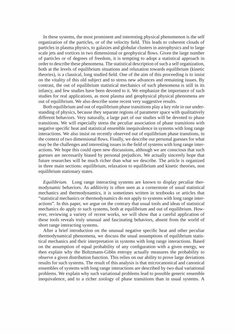


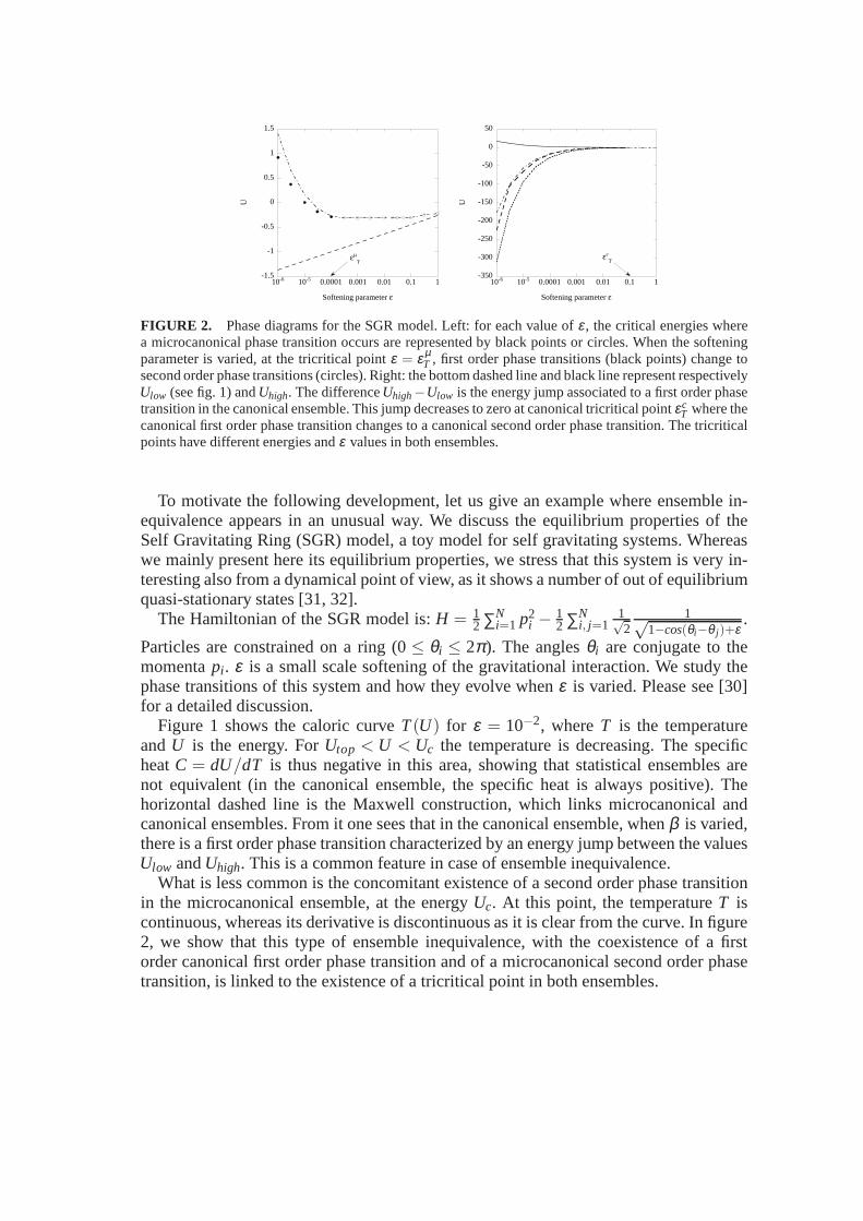


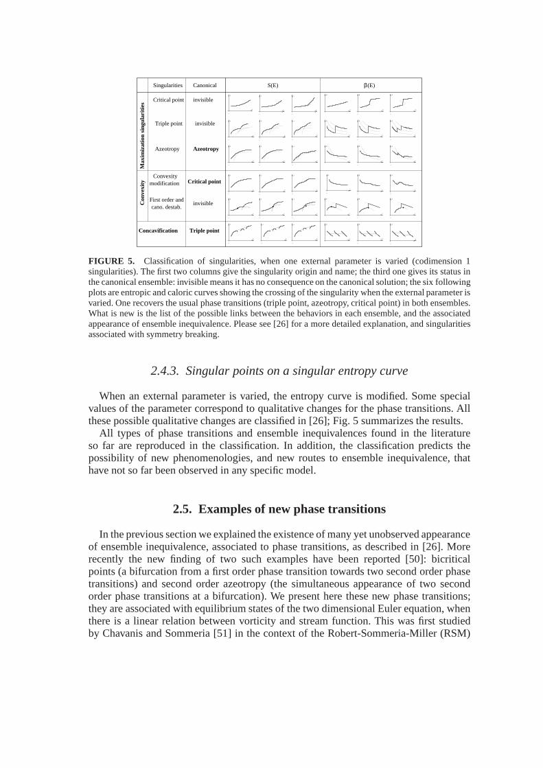


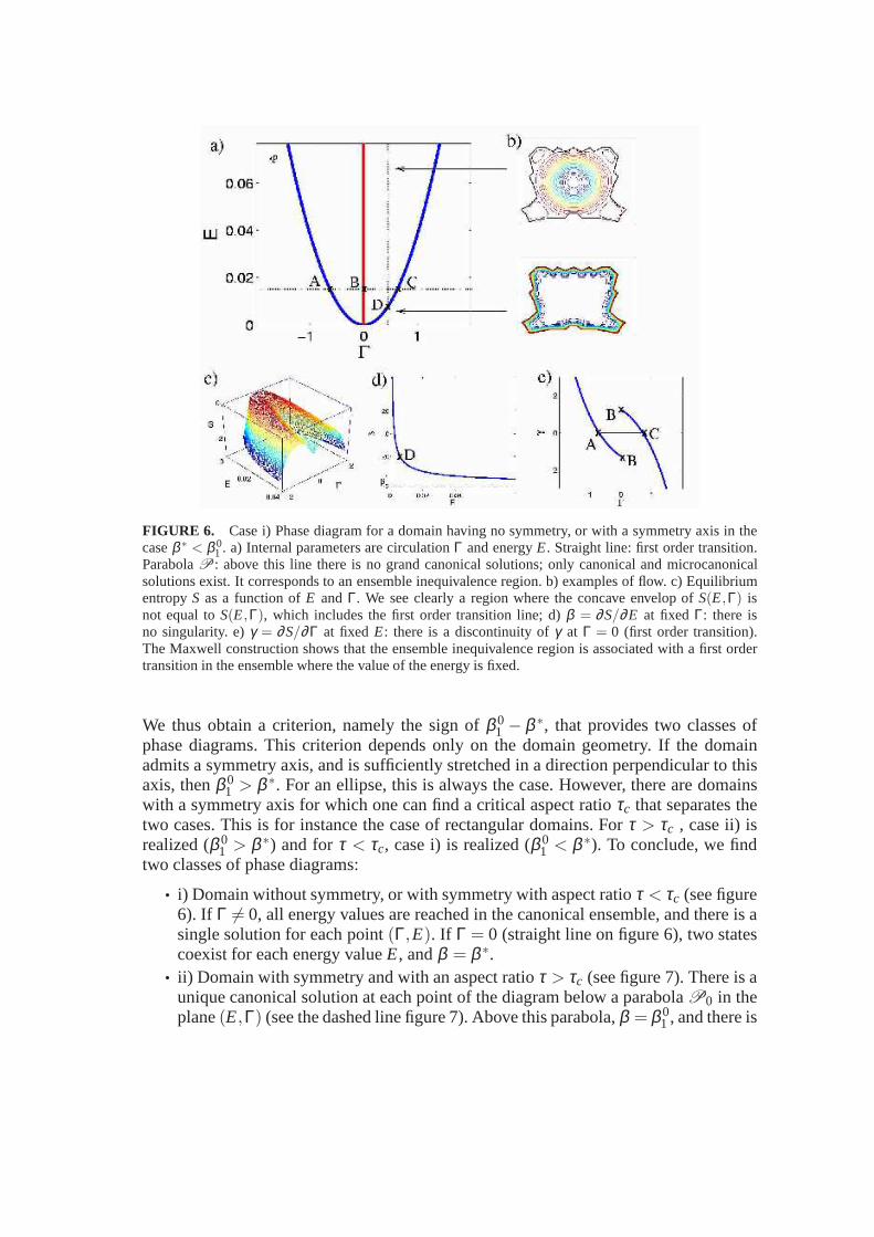
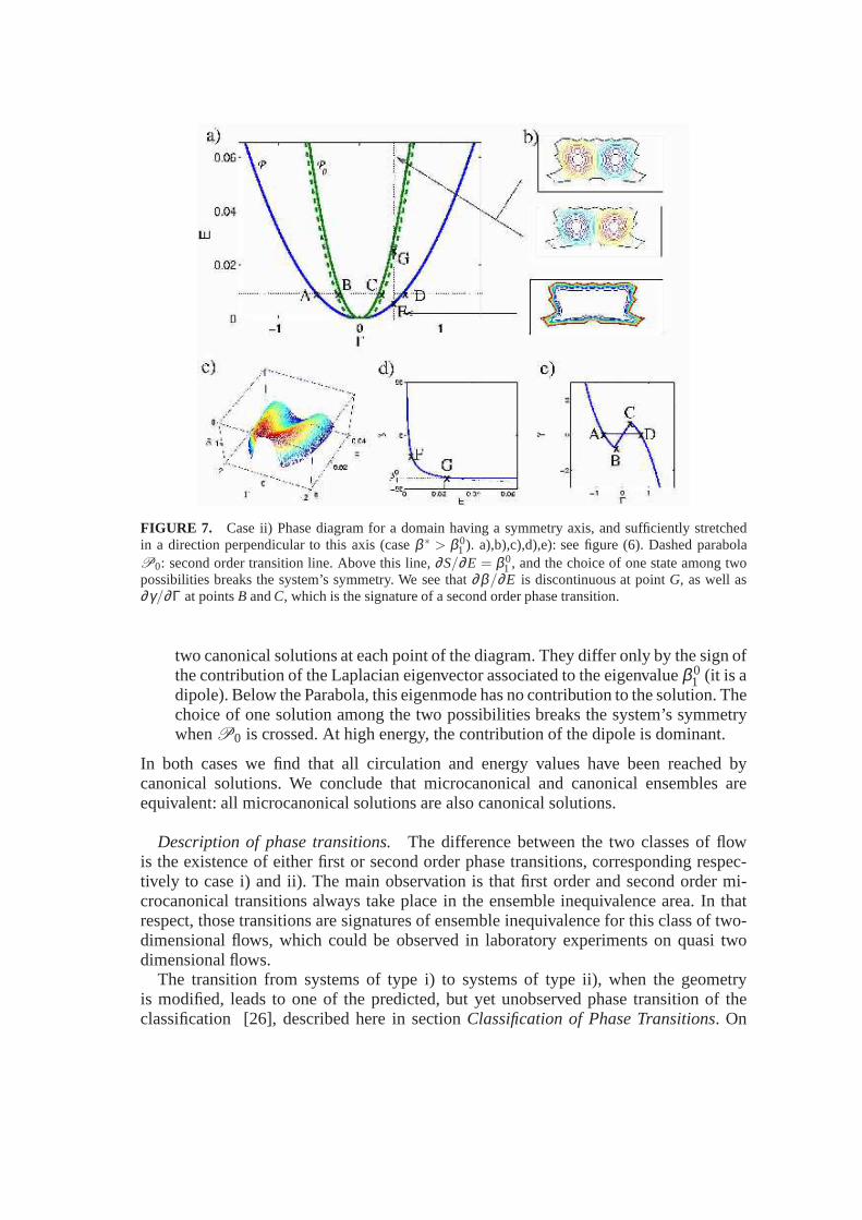
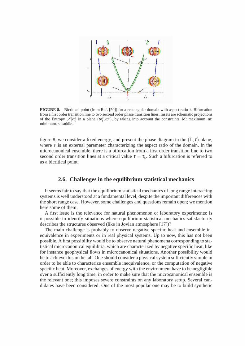


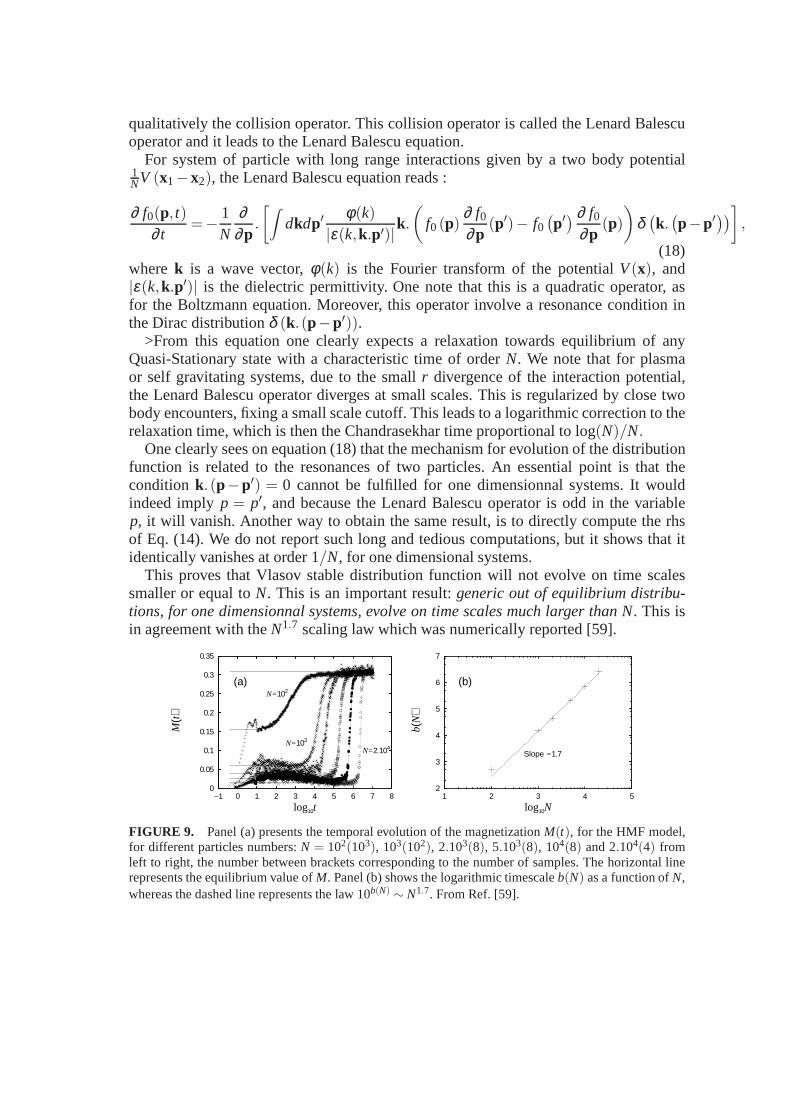


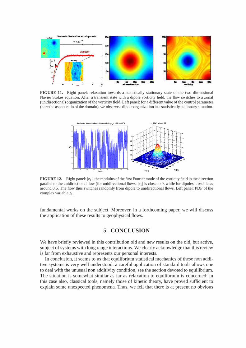
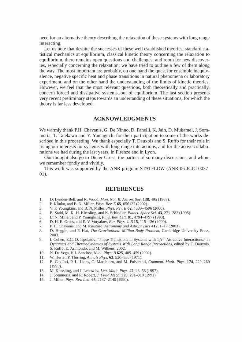


![PAPER: CLASSICAL STATISTICAL MECHANICS, EQUILIBRIUM …vdemery/files/articles/Demery2019.pdf · mation and thermodynamics [ 9] or test out-of-equilibrium extensions of the fluctuation-dissipation](https://static.documents.pub/doc/80x56/5f278a2722ff701f231a92cb/paper-classical-statistical-mechanics-equilibrium-vdemeryfilesarticles-mation.jpg)


