WP/07/296

Equilibrium Exchange Rates: Assessment Methodologies

Peter Isard

© 2007 International Monetary Fund WP/07/296 IMF Working Paper IMF Institute

Equilibrium Exchange Rates: Assessment Methodologies

Prepared by Peter Isard1

December 2007

Abstract

This Working Paper should not be reported as representing the views of the IMF. The views expressed herein are those of the author(s) and should not be attributted to the IMF, its Executive Board, ot its management. Working Papers describe research in progress by the author(s) and are published to elicit comments and to further debate.

The paper describes six different methodologies that have been used to assess the equilibrium values of exchange rates and discusses their limitations. It applies several of the approaches to data for the United States as of 2006, illustrates that different approaches sometimes provide substantially different assessments, and asks which methodologies deserve the most weight in such situations. It argues that while it is generally desirable to consider the implications of several different approaches, since different approaches provide different types of perspectives, two of the methodologies seem particularly relevant for identifying threats to macroeconomic stability and growth. JEL Classification Numbers: F3, F31 Keywords: Equilibrium exchange rates Author’s E-Mail Address: pisard@imf.org

1 I am grateful for helpful comments from Gian Maria Milesi-Ferretti, Jaewoo Lee, Jonathan Ostry, Russell Kincaid, Carlo Cottarelli, and Tam Bayoumi. It should not be assumed that they completely agree with the views expressed in this paper.

2

Contents Page

I. Introduction ............................................................................................................................3

II. The Purchasing Power Parity Approach ...............................................................................5

III. PPP Adjusted for the Balassa-Samuelson and Penn Effects..............................................10

IV. The Macroeconomic Balance Framework.........................................................................14

V. Assessments of the Competitiveness of the Tradable Goods Sector ..................................19

VI. Assessments Based on Estimated Exchange Rate Equations ............................................19

VII. Assessments Based on General Equilibrium Models.......................................................21

VIII. Case Study: The United States........................................................................................22

IX. Which Assessment Methodologies Deserve the Most Weight? ........................................31

X. Conclusions.........................................................................................................................34 Boxes Box 1. The Purchasing Power Parity Hypothesis ......................................................................6 Box 2. PPP and the Balassa-Samuelson Hypothesis ...............................................................11 Box 3. A Simple Model of the Underlying Current Account Balance ....................................17 Figures Figure 1. Exchange Rate Changes Versus Inflation Differentials Over Different Time ...........7 Intervals Figure 2. Real Exchange Rates Between the United Kingdom and Germany, 1970-2000 .......9 Figure 3. Cross-Section Evidence on the Relationship Between ICP Measure of Real ..........13 Exchange Rates and GDP Per Worker Figure 4. Medium-Run Fundamentals ..........................................................................15 Figure 5. Real Effective Exchange Rates: United States, 1980-2006......................................24 Figure 6. Unit Labor Cost and the Implicit Price Deflator for the U.S....................................25 Nonfinancial Corporate Sector, 1995 Q1 – 2006 Q4 Figure 7. After-Tax Profits per Dollar of Sales in U.S. Manufacturing, .................................26 1995Q1 – 2006Q4 Figure 8. U.S. Goods Exports as Percent of GDP, 1995Q1-2006Q4 ......................................27 Figure 9. U.S. Current Account Balance as a Percent of GDP, 1970-2006.............................29 Figure 10. U.S. Net Foreign Assets as Ratio to GDP, 1980-2006...........................................30 Appendix I. Assessing the Sustainability of the Net Foreign Liability Position .....................37 Appendix II. An Estimate of the U.S. Underlying Current Account Position in 2006............39 References ..........................................................................................................................43

3

I. INTRODUCTION

Assessing the equilibrium levels of exchange rates is an important responsibility of macroeconomic policymakers. Exchange rates have a major influence on the prices faced by consumers and producers throughout the world, and the consequences of substantial misalignments can be extremely costly. The currency crises experienced by a number of emerging-market economies over the past decade testify to the large output contractions and extensive economic hardship that can be suffered when exchange rates become badly misaligned and subsequently change abruptly. Moreover, there is reasonably strong evidence that the alignment of exchange rates has a critical influence on the rate of growth of per capita output in low income countries.2 Economists have developed a number methodologies for assessing equilibrium exchange rates. Each methodology involves conceptual simplifications and/or imprecise estimates of key parameters; and different methodologies sometimes generate markedly different quantitative estimates of equilibrium exchange rates. This makes it difficult to place much confidence in estimates derived from any single methodology on its own. By the same token, it suggests that, ideally, policymakers should inform their judgments through the application of several different methodologies. This paper describes six different approaches that economists have used to estimate equilibrium exchange rates in recent years and discusses their pros and cons. The taxonomy of approaches distinguishes between purchasing power parity (addressed in Section II), purchasing power parity adjusted for Balassa-Samuelson and Penn effects (Section III), two variants of the macroeconomic balance framework (Section IV), assessments of the competitiveness of the tradable goods sector (Section V), assessments based on estimated exchange rate equations (Section VI), and assessments based on general equilibrium models (Section VII).3 Four of the methodologies are illustrated using 2006 data for the United States (Section VIII), which is a particularly interesting case because of the dollar’s importance and because the different methodologies generate a wide dispersion of assessments for the U.S. currency. Which of the many approaches should be emphasized when assessing whether exchange rates are badly misaligned (Section IX)? The answer depends on the purpose of the assessment exercise and the resources available. Given its core responsibility for monitoring whether countries’ policies are consistent with a code of conduct that is conducive to external stability and the smooth functioning of the international monetary system, the International Monetary Fund conducts regular assessment exercises that are currently applied to a group of 27 countries4 and informed by at least three of the methodologies, including the two variants 2 See, for example, Johnson, Ostry, and Subramanian (2007).

3 The PPP approaches and estimated exchange rate equations can be regarded as price-based methodologies, while the two variants of the macroeconomic balance approach can be viewed as quantity-based methodologies.

4 The choice of countries has been dictated by both conceptual considerations and the availability of data.

4

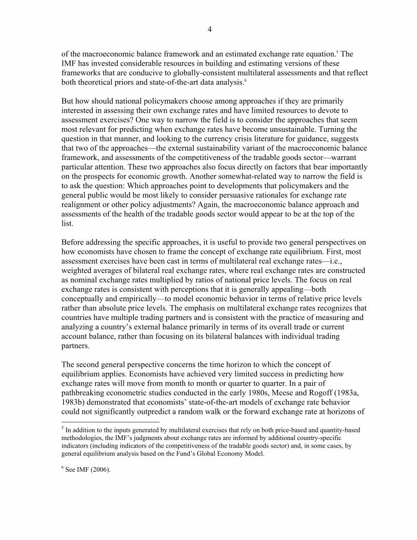
of the macroeconomic balance framework and an estimated exchange rate equation.5 The IMF has invested considerable resources in building and estimating versions of these frameworks that are conducive to globally-consistent multilateral assessments and that reflect both theoretical priors and state-of-the-art data analysis.6 But how should national policymakers choose among approaches if they are primarily interested in assessing their own exchange rates and have limited resources to devote to assessment exercises? One way to narrow the field is to consider the approaches that seem most relevant for predicting when exchange rates have become unsustainable. Turning the question in that manner, and looking to the currency crisis literature for guidance, suggests that two of the approaches—the external sustainability variant of the macroeconomic balance framework, and assessments of the competitiveness of the tradable goods sector—warrant particular attention. These two approaches also focus directly on factors that bear importantly on the prospects for economic growth. Another somewhat-related way to narrow the field is to ask the question: Which approaches point to developments that policymakers and the general public would be most likely to consider persuasive rationales for exchange rate realignment or other policy adjustments? Again, the macroeconomic balance approach and assessments of the health of the tradable goods sector would appear to be at the top of the list. Before addressing the specific approaches, it is useful to provide two general perspectives on how economists have chosen to frame the concept of exchange rate equilibrium. First, most assessment exercises have been cast in terms of multilateral real exchange rates—i.e., weighted averages of bilateral real exchange rates, where real exchange rates are constructed as nominal exchange rates multiplied by ratios of national price levels. The focus on real exchange rates is consistent with perceptions that it is generally appealing—both conceptually and empirically—to model economic behavior in terms of relative price levels rather than absolute price levels. The emphasis on multilateral exchange rates recognizes that countries have multiple trading partners and is consistent with the practice of measuring and analyzing a country’s external balance primarily in terms of its overall trade or current account balance, rather than focusing on its bilateral balances with individual trading partners. The second general perspective concerns the time horizon to which the concept of equilibrium applies. Economists have achieved very limited success in predicting how exchange rates will move from month to month or quarter to quarter. In a pair of pathbreaking econometric studies conducted in the early 1980s, Meese and Rogoff (1983a, 1983b) demonstrated that economists’ state-of-the-art models of exchange rate behavior could not significantly outpredict a random walk or the forward exchange rate at horizons of 5 In addition to the inputs generated by multilateral exercises that rely on both price-based and quantity-based methodologies, the IMF’s judgments about exchange rates are informed by additional country-specific indicators (including indicators of the competitiveness of the tradable goods sector) and, in some cases, by general equilibrium analysis based on the Fund’s Global Economy Model.

6 See IMF (2006).

5

up to 12 months, even when the models were given the benefit of ex post (realized) data on their explanatory variables. Moreover, numerous attempts to overturn that result have had very limited success.7 By contrast, Meese and Rogoff also found (and others have since verified) that at horizons of a few years or more, forward exchange rates and random walk models generate significantly less accurate forecasts than the types of macroeconomic variables that economists tend to focus on when trying to explain the behavior of exchange rates or assess the “equilibrium levels” toward which exchange rates are likely to gravitate. Accordingly, in most applications of the approaches considered in this paper, equilibrium is viewed as a medium-run concept.

II. THE PURCHASING POWER PARITY APPROACH

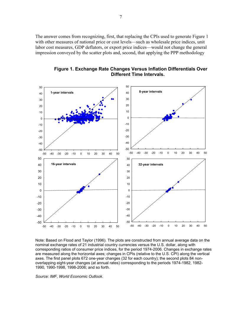
In assessing the level of a real exchange rate, a common first step is to compare the prevailing level with some historical average. Such comparisons often presume that real exchange rates should remain relatively constant over time, or that nominal exchange rates should move in line with ratios of national price levels, consistent with the purchasing power parity (PPP) hypothesis (Box 1). The term “purchasing power parity” was coined by the Swedish economist Gustav Cassel in 1918. Economists at the time faced the issue of suggesting appropriate levels for nominal exchange rates following the abandonment of gold parities at the outset of the First World War and several years in which countries had experienced widely different rates of inflation. Cassel hypothesized that “free movement of merchandise and a somewhat comprehensive trade” would result in parity between the purchasing powers of the moneys of different countries, as indicated by national price levels.8 This was not a new theory. The perception that nominal exchange rates are related to national price levels has been traced at least as far back as the sixteenth century, where its genesis was linked to the development of the quantity theory of money by Spanish economists, who received inspiration from observing the effects on money supplies, price levels, and exchange rates of large inflows of gold from newly-discovered America.9 Empirical support for the PPP hypothesis can be seen in Figure 1, which replicates a chart from Flood and Taylor (1996). The plots are constructed from annual average data on the nominal exchange rates of 21 industrial country currencies against the U.S. dollar for the period 1974-2006, along with corresponding consumer price indices. Percentage changes in

7 See Frankel and Rose (1995) and Rogoff (1999). A notable exception is the success achieved by Chen and Rogoff (2003) for three “commodity currencies” (the Australian, Canadian, and New Zealand dollars). In addition, significant success has been achieved at exploiting micro-structural data on orders and transactions flows to forecast exchange rates at short horizons of up to three weeks; see Evans and Lyons (2002, 2005).

8 Cassel (1918, p. 413). In later writings, Cassel (1922) clarified that he regarded PPP as a central tendency, noting a number of factors that prevented PPP from holding continuously.

9 Einzig (1970) and Officer (1982), who both cite Grice-Hutchinson (1952).

6

Box 1. The Purchasing Power Parity Hypothesis

PPP theory has two main variants. The absolute PPP hypothesis states that the exchange rate between the currencies of two countries should equal the ratio of the price levels of the two countries. Specifically, S = P*/P (1.1) where S is the nominal exchange rate measured in units of foreign currency per unit of domestic currency, P is the domestic price level, and P* is the foreign price level. The relative PPP hypothesis states that the exchange rate should bear a constant proportionate relationship to the ratio of national price levels: in particular, S = kP*/P (1.2) where k is a constant parameter. l/ Either variant implies a constant real exchange rate R = SP/P* (1.3) Note also that the logarithmic transformations of (1.1) and (1.2) have the form s = c + p*- p (1.4) where s, p, p* are the logarithms of S, P, P* and c = log(k) = 0 under absolute PPP. Under either variant of PPP, a change in the ratio of price levels implies an equiproportionate change in the nominal exchange rate, such that ∆s = ∆p* - ∆p (1.5) 1/ Because data on aggregate price levels are generally indexed to base years that may differ across countries, tests of the empirical validity of PPP generally focus on the relative PPP hypothesis. nominal exchange rates are measured along the horizontal axes and percentage changes in ratios of corresponding CPIs along the vertical axes. The top-left panel plots 672 changes over one-year intervals (32 for each of 21 countries); the top-right panel shows 84 changes over non-overlapping eight-year intervals; and so forth. The convergence of the scatter plots toward the diagonal 45 degree lines as the time interval is lengthened—which amounts to mean reversion in real exchange rates—provides very strong support for PPP as a long-run hypothesis, at least for the industrial countries over the past three decades. It is tempting to interpret the gravitational tendency conveyed by Figure 1 as strong support for the simple methodology of defining the equilibrium levels of real exchange rates as their historical average levels over moderately long periods of time. But that begs the question of why economists have felt compelled to develop other approaches for estimating equilibrium exchange rates.

7

The answer comes from recognizing, first, that replacing the CPIs used to generate Figure 1 with other measures of national price or cost levels—such as wholesale price indices, unit labor cost measures, GDP deflators, or export price indices—would not change the general impression conveyed by the scatter plots and, second, that applying the PPP methodology

Figure 1. Exchange Rate Changes Versus Inflation Differentials Over Different Time Intervals.

Note: Based on Flood and Taylor (1996). The plots are constructed from annual average data on the nominal exchange rates of 21 industrial country currencies versus the U.S. dollar, along with corresponding ratios of consumer price indices, for the period 1974-2006. Changes in exchange rates are measured along the horizontal axes; changes in CPIs (relative to the U.S. CPI) along the vertical axes. The first panel plots 672 one-year changes (32 for each country); the second plots 84 non-overlapping eight-year changes (at annual rates) corresponding to the periods 1974-1982, 1982-1990, 1990-1998, 1998-2006; and so forth. Source: IMF, World Economic Outlook.

1-year intervals

-50 -40 -30 -20 -10

0 10 20 30 40 50

-50 -40 -30 -20 -10 0 10 20 30 40 50

8-year intervals

-50

-40

-30

-20

-10

0

10

20

30

40

50

-50 -40 -30 -20 -10 0 10 20 30 40 50

16-year intervals

-50 -40 -30 -20 -10

0 10 20 30 40 50

-50 -40 -30 -20 -10 0 10 20 30 40 50

32-year intervals

-50

-40

-30

-20

-10

0

10

20

30

40

50

-50 -40 -30 -20 -10 0 10 20 30 40 50

8

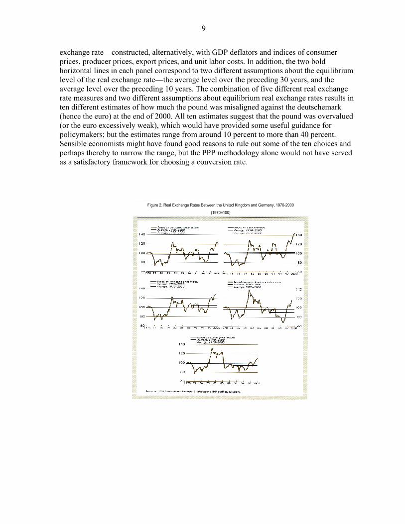
with different choices of price or cost indices can yield very different estimates of equilibrium exchange rates. Indeed, one of the most famous and disastrous applications of the PPP approach—the analysis that guided the British return to the gold standard in April 1925—involved an unfortunate or misguided choice between two different sets of PPP calculations. As of early 1925, the nominal exchange rate of the pound was close to its prewar parities against the U.S. dollar and gold, and data on British and American wholesale prices suggested that the ratio of national price levels had changed by only two or three percent since the prewar period. Application of the PPP methodology using wholesale price indices thus supported a return to gold at the prewar parity—the choice that was ultimately made by Winston Churchill, then Chancellor of the Exchequer. By contrast, the PPP methodology had also led John Maynard Keynes to testify to a parliamentary committee that the pound would be 12 percent overvalued at that parity, based on a comparison of British and American retail prices.10 Churchill had consulted with Keynes, but either was not persuaded that British workers would have to accept large real wage cuts or misunderstood or underrated the consequences for unemployment and industrial strife.11 It can be argued, in retrospect, that sound economic analysis pointed clearly to the better choice, and that Churchill’s mistake was that he failed to listen to sensible economists. Indeed, soon after the April 1925 decision, in an essay castigating Churchill’s advisors, Keynes emphasized that the prevailing wholesale price indices were “made up ... at least two-thirds from the raw materials of international commerce, the prices of which necessarily adjust themselves to the exchanges ... [I]ndex numbers of the cost of living, of the level of wages, and of the prices of our manufactured exports ... are a much better rough-and-ready guide.”12 Even so, it is not always easy to identify the best choice among several different PPP-based estimates of equilibrium exchange rates. Consider, for example, the hypothetical question of what conversion rate would have been most appropriate if the United Kingdom had been scheduled to adopt the euro at the end of 2000. Figure 213 uses the PPP methodology to generate a wide range of answers based on the history of real exchange rates between the pound and the deutschemark. Each of the five panels shows a different measure of the real

10 Moggridge (1972).

11 Descriptions of the disastrous consequences include the allegation that the erosion of British competitiveness and the difficulties of tightening British monetary policy to stem the associated outflow of gold induced the United States to keep monetary policy easier than it would otherwise have been during the second half of 1927 and unintentionally contributed to the boom and bust on Wall Street; see Yeager (1976, p. 336).

12 Keynes (1925, p. 11). Nurkse (1944, p. 128) notes that the British mistake was repeated by Czechoslovakia in 1934, when the currency was devalued by 16 percent on the basis of inappropriate PPP calculations and required a second devaluation two years later.

13 This replicates Figure 3 from Isard and others (2001).

9

exchange rate—constructed, alternatively, with GDP deflators and indices of consumer prices, producer prices, export prices, and unit labor costs. In addition, the two bold horizontal lines in each panel correspond to two different assumptions about the equilibrium level of the real exchange rate—the average level over the preceding 30 years, and the average level over the preceding 10 years. The combination of five different real exchange rate measures and two different assumptions about equilibrium real exchange rates results in ten different estimates of how much the pound was misaligned against the deutschemark (hence the euro) at the end of 2000. All ten estimates suggest that the pound was overvalued (or the euro excessively weak), which would have provided some useful guidance for policymakers; but the estimates range from around 10 percent to more than 40 percent. Sensible economists might have found good reasons to rule out some of the ten choices and perhaps thereby to narrow the range, but the PPP methodology alone would not have served as a satisfactory framework for choosing a conversion rate.

Figure 2. Real Exchange Rates Between the United Kingdom and Germany, 1970-2000

(1970=100)

10

III. PPP ADJUSTED FOR THE BALASSA-SAMUELSON AND PENN EFFECTS

An important modification of the PPP approach has come from the observation that the prices of nontradable goods and services, relative to prices of tradables, tend to be lower in low-income countries than in high-income countries. Confirmation of this empirical regularity, which Samuelson (1994) has coined “the Penn effect,” emerged from attempts to make quantitative cross-country comparisons of standards of living in a series of projects sponsored by the United Nations and other international organizations. These studies, known as the International Comparisons Program (ICP) and spearheaded to a large extent by economists from the University of Pennsylvania,14 have established that the methodology of comparing living standards by using market exchange rates to convert national accounts data into a common currency unit generally understates the living standards of low-income countries relative to those of high-income countries.15 A widely-cited explanation for the Penn effect, generally associated with Balassa (1964) and Samuelson (1964), conjectures that the tendency for the relative price of nontradables to be higher in high income countries comes from a tendency for productivity in the tradable goods sector to rise faster than productivity in the nontradables sector as economies develop and real incomes grow.16 Given competitive pressures within countries for workers with similar skills to receive similar wages in the two sectors, relatively rapid productivity growth in the tradables sector, other things equal, would tend to push up the relative cost of production in the nontradables sector and, hence, the relative price of nontradables. In addition to suggesting an explaination for the Penn effect, the Balassa-Samuelson hypothesis—when combined with the assumption that the prices of tradable goods, converted into a common currency unit, are similar across countries—suggests a tendency for real exchange rates constructed from aggregate national price indices (i.e., indices that reflect the prices of both tradables and nontradables) to appreciate over time for relatively fast growing countries and depreciate for relatively slow growing countries (Box 2). The Balassa-Samuelson hypothesis and its implication for exchange rates focus on the associations between growth over time in national output per capita, the relative levels of per 14 See, for example, Gilbert and Kravis (1954), Kravis, Heston, and Summers (1982), and Summers and Heston (1991).

15 The ICP, established in 1968, has collected data during a number of survey years (starting in 1970) on expenditures and prices in many countries for many detailed categories of goods and services. Quantity data are constructed by dividing expenditures by prices, a system of equations has been developed to generate an “international price” for each product, interpolation and extrapolation methods have been devised for countries and years not covered by the surveys, and GDP and other national accounts aggregates constructed with international price data are now published regularly in the “Penn World Tables” and used by the IMF and other international organizations for purposes of cross country comparisons.

16 The seeds of the Balassa-Samuelson hypothesis can also be found in Harrod (1939) and traced back to Ricardo in 1821 (see Ricardo, 1951).

11

Box 2. PPP and the Balassa-Samuelson Hypothesis

Let

1-

N T N T TP = P P = (P /P ) Pα α α (2.1)

* *β *1-β * * β *

N T N T TP = P P = (P /P ) P (2.2) where TP and NP denote the prices of tradable and nontradable goods in country A; *

TP and *

NP are the corresponding prices in country B; and P and P* are the aggregate price levels in the two countries. Let S be the nominal exchange rate in currency B per unit currency A, and let R denote the real exchange rate R = SP/P* (2.3) Substitution of (2.1) and (2.2) into (2.3) implies * * *

T T N T N TR = S(P /P )(P /P ) /(P /P )α β (2.4) Now consider the Balassa-Samuelson hypothesis, which conjectures that relatively fast growing countries experience relatively rapid productivity growth in the tradables sector accompanied by relatively large increases in the ratio of nontradables prices to tradables prices. Under this hypothesis, if country A grows faster than country B—and under the assumptions that S *

T TP /P remains constant and that any difference between α and β has second-order effects—the value of R will increase over time, implying a real appreciation of currency A. capita outputs in the tradable and nontradable sectors, the relative prices of tradables and nontradables, and the real exchange rate. Several studies have investigated these associations using time series data for OECD countries and Asia-Pacific economies.17 These studies have found strong associations between relative productivity levels and the relative prices of tradables and nontradables; and other things equal, changes in the relative prices of tradables and nontradables give rise to systematic changes in real exchange rates when real exchange 17 Examples of studies based on OECD data include Froot and Rogoff (1995), De Gregorio, Giovannini, and Krueger (1994), De Gregorio, Giovannini and Wolf (1994), Asea and Mendoza (1994), Canzoneri, Cumby, and Diba (1999), and Lee and Tang (2007). Isard and Symansky (1996) provide a study based on data for Asia-Pacific economies and De Broeck and Slok (2001) for a group of 25 transition countries.

12

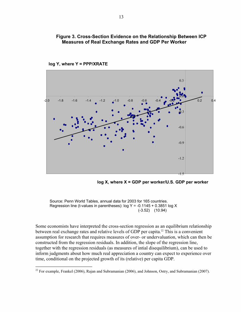
rates are constructed using indices of the aggregate prices of tradables and nontradables.18 Nevertheless, except for a subset of the transition countries,19 the time series data challenge the notion that relatively rapid economic growth generally gives rise to real exchange rate appreciation, suggesting that if productivity growth in the tradables sector is indeed relatively rapid, the implications for exchange rates are often counterbalanced over time by other developments. For example, as Isard and Symansky (1996) document, among the seven Asian economies that grew more rapidly than Japan over the period 1973-1992, only Korea and Taiwan experienced significant real appreciations while Indonesia, Malaysia, and Thailand experienced substantial depreciations and Hong Kong and Singapore very small appreciations. The weak link in the Balassa-Samuelson hypothesis, as applied to real exchange rates, is the assumption that the relative prices of tradable-goods across countries remain relatively constant over time. Indeed, the data show substantial cumulative changes over time in the relative prices of tradable goods across countries when prices are measured at the sectoral level (e.g, when the price of tradable goods is assumed to correspond to an index of prices for the manufacturing sector).20 One likely part of the explanation is that the composition of tradable goods production tends to change over time; as countries develop, their production activities tend to shift toward more sophisticated technologies and higher quality products. Another likely part of the explanation comes from changes in the relative prices of different categories of tradable goods interacting with differences across countries in the weights of the different goods in the price indices of different countries. And a third possibility is that tradable goods prices in different countries are impacted differently by changes over time in the costs of “goods arbitrage,” reflecting changes in transportation (or distribution) costs or the liberalization of trade restrictions. Although the time series data cast doubt on the validity of the Balassa-Samuelson hypothesis as applied to real exchange rates, cross-section data provide evidence of a strong systematic association between real exchange rates and GDP per capita. This can be seen in Figure 3, which is based on ICP data for 2003.21 The latter evidence is appropriately regarded as a straightforward implication of the Penn effect, independently of whether the Balassa-Samuelson hypothesis is a valid explanation of that empirical regularity.

18 See Choudhri and Khan (2005) for a recent panel-data study that provides evidence of these linkages in developing countries.

19 The European Union accession countries; see De Broeck and Slok (2001).

20 There is also a substantial body of literature that rejects the “law of one price” for many specific products and highly disaggregated categories of goods.

21 The real exchange rate measured along the vertical axis is constructed by dividing each country’s nominal exchange rate against the numeraire currency (in domestic currency per U.S. dollar) into the country’s PPP (i.e., its price level in domestic currency units divided by the cost of the same bill of goods at international prices measured in U.S. dollars).

13

Figure 3. Cross-Section Evidence on the Relationship Between ICP

Measures of Real Exchange Rates and GDP Per Worker

Source: Penn World Tables, annual data for 2003 for 165 countries. Regression line (t-values in parentheses): log Y = -0.1145 + 0.3851 log X

(-3.52) (10.94) Some economists have interpreted the cross-section regression as an equilibrium relationship between real exchange rates and relative levels of GDP per capita.22 This is a convenient assumption for research that requires measures of over- or undervaluation, which can then be constructed from the regression residuals. In addition, the slope of the regression line, together with the regression residuals (as measures of intial disequilibrium), can be used to inform judgments about how much real appreciation a country can expect to experience over time, conditional on the projected growth of its (relative) per capita GDP. 22 For example, Frankel (2006), Rajan and Subramanian (2006), and Johnson, Ostry, and Subramanian (2007).

-1.5

-1.2

-0.9

-0.6

-0.3

0.0

0.3

-2.0 -1.8 -1.6 -1.4 -1.2 -1.0 -0.8 -0.6 -0.4 -0.2 0.2 0.4

log Y, where Y = PPP/XRATE

log X, where X = GDP per worker/U.S. GDP per worker

14

IV. THE MACROECONOMIC BALANCE FRAMEWORK

The macroeconomic balance (MB) framework focuses on the requirements for achieving internal and external balance simultaneously. Its origins have been traced back to Nurkse (1945) and Metzler (1951), with pathbreaking contributions from Meade (1951) and Swan (1963), who put the simultaneous balance paradigm on center stage in open economy macroeconomics. Policy analysis based on the MB framework—here defined as the application of the simultaneous balance framework to the assessment of exchange rates—dates back at least to the mid-1960s, when it was employed at the IMF to assess the appropriate size of the prospective devaluation of the British pound. The MB framework has three basic components: an identity with the current account balance on one side; an estimate of the equilibrium value of the terms on the other side of the identity, which typically are assumed to be independent of the real exchange rate; and a relationship between the current account, the real exchange rate, and the levels of the domestic and foreign output gaps. Until the mid-1990s, applications of the MB framework, as refined by IMF economists23 and given prominence by Williamson (1985), were typically based on the balance of payments identity between the current account position (CUR) and the net flow of private and official capital (CAP):

CUR = CAP. (1)

These applications tended to make assumptions about “normal” or “target” or “underlying” levels of net capital flows, which were implicitly associated with positions of internal balance and served as estimates of the equilibrium value of CAP. More recent applications of the MB framework have shifted orientation to the national income accounting identity that links the current account position to the excess of domestic saving (S) over domestic investment (I):24

CUR = S – I. (2)

As elaborated below, two different approaches have been used for estimating equilibrium values for S-I. In applying the MB framework, it is useful to define the concept of the underlying current account position (UCUR) as the value of CUR that would be observed at the prevailing real exchange rate if all countries were operating at full employment or potential output (internal balance) and if the effects of past exchange rate changes had been completely realized. This is the appropriate concept of the medium-run current account position associated with the prevailing real exchange rate—a concept that adjusts for the business cycle and recognizes 23 Artus (1978), Artus and Knight (1984).

24 The relevant measure of CUR depends on the choice of identity. In particular, remittances (transfers) and payments and receipts for factor services are treated differently in the balance of payments accounts and national income accounts.

15

that the effects of changes in the exchange rate on the volumes and values of imports and exports generally take some time to materialize fully. Figure 425 provides a summary picture of the MB framework. The negatively-sloped line depicts a reduced-form relationship between the underlying current account and the real exchange rate, where an increase in the real exchange rate, measured along the vertical axis, corresponds to an appreciation of the domestic currency. Real appreciation generally leads to a decline in the value of exports and an increase in the value of imports, implying a decline in the current account—hence, the negative slope. The bold vertical line represents the equilibrium level of S-I, which is here assumed to be independent of the real exchange rate.26 In general, the positions of both the UCUR line and the S-I line will depend on the values of a number of explanatory variables not shown in the diagram.

Figure 4. Medium-Run Fundamentals

Chart 3. Medium-Run Fundamentals R1 R* UCUR Deficit 0 UCUR1 Surplus

Current account

Equilibrium saving-investment balance

Underlying current account balance

Real effective exchange rate

S-I

The intersection of the UCUR and S-I lines determines the equilibrium value of the real exchange rate (R*). The calculation of R* starts from estimates of (i) the underlying current account position (UCUR1) associated with the prevailing value of the real exchange rate (R1)

25 This replicates Figure 2.2 from Isard and Faruqee, eds. (1998).

26 Relaxing this assumption would not greatly complicate the MB methodology but would raise the more formidable challenge of identifying a stable empirical relationship between the S-I balance and the real exchange rate. In practice, application of the MB approach involves estimates of the equilibrium S-I balance derived from the current or projected values of a number of explanatory variables, some of which may be sensitive to exchange rates.

16

and (ii) the gap between the equilibrium level of S-I and UCUR1. The slope of the UCUR line is then used to estimate how much R would have to change to close the gap, other things equal.27 Estimation of the UCUR balance requires a model of the current account. Many countries have developed such models. The most appealing specifications and calibrations tend to be country-specific, reflecting factors such as country size and the composition of exports and imports. For that reason it would not be attractive to use a common model specification for all countries, which is recognized in applications at the IMF.28 For purposes of illustration, however, it may be helpful to consider a skeletal model and how it would be used to estimate the UCUR position. Box 3 describes the calculation of UCUR based on a streamlined model of net exports—i.e., the current account as defined in the national income accounts. Imports (M) depend on the current level of domestic economic activity (Y), where activity is typically measured by GDP, as well as on the history of the real exchange rate (R) extending back several calendar quarters. (It typically takes at least one to two years—represented in the Box as n calendar quarters—for exchange rate changes to have their full effects on the volumes of imports and exports.) Exports (X) depend symmetrically on a trade-weighted average of foreign economic activity and the history of real exchange rates. And from the given specifications of the import and export equations, it is straightforward to calculate the underlying levels of imports M)( , exports X),( and the current account (net exports) as the levels that would prevail at the full-employment or potential-output levels of domestic and foreign activity if the effects of past exchange rate changes had been completely realized—i.e., if at least n calendar quarters had elapsed since the real exchange rate reached its prevailing level. Estimation of the equilibrium S-I position poses a greater challenge than estimation of the UCUR balance. Two approaches have been taken. One relies on econometric estimates of the relationship between the S-I balance and a list of relevant explanatory variables; the equilibrium S-I position is calculated from the estimated relationship based on assumptions about the equilibrium values of the explanatory variables. The second approach starts from an assumption about the equilibrium stock and composition of net foreign assets (liabilities)

27 Because an n-country world has only n-1 independent exchange rates, it is not possible to conduct the exercise depicted in Figure 4 independently for each country without imposing a mathematical requirement for global consistency. A general procedure for adjusting the individual country calculations to produce a set of globally consistent calculations is described by Faruqee (1998). When the sum across countries of the estimated underlying current account positions is within a few percent of the sum of the estimated equilibrium S-I levels, the required adjustments are generally quite small.

28 The multilateral assessment exercises conducted by the IMF take estimates of UCUR from the medium-term projections that are generated in the World Economic Outlook (WEO) exercise under the assumptions that output gaps close and real exchange rates remain unchanged. The WEO exercise iterates to obtain approximate global consistency, and the current account projections are based on different models for different countries, reflecting area department views on the most appropriate specification and calibration for each country.

17

and defines the equilibrium S-I position as the balance of the associated investment income flows and capital gains and losses.

Box 3. A Simple Model of the Underlying Current Account Balance

A common skeletal framework for modeling the current account and its underlying position is ( )= , , . . . t t t t-nM M Y R R (3.1)

( )*

t t t t-nX X Y ,R ,...R= (3.2)

t t tCUR X M= − (3.3) ( )t t t tM M Y R ,...R,= (3.4)

( )*t t t tX X Y , R ,...R= (3.5)

t t tUCUR X M= − (3.6) where M = imports X = exports Y, Y* = domestic and foreign GDP

*

Y Y, = full-employment or potential-output levels of GDP R = the real exchange rate and an increase in R represents an appreciation of the domestic currency. Appendix II uses a calibrated variant of this skeletal model, as adapted from Bayoumi and Faruqee (1998), to estimate the UCUR position for the United States. In general, however, it is preferable to use a more elaborated empirically-estimated model of a country’s current account when such a model is available.

18

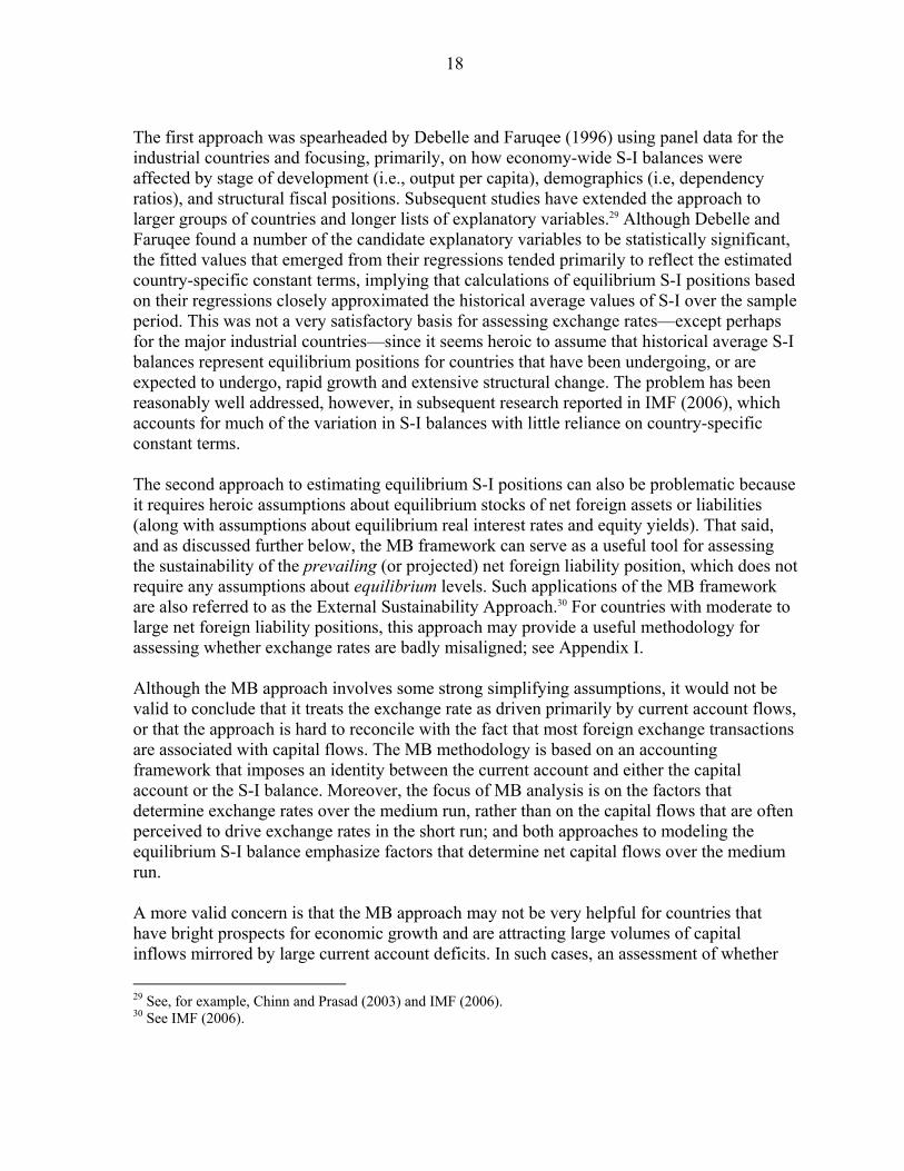
The first approach was spearheaded by Debelle and Faruqee (1996) using panel data for the industrial countries and focusing, primarily, on how economy-wide S-I balances were affected by stage of development (i.e., output per capita), demographics (i.e, dependency ratios), and structural fiscal positions. Subsequent studies have extended the approach to larger groups of countries and longer lists of explanatory variables.29 Although Debelle and Faruqee found a number of the candidate explanatory variables to be statistically significant, the fitted values that emerged from their regressions tended primarily to reflect the estimated country-specific constant terms, implying that calculations of equilibrium S-I positions based on their regressions closely approximated the historical average values of S-I over the sample period. This was not a very satisfactory basis for assessing exchange rates—except perhaps for the major industrial countries—since it seems heroic to assume that historical average S-I balances represent equilibrium positions for countries that have been undergoing, or are expected to undergo, rapid growth and extensive structural change. The problem has been reasonably well addressed, however, in subsequent research reported in IMF (2006), which accounts for much of the variation in S-I balances with little reliance on country-specific constant terms. The second approach to estimating equilibrium S-I positions can also be problematic because it requires heroic assumptions about equilibrium stocks of net foreign assets or liabilities (along with assumptions about equilibrium real interest rates and equity yields). That said, and as discussed further below, the MB framework can serve as a useful tool for assessing the sustainability of the prevailing (or projected) net foreign liability position, which does not require any assumptions about equilibrium levels. Such applications of the MB framework are also referred to as the External Sustainability Approach.30 For countries with moderate to large net foreign liability positions, this approach may provide a useful methodology for assessing whether exchange rates are badly misaligned; see Appendix I. Although the MB approach involves some strong simplifying assumptions, it would not be valid to conclude that it treats the exchange rate as driven primarily by current account flows, or that the approach is hard to reconcile with the fact that most foreign exchange transactions are associated with capital flows. The MB methodology is based on an accounting framework that imposes an identity between the current account and either the capital account or the S-I balance. Moreover, the focus of MB analysis is on the factors that determine exchange rates over the medium run, rather than on the capital flows that are often perceived to drive exchange rates in the short run; and both approaches to modeling the equilibrium S-I balance emphasize factors that determine net capital flows over the medium run. A more valid concern is that the MB approach may not be very helpful for countries that have bright prospects for economic growth and are attracting large volumes of capital inflows mirrored by large current account deficits. In such cases, an assessment of whether 29 See, for example, Chinn and Prasad (2003) and IMF (2006). 30 See IMF (2006).

19

the exchange rate is badly misaligned requires considerable judgment that takes into account, among other things, the degree to which the capital inflows are supporting productive investments and conducive to a shift over time in the current account position. It may be helpful to illustrate the key ingredients and assumptions involved in using the MB framework by working through a specific application. This is done in Section VIII below.

V. ASSESSMENTS OF THE COMPETITIVENESS OF THE TRADABLE GOODS SECTOR

The MB framework focuses on a country’s current account position and embodies a concept of equilibrium that takes an economy-wide perspective. Another approach is to look more narrowly at the performance of the tradable goods sector of the economy and ask how well it is competing at the prevailing real exchange rate. There are different ways to define the tradable goods sector and different ways to assess its competitiveness, as illustrated in Section VIII below. Ideally, the assessments should focus on a range of indicators, exploiting whatever relevant data are available. Many countries generate data on the performance of the manufacturing sector, which is often taken to represent the tradable goods sector. Commonly-used indicators of competitiveness include measures of profitability, trends in export volumes or shares of world exports, and trends in import penetration ratios. Where direct data on profit rates are not available, profitability can sometimes be inferred from data on unit labor costs and value-added deflators, as illustrated by Lipschitz and McDonald (1992). Their analysis of Italy’s international competitiveness, based on trends in sectoral data on unit labor costs and prices, emphasizes that the impression one gets from simply looking at trends in real exchange rates can sometimes be badly misleading. In particular, their study notes that despite the substantial real appreciation of the Italian lira against the Deutschemark between 1979 and 1988, the ratio of unit labor costs to price (value-added deflator) in Italian manufacturing fell relative to the corresponding ratio in Germany, suggesting that Italy’s tradable goods sector gained competitiveness over that period relative to German manufacturers.

VI. ASSESSMENTS BASED ON ESTIMATED EXCHANGE RATE EQUATIONS

The decade that followed the breakdown of the Bretton Woods System in 1971 gave rise to “a ‘heroic age’ of exchange rate theory”31 and to many econometric estimates of reduced-form exchange rate equations. International economists engaged in a spirited competition to explain the observed behavior of exchange rates, focusing on three different structural frameworks for modeling them—flexible price monetary models, sticky-price monetary models, and the portfolio balance framework.32 Many empirical efforts generated 31 Krugman (1993, p. 6).

32 See Isard (1995) and Frankel and Rose (1995) for surveys.

20

statistically-significant coefficients with theoretically-correct signs as well as impressive in-sample goodness-of-fit statistics. The heroic age ended after Meese and Rogoff (1983a, 1983b) conducted an extensive set of carefully-designed tests using state-of-the-art versions of the range of structural models and found that none of the structural models could outperform a random walk in predicting exchange rates between the major industrial currencies out-of-sample at horizons of up to one year.33 As noted earlier, numerous attempts to overturn the Meese-Rogoff results have achieved only limited success. Moreover, as emphasized by Flood and Rose (1999), the short-run volatility of the exchange rate far exceeds the volatility of the macroeconomic fundamentals that economists have suggested as explanatory variables, implying that economists should not hope to achieve much success in attempting to explain the short-run behavior of exchange rates in terms of fundamentals alone.34 Such findings, however, pertain only to the explanatory power of reduced-form exchange rate models at short horizons. As is true of the PPP hypothesis, reduced-form models (many of which nest the PPP hypothesis) may have much greater validity at medium-run and long-run horizons. Advances in econometric methodology since the early 1980s—in particular, the introduction of the concept of cointegration by Granger (1981) and Engel and Granger (1987) and the subsequent development of time series econometrics—have provided new techniques for seeking to empirically estimate the long-run relationship between exchange rates and other economic fundamentals. This has led Faruqee (1995) and others to develop models that focus simultaneously on long-run equilibrium conditions for both asset stocks and current account flows (more generally, national income account flows) in the spirit of Mussa (1984).35 These studies embody PPP not as a time-invariant level of the long-run real exchange rate, but rather as a fixed steady-state condition in which the equilibrium level of the real exchange rate is viewed to depend on the steady-state levels of various fundamental determinants. Faruqee’s empirical work found that the multilateral real exchange rate for the United States was linked, over the long run, to the U.S. net foreign asset position and the rate of U.S. productivity growth (relative to that in other major industrial countries). It also showed that various measures of productivity growth in Japan shared a long-run relationship with Japan’s real exchange rate. At the stage of empirical implementation, this approach to exchange rate modeling typically involves the estimation of single-equation reduced-form error-correction specifications.36 For

33 Engel, Mark, and West (2007) argue that out-of-sample fit is too harsh a criterion for exchange rate models. Rogoff (2007) provides a rejoinder.

34 Rogoff (1999) provides concise perspectives. The short-run volatility of equity prices also far exceeds the volatility of relevant fundamentals.

35 Faruqee (1995) considered a world with two countries engaging in trade in two distinct goods and one financial asset—a continuous-time version of the stock-flow consistent framework described by Mussa (1984).

36 Some studies have estimated vector-equation models.

21

modelers who adhere to the approach described by Mussa (1984) and Faruqee (1995), the reduced-form specification is derived by requiring long-run saving-investment equilibrium to be consistent with an equilibrium net foreign asset (NFA) position, and by combining the long-run condition on the saving-investment balance (which equals the current account) with a model relating the time path of the current account—and hence the change in the NFA position—to the timepath of the real exchange rate. This framework suggests looking for a long-run (cointegrating) relationship between the real exchange rate, the net foreign asset position, and variables that the influence the level of the current account associated with a given level of the real exchange rate. For example, the long-run exchange rate equation reported in IMF (2006) includes as explanatory variables the net foreign asset position (as a ratio to the average of exports and imports), the difference between productivity (output per worker) in the tradables and nontradables sectors relative to trading partners, a measure of the commodity terms of trade (based on country-specific weights), the level of government consumption (as a ratio to GDP), a trade restriction index, and a measure of the extent of price controls (the share of administered prices in the CPI basket). Exchange rate regressions are widely used in exchange rate modeling by many central banks and market participants. When properly specified and estimated, they represent the state-of-the-art approach to data analysis and can serve as useful benchmarks for assessing the relationships between the exchange rate and relevant explanatory variables. Moreover, to the extent that they nest the PPP hypothesis, they can be viewed as the most general price-based approach to exchange rate assessment, which provides an important complement to the two variants of the quantity-based macroeconomic balance approach. Neeedless to say, the value of this approach for informing judgments about equilibrium exchange rates depends on how well the regression results conform to theoretical priors about variables that ought to have significant explanatory power, as well as on whether the estimated coefficients on those variables are consistent with prior beliefs about their signs and approximate magnitudes. And while the current generation of estimated exchange rate equations has more solid conceptual underpinnings than the equations estimated in the 1970s and early 1980s, the use of regressions to generate estimates of the equilibrium values of exchange rates requires assumptions about the equilibrium values of the explanatory variables, which for some variables—in particular, the net foreign asset position—are subject to considerable uncertainty.

VII. ASSESSMENTS BASED ON GENERAL EQUILIBRIUM MODELS

In principle, estimates of equilibrium exchange rates derived from general equilibrium models are preferable to estimates generated under other approaches. Unlike reduced-form regressions and the partial equilibrium models embedded in the macroeconomic balance framework, general equilibrium models provide a more complete representation of macroeconomic behavior, impose important accounting identities, and generate solutions (forecasts) for endogenous variables that are consistent with those identities. In practice, however, complete macroeconomic models are only available for a limited number of countries. Moreover, many of the macroeconomic models that are available have been designed for purposes of short-term forecasting and do not have carefully specified long-run

22

properties, which limits their appropriateness for analyzing the long-run relationships between the exchange rate and other economic fundamentals. Although few in number, those simulation studies that have looked at the behavior of exchange rates through the lens of well-specified general equilibrium models provide important perspectives about the limitations of other approaches and the inherent imprecision and ambiguity of any estimates of equilibrium exchange rates.37 One obvious perspective is that the solution (forecast) paths for exchange rates and other endogenous variables are conditional on the forecasts for exogenous variables and the calibrations of many parameters. A related perspective is that the solution paths can also depend importantly on various assumed “shocks” that are imposed to insure that the model is capable of replicating the observed initial positions and recent historical behavior of key macroeconomic variables.38 A third perspective is that the time paths of future exchange rates can be quite sensitive to assumptions about the persistence of the shocks that are assumed to have occurred in the past, and similarly, to the nature of any future shocks that influence the transition to long-run equilibrium. These perspectives underscore that no approach to assessing equilibrium exchange rates—general equilibrium or otherwise—can generate precise estimates of equilibrium levels without making many explicit or hidden assumptions.

VIII. CASE STUDY: THE UNITED STATES

The previous sections have reviewed a number of different methodologies for assessing equilibrium exchange rates and emphasized that each involves conceptual simplifications and/or imprecision about key parameters. To emphasize the imprecise nature of the process, however, is not to deny the importance of the exercise and the usefulness of drawing on the different available methodologies in coming to judgments about equilibrium exchange rates.

This section illustrates four of the approaches by applying them to data for the United States. The choice of country reflects both the widespread attention that the value of the U.S. dollar has received and convenient access to data on the U.S. tradable goods sector. The exercise illustrates that different methodologies can sometimes lead to very different assessments, although the U.S. case appears to be unusual in that regard.39 For purposes of comparability, each of the approaches is applied to assessing the alignment of the dollar during 2006.40

37 See, for example, Faruqee (2004) and Faruqee et al. (2005), who analyze the issue of global current account rebalancing through applications of 3- and 4-region versions of the IMF’s Global Economic Model (GEM).

38 Thus, Faruqee (2004) assumes that the shocks that gave rise to the pattern of external imbalances that had developed since the mid-1990s included (i) an acceleration of productivity growth in the United States relative to that in the Euro Area and (ii) an increased demand in the Rest of the World for claims on the United States.

39 This statement reflects impressions that have emerged from the IMF’s multilateral assessment exercises.

40The applications presented here do not include an assessment based on a general equilibrium model, which would be difficult to implement, or an assessment based on an estimated exchange rate equation, which would require taking a stand on a specific choice of equation. For analysis based on a small general equilibrium

(continued…)

23

The purchasing power parity approach can be applied to the data shown in Figure 5, which plots annual average values of both the IMF’s CPI-based real effective exchange rate index and the CPI-based “broad index” constructed by the U.S. Federal Reserve Board. It can be seen that the 2006 level was not much different than either the average for the previous 26 years or the average for the 8-year period of relative stability that preceded the major post-1995 appreciation. Thus, the PPP approach suggests that the U.S. dollar was reasonably well aligned in 2006.

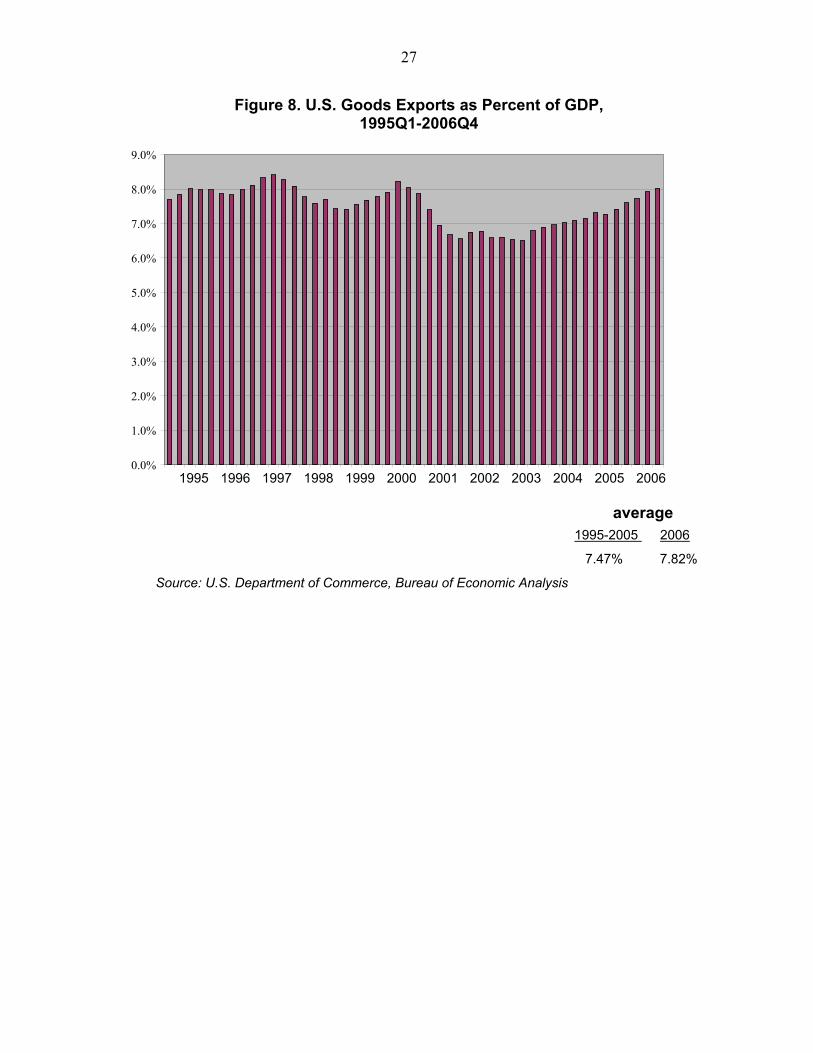
The PPP approach adjusted for the Penn effect also seems to suggest that the dollar was reasonably well aligned in 2006. Recall Figure 3, which is based on cross-section data for 2003. As indicated by the estimated parameter values, the (0,0) point, representing the United States, lies approximately 11.5 percent above the regression line. Accordingly, the adjusted-PPP approach suggests that the dollar was roughly 11.5 percent overvalued in 2003. Since 2003, moreover, the dollar has depreciated; the IMF’s CPI-based real effective exchange rate index declined by 6.5 percent between 2003 and 2006, and the Federal Reserve’s index by about the same amount. Data from the International Comparisons Project are not available for 2006, but it seems reasonable to assume that such data would also show a similar depreciation, implying that the dollar was only about 5 percent above its equilibrium adjusted-PPP level in 2006. Various assessments of the profit and export performance of the U.S tradable goods sector also suggest that the dollar was reasonably well aligned in 2006. Figure 6 plots quarterly data on unit labor costs and prices for the nonfinancial corporate sector. It can be seen that the ratio of unit labor cost to price in 2006 was below its average level over the period 1995-2005, suggesting a healthy profit picture. Much the same impression is provided by Figure 7, which presents data on profit rates in the U.S. manufacturing sector. Although the substantial appreciation of the dollar through 2002 eroded profit rates on durable goods manufactures, which are generally regarded as more tradable than nondurables, by 2006 the profitability of durables manufacturing was back around the levels experienced during the second half of the 1990s. Similarly, while the strong dollar appreciation through 2002 contributed to a decline in goods exports as a share of GDP, by 2006 the exports/GDP ratio was back up to the levels of the late 1990s (Figure 8).

framework calibrated to the United States, see Obstfeld and Rogoff (2005); their framework and perspectives are summarized at the end of this section.

24

Figure 5. Real Effective Exchange Rates: United States, 1980-2006 (CPI-based, 2000=100) 1/

Sources: IMF and Board of Governors of the Federal Reserve System (FRB broad index).

70

80

90

100

110

120

1980 1985 1990 1995 2000 200570

80

90

100

110

120

1/ An increase represents a real appreciation of the U.S. dollar.

average value

1988-1995 1980-2005 2006 IMF 87.23 95.22 92.42

FRB 85.15 91.68 86.71

IMF

FRB

25

Figure 6. Unit Labor Cost and the Implicit Price Deflator for the U.S. Nonfinancial Corporate Sector, 1995 Q1 - 2006 Q4

(Indexes, 1992=100)

90

95

100

105

110

115

120

125

1995 1996 1997 1998 1999 2000 2001 2002 2003 2004 2005 200690

95

100

105

110

115

120

unit labor cost implicit price deflator ratio of unit labor cost to deflator

average value 1995-2005 2006unit labor cost 107.4 115.6 price deflator 109.0 120.2 ratio 98.5 96.2

Source: U.S. Bureau of Labor Statistics

26

Figure 7. After-Tax Profits per Dollar of Sales in U.S. Manufacturing, 1995Q1-2006Q4

(in cents)

-8

-6

-4

-2

0

2

4

6

8

10

12

1995 1996 1997 1998 1999 2000 2001 2002 2003 2004 2005 2006

-8

-6

-4

-2

0

2

4

6

8

10

12

all manufacturing nondurable goods durable goods

average value 1995-2005 2006all manufacturing 5.49 8.30 nondurable goods 6.79 9.78 durable goods 4.33 6.83

Source:U.S. Bureau of the Census, Quarterly Financial Report

27

Figure 8. U.S. Goods Exports as Percent of GDP, 1995Q1-2006Q4

0.0%

1.0%

2.0%

3.0%

4.0%

5.0%

6.0%

7.0%

8.0%

9.0%

1995 1996 1997 1998 1999 2000 2001 2002 2003 2004 2005 2006

Source: U.S. Department of Commerce, Bureau of Economic Analysis

average 1995-2005 2006

7.47% 7.82%

28

By contrast, the macroeconomic balance (MB) framework paints a very different picture. Figure 9 shows the U.S. current account position as a share of GDP. The current account deficit was nearly 5.8 percent of GDP in 2006, and under the assumption that it takes no more than two years to observe the full effects of exchange rate changes on trade volumes, the simple model described in Appendix II suggests that the underlying current account (UCUR) was 5.7 percent of GDP.41 Alternatively, with slower effects on trade volumes—e.g., if only half of the effects of the 13 percent depreciation since 2002 had been realized in 2006--the estimated UCUR deficit would have been 4.3 percent of GDP. These estimated deficits are some 2.3 to 3.7 percent of GDP larger than the average current account deficit over the previous three decades, which might be regarded as a rough approximation to the equilibrium S-I position derived from the regression approach.42 A current account disequilibrium of this magnitude would suggest, according to the simple model described in Appendix II, that the real effective exchange rate of the dollar was overvalued in 2006 by at least 25 percent.

The alternative approach to applying the MB framework is to compare UCUR with the net payment flows required to sustain the prevailing net foreign liability (NFL) position. Figure 10 shows that the U.S. NFL position reached nearly 25 percent of GDP in 2002. It subsequently declined to 17 percent of GDP in 2006, partly because the valuation effects of dollar depreciation outweighed the ongoing effects of large U.S. current account deficits. In the absence of further dollar depreciation, the NFL position would be projected to start increasing again at an annual rate of several percentage points of GDP.

In most cases, countries with positive NFL positions need to generate current account surpluses (i.e., positive net export balances) to stabilize these positions. This is not necessarily the case for the United States, however, which has been able to issue liabilities to nonresidents that offer a much lower average rate of return than it earns on its foreign assets—at least according to official data.

A ballpark estimate of the NFL-stabilizing level of the S-I balance can be derived using the following formula (analogous to those derived in Appendix I)

(S-I)/Y = [(iL-g)/(1+g)](FL/Y) - [(iC-g)/(1+g)](FA/Y) (3)

where

FL/Y = liabilities to foreigners as a ratio to GDP

FA/Y = claims on foreigners as a ratio to GDP

41 As noted in Appendix II, the small difference between UCUR and CUR reflects the fact that the average real exchange rate in 2006 was only 2 percent below its 2004 average while the domestic and foreign output gaps were very small.

42 As noted in Section IV, when equilibrium S-I balances are based on the fitted values of regression models that include country-specific constant terms—as distinct from the preferred approach reported in IMF (2006)—the estimated equilibrium positions tend to closely reflect average current account balances over the historical sample period.

29

Figure 9. US Current Account Balance as a Percent of GDP, 1970-2006 (as defined in national income accounts)

-8

-7

-6

-5

-4

-3

-2

-1

0

1

2

1970 1973 1976 1979 1982 1985 1988 1991 1994 1997 2000 2003 2006

Source: World Economic Outlook

average value 1975-1989 1990-2005 1975-2005 2006 -1.36 -2.50 -1.95 -5.76

standard deviation

1975-1989 1990-2005 1975-2005 1.12 1.70 1.56

30

Figure 10. U.S. Net Foreign Assets as Ratio to GDP, 1980-2006

iL, iC = rates of return on liabilities and claims

g = growth rate of GDP Relevant data and reasonable assumptions for evaluating the formula are:43

FA/Y = 0.83

FL/Y – FA/Y = 0.17 (the estimated NFL/Y ratio for 2006)

43 See Lane and Milesi-Ferretti (2005, pp. 19-20 and 28); the FA/Y ratio assumes that most of the decline in NFL/Y between 2004 and 2006 reflected a rise in FA/Y. It may be noted that equity holdings account for roughly 60 percent of U.S. gross claims on nonresidents and 40 percent of U.S. gross liabilities to nonresidents (with the value of US gross equity claims increasing more than the value of its gross equity liabilities as stock prices rose at home and abroad between 2004 and 2006), and that iL and iC are constructed as sums of investment income and capital gains divided by the relevant stocks of assets or liabilities. See also Gros (2006), who suggests that the large difference between iC and iL in the official data is misleading because foreign direct investors in the United States have incentives to escape U.S. tax liabilities by shifting reported profits outside the United States while U.S. firms do not face higher tax liabilities if they report foreign profits to the U.S. authorities.

-0.28

-0.20

-0.12

-0.04

0.04

0.12

1980 1982 1984 1986 1988 1990 1992 1994 1996 1998 2000 2002 2004 2006

-0.28

-0.20

-0.12

-0.04

0.04

0.12

Source: Research Department, IMF

31

iL = .04 (the average over the 20 years through 2004)

iC - iL = .03 (the average over 1990-2004)

g = .03

Together, the above formula and numbers suggest that the level of the S-I balance required to stabilize the NFL/Y ratio in 2006 was a deficit of roughly 2.3 percent of GDP—some 2 to 3.4 percentage points smaller than the estimates of the UCUR deficit. Thus, this approach to applying the macroeconomic balance framework suggests that the dollar was overvalued in 2006 by at least 20 percent.

It may be noted that the impressions conveyed by the macroeconomic balance framework are somewhat analogous to perspectives provided by Obstfeld and Rogoff (2005), who develop an analysis based on a small general equilibrium model that distinguishes between tradable and nontradable goods. The Obstfeld-Rogoff (OR) approach does not take a stand on the equilibrium levels of either the S-I balance or the real exchange rate. Instead, it focuses on various plausible types of “shocks” to domestic or foreign saving or productivity that might play a role in reducing the U.S. current account deficit. Each of these shocks has effects, inter alia, on both the current account and the real exchange rate of the dollar, and the OR model provides quantitative perspectives on how much dollar depreciation might accompany a reduction of the U.S. current account deficit under the various shocks. Writing in November 2005, OR concluded that: “Notwithstanding ... [various] qualifications, and given the depreciation that has already occurred in the last couple of years, it still seems quite conservative to suppose that the trade weighted dollar needs to depreciate at least another 20-25% as the current account rebalances.”

IX. WHICH ASSESSMENT METHODOLOGIES DESERVE THE MOST WEIGHT?

What should be concluded from the different assessments of the U.S. dollar? Should the suggestions of the macroeconomic balance approach (along with the parallel OR focus on current account adjustment) be dismissed because three other approaches suggest that the dollar was reasonably well-aligned in 2006? Would our judgment be the same if the macroeconomic balance approach suggested that the dollar was well aligned but the purchasing power parity approaches (adjusted and unadjusted) suggested otherwise? Would we feel more confident or less confident in our judgment if the macroeconomic balance assessments were ambiguous but an assessment based on an estimated exchange rate equation suggested that the dollar was considerably overvalued?

In general, the criteria that are most appealing for assessing the exchange rate of an individual country may not be the most appealing ones when selecting methodologies for multilateral assessment exercises. In the former case, the primary objective is to judge whether the prevailing level of the exchange rate is likely to lead to major problems for the individual country, such as a currency crisis or economic stagnation. Multilateral assessment exercises also seek to identify prospective difficulties for individual countries, but a broader objective is to assess whether countries’ policies—and particularly the policies of large

32

countries—are consistent with a code of conduct for contributing to external stability and the smooth functioning of the international monetary system.

This section focuses on criteria that seem relevant to the choice of methodologies for individual country assessments.44 It starts by posing the questions: Which approaches for assessing misalignment draw support from theoretical models for predicting currency crises in emerging market countries? And which approaches draw support from what we think we know about factors that are important for economic growth? It then sifts the alternatives in a different way by asking: Which approaches point to situations that policymakers and the general public would be most likely to regard as serious problems and persuasive rationales for either exchange rate realignment or other policy adjustments?

Currency crisis models address the types of factors that can give rise to speculative attacks on a fixed exchange rate regime. The academic literature is often divided into two generations of models. First generation models, launched from seminal contributions by Krugman (1979) and Flood and Garber (1984), focus on a country’s holdings of foreign exchange reserves. These models treat macroeconomic policies as exogenous and generally link currency crises to the inflationary consequences of either large fiscal deficits or rapid monetary growth. Rapid inflation (relative to trading partners) with a fixed nominal exchange rate leads to real appreciation, resulting in growing current account deficits that drain the country’s foreign exchange reserves. Market participants anticipate that the country will run out of reserves and be forced to devalue; and with one-sided forward-looking expectations, the speculative attack may come well before the country runs out of reserves.

In contrast to first generation models—where currency crises arise because market participants anticipate that countries will lose their ability or financial capacity to defend a fixed exchange rate—second generation models emphasize that speculative attacks can also occur when there are doubts about a country’s willingness or political capacity to defend its currency. The latter models, widely associated with an early contribution by Obstfeld (1994), were inspired by the 1992 speculative attacks on the European Exchange Rate Mechanism (ERM). The build-up to that crisis started with the unification of Germany in 1990, which had major fiscal consequences that led the Bundesbank to raise interest rates. The rise in German interest rates, in combination with obligations to defend fixed exchange rates against the Deutschemark, forced parallel interest rate increases in other ERM countries. This contributed to high unemployment rates in Europe, and in the run-up to the 1992 crisis the tight monetary policies required to sustain the ERM were losing public support. Thus, in a June 1992 referendum, Denmark voted against participating in the next step toward a European common currency area; and in August, public opinion polls began to suggest that a French referendum scheduled for late September might also generate a “no” vote. Such “news” led to doubts not only about the fate of plans for the common currency area, but also about the viability of existing exchange rate parities among the ERM currencies. In particular, it contributed to a growing sense that—despite having access to the financing

44 It does not address the choice of methodologies for multilateral assessment exercises, which has received considerable attention in IMF (2006).

33

facilities of the ERM and, hence, having the ability to mobilize very large volumes of foreign exchange in defense of their currencies—the governments of some ERM countries might succumb to political pressures. This translated into growing expectations that some countries would either devalue their currencies within the ERM or withdraw from the ERM, adopt more stimulative monetary policies, and let their currencies depreciate. Consequently, prudential market participants became more concerned to cover long positions in currencies that were vulnerable to depreciation (but would not appreciate), speculators saw the potential to profit from opening short positions in those currencies, and the process snowballed as rising market tensions made prudent investors increasingly concerned about the need for defensive cover and speculators increasingly optimistic about the prospect for profit.

Currency crisis models took on new dimensions following the Asian crises in 1997-98. In particular, models of currency crises began to reflect economists’ growing awareness of the vulnerabilities associated with mismatches between the currency compositions of a country’s financial assets and liabilities, and between the maturities of those assets and liabilities. Although this led some economists to refer to a third generation of models, the main contribution of the new models was to illustrate that balance sheet mismatches add to the vulnerabilities that macroeconomic imbalances create. The new models did not alter the perspective that currency crises are triggered by doubts about either a country’s ability (financial capacity) to sustain a fixed exchange rate or its willingness (political capacity) to do so.

The currency crisis literature provides one source of guidance when judging the relative merits of different approaches for assessing equilibrium exchange rates. To the extent that the large welfare losses associated with currency crises are regarded as the main potential costs of overvaluation in advanced and emerging market countries, it would seem appropriate to pay particular attention to assessment methodologies that focus on a country’s ability or willingness to resist a depreciation of its currency.45 This suggests that relatively large weights should be given to the external sustainability variant of macroeconomic balance assessments, and to assessments of the health of the tradable goods sector. The macroeconomic balance framework, when used to assess whether a country’s underlying current account balance can sustain its prevailing net foreign liability position, is directly focused on the country’s ability (financial capacity) to sustain the prevailing exchange rate. And while none of the methodologies focuses directly on the willingness (political capacity) of countries to sustain their prevailing exchange rates, history suggests that political pressures for import protection and exchange rate market intervention tend to develop and intensify—and can trigger speculative pressures on exchange rates—when the tradable goods sector loses competitiveness.

45 The literature on currency crises arising from prolonged and substantial overvaluations does not have a counterpart literature on catastrophic events that arise from prolonged and substantial undervaluations. This suggests that there may be asymmetry between the potential costs of undervaluation and overvaluation, and that countries’ abilities and willingness to resist appreciation may be greater than their capacities to resist depreciation.

34

The same two approaches seem particularly relevant for low income countries. External debt sustainability is one of the prerequisites for sustainable growth, and few (if any) countries have been able to achieve sustained growth without outward-looking policies and a healthy tradable goods sector.46

Another feature of the macroeconomic balance framework and assessments of tradable goods competitiveness is that assessments of overvaluation based on those approaches point directly to developments that policymakers and the public can easily relate to as problematic for macroeconomic performance and justification for either exchange rate realignment or other policy changes. In particular, the concepts of growing external indebtedness and an unhealthy tradable goods sector do not require much explanation, and it is also relatively easy to convey a sense that failure to address such situations is likely to have adverse consequences. By contrast, it is much harder to convey an understanding of regression residuals and simulations of general equilibrium models. This makes it relatively difficult to convince policymakers and the general public that there is an underlying problem when the assessment of overvaluation comes from an estimated exchange rate equation or the application of a general equilibrium model.

These views are intended as a guide for prioritizing approaches to exchange rate assessments for countries individually.47 Top priority has been given to the methodologies that seem best suited for identifying when countries are ripe for currency crises or growth failures—two dire consequences of substantial and prolonged overvaluation. While the consequences of substantial undervaluation may not be as severe as those of overvaluation, they can also be detrimental to macroeconomic prospects, and the same two methodologies are useful for raising warning flags in such cases. Excessive profitability of the tradable goods sector that is not likely to be sustained over the medium run can lead to overinvestment in that sector and underinvestment in nontradables. Similarly, large and prolonged current account surpluses can signal a misallocation of resources from a medium-run perspective, with overinvestment in producing goods for export and underinvestment in producing for the domestic market. For large countries, excessive tradable goods profitability, and/or large and prolonged current account surpluses, can also be a signal that domestic policies are contributing to macroeconomic difficulties in other countries and thereby posing a threat to external stability.

X. CONCLUSIONS

This paper has described six different approaches for estimating equilibrium exchange rates and has applied four of them to data for the United States. It has emphasized that each

46 Johnson, Ostry, and Subramanian (2007) provide recent support for the view that success in sustaining growth depends importantly on the ability of the manufacturing sector to compete internationally.

47 Such prioritization is not meant to discourage policymaking institutions from striving to include carefully specified general equilibrium models and estimated exchange rate equations in their toolkits. Indeed, many economists are uncomfortable with policy conclusions that are not supported by either a carefully specified general equilibrium model or state-of-the-art econometric analysis.

35

methodology involves conceptual simplifications and/or imprecise estimates of key parameters, and it has illustrated that different methodologies sometimes generate markedly different quantitative estimates of equilibrium exchange rates. These facts suggest that the assessment of equilibrium exchange rates requires considerable judgment, and that policymakers, ideally, should inform their judgments through the application of several different methodologies.

Although the mandates of some policy institutions (the IMF in particular) make it important for them to invest considerable resources in developing different methodologies for exchange rate assessment—with emphasis on global consistency and attention to the different types of perspectives that different methodologies provide—other interested parties (including national policymaking agencies) may not be in a position to devote extensive resources to assessment exercises. How should such parties prioritize the different approaches? It can be argued, in principle, that judgments about the relative merits of the different approaches should be based on tests of their abilities to explain the equilibrating tendencies of exchange rates out-of-sample, after allowing for unexpected changes in exogenous variables. In practice, however, such tests would be difficult to conduct. Accordingly, this paper has suggested other criteria that may be appealing for prioritizing among methodologies, starting from the presumption that a major part of the rationale for estimating equilibrium exchange rates—particularly in applications that focus on countries individually—is to judge whether prevailing exchange rates are likely to lead to serious macroeconomic difficulties, other things equal.

In suggesting ways to prioritize, the paper has noted that relevant perspectives can be found in the currency crisis literature, in accepted wisdom on the factors contributing to economic growth, and by focusing on the challenge of being persuasive to policymakers and the general public. From those perspectives, the paper has argued that:

● Insofar as currency crises can give rise to very large welfare losses, emphasis should be given to methodologies that address a country’s ability (financial capacity) or willingness (political capacity) to sustain the level of its exchange rate and resist speculative attacks on its currency.

● This suggests that relatively large weights should be placed on the external sustainability variant of the macroeconomic balance approach, which bears on the financial capacity to defend against speculative attacks, and assessments of the competitiveness of the tradable goods sector, which bear on the political capacity.

● These two approaches for assessing exchange rates also focus directly on factors that bear importantly on the outlook for growth in low income countries.

● Furthermore, these approaches have the merit that policymakers and the general public can readily relate to the fact that large and growing external indebtedness and unhealthy tradable goods sectors generally have undesirable consequences. Policymakers are not likely to be easily convinced that the exchange rate is contributing to serious problems if the assessment of substantial overvaluation is based simply on an estimated exchange rate equation or simulation of a general equilibrium model.

36

The case for the two approaches favored here needs to be qualified by emphasizing that it would be dangerous to use any approach mechanically. As noted earlier, for example, the macroeconomic balance approach (including the external sustainability variant) may not be very helpful for countries that have bright prospects for economic growth and are attracting large volumes of capital inflows mirrored by large current account deficits. In such cases, an assessment of whether the prevailing level of the exchange rate is likely to lead to serious macroeconomic difficulties, ceteris paribus, requires considerable judgment that takes into account, among other things, the degree to which the capital inflows are supporting productive investments and a prospective unwinding of current account deficits. The arguments in favor of two specific approaches should not be interpreted as criticism of other methodologies. Policymaking institutions may find it useful to have more than two assessment methodologies in the toolkits they rely upon for informing their judgments about equilibrium exchange rates. This is particularly the case for institutions engaging in multilateral assessment exercises.48

As a final point, it should be noted—as many policymakers have emphasized--that there is no general answer to the question of what to do when an exchange rate is judged to differ substantially from its equilibrium level. Exchange rate adjustment is not always the best answer or the only part of the answer. Policy advice on the best course of action—whether viewed from a global perspective or the perspective of an individual country’s ultimate targets—needs to be framed in the context of an overall assessment of the prevailing macroeconomic situation and the risks to the macroeconomic outlook.

48 It may be noted that the macroeconomic balance approach has been a centerpiece of the IMF’s arsenal for some time, and that the external sustainability variant has recently received renewed emphasis; see Isard and Faruqee, eds. (1998) and IMF (2006). By contrast, assessments of the health of the tradable goods sector can be conducted on a country-by-country basis but would be constrained by—and in that sense are probably not as conducive to—multilateral exercises. Ideally, assesssments of the latter type should focus on a range of indicators of international competitiveness, and the data available for such assessments tend to differ across countries and are not always strictly comparable internationally.

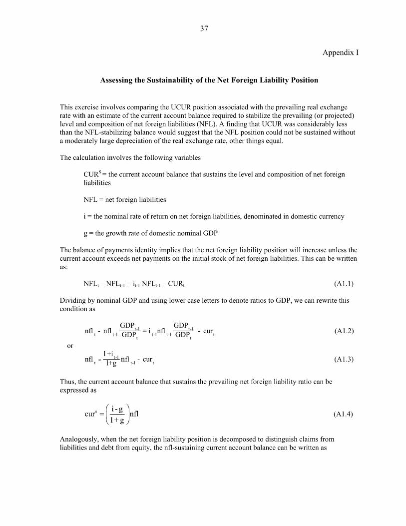
37

Appendix I

Assessing the Sustainability of the Net Foreign Liability Position

This exercise involves comparing the UCUR position associated with the prevailing real exchange rate with an estimate of the current account balance required to stabilize the prevailing (or projected) level and composition of net foreign liabilities (NFL). A finding that UCUR was considerably less than the NFL-stabilizing balance would suggest that the NFL position could not be sustained without a moderately large depreciation of the real exchange rate, other things equal. The calculation involves the following variables CURS = the current account balance that sustains the level and composition of net foreign

liabilities NFL = net foreign liabilities i = the nominal rate of return on net foreign liabilities, denominated in domestic currency g = the growth rate of domestic nominal GDP The balance of payments identity implies that the net foreign liability position will increase unless the current account exceeds net payments on the initial stock of net foreign liabilities. This can be written as: NFLt – NFLt-1 = it-1 NFLt-1 – CURt (A1.1) Dividing by nominal GDP and using lower case letters to denote ratios to GDP, we can rewrite this condition as

t-1 t-1t t-1 t-1 t-1 t

t t

GDP GDPnfl - nfl = i nfl - curGDP GDP (A1.2)

or

t-1=t t-1 t

l +infl fl - curl+g n (A1.3)

Thus, the current account balance that sustains the prevailing net foreign liability ratio can be expressed as

s i - gcur nfl1+ g⎛ ⎞

= ⎜ ⎟⎝ ⎠

(A1.4)

Analogously, when the net foreign liability position is decomposed to distinguish claims from liabilities and debt from equity, the nfl-sustaining current account balance can be written as

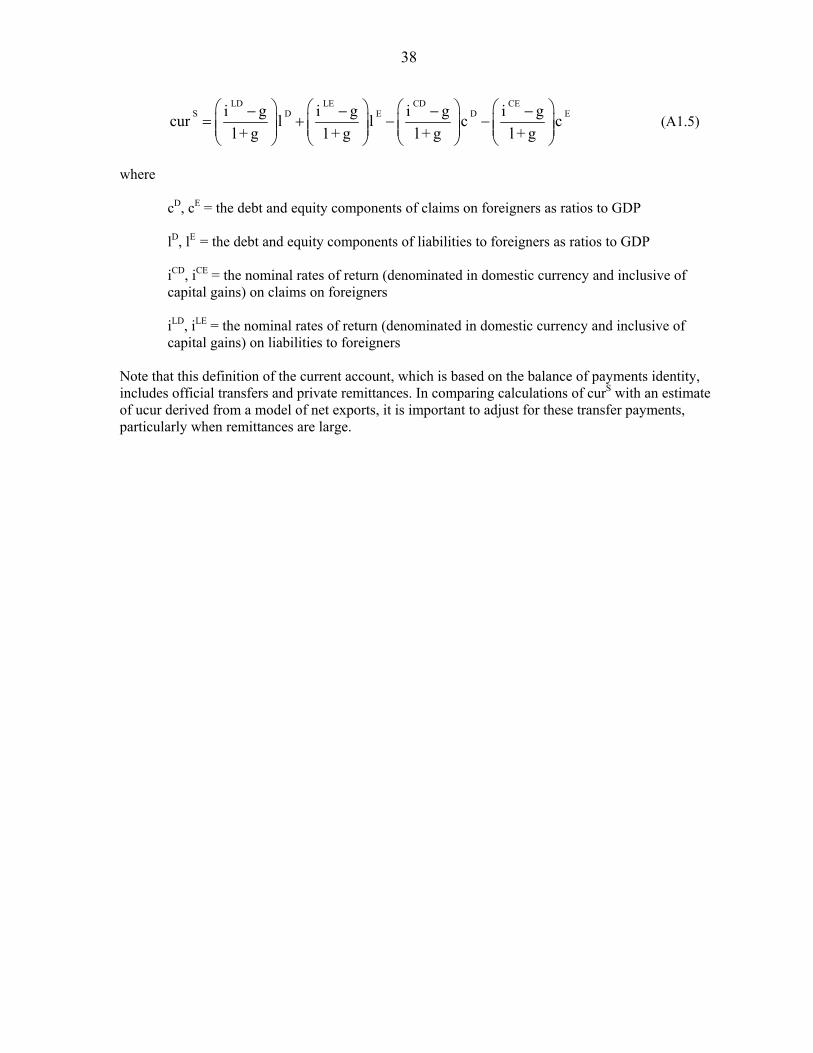
38

LD LE CD CE

S D E D Ei g i g i g i gcur l l c cl + g 1+ g l + g l + g

⎛ ⎞ ⎛ ⎞ ⎛ ⎞ ⎛ ⎞− − − −= + − −⎜ ⎟ ⎜ ⎟ ⎜ ⎟ ⎜ ⎟⎜ ⎟ ⎜ ⎟ ⎜ ⎟ ⎜ ⎟⎝ ⎠ ⎝ ⎠ ⎝ ⎠ ⎝ ⎠

(A1.5)

where cD, cE = the debt and equity components of claims on foreigners as ratios to GDP lD, lE = the debt and equity components of liabilities to foreigners as ratios to GDP iCD, iCE = the nominal rates of return (denominated in domestic currency and inclusive of

capital gains) on claims on foreigners

iLD, iLE = the nominal rates of return (denominated in domestic currency and inclusive of capital gains) on liabilities to foreigners

Note that this definition of the current account, which is based on the balance of payments identity, includes official transfers and private remittances. In comparing calculations of curS with an estimate of ucur derived from a model of net exports, it is important to adjust for these transfer payments, particularly when remittances are large.

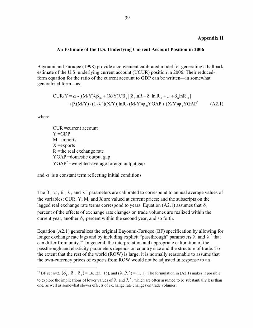
39

Appendix II

An Estimate of the U.S. Underlying Current Account Position in 2006

Bayoumi and Faruqee (1998) provide a convenient calibrated model for generating a ballpark estimate of the U.S. underlying current account (UCUR) position in 2006. Their reduced-form equation for the ratio of the current account to GDP can be written—in somewhat generalized form—as: m x o 1 -1 n -nCUR/Y = -[(M/Y) (X/Y) ][ lnR ln R ... lnR ]α ∗λβ + λ β δ + δ + + δ *

m x[ Y) - (1- )(X/Y)]lnR - (M/Y) YGAP (X/Y) YGAP∗+ λ(Μ/ λ ψ + ψ (A2.1) where CUR =current account Y =GDP M =imports X =exports R =the real exchange rate YGAP =domestic output gap *YGAP =weighted-average foreign output gap and α is a constant term reflecting initial conditions The β , ψ , δ , λ , and λ * parameters are calibrated to correspond to annual average values of the variables; CUR, Y, M, and X are valued at current prices; and the subscripts on the lagged real exchange rate terms correspond to years. Equation (A2.1) assumes that oδ percent of the effects of exchange rate changes on trade volumes are realized within the current year, another 1δ percent within the second year, and so forth. Equation (A2.1) generalizes the original Bayoumi-Faruqee (BF) specification by allowing for longer exchange rate lags and by including explicit “passthrough” parameters λ and λ * that can differ from unity.49 In general, the interpretation and appropriate calibration of the passthrough and elasticity parameters depends on country size and the structure of trade. To the extent that the rest of the world (ROW) is large, it is normally reasonable to assume that the own-currency prices of exports from ROW would not be adjusted in response to an 49 BF set n=2, o(δ , 1δ , 2 )δ = (.6, .25, .15), and (λ ,λ * ) = (1, 1). The formulation in (A2.1) makes it possible

to explore the implications of lower values of λ and λ * , which are often assumed to be substantially less than one, as well as somewhat slower effects of exchange rate changes on trade volumes.

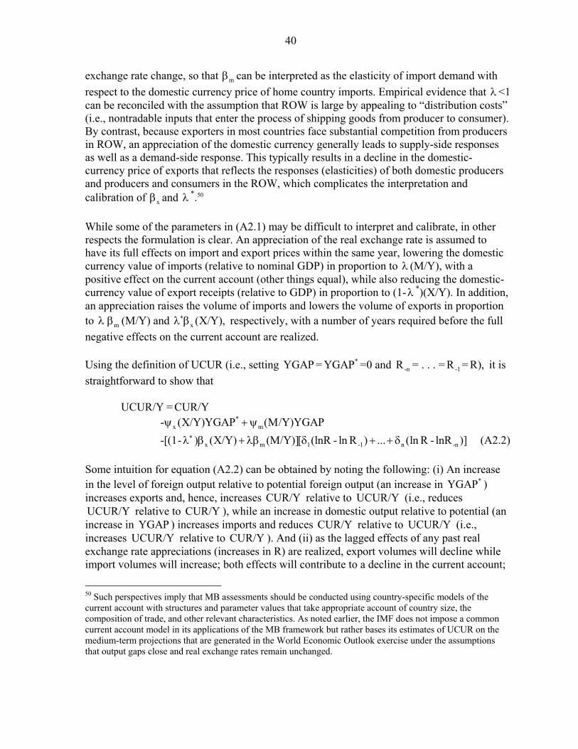
40

exchange rate change, so that mβ can be interpreted as the elasticity of import demand with respect to the domestic currency price of home country imports. Empirical evidence that λ<1 can be reconciled with the assumption that ROW is large by appealing to “distribution costs” (i.e., nontradable inputs that enter the process of shipping goods from producer to consumer). By contrast, because exporters in most countries face substantial competition from producers in ROW, an appreciation of the domestic currency generally leads to supply-side responses as well as a demand-side response. This typically results in a decline in the domestic-currency price of exports that reflects the responses (elasticities) of both domestic producers and producers and consumers in the ROW, which complicates the interpretation and calibration of xβ and λ *.50 While some of the parameters in (A2.1) may be difficult to interpret and calibrate, in other respects the formulation is clear. An appreciation of the real exchange rate is assumed to have its full effects on import and export prices within the same year, lowering the domestic currency value of imports (relative to nominal GDP) in proportion to λ (M/Y), with a positive effect on the current account (other things equal), while also reducing the domestic-currency value of export receipts (relative to GDP) in proportion to (1-λ *)(X/Y). In addition, an appreciation raises the volume of imports and lowers the volume of exports in proportion to λ mβ (M/Y) and x (X/Y), ∗λ β respectively, with a number of years required before the full negative effects on the current account are realized. Using the definition of UCUR (i.e., setting YGAP = *YGAP =0 and -nR = . . . = -1R = R), it is straightforward to show that UCUR/Y = CUR/Y *

x m- (X/Y)YGAP Y)YGAPψ +ψ (Μ/ x m 1 -1 n -n-[(1- (X/Y) (M/Y)][ (lnR - ln R ) ... (ln R - lnR )]∗λ )β + λβ δ + + δ (A2.2) Some intuition for equation (A2.2) can be obtained by noting the following: (i) An increase in the level of foreign output relative to potential foreign output (an increase in *YGAP ) increases exports and, hence, increases CUR/Y relative to UCUR/Y (i.e., reduces UCUR/Y relative to CUR/Y ), while an increase in domestic output relative to potential (an increase in YGAP ) increases imports and reduces CUR/Y relative to UCUR/Y (i.e., increases UCUR/Y relative to CUR/Y ). And (ii) as the lagged effects of any past real exchange rate appreciations (increases in R) are realized, export volumes will decline while import volumes will increase; both effects will contribute to a decline in the current account;

50 Such perspectives imply that MB assessments should be conducted using country-specific models of the current account with structures and parameter values that take appropriate account of country size, the composition of trade, and other relevant characteristics. As noted earlier, the IMF does not impose a common current account model in its applications of the MB framework but rather bases its estimates of UCUR on the medium-term projections that are generated in the World Economic Outlook exercise under the assumptions that output gaps close and real exchange rates remain unchanged.

41

so the extent to which UCUR/Y is lower than CUR/Y is positively related to both the initial level of exports and the initial level of imports, other things equal. The model of CUR described by equation (A2.1) implies the following relationship between changes in R and changes in UCUR : m x(UCUR/Y) = [ (M/Y) - (1- )(X/Y)] lnR -[ (M/Y) + (X/Y)] lnR∗ ∗Δ λ λ Δ λβ λ β Δ m x- )(M/Y) + ( (1- ) 1)(X/Y)] lnR∗= [λ(1 β λ β − Δ (A2.3) The first term in the top line captures the response of UCUR/Y to the downward effects of exchange rate appreciation on import and export prices, while the remainder of the top line captures the effects that are channeled through changes in import and export volumes. This equation can be inverted to provide an expression for the change in lnR (or, approximately, the percentage change in R) that is required to adjust UCUR/Y from its prevailing level to the equilibrium (S-I)/Y position: lnR = {(S- I)/Y - UCUR/Y}σΔ (A2.4) where m xl )(M/Y) + ( ) 1)(X/Y)]σ ∗= /[λ(1−β λ (1−β − (A2.5) Note that the value of σ is sensitive to the scale of imports and exports relative to GDP (the degree of openness), the “passthrough” effects of exchange rate changes on import and export prices, and the exchange rate elasticities of import and export volumes. The next step is to generate numerical estimates of UCUR/Y. Relevant values of the variables (for 2006) are51 CUR/Y = -.0576 X/Y = .1107 M/Y = .1683 *YGAP = .0007 YGAP = -.0018 R = 92.42 -1R = 92.75 -2R = 94.12 ln R = 4.526 -1ln R = 4.530

51 YGAP and *YGAP are constructed as logarithms of observed output divided by logarithms of potential output. The values for 2006 are IMF staff estimates.

42

-2lnR = 4.545 and the parameter values suggested by Bayoumi and Faruqee are xβ = 0.71 mβ = 0.92 xψ = 1.50 mψ = 1.50 0δ = 0.6 1δ = 0.25 2δ = 0.15 λ= 1 λ * = 1 Under these variable values and parameters, equation (A2.2) implies UCUR/Y = -.0573, which is not much different than CUR/Y. This is not surprising, given that the dollar depreciated by only 2 percent between 2004 and 2006 (based on annual average exchange rates) and that the 2006 output gaps were small. Moreover, given the small amount of depreciation, the calculated value of UCUR/Y is not very sensitive to the calibrations of λ and λ *. Note, however, that slower effects of exchange rate changes on trade volumes would lower the calculated UCUR deficit. For example, if only half of the effects on trade volumes of the dollar’s 13 percent depreciation since 2002 had been realized in 2006, the implied value of UCUR/Y would be approximately -.043. The final step is to calculate the value of σ , which is relevant for estimating how much the real exchange rate would need to depreciate, other things equal, to achieve a given improvement in UCUR/Y. Under the variable and parameter values listed above, (A2.5) implies σ = -15.4. Unlike the estimates of UCUR, this calculation is moderately sensitive to the assumed degrees of passthrough into import and export prices. Thus, if λ was lowered from 1.0 to 0.4, consistent with some estimates for the United States,52 the calculated value of σ would be -13.7; and if λ and λ * were both lowered to 0.4, the calculated value of σ would be -10.8.

52 See Campa and Goldberg (2006).

43

REFERENCES Artus, Jacques R., 1978, “Methods of Assessing the Long-Run Equilibrium Value of an

Exchange Rate,” Journal of International Economics, Vol. 8, pp. 277-99. _______ , and Malcolm D. Knight, 1984, Issues in the Assessment of Exchange Rates of the

Industrial Countries, Occasional Paper No. 29 (Washington: International Monetary Fund).

Asea, Patrick K., and Enrique G. Mendoza, 1994, “The Balassa-Samuelson Model: A

General-Equilibrium Appraisal,” Review of International Economics, Vol. 2 (October), pp. 244-67.

Balassa, Bela, 1964, “The Purchasing-Power-Parity Doctrine: A Reappraisal,” Journal of

Political Economy, Vol. 72, pp. 584-96. Bayoumi, Tamim, and Hamid Faruqee, 1998, “A Calibrated Model of the Underlying

Current Account,” in Exchange Rate Assessment: Extensions of the Macroeconomic Balance Approach, Occasional Paper No. 167, ed. By Peter Isard and Hamid Faruqee (Washington: International Monetary Fund).

Campa, José Manuel, and Linda Goldberg, 2006, “Pass Through of Exchange Rates to

Consumption Prices: What Has Changed and Why?”, NBER Working Paper 12547. Canzoneri, Matthew, Robert Cumby, and Behzad Diba, 1999, “Relative Labor Productivity

and the Real Exchange Rate in the Long Run: Evidence for a Panel of OECD Countries,” Journal of International Economics, Vol. 47, pp. 245-66.

Cassel, Gustav, 1918, “Abnormal Deviations in International Exchanges,” Economic

Journal 28, pp. 413-15. _______ , 1922, Money and Foreign Exchange After 1914 (New York: Constable & Co.). Chen, Yu-chin, and Kenneth Rogoff, 2003, “Commodity Currencies,” Journal of

Internationa Economics, Vol. 60, pp. 133-60. Chinn, Menzie, and Eswar Prasad, 2003, “Medium-Term Determinants of Current Accounts

in Industrial and Developing Countries: An Empirical Exploration,” Journal of International Economics, Vol. 59, No. 1, pp. 47-76.

Choudhri, Ehsan, and Mohsin Khan, 2005, “Real Exchange Rates in Developing Countries:

Are Balassa-Samuelson Effects Present?” Staff Papers, Vol. 52, No. 3, pp. 387-409 (Washington: International Monetary Fund).

44

De Broeck, Mark, and Torsten Slok, 2001, “Interpreting Real Exchange Rate Movements in Transition Countries,” IMF Working Paper WP/01/56.

Debelle, Guy, and Hamid Faruqee, 1996, “What Determines the Current Account? A Cross-

Sectional and Panel Approach,” IMF Working Paper No. 96/58. De Gregorio, José, Alberto Giovannini, and Thomas H. Krueger, 1994, “The Behavior of

Nontradable-Goods Prices in Europe: Evidence and Interpretation,” Review of International Economics, Vol. 2 (October), pp. 284-305.

De Gregorio, José, Alberto Giovannini, and Holger C. Wolf, 1994, “International Evidence

on Tradables and Nontradables Inflation,” European Economic Review, Vol. 38 (June), pp. 1225-44.

Einzig, Paul, 1970, The History of Foreign Exchange (London: Macmillan). Engel, Charles, Nelson Mark, and Kenneth West, 2007, “Exchange Rate Models Are Not as

Bad as You Think,” in NBER Macroeconomics Annual 2007, ed. by Daron Acemoglu, Kenneth Rogoff, and Michael Woodford, forthcoming.

Engel, Robert F., and C.W.J. Granger, 1987, “Co-integration and Error Correction:

Representation, Estimation, and Testing,” Econometrica, Vol. 55 (March), pp. 251-76.

Evans, Martin, and Richard Lyons, 2002, “Order Flow and Exchange Rate Dynamics,”

Journal of Political Economy, Vol. 110, pp. 170-80. _______ , 2005, “Meese-Rogoff Redux: Micro-Based Exchange-Rate Forecasting,”

American Economic Review, Vol. 95, pp. 405-14. Faruqee, Hamid, 1995, “Long-Run Determinants of the Real Exchange Rate: A Stock-Flow

Perspective,” Staff Papers, Vol. 42, No. 1, pp. 80-107 (Washington: International Monetary Fund).

_______ , 1998, “Methodology for Calculating Equilibrium Exchange Rates and Question of

Global Consistency,” in Exchange Rate Assessment: Extensions of the Macroeconomic Balance Approach, Occasional Paper No. 167, ed. By Peter Isard and Hamid Faruqee (Washington: International Monetary Fund).

_______ , 2004, “Global Rebalancing of Current Accounts: A Euro-Area Perspective,” in

International Monetary Fund, Euro Area Policies-Selected Issues (available at www.imf.org).

Faruqee, Hamid, Douglas Laxton, Dirk Muir, and Paolo Pesenti, 2005, “Smooth Landing or

Crash? Model-Based Scenarios of Global Current Account Rebalancing,” NBER Working Paper 11583.

45

Flood, Robert P., and Peter M. Garber, 1984, “Collapsing Exchange Regimes: Some Linear

Examples,” Journal of International Economics 17, pp. 1-13. Flood, Robert P., and Andrew K. Rose, 1999, “Understanding Exchange Rate Volatility

Without the Contrivance of Macroeconomics,” Economic Journal, Vol. 109, No. 459 (November), pp. F660-72.

Flood, Robert P., and Mark P. Taylor, 1996, “Exchange Rate Economics: What’s Wrong

with the Conventional Macro Approach?” in The Microstructure of Foreign Exchange Markets, ed. By Jeffrey A. Frankel, Giampaolo Galli, and Alberto Giovannini (Chicago: University of Chicago Press).

Frankel, Jeffrey, 2006, “The Balassa-Samuelson Relationship and the Renminbi,” Working

Paper (available at ksghome.harvard.edu/~jfrankel). Frankel, Jeffrey A., and Andrew K. Rose, 1995, “A Survey of Empirical Research on

Nominal Exchange Rates,” in Handbook of International Economics, ed. by Gene Grossman and Kenneth Rogoff, Vol. 3 (Amsterdam: North-Holland).

Froot, Kenneth A., and Kenneth Rogoff, 1995, “Perspectives on PPP and Long-Run Real

Exchange Rates,” in Handbook of International Economics, ed. By Gene Grossman and Kenneth Rogoff, Vol. 3 (Amsterdam: North-Holland).

Gilbert, Milton, and Irving B. Kravis, 1954, An International Comparison of National

Products and the Purchasing Power of Currencies: A Study of the United States, the United Kingdom, France, Germany, and Italy (Paris: Organization for European Economic Cooperation).

Granger, C.W.J., 1981, “Some Properties of Time Series Data and Their Use in Econometric

Model Specification,” Journal of Econometrics, Vol. 16 (No. 1), pp. 121-30. Grice-Hutchinson, Marjorie, 1952, The School of Salamanca (Oxford: Clarendon Press). Gros, Daniel, 2006, “Foreign Investment in the US (II): Being Taken to the Cleaners?”

Center for European Policy Studies, CEPS Working Document No. 243. Harrod, Roy F., 1939, International Economics (London: Nisbet & Co. Ltd.). International Monetary Fund, 2006, “Methodology for CGER Exchange Rate Assessments,”

(available at www.imf.org). Isard, Peter, 1995, Exchange Rate Economics (Cambridge: Cambridge University Press).

46

Isard, Peter, and Hamid Faruqee, eds., 1998, Exchange Rate Assessment: Extensions of the Macroeconomic Balance Approach, Occasional Paper No. 167 (Washington: International Monetary Fund).

Isard, Peter, Hamid Faruqee, Russell Kincaid, and Martin Fetherston, 2001, Methodology for

Current Account and Exchange Rate Assessment, Occasional Paper No. 209 (Washington: International Monetary Fund).

Isard, Peter, and Steven Symansky, 1996, “Long-Run Movements in Real Exchange Rates,”

in Exchange Rate Movements and Their Impact on Trade and Investment in the APEC Region, Occasional Paper No. 145, ed. By Takatoshi Ito and others (Washington: International Monetary Fund).

Johnson, Simon, Jonathan Ostry, and Arvind Subramanian, 2007, “The Prospects for

Sustained Growth in Africa: Benchmarking the Constraints,” NBER Working Paper 13120.

Keynes, John Maynard, 1925, “The Economic Consequences of Mr. Churchill,” Essays in

Persuasion (London: Hogarth Press). Kravis, Irving B., Alan Heston, and Robert Summers, 1982, World Product and Income:

International Comparisons of Real Gross Product (Baltimore: Johns Hopkins University Press).

Krugman, Paul, 1979, “A Model of Balance-of-Payments Crises,” Journal of Money, Credit

and Banking 11, pp. 311-25. _______ , 1993, “Recent Thinking About Exchange Rate Determination and Policy,” in

Blundell-Wignall (ed.), pp. 6-21. Lane, Philip and Gian Maria Milesi-Ferretti, 2005, “A Global Perspective on External

Positions,” IMF Working Paper 05/161. Lee, Jaewoo and Man-Keung Tang, 2007, “Does Productivity Growth Appreciate the Real

Exchange Rate?,” Review of International Economics, Vol. 15, pp. 164-87. Lipschitz, Leslie and Donogh McDonald, 1992, “Real Exchange Rates and Competitiveness:

A Clarification of Concepts and Some Measurement for Europe,” Empirica-Austrian Economic Papers, Vol. 19, pp. 37-69.

Meade, James E., 1951, The Theory of International Economic Policy Volume One: the

Balance of Payments (London: Oxford University Press). Meese, Richard A., and Kenneth Rogoff, 1983a, “Empirical Exchange Rate Models of the

Seventies: Do They Fit Out of Sample?” Journal of International Economics, Vol. 14, pp. 3-24.

47

_______ , and _______ , 1983b, “The Out-of-Sample Failure of Empirical Exchange Rate

Models: Sampling Error or Misspecification?” in Exchange Rates and International Macroeconomics, ed. by Jacob Frenkel, pp. 67-112 (Chicago: Chicago University Press).

Metzler, Loyd A., 1951, “Wealth, Saving, and the Rate of Interest,” Journal of Political

Economy, Vol. 59, pp. 93-116. Moggridge, Donald E., 1972, British Monetary Policy 1924-1931: The Norman Conquest of

$4.86 (Cambridge: Cambridge University Press). Mussa, Michael, 1984, “The Theory of Exchange Rate Determination,” in Exchange Rate

Theory and Practice, ed. by John F.O. Bilson and Richard C. Marston, pp. 13-78 (Chicago: University of Chicago Press).

Nurkse, Ragnar, 1944, International Currency Experience: Lessons of the Interwar Period

(Geneva: League of Nations). _______ , 1945, “Conditions of International Monetary Equilibrium,” Essays in International

Finance 4 (Princeton: Princeton University Press). Obstfeld, Maurice, 1994, “The Logic of Currency Crises,” in Banque de France, Cahiers

Économiques et Monétaires No. 43 (reprint available at http://elsa.berkeley.edu/obstfeld).

Obstfeld, Maurice, and Kenneth Rogoff, 2006, “The Unsustainable US Current Account

Position Revisited,” in G7 Current Account Imbalances : Sustainability and Adjustment, ed. by Richard Clarida.

Officer, Lawrence H., 1982, Purchasing Power Parity and Exchange Rates: Theory,

Evidence and Relevance (Greenwich, Conn.: JAI Press). Rajan, Raghuram, and Arvind Subramanian, 2005, “What Undermines Aid’s Impact on

Growth?” NBER Working Paper No. 11657. Ricardo, David, 1951, On the Principles of Political Economy and Taxation (1821), in Piero

Sraffa (ed.), The Works and Correspondence of David Ricardo I (Cambridge: Cambridge University Press).

Rogoff, Kenneth, 1999, “Monetary Models of Dollar/Yen/Euro Nominal Exchange Rates:

Dead or Undead?” Economic Journal, Vol. 109 (November), pp. F655-59. _______ , 2007, “Comment on Exchange Rate Models Are Not as Bad as You Think,” in

NBER Macroeconomics Annual 2007, ed. by Daron Acemoglu, Kenneth Rogoff, and Michael Woodford, forthcoming.

48

Samuelson, Paul A., 1964, “Theoretical Notes on Trade Problems,” Review of Economics

and Statistics, Vol. 46, pp. 145-54. _______ , 1994, “Facets of Balassa-Samuelson Thirty Years Later,” Review of International

Economics, Vol. 2 (October), pp. 201-26. Summers, Robert, and Alan Heston, 1991, “The Penn World Table (Mark 5): An Expanded

Set of International Comparisons, 1950-1988,”Quarterly Journal of Economics, Vol. 106, pp. 327-68.

Swan, Trevor W., 1963, “Longer-Run Problems of the Balance of Payments,” in The

Australian Economy: A Volume of Readings, ed. By Heinz W. Arndt and W. Max Corden, pp. 384-95 (Melbourne: Cheshire).

Williamson, John, 1985, The Exchange Rate System (Washington: Institute for International

Economics, 2d ed.). Yeager, Leland B., 1976, International Monetary Relations: Theory, History and Policy

(New York: Harper & Row, second edition).