Equilibrium Sedimentation & Sedimentation Velocity: Random Walks in the presence of forces. New Posts at the Course Website: Origin Assignment 3 on Analytical Ultracentrifugation (due 3/2/12) Problem Set Data (xls file) Resource Booklet (R7) on Analytical Ultracentrifugation
Transcript
Equilibrium Sedimentation & Sedimentation Velocity: Random
Walks in the presence of forces.
New Posts at the Course Website: Origin Assignment 3 on Analytical Ultracentrifugation (due 3/2/12)
Problem Set Data (xls file) Resource Booklet (R7) on Analytical Ultracentrifugation
A Beckman Analytical Ultracentrifuge – circa 1950
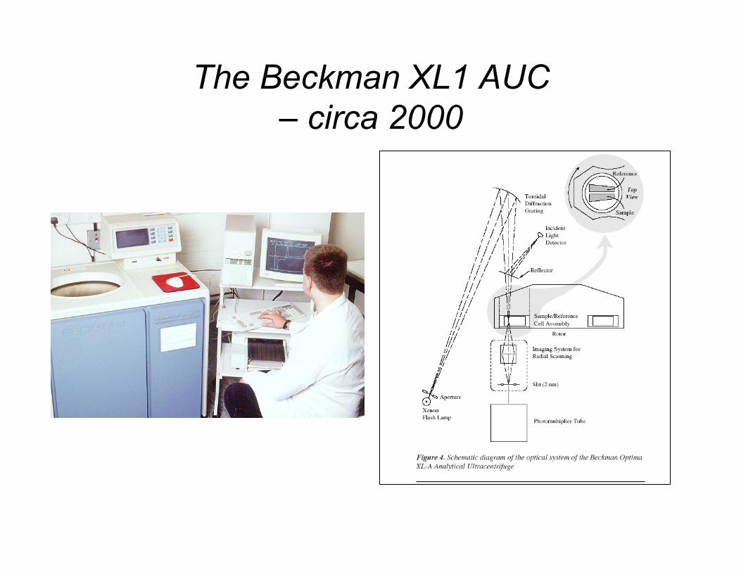
The Beckman XL1 AUC – circa 2000
Sedimentation Velocity - History Theodore Svedberg was awarded the 1926 Nobel Prize in Chemistry for
“for his work on disperse systems”
The (Theodor) Svedberg The Nobel Prize in Chemistry 1926. Nobelprize.org. 26 Feb 2012 http://www.nobelprize.org/nobel_prizes/chemistry/laureates/1926/
The Svedburg (by Isaac Grunewald) Uppsala University Art Collec>on. 2010 MinnesskriE. Royal Swedish Academy of Engineering Sciences (IVA)
UltraScan Website Borris Demeler
http://ultrascan.uthscsa.edu/index.php
Sedimentation Velocity Interference fringes vs. time & radial position
‘Fringe number’ (the number of fringes that cross a horizontal axis) is proportional to the solute (macromolecule or particle) concentration.
When the fringes are horizontal, the concentration is steady (~constant). When the fringes turn vertical, the macromolecule concentration is changing rapidly. These are boundaries between regions that contain particles and are depleted of particles.
In the series of interference patterns shown at right, the sample chamber has a uniform distribution (concentration) of particles at the beginning of the experiment (t = 0.0). As a function of time, three boundaries move away from the top of the sample column (at left, r ~ 6.7 cm) at different rates. The fastest moving boundary corresponds to a component in the sample with the largest sedimentation coefficient, s, the slowest moving boundary is characterized by the smallest value of s.
Note that rate of movement of the boundaries increases as the radial position of the boundary becomes larger.
Ff = -‐fv (fric>on force, viscous drag)
m
Fs = ω2rm (sedimenta>on force)
downward velocity, v Fb = -‐ω2rm0 = -‐ω2rmvρ (force of solvent displacement, buoyancy)
Fs + Fb + Ff = 0
!!!! "!""!!!!" "!" !!" =" "#
! !"!"!"( )!#" "!" #!" =" "$
! !"!"!"( )"
"=" " #!$#
"""$
! !"!"!"( )"#
"=" " #!$$
"""%
In the sedimenta>on velocity experiment, the forces ac>ng on a par>cle add to zero, due to the fact that viscous drag (Ff) grows in propor>on to the par>cle velocity.
Collec>ng the terms that relate to the par>cle on the leE hand side and those that relate to the experimental condi>ons on the other, leads to the defini>on of the sedimenta>on coefficient, s. s equals the velocity divided by the centrifugal accelera>on.
m = mass (grams) r = radial position (cm) ω = angular velocity (radians/s) v = partial specific volume of particle (cm3/g) ρ = solvent density (g/cm3) f = friction coefficient (g/s)
M = molecular weight (grams/mole) N = Avogadro’s number (particles/mole) v = sedimentation velocity (cm/s) s = sedimentation coefficient (s)
!" =" " !"#!#"=""#!$$
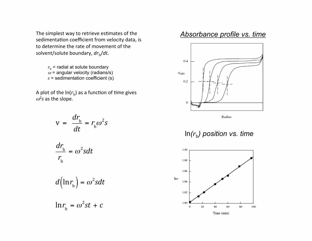
The simplest way to retrieve es>mates of the sedimenta>on coefficient from velocity data, is to determine the rate of movement of the solvent/solute boundary, drb/dt.
A plot of the ln(rb) as a func>on of >me gives ω2s as the slope.
rb = radial at solute boundary ω = angular velocity (radians/s) s = sedimentation coefficient (s)
Absorbance profile vs. time
ln(rb) position vs. time
!"!"!"="!##!$
! !""#( )$=$!%#!$
!"!# $=$!%"# $+$$
comparing values of s Since the sedimenta>on coefficient depends on solvent density and viscosity, standard condi>ons are necessary to compare the sedimenta>on coefficients determined for the same molecule by different inves>gators (under different condi>ons), or to make comparisons among different par>cles, where it is probable that s was determined under different condi>ons.
These standard condi.ons are 20oC in water as the solvent.
!!"#$ % =% %!&#'(!!"!"#$( )(!!"&#'( )
!&#'( )!&#$( )
!&#$( )!!"#$( )
!!"#$ % =% %!&#'(!!"!"#$( )(!!"&#'( )
!&#'( )!!"#$( )
!!"#$ % =% %!&#'(!!"( )!"#$(!!"( )&#'
!&#'( )!!"#$( )
S20,w = sedimentation coefficient in water at 20oC ST,b = sedimentation coefficient in buffer at ToC η20,w = viscosity of water at 20oC ηT,b = viscosity of buffer at ToC ρ20,w = density of water at 20oC ρT,b = density of buffer at ToC v = partial specific volume of particle (cm3/g)
The par>al specific volume of the par>cle does not change much with temperature or buffer; also these dependences usually aren’t known. The usual correc>ons are made to ρ and η, which are measured (or looked up in tables) as a func>on of temperature and solvent composi>on.
Sedimentation Equilibrium - History
Jean Baptiste Perrin "Jean Baptiste Perrin - Biography". Nobelprize.org. 26 Feb 2012 http://www.nobelprize.org/nobel_prizes/physics/laureates/1926/perrin.html
Jean Baptiste Perrin was awarded the 1926 Nobel Prize in Physics for “for his work on the discontinuous structure of matter, and especially for
his discovery of sedimentation equilibrium”
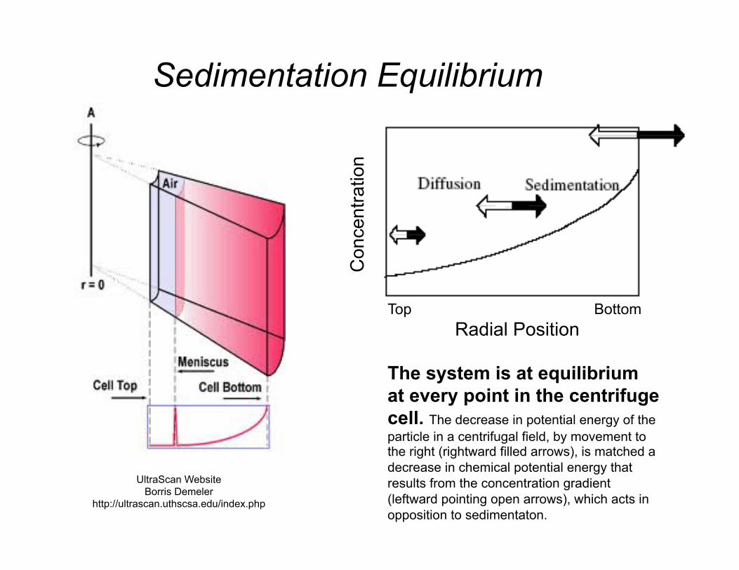
Sedimentation Equilibrium
Con
cent
ratio
n
Top Bottom Radial Position
UltraScan Website Borris Demeler
http://ultrascan.uthscsa.edu/index.php
The system is at equilibrium at every point in the centrifuge cell. The decrease in potential energy of the particle in a centrifugal field, by movement to the right (rightward filled arrows), is matched a decrease in chemical potential energy that results from the concentration gradient (leftward pointing open arrows), which acts in opposition to sedimentaton.
At equilibrium, the total chemical poten>al energy of a par>cle in a centrifugal field is the sum of the chemical poten>al energy and the poten>al energy contributed by the centrifugal field. As a condi>on of equilibrium, the total chemical poten>al energy is constant throughout the cell, a minimum, which means that the deriva>ve of the total poten>al, with respect to r, is zero.
!"!#! =! !"
!µ! ! =! !µ! !!!"#"!!
#!#
µi = total potential energy of the solute (or µ2) µi = chemical potential energy of the solute (or µ2) Mi = molecular weight of solute (M2) ω = angular velocity (radians/s) r = radial position (cm) Ci = solute concentration (molarity)
~ ~
! !µ!"#
! ! =! ! "µ!"#
!!!$!!"! !!=!!#
!µ"!#
! ! =! ! !µ"!$
"
#$$
%
&''% "&"
!$!#!!+!! !µ"
!%
"
#$$
%
&''$ "&"
!%!#!+!! !µ"
!&"
"
#$$
%
&''% "&"
!&"!#
1st term = 0 (isothermal conditions)
2nd term: !µ!!"
"
#$$
%
&''# !$!
%"%&""="" #!( )!"$& ""=""%!!' !"
$!&
µ! ! ! =! !µ!" !!+!!#$ "#%!
3rd term, assume ideal solution
!µ!!"!
"
#$$
%
&''# !$
" " =" " %$"!
Total Chemical Potential Energy in the Sedimentation Equilibrium Experiment
Total Chemical Potential Energy in the Sedimentation Equilibrium Experiment
! !µ"!#
! ! =! ! !µ"!#
!!!$"!"# !!=!!#
!"#$
%#$%&!+!"$$' $!"
#& !!!($"#& !!=!!$
!!! "#!#" !!( )!$# #!#$%&!
'&!'####=##%
!!"#"#!!!=!!
"## #!!!$ #!( )!$%
&'!%
! ! "#"#( )"# $%&
"# $$ &
! !!!=!!'## (!"!% #!( )!)$
&'$%
$
! !$
!" !"##$!"#%$!
"##
$
%&&&&&=&&
'"" (&'&$ "!( )!)
)!" #) &'&#%)( )
!"!#"##=##!"!$"%&'("" )#!#$ "!( )!*
*!" #* #!##$*( )"
#
$$
%
&
''
The equilibrium distribu>on of the par>cle concentra>on in the centrifuge cell varies exponen>ally on the radius. The molecular weight of the par>cle is determined in a shape-‐independent manner.