Equity in the Time Series, Part 2 - SJTU

15.433 Financial Markets Equity in the Time Series, Part 2

Equity in the Time Series, Part 2

15.433 Financial Markets

October 3 & 5, 2017

This Version: September 26, 2017

Fall 2017 Jun Pan, MIT Sloan –1–


Outline

• Volatility models and market risk measurement.

• Estimating volatility using financial time series:

– SMA: simple moving average model (traditional approach).

– EWMA: exponentially weighted moving average model (RiskMetrics).

– ARCH and GARCH models (Nobel Prize).

• EWMA for covariances and correlations.

• Portfolio volatility and Value-at-Risk.



What have we learned about the aggregate stock market?

• It is pervasive, the single most important risk factor in the equity world.

• It yields a positive risk premium, but the risk premium is difficult to

measure with precision because of

– the “high” level of stock market volatility

– and the limited length of the historical data.

• There is some evidence that the expected returns are time varying. The

autocorrelation of the aggregate stock returns is slightly positive, and the

dividend-to-price ratio has some predictability for future stock returns.

• Overall, only a small portion of future stock returns can be predicted (low

R-squared’s), and much of the uncertainty is unpredictable.



The volatility of the aggregate stock market

• Historical data can be used to measure volatility with much better

precision. Between risk and return, risk is something we can collect

more information about.

• In fact, we can learn about market volatility not only from the historical

stock market data (backward looking), but also from derivatives prices

(forward looking).

• Academics have made much progress in both directions, and

practitioners have adopted many of the ideas developed by academics.

• We will study three volatility estimators:

– SMA: simple moving average model (traditional approach).

– EWMA: exponentially weighted moving average model (RiskMetrics).

– ARCH and GARCH models (Nobel Prize).



The importance of measuring market volatility

• Portfolio managers performing optimal asset allocation.

• Risk managers assessing portfolio risk (e.g., Value-at-Risk).

• Derivatives investors trading non-linear contracts with values linked

directly to market volatility.

• Increasingly, the level of market volatility (e.g., VIX) has become a

market indicator (“the fear gauge”) watched closely by almost all

institutional investors, including those who are not trading directly in the

U.S. equity or U.S. equity derivatives markets.



1950

1951

195219531954

19551956

19571958 1 9 59

1960

19

6119621963

19641 9 65 196

619

6719

6819

6919

7019

7119

7219

73

1974 19751976

19771978

19791980

19811982

19831984

1985 1986 1987

1988

1989

1990

1991

1992

1993

1994

1995

1996

1997 1998 1999

20002001

20022003

20042005

20062007

20082009

Modern Finance

Portfolio Theory(Markowitz)

Two-Fund Separation(Tobin)

Investments and Capital Structure(Modigliani and Miller)

CAPM(Sharpe)

Behavior of Securities Prices (Samuelson)First Major Study of Mutual Funds (Jensen)

Efficient Markets Hypothesis (Fama)

Birth of Index Funds(McQuown)

Option Pricing Theory(Black, Scholes, Merton)

First US OptionsExchange, CBOE

Index MutualFunds (Bogle)

Rise ofJunk Bonds

Crash

S&L Bailout

Collapse ofJunk Bonds

LargeDerivativesLosses

LTCM

Enron

.comPeak

.comBottom

OTC Derivatives (e.g. interest-rate swaps)

Index Futures

Mortgage-BackedSecurities

Credit Derivatives (e.g. CDS)

�TIPS



1869

1880

1882

1906

1907

1913

1921

1927

1928

1929 1930 1930-40’s

1947-531956

19691970

19761981

1986

1987 1990 1993 1994

1994

1995

1998

1999

2000

2006

The Evolution of an Investment Bank

Marcus GoldmanBuy/Sell Commercial Papers

Firm Capital: $100K

Goldman+Sachs

Sears IPOLead Underwriterwith Lehman

Financial Panic

Federal Reserve Act

Proliferation ofInvestment Trusts;

Cheap & easy creditfuels leverage

Goldman SachsTrading Corporation Crash

Sidney Weinberg takes over (builds Investment Banking Business)Time of verylittle business andvirtually no profits

Gov’t antitrust caseagainst 17 banks

Lead Underwriterof Ford IPOGus Levy takes over(builds risk arbitrage business)Penn Central BankruptcyCommercial Paper ScandalWhitehead and Weinberg14 business principles“Our clients’ interestsalways come first”Acquired J. Aron(commodity)Hires from Salomon

(fixed income)

Freeman, head ofrisk arbitragearrested for insider trading

Rubin and Friedman

Record year in trading profitsHuge trading losses in FICC

Corzine and Paulson

Firm-widerisk management

LTCM crisisIPO withdrawn

IPO; CEO Paulson

Acquired SLK(NYSE specialist)

CEOBlankfein



Some losses on derivatives positions by non-financial corporations in mid-1990s

Orange County: $1.7 billion, leverage (reverse repos) and structured notes

Showa Shell Sekiyu: $1.6 billion, currency derivatives

Metallgesellschaft: $1.3 billion, oil futures

Barings: $1 billion, equity and interest rate futures

Codelco: $200 million, metal derivatives

Proctor & Gamble: $157 million, leveraged currency swaps

Air Products & Chemicals: $113 million, leveraged interest rate and currency swaps

Dell Computer: $35 million, leveraged interest rate swaps

Louisiana State Retirees: $25 million, IOs/POs

Arco Employees Savings: $22 million, money market derivatives

Gibson Greetings: $20 million, leveraged interest rate swaps

Mead: $12 million, leveraged interest rate swaps



Measuring Market Risk

• By the early 1990s, the increasing activity in securitization and the

increasing complexity in the financial instruments made the trading

books of many investment banks too complex and diverse for the chief

executives to understand the overall risk of their firms.

• Market risk management tools such as Value-at-Risk are ways to

aggregate the firm-wide risk to a set of numbers that can be easily

communicated to the chief executives. By the mid-1990s, most Wall

Street firms have developed risk measurement into a firm-wide system.

• Daily estimates of market volatility, along with correlations across

financial assets, constitute the key inputs to Value-at-Risk. JP Morgan’s

RiskMetrics uses exponentially weighted moving average (EWMA) model

to estimate the volatilities and correlations of over 480 financial time

series in order to construct a variance-covariance matrix of 480x480.















Estimating volatility using financial time series

• SMA: simple moving average model (traditional approach).

• EWMA: exponentially weighted moving average model (RiskMetrics).

• ARCH and GARCH models (Nobel Prize).



1970 1980 1990 2000 2010−25

−20

−15

−10

−5

0

5

10

15

1962−2015

mean

std

0.03%

1.01%

1962−2006

0.03%

0.93%

Daily Returns of the S&P 500 Index



The Simple Moving Average Model

• Unlike expected returns, volatility can be measured with better precision

using higher frequency data. So let’s use daily data.

• Some have gone into higher frequency by using intra-day data. But

micro-structure noises such as bid/ask bounce start to dominate in the

intra-day domain. So let’s not go there in this class.

• Suppose in month t, there are N trading days, with Rn denoting n-th

day return. The simple moving average (SMA) model:

σ =

√√√√ 1

N

N∑n=1

(Rn)2

• To get an annualized number: σ ×√252. (252 trading days per year).



Whether or not to take out μ?

• The industry convention is such that (Rt − μ)2 is replaced by R2t in the

volatility calculation.

• The reason is that, at daily frequency, μ2 is too small compared with

E(R2). Recall, μ is several basis points while σ is close to 1%.

• So instead of going through the trouble of doing E(R2)− μ2, people

just do E(R2).



Volatility estimates using the simple moving average (SMA) model

1970 1980 1990 2000 20100

10

20

30

40

50

60

70

80

90

100 Annualized Volatility (%)



How precise are SMA volatility estimates?

1970 1980 1990 2000 20100

20

40

60

80

100

120

140 A

nn

ual

ized

Vo

lati

lity

(%)

SMA estimates of σ and their 95% confidence intervals

95% Confidence, Upper

95% Confidence, Lower



What about SMA mean estimates?

1970 1980 1990 2000 2010−4

−3

−2

−1

0

1

2 M

on

thly

Ave

rag

e o

f D

aily

Ret

urn

s (%

)

SMA estimates of μ and their 95% confidence intervals

95% Confidence, Upper

95% Confidence, Lower



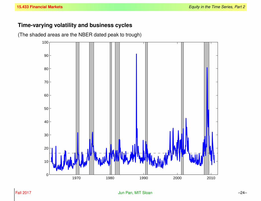
Why does volatility change over time?

• If the rate of information arrival is time-varying, so is the rate of price

adjustment, causing volatility to change over time.

• The time-varying volatility of the market return is related to the

time-varying volatility of a variety of economic variables, including

inflation, unemployment rate, money growth and industrial production.

• Stock market volatility increases with financial leverage: a decrease in

stock price causes an increase in financial leverage, causing volatility to

increase.

• Investors’ sudden changes of risk attitudes, changes in market liquidity,

and temporary imbalance of supply and demand could all cause market

volatility to change over time.



Time-varying volatility and business cycles

(The shaded areas are the NBER dated peak to trough)

1970 1980 1990 2000 20100

10

20

30

40

50

60

70

80

90

100



SMA vs. Option-Implied

1990 2000 20100

20

40

60

80

100

120

140

160 A

nn

ual

ized

Vo

lati

lity

(%)

SMA Vol Estimator CBOE VXO



VXO vs. VIX

1985 1990 1995 2000 2005 20100

20

40

60

80

100

120

140

160 A

nn

ual

ized

Vo

lati

lity

(%)

CBOE VXOCBOE VIX



Exponentially weighted moving average model

• The simple moving average (SMA) model fixes a time window and

applies equal weight to all observations within the window.

• In the exponentially weighted moving average (EWMA) model, the more

recent observation carries a higher weight in the volatility estimate.

• The relative weight is controlled by a decay factor λ.

• Suppose Rt is today’s realized return, Rt−1 is yesterday’s, and Rt−n is

the daily return realized n days ago. Volatility estimate σ:

Equally Weighted Exponentially Weighted√√√√ 1

N

N−1∑n=0

(Rt−n)2

√√√√(1− λ)N−1∑n=0

λn (Rt−n)2



100 90 80 70 60 50 40 30 20 10 0

0.1

0.2

0.3

0.4

0.5

0.6

0.7

0.8

0.9

1

days in the past

weight on past observations

λ=0.8

λ=0.94

λ=0.97



Source: RiskMetrics—Technical DocumentFall 2017 Jun Pan, MIT Sloan –29–


SMA and EWMA Estimates after a Crash

Source: J.P.Morgan/Reuters RiskMetrics — Technical Document, 1996



Computing EWMA recursively

• One attractive feature of the exponentially weighted estimator is that it

can be computed recursively.

• You will appreciate this convenience if you have to compute the EWMA

volatility estimator in Excel.

• Let σt be the EWMA volatility estimator using all the information available

on day t− 1 for the purpose of forecasting the volatility on day t.

• Moving one day forward, it’s now day t. After the day is over, we observe

the realized return Rt.

• We now need to update our EWMA volatility estimator σt+1 using the

newly arrived information (i.e. Rt). It turns out that we can do so by

σ2t+1 = λσ2

t + (1− λ)R2t



What about the first observation?

• The recursive formula has to start from the beginning:

σ22 = λσ2

1 + (1− λ)R21

So what to use for σ1?

• In practice, the choice of σ1 does not matter in any significant way after

running the iterative process long enough:

σ23 = λσ2

2 + (1− λ)R22

= λ2 σ21 + (1− λ)

(λR2

1 +R22

)σ24 = λσ2

3 + (1− λ)R23

= λ3 σ21 + (1− λ)

(λ2R2

1 + λR22 +R2

3

). . .

σ2t = λt−1 σ2

1 + (1− λ)(λt−2R2

1 + . . .+ R2t−1

)Fall 2017 Jun Pan, MIT Sloan –32–


• A good idea is to have the iterative process run for a while (say a few

months) before recording volatility estimates.

• (Prof. Pan’s Choice:) I like to set σ1 =std(R), which is the

“unconditional” or sample standard deviation of R. The logic is that if I

don’t have any information about σ1 at the beginning of the volatility

estimation, I might as well use the unconditional estimate of σ.

• (The industry practice:) It is typical to set σ22 = R2

1 and start the

recursive process from σ3. The rationale is that σ1 is unknowable and

the only data we have at time 1 is R1. So R21 is our best estimate for σ2

2 .

This approach is adopted by most of the practitioners, including

RiskMetrics.



Dating Convention for σt

• The dating convention adopted by most people:

σ2t+1 = λσ2

t + (1− λ)R2t

The rationale is that this σ is estimated for the purpose of forecasting the

next period’s volatility. So it should be dated as σt+1.

• (Prof. Pan’s Choice:) I actually like to use

σ2t = λσ2

t−1 + (1− λ)R2t

The rationale is that at time t, I am forming an estimate σt using all of

the information available to me at time t.

• I will always use the main-stream approach and date it by σt+1.



Decay factor, Strong or Weak?

• A strong decay factor (that is, small λ) underweights the far away events

more strongly, making the effective sample size smaller.

• A strong decay factor improves on the timeliness of the volatility

estimate, but that estimate could be noisy and suffers in precision.

• On the other hand, a weak decay factor improves on the smoothness

and precision, but that estimate could be sluggish and slow in response

to changing market conditions.

• So there is a tradeoff.



2007 2008 2009 2010 20110

20

40

60

80

100

120

year

An

nu

aliz

ed V

ola

tilit

y (%

)

Annualized EWMA Volatility Estimate using Daily S&P 500 Index Returns

λ=0.8λ=0.94



2007 2008 2009 2010 20110

10

20

30

40

50

60

70

80

year

An

nu

aliz

ed V

ola

tilit

y (%

)

Annualized EWMA Volatility Estimate using Daily S&P 500 Index Returns

λ=0.97λ=0.94



Picking the optimal decay factor based on volatility forecast

• RiskMetrics sets λ = 0.94 in estimating volatility and correlation. One of

their key criteria is to minimize the forecast error.

• We form σt+1 on day t in order to forecast the next-day volatility. So after

observing Rt+1, we can check how good σt+1 is in doing its job.

• This leads to the daily root mean squared prediction error

RMSE =

√√√√ 1

T

T∑t=1

(R2

t+1 − σ2t+1

)2• The deciding factor of RMSE is our choice of λ. For my running example

(daily S&P 500 index returns 2007-2010):

λ 0.80 0.9075∗ 0.94 0.97

RMSE 8.1844 8.0124 8.0544 8.2444



Maximum Likelihood Estimation

• The gold standard in any estimation is maximum likelihood estimation,

because it is the most efficient method. So let’s see what MLE has to say

about the optimal λ.

• We assume that conditioning on the volatility estimate σt+1, the stock

return Rt+1 is normally distributed:

f (Rt+1|σt+1) =1√

2πσt+1

e−

R2t+1

2σ2t+1

• Take natural log of f :

ln f (Rt+1|σt+1) = − ln σt+1 −R2

t+1

2σ2t+1

I dropped 2π since it will not affect anything we will do later.



• We now add them up to get what econometricians call log-likelihood (llk):

llk = −T∑t=1

(ln σt+1 +

R2t+1

2σ2t+1

)

• The only deciding factor in llk is our choice of λ. It turns out that the best

λ is the one that maximizes llk.

• In practice, we take -llk and minimize -llk instead of maximizing llk.

• For my running example (daily S&P 500 index return 2007-2010), I find

the optimal λ that minimizes -llk is 0.9320. Not exactly the same as the

optimal λ of 0.9075 that minimizes RMSE, but these two are reasonably

close.



The Surface of Planet MLE

0.8 0.82 0.84 0.86 0.88 0.9 0.92 0.94 0.96 0.98 1800

820

840

860

880

900

920

940 −

llk

λ



The ARCH and GARCH models

• The ARCH model, autoregressive conditional heteroskedasticity, was

proposed by Professor Robert Engle in 1982. The GARCH model is a

generalized version of ARCH.

• ARCH and GARCH are statistical models that capture the time-varying

volatility:

σ2t+1 = a0 + a1R

2t + a2 σ

2t

• As you can see, it is very similar to the EWMA model. In fact, if we set

a0 = 0, a2 = λ, and a1 = 1− λ, we are doing the EWMA model.

• So what’s the value added? This model has three parameters while the

EWMA has only one. So it offers more flexibility (e.g., allows for mean

reversion and better captures volatility clustering).

• But I think EWMA is good enough for us, for now.





EWMA covariances and correlations

• Our goal is to create the variance-covariance matrix for the key risk

factors influencing our portfolio.

• For the moment, let’s suppose that there are only two risk factors

affecting our portfolio.

• Let RAt and RB

t be the day-t realized returns of these two risk factors.

The covariance between A and B:

covt+1 = λ covt + (1− λ)RAt ×RB

t

• And their correlation:

corrt+1 =covt+1

σAt+1σ

Bt+1

,

where σAt+1 and σB

t+1 are the EWMA volatility estimates.



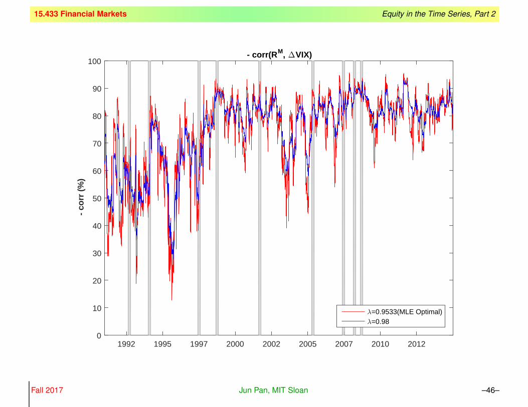
The negative correlation between RM and ΔV IX

• Monthly returns RMt on the stock market portfolio is highly negatively

correlated with monthly changes in VIX: -69.41%.

• Now let’s apply our EWMA approach, which will give us a time-series of

correlations between these two risk factors.

• We see an interesting time-series pattern of the negative correlation

between daily stock returns and daily changes in VIX.

• In particular, this correlation has become more negative in recent years.

• (CBOE started to offer futures trading on VIX on March 26, 2004.)



1992 1995 1997 2000 2002 2005 2007 2010 20120

10

20

30

40

50

60

70

80

90

100

- c

orr

(%

)

- corr(RM, ΔVIX)

λ=0.9533(MLE Optimal)λ=0.98



0

20

40

60

80

100

120

140

160C

BO

E V

IX (

%)

The CBOE Volatility Index (pre-1990: VXO; post-1990: VIX)

1986 1988 1990 1992 1994 1996 1998 2000 2002 2004 2006 2008 2010 2012 2014 2016200

400

600

800

1000

1200

1400

1600

1800

2000

2200

S&

P 5

00 In

dex

Leve

l



Calculating Volatility for a Portfolio

• Suppose that our portfolio has two important risk factors, whose daily

returns are RA and RB , respectively.

• Performing risk mapping using individual positions, the portfolio weights

on these two risk factors are wA and wB .

• Let’s focus only on the risky part of our portfolio and leave out the cash

part. So let’s normalize the weights so that wA + wB = 1. Let’s

assume our risk portfolio has a market value of $100 million today.

• We apply EWMA to get time-series of their volatility estimates σAt and

σBt , and correlation estimates ρAB

t . And our portfolio volatility is

σ2t = w2

A× (σAt )

2+w2B × (σB

t )2+2×wA×wB × ρAB

t ×σAt ×σB

t

• It is in fact easier to do this calculation using matrix operations,

especially when you have to deal with hundreds of risk factors.



Variance-Covariance Matrix

• We construct a variance-covariance matrix for risk factors A and B:

Σt =

((σA

t )2 ρAB

t σAt σ

Bt

ρABt σA

t σBt

(σBt

)2)

• It is a 2×2 matrix, since we have only two risk factors. If you have 100

risk factors in your portfolio, then you will have a 100×100 matrix. For

example, in JPMorgan’s RiskMetrics, 480 risk factors were used. In

Goldman’s annual report, 70,000 risk factors were mentioned.

• A risk manager deals with this type of matrices everyday and the

dimension of the matrix can easily be more than 100, given the

institution’s portfolio holdings and risk exposures.

• Notice the timing: for σt, we use all returns up to day t− 1 for the

purpose of forecasting volatility for day t.



Portfolio Volatility

• Let’s write our weights in vector form, time stamped by today, t-1,

wt−1 =

(wA

t−1

wBt−1

)

• Our portfolio volatility is

σ2t =

(wA

t−1 wBt−1

)×(

(σAt )

2 ρABt σA

t σBt

ρABt σA

t σBt

(σBt

)2)

×(wA

t−1

wBt−1

)

• Using the notation we’ve developed so far, we can also write

σ2t = w′

t−1 × Σt × wt−1 ,

which involves using mmult and transpose in Excel.



Portfolio VaR

• Let σ be the daily volatility estimate of the portfolio. Then the 95%

one-day VaR is,

VaR = portfolio value × 1.645× sigma

• The 99% tail event corresponds to a -2.326σ move away from the mean.

The 95% tail event corresponds to -1.645σ.

99% 95%

-4 -3 -2 -1 0 1 2 3 4



• Assuming the market value of our risk portfolio is $100 million, the

one-day loss in portfolio value associated with the 5% worst-case

scenario is

$100M × 1.645× σ

• Suppose that we have only one risk factor, which is the S&P 500 index. If

today is a normal day with an average volatility around 1%, then the

one-day 95% VaR is $1.645M. For the same portfolio value, if the

reported VaR is much higher than $1.645M, then today must be a

volatile day.

• Overall, if we fix our VaR estimate to a certain horizon, say daily, then the

main drivers to the VaR estimates are: the market value and volatility of

our portfolio. A reduction in VaR could be caused by a reduction in the

market value (either by active risk reduction or passive loss in market

value) or a reduction in market volatility.



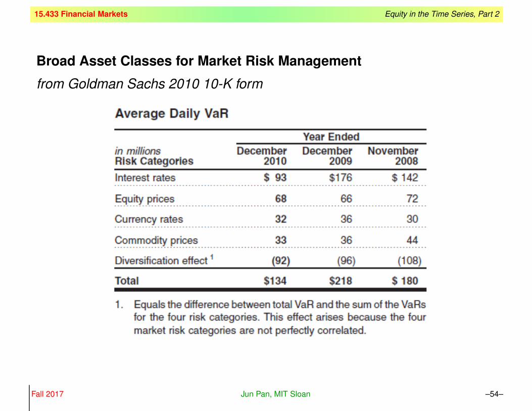
Key Asset Classes for Market Risk Management

• What JP Morgan RiskMetrics had to offer (free of charge) back in 1996

gives a good overall picture of what kind of asset classes are involved in

calculating the market risk exposure of an investment bank.

• RiskMetrics data sets: Two sets of daily estimates of future volatilities

and correlations of approximately 480 rates and prices, with each data

set totaling 115,000+ data points. One set is for computing short-term

trading risks, the other for medium term investment risks. The data sets

cover foreign exchange, government bond, swap, and equity markets in

up to 31 currencies. Eleven commodities are also included.

• This set of data (equity, currency, interest rates, and commodity) is very

much the domain of Market Risk Management. In addition, Credit and

Liquidity Risk Management have become increasingly important. For

this, good data, models, and talents on credit and liquidity are in need.



Broad Asset Classes for Market Risk Management

from Goldman Sachs 2010 10-K form


Date post:	17-Mar-2022
Category:	Documents
Upload:	others
View:	1 times
Download:	0 times

Equity in the Time Series, Part 2 - SJTU

Documents