JSS Journal of Statistical Software February 2008, Volume 24, Issue 3. http://www.jstatsoft.org/ ergm: A Package to Fit, Simulate and Diagnose Exponential-Family Models for Networks David R. Hunter Penn State University Mark S. Handcock University of Washington Carter T. Butts University of California, Irvine Steven M. Goodreau University of Washington Martina Morris University of Washington Abstract We describe some of the capabilities of the ergm package and the statistical theory underlying it. This package contains tools for accomplishing three important, and inter- related, tasks involving exponential-family random graph models (ERGMs): estimation, simulation, and goodness of fit. More precisely, ergm has the capability of approximating a maximum likelihood estimator for an ERGM given a network data set; simulating new network data sets from a fitted ERGM using Markov chain Monte Carlo; and assessing how well a fitted ERGM does at capturing characteristics of a particular network data set. Keywords : exponential-family random graph model, Markov chain Monte Carlo, maximum likelihood estimation, p-star model. 1. Introduction The ergm package for R (R Development Core Team 2007), a cornerstone of the statnet suite of packages for statistical network analysis, provides tools for modeling networks based on a well-studied class of models called exponential-family random graph models (ERGMs) or p-star models (Holland and Leinhardt 1981; Wasserman and Pattison 1996; Robins, Pattison, Kalish, and Lusher 2007a). In particular, the package allows users to obtain approximate (or, in some cases, exact) maximum likelihood estimates (MLEs); simulate random networks from a specified ERGM; and perform graphical goodness-of-fit checks of the type described by Hunter, Goodreau, and Handcock (2008). This article describes some of the technical
We describe some of the capabilities of the ergm package and the statistical theoryunderlying it. This package contains tools for accomplishing three important, and inter-related, tasks involving exponential-family random graph models (ERGMs): estimation,simulation, and goodness of fit. More precisely, ergm has the capability of approximatinga maximum likelihood estimator for an ERGM given a network data set; simulating newnetwork data sets from a fitted ERGM using Markov chain Monte Carlo; and assessinghow well a fitted ERGM does at capturing characteristics of a particular network dataset.
Keywords: exponential-family random graph model, Markov chain Monte Carlo, maximumlikelihood estimation, p-star model.
1. Introduction
The ergm package for R (R Development Core Team 2007), a cornerstone of the statnet suiteof packages for statistical network analysis, provides tools for modeling networks based ona well-studied class of models called exponential-family random graph models (ERGMs) orp-star models (Holland and Leinhardt 1981; Wasserman and Pattison 1996; Robins, Pattison,Kalish, and Lusher 2007a). In particular, the package allows users to obtain approximate(or, in some cases, exact) maximum likelihood estimates (MLEs); simulate random networksfrom a specified ERGM; and perform graphical goodness-of-fit checks of the type describedby Hunter, Goodreau, and Handcock (2008). This article describes some of the technical
2 ergm: Fit, Simulate and Diagnose Exponential-Family Models for Networks
background and algorithms that drive the ergm package.
1.1. Obtaining ergm
Because the ergm package is part of the statnet suite of packages, it may be obtained andloaded by loading the statnet suite as described in Goodreau, Handcock, Hunter, Butts,and Morris (2008a) or at the statnet project Web site at http://statnetproject.org/.Alternatively, a user may choose to install and load just the ergm package itself in R via
R> install.packages("ergm")
R> library("ergm")
(Throughout this article, R input is represented by italicized typewriter font beginning withthe R> prompt, or the + prompt if it is a continuation of a previous line.) Because the ergmpackage depends on the network package (Butts 2008), the lines above will automaticallyinstall (if necessary) and load the network package as well. All of these packages are availablefrom the Comprehensive R Archive Network (CRAN) at http://CRAN.R-project.org/, andfurther information about them may be obtained from the statnet Web site at http://statnetproject.org/.
1.2. License and citation information
The ergm package is free and open-source, and released under GPL-3 with attribution re-quirements for the software and its source code. To obtain license information go to http://statnetproject.org/attribution/.
Please cite the ergm package when you use it for research that is published or otherwise pub-licly distributed. Citation information is provided on our Web site at http://statnetproject.org/citation.shtml, and can be obtained by typing citation("ergm").
1.3. ERGMs in a nutshell
The purpose of ERGMs, in a nutshell, is to describe parsimoniously the local selection forcesthat shape the global structure of a network. To this end, a network dataset, like thosedepicted in Figure 1, may be considered like the response in a regression model, where thepredictors are things like “propensity for individuals of the same sex to form partnerships” or“propensity for individuals to form triangles of partnerships”. In Figure 1(b), for example, itis evident that the individual nodes appear to cluster in groups of the same numerical labels(which turn out to be students’ grades, 7 through 12); thus, an ERGM can help us quantifythe strength of this intra-group effect. The information gleaned from use of an ERGM maythen be used to understand a particular phenomenon or to simulate new random realizationsof networks that retain the essential properties of the original. Handcock, Hunter, Butts,Goodreau, and Morris (2008) say more about the purpose of modeling with ERGMs; yet inthis article, we focus primarily on technical details.
In the remainder of the article, we introduce the two network datasets of Figure 1 that willbe used for illustrative purposes (Section 2), provide a brief technical summary of what anERGM is (Section 3), and list a few examples of ERGMs along with numerous references inwhich these models are developed more fully (Section 4). Section 5 describes the algorithm
Figure 1: The (a) samplike and (b) faux.mesa.high networks described in Section 2. Thevalues of nodal covariates may be indicated using various colors, shapes, and labels of nodes.
for producing approximate maximum likelihood estimates used by the ergm package, whileSections 6 and 7 describe the simulation and goodness-of-fit capabilities, respectively, of thepackage. The focus of this article is restricted to the technical aspects of modeling usingERGMs, so it does not provide a proper discussion of the purpose of ERGMs nor how bestto construct ERGMs in practice. There is a large body of literature on these topics, andthe interested reader might turn to the special issue of Social Networks (Robins and Morris2007), which contains several related articles and which provides extensive lists of references.Additional aid on the practical use of the statnet suite of packages is given by Goodreau et al.(2008a) in the form of a short tutorial.
2. Network datasets in ergm
Several network datasets are included with the ergm package. To see a list of them, type:
R> data(package = "ergm")
In this article, we use the samplike and faux.mesa.high networks, depicted in Figure 1,to illustrate various aspects of the ergm package functionality. To learn more about theseparticular datasets, or any of the datasets included with the ergm package, it is possible toview their corresponding documentation files by using the help function, or, equivalently, thequestion mark, as follows:
R> help("samplike")
R> ? "faux.mesa.high"
In the samplike dataset of Figure 1(a), each node represents a monk within a particularmonastery and a directed edge from one to another indicates that the first named the secondas one of the three monks he likes the most, at any of the three distinct time points when thesurvey was administered; type help("sampson") for more details. Three groups, identified
4 ergm: Fit, Simulate and Diagnose Exponential-Family Models for Networks
by Sampson (1968) after analyzing the trends in the pattern of ties over time, are indicated bythe three different shapes and colors of nodes. Note that the definition of group membershipin this case is endogenous: membership is not a measured attribute of the node, like age,that is independent of the relational structure, but instead a latent cluster defined by thestructure of relations. The default behavior of the plotting function for a directed networklike samplike is to place arrows at one end of each line segment, indicating the direction ofeach edge.
In the faux.mesa.high dataset of Figure 1(b), each node represents a student in grades seventhrough twelve at a hypothetical yet realistic school (or middle school-high school pair) inthe United States, and each edge indicates a mutual friendship in which each node namedthe other as one of his or her top five male or top five female friends; see the appendix inGoodreau et al. (2008a) for the origin of this data set. Boys are depicted by square nodes andgirls by many-sided polygons that appear circular; the label for each node indicates the gradein school (seventh through twelfth). In contrast to the samplike network, the nodal attributesin this case, grade and sex, are exogeneous. This difference means they can serve as predictorsin a generative model for the friendships. Since the edges indicate mutual friendships, this isan undirected network.
In both figures 1(a) and 1(b), it is evident that the colors used for displaying the nodesare related to the clustering of the nodes. However, the plotting function does not considerthese colors in any way when positioning the nodes; it only considers the pattern of edgesand non-edges that exist in the network. Since the colors in the samplike are derived fromthe pattern of edges, the clustering by color is tautological. The fact that the nodes fromfaux.mesa.high cluster by grades, however, is different. In this case the clustering revealsa qualitative fact about this network, and the ergm package allows us to analyze propertieslike this quantitatively. The exact R code used to produce both of these plots is given inAppendix A—note that, because the algorithm used for the plots has a random element, thiscode will not produce exactly the same layouts as in Figure 1.
3. ERGM specification
Let the random matrix Y represent the adjacency matrix of an unvalued (binary) networkand let Y denote the support of Y. Then we may think of Y as the set of all obtainablenetworks. Typically, as in this article, one fixes the number n of individuals, so that Y isa subset of all n × n matrices whose entries are all zero or one and whose diagonal entriesare all zero—since the (i, j) entry indicates an edge from i to j, forcing the diagonal to bezero means that self-partnerships are disallowed. In the undirected case, Y contains onlysymmetric matrices.
3.1. The model
The distribution of Y can be parameterized in the form
Pθ,Y(Y = y) =expθ>g(y)
κ(θ,Y), y ∈ Y, (1)
where θ ∈ Ω ⊂ Rq is the vector of model coefficients and g(y) is a q-vector of statisticsbased on the adjacency matrix y (Frank and Strauss 1986; Wasserman and Pattison 1996).
Journal of Statistical Software 5
Model (1) may be expanded by replacing g(y) with g(y,X) to allow for additional covariateinformation X about the network, as described in Section 4.3. The denominator,
κ(θ,Y) =∑z∈Y
expθTg(z), (2)
is the normalizing factor that ensures that Equation 1 is a legitimate probability distribution.Specification of Y, including the number of nodes, n, is an important yet often overlookedaspect of model (1). If, for instance, an edge denotes a heterosexual sexual relationship, theneach element of Y should contain certain structural zeros, namely, all Yij for which both i and jrepresent nodes of the same sex. At its largest, for a fixed n, Y may contain up to N = 2n(n−1)
networks, a very large number even for moderate-sized n, which makes calculation of κ(θ,Y)the primary barrier to inference using this model.
3.2. Change statistics
An alternative specification of the model (1) clarifies the interpretation of the θ coefficients.To articulate this alternative, we first introduce the notion of a vector of change statistics.Such a vector is a function of three things: A particular choice g(·) of statistics defined on anetwork, a particular network y, and a particular pair of different nodes (i, j) that is eitherordered or unordered, respectively, according to whether y is directed or undirected. Wedefine the vector of change statistics as
δg(y)ij = g(y+ij)− g(y−ij),
where y+ij and y−ij represent the networks realized by fixing yij = 1 or yij = 0, respectively,
while keeping all the rest of the network exactly as in y itself. In other words, δg(y)ij is thechange in the value of the network statistic g(y) that would occur if yij were changed from 0to 1 while leaving all of the rest of y fixed.
In terms of the change statistic vector, model (1) may be shown to imply the followingdistribution of the Bernoulli variable Yij , conditional on the rest of the network:
logit[Pθ,Y(Yij = 1|Yc
ij = ycij)]
= θ>δg(y)ij , (3)
where the logit function is defined by logit(p) = log[p/(1− p)] and Ycij represents the rest of
the network other than the single variable Yij . When the network statistics involve covariatesX in addition to y, as we will describe in Section 4.3, we may add X to the notation andwrite δg(y,X)ij .
Equation 3 reveals two facts: First, the probability on the left hand side depends on ycij onlythrough the change statistics δg(y)ij , not on g(y+
ij) or g(y−ij) themselves. In many cases, it ismuch easier to calculate δg(y)ij than it is to calculate g(y+
ij) or g(y−ij), and this fact can leadto efficient computational algorithms. As an example of this phenomenon, the Erdos-Renyimodel of Section 4.1 implies that δg(y)ij = 1 for all y and for all i and j.
Second, Equation 3 says that each component of the θ vector may be interpreted as theincrease in the conditional log-odds of the network, per unit increase in the correspondingcomponent of g(y), resulting from switching a particular Yij from 0 to 1 while leaving therest of the network fixed at Yc
ij . For examples of these kinds of interpretations for an actualdataset, refer to Sections 4 and 6 of Goodreau et al. (2008a).
6 ergm: Fit, Simulate and Diagnose Exponential-Family Models for Networks
The specific statistics that may be included in the g(y) vector in the ergm package are listedand described in Morris, Handcock, and Hunter (2008). In the next section, we illustratethe use of only a small fraction of the available terms on the samplike and faux.mesa.highdatasets. It is important to remember that because samplike is directed and faux.mesa.highis undirected, there are certain types of model terms that may not be used with one or the otherof these datasets. A summary of these restrictions may be found in the table in Appendix Aof Morris et al. (2008).
4. Examples of ERGMs
Here, we offer a brief glimpse at some important categories of ERGMs. We also give numerousreferences for readers interested in delving more deeply into the intricacies of building ERGMs,which is a subject that we cannot adequately cover given the limited space available and thelimited scope of this article.
4.1. Bernoulli and Erdos-Renyi models
In the remainder of this article, we take
Ω = θ ∈ Rq : κ(θ,Y) <∞
to be the parameter space. The dimension q of Ω is at most N − 1 (for the “saturated”model), although it is typically much smaller than this. For example, if the dyads Yij = Yjiof an undirected network are mutually independent and Y consists of the set of all possibleundirected networks, the model can be written
log [Pθ,Y(Y = y)] =∑∑i<j
θijyij − log κ(θ,Y), y ∈ Y, (4)
where θij = logit [Pθ,Y(Yij = 1)] is the log-odds of a tie in the (i, j) dyad and
log κ(θ,Y) =∑∑i<j
log[1 + expθij].
[Recall that the logit, or log-odds, function is defined by logit p = log p − log(1 − p).] Thus,for model (4), q = n(n− 1)/2 and the elements of the vector g(y) are just yij . This model isoften called a Bernoulli network. The special case where the dyads have a common probabilityimplies that q = 1, g(y) =
∑∑i<j yij is the number of partnerships in the network, and the
single coefficient θ can be interpreted as the common log-odds of partnership formation withinany dyad. The mathematical properties of this homogeneous Bernoulli network model, alsoknown as the Erdos-Renyi model, have been extensively studied—see Albert and Barabasi(2002) and the many references therein—but the simplicity and homogeneity that make ittractable also make it less useful as a realistic model for social phenomena.
Consider the samplike dataset, which is contained in the ergm package and which may beaccessed, once ergm is loaded, by typing
R> data("sampson")
Journal of Statistical Software 7
Some information about the dataset may be obtained by typing help("sampson") orhelp("samplike"). To obtain summary statistical information, we may type either samplikeor summary(samplike):
A directed network with eighteen vertices (nodes) could have up to 18 × 17 = 306 edges.Since this network has 88, we should expect the maximum likelihood estimator for θ in anErdos-Renyi model to equal logit (88/306) = −.90716. To verify this fact using the ergmpackage, we may use the following commands:
R> model1 <- ergm(samplike ~ edges)
R> model1$coef
edges-0.9071582
Note that the ergm command requires the formula format in R, much like other regression-like functions such as lm for linear regression or glm for generalized linear models. For ergm,the formula should be of the form
network object ~ <model term 1> + <model term 2> + ...
where the model terms determine the elements of the g(y) vector. The ergm function allowsmany possible model terms other than edges; a complete catalog is given in Morris et al.(2008).
4.2. The p1 model
Holland and Leinhardt (1981) appear to be the first to propose log-linear models for socialnetworks. Suppose that we take Y to be the set of all directed graphs, with independentdyads [i.e., the pairs (Yij , Yji) are independent for different choices of i, j] and the followingmodel for tie probabilities:
Pθ,Y(Yij = x, Yji = y) =
mij if x = y = 1aij if x = 1, y = 0nij if x = y = 0.
8 ergm: Fit, Simulate and Diagnose Exponential-Family Models for Networks
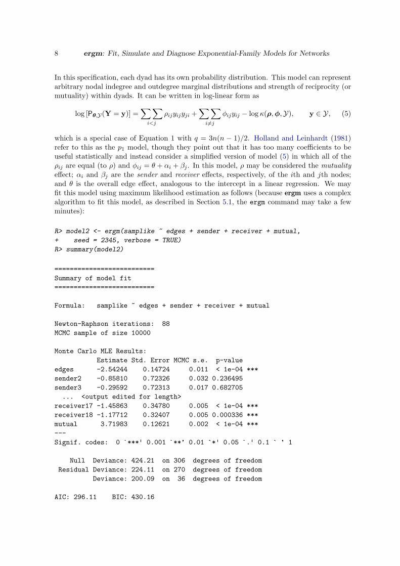
In this specification, each dyad has its own probability distribution. This model can representarbitrary nodal indegree and outdegree marginal distributions and strength of reciprocity (ormutuality) within dyads. It can be written in log-linear form as
log [Pθ,Y(Y = y)] =∑∑i<j
ρijyijyji +∑∑i 6=j
φijyij − log κ(ρ,φ,Y), y ∈ Y, (5)
which is a special case of Equation 1 with q = 3n(n − 1)/2. Holland and Leinhardt (1981)refer to this as the p1 model, though they point out that it has too many coefficients to beuseful statistically and instead consider a simplified version of model (5) in which all of theρij are equal (to ρ) and φij = θ + αi + βj . In this model, ρ may be considered the mutualityeffect; αi and βj are the sender and receiver effects, respectively, of the ith and jth nodes;and θ is the overall edge effect, analogous to the intercept in a linear regression. We mayfit this model using maximum likelihood estimation as follows (because ergm uses a complexalgorithm to fit this model, as described in Section 5.1, the ergm command may take a fewminutes):
Null Deviance: 424.21 on 306 degrees of freedomResidual Deviance: 224.11 on 270 degrees of freedom
Deviance: 200.09 on 36 degrees of freedom
AIC: 296.11 BIC: 430.16
Journal of Statistical Software 9
The seed argument is used here and elsewhere in the article to make the output exactlyreproducible, since the fitting algorithm is random; however, we have noticed that there existsome differences among the output produced by some platforms for some of the examplesnonetheless. We obtained these results using R version 2.6.2 on a Windows machine usingergm version 2.1 and network version 1.3. The verbose = TRUE argument results in a lotof output as the algorithm proceeds. The control = control.ergm(check.degeneracy =TRUE) option would have invoked a check for degeneracy that takes quite a bit of time forthis particular model due to the fact that it contains 36 parameters. Model degeneracy isdiscussed briefly by Handcock et al. (2008) in this volume, and in more detail by Handcock(2003b,a).
Note that summary(model1) produced a lot of information besides the coefficient estimates.The standard errors and loglikelihood values on which the deviance, AIC and BIC valuesare based use stochastic approximations discussed in Hunter and Handcock (2006). Also notethat there are only 17 sender effects (sender2 through sender18) and 17 receiver effects, eventhough there are 18 nodes. This is because inclusion of all 18 effects would result in a lineardependency among the statistics of g(y), which should be avoided here, as in all statisticalmodels.
The estimates above are approximate maximum likelihood estimates obtained using a stochas-tic algorithm based on Markov Chain Monte Carlo (MCMC); hence, the results will not beexactly the same for all runs. However, if exact reproducibility of coefficient estimates isimportant, it is possible to seed the random number generator manually using the seed argu-ment to the ergm function; type ?ergm for more details. In this particular case, the formula inEquation 1 simplifies considerably and it is possible using numerical methods to find the exactmaximum likelihood estimator, i.e., without resorting to a stochastic MCMC-based algorithm.Holland and Leinhardt (1981) do this, but unfortunately it is not possible to compare theirresults directly with ours because they use a slightly different dataset.
These early simple ERGMs, which have no exogeneous covariates and assume independenceacross dyads, have been substantially extended and generalized in subsequent social networkliterature. Based on developments in spatial statistics (Besag 1974), Frank and Strauss (1986)introduce forms of dependence with Markov structure. Wasserman and Pattison (1996) incor-porate exogeneous and endogenous nodal attributes (Pattison and Wasserman 1999) and makea distinction between explanatory and response variables (Robins, Pattison, and Wasserman1999), resulting in social influence (Robins, Pattison, and Elliott 2001b) and social selection(Robins, Elliott, and Pattison 2001a) models. These generalizations essentially allow anal-ysis of networks with “colors” on the nodes, where “color” is used to indicate the attributevalues conceptually as Figure 1 does literally. Recent developments include new forms of de-pendency structures, to take into account more general neighborhood effects. These modelsrelax the one-step Markovian dependence assumptions, allowing investigation of longer rangeconfigurations, such as longer paths in the network or larger cycles (Pattison and Robins2002). Models for bipartite (Faust and Skvoretz 1999) and tripartite (Mische and Robins2000) network structures have also been developed.
4.3. Exogenous covariates and dyadic independence
Attribute information is easily incorporated into an ERGM (Fienberg and Wasserman 1981).Suppose we wish to examine the impact of p exogenous attributes represented by an n ×
10 ergm: Fit, Simulate and Diagnose Exponential-Family Models for Networks
n × p array, X, whose ijkth element is the value of the kth attribute for the potential edgerepresented by the Bernoulli random variable Yij . Note that this construction allows theattributes to be functions of nodal covariates. For instance, Xijk might be the absolutedifference in ages between nodes i and j, say, |agei−agej |. As a practical matter, note in thisexample that it is not actually necessary to store the entire X array; it is much simpler tostore only the vector giving the age of each node along with a rule for how to calculate Xijk
when needed.
To modify the ERGM of Equation 1 to allow X to influence the probability distribution of Y,we replace g(y) by g(y,X), indicating that the statistics depend on the attribute informationin addition to the relationship information. As an example, suppose that g(y,X) includes thefollowing terms (where the equivalent ergm-package codings are given in square brackets):
# of edges in y [ergm code: edges]
# of edges between students of the same grade, counted separately for each possiblegrade [nodematch("Grade", diff = TRUE)]
# of edges involving males, with male-male edges counted twice [nodefactor("Sex")]
We might say that this model contains terms for the overall number of edges, a differentialhomophily effect for grade, and a main effect for sex. We may fit this model using thefaux.mesa.high dataset as follows:
We see that in each grade, students are more likely to make friends with those in their owngrade than those in other grades. Furthermore, girls are more likely than boys to make friendsin this network. These coefficients may be interpreted as described in Section 3.2, and theseinterpretations will be familiar to practitioners of logistic regression. For instance, we can saythat if all other covariate values are the same, then an individual female’s odds of forminga tie with a particular student are exp0.3743 = 1.454 times those of an individual male,conditional on the rest of the network. See Goodreau et al. (2008a) for further interpretationof output such as this.
Journal of Statistical Software 11
The output above is not based on a stochastic MCMC algorithm, so the code should alwaysproduce exactly the same values. This is not true of the stochastically obtained summary ofmodel2 in Section 4.2. Before explaining the difference, we emphasize that a dyad in a networkis the random variable representing the state of the relationship(s) between two given nodes.In other words, a dyad in an undirected network is simply a single Yij , whereas a dyad in adirected network is a pair (Yij , Yji). We now articulate the idea of dyadic independence via acouple of definitions. To understand Definition 1, it may be helpful to review the definitionof the change statistic vector δg(y,X)ij in Section 3.2.
Definition 1 A dyadic independence term is a term in an ERGM for which the correspondingnetwork change statistic(s) in the δg(y,X)ij vector—or δg(y)ij if there are no covariates—may always be calculated, regardless of the values of i and j, without knowing anything abouty except possibly (in the case of a directed network) the value of yji.
The table in Appendix A of Morris et al. (2008) indicates which of the terms currently availablein statnet are dyadic independence terms. Examples include each of the terms used in model2and model3: edges, receiver, sender, mutual, nodematch. and nodecov.
Definition 2 A dyadic independence ERGM is an ERGM all of whose terms are dyadic in-dependence terms.
In the case of dyadic independence models for undirected networks, the conditional probabil-ity Pθ,Y(Yij = 1|Yc
ij = ycij) in Equation 3 may be replaced by the unconditional, or marginal,probability Pθ,Y(Yij = 1). This results in an enormous simplification of the likelihood func-tion, as described in Section 5.2, allowing the exact calculation of the maximum likelihoodestimator. The output from fitting model3 is a case in point.
The situation is almost this simple for dyadic independence ERGMs for directed networks.However, a dyad in a directed network consists of two edges, so even in a dyadic independencemodel, it is possible that Pθ,Y(Yij = 1) depends on Yji. This is exactly the situation of thep1 model of Section 4.2, which is why ergm employs a stochastic MCMC algorithm in themodel2 example. Currently, there are only two terms in statnet—mutual and asymmetric—that require a dyadic independence model to use MCMC. See Morris et al. (2008) or type?ergm.terms for full descriptions of these terms. Any dyadic independence ERGM for adirected network not containing either of these two terms exploits the same exact maximumlikelihood calculation used for model3 above.
To conclude this section, we draw an important distinction between dyadic independence andlinear independence. It is always important to ensure that there are no linear dependenciesamong the terms in an ERGM, and linear dependencies can arise with either dyadic indepen-dence or dyadic dependence terms. For instance, it was to avoid linear dependence that thesender1 and receiver1 statistics are eliminated from model2 of Section 4.2, even thoughboth sender and receiver are dyadic dependence terms, whether or not we include sender1and receiver1 statistics in g(y). Many other statnet terms eliminate (or can be made toeliminate) certain statistics in order to avoid linear dependencies; for examples, see all termsthat use the base argument in the summary table of Appendix A in Morris et al. (2008).
12 ergm: Fit, Simulate and Diagnose Exponential-Family Models for Networks
4.4. Dyadic dependence models
One commonly used class of dyadic dependence models—i.e., models that do not satisfy Def-inition 2—exhibit Markov dependence in the sense defined by Frank and Strauss (1986). Forthese models, dyads that do not share a node are conditionally independent, an idea analogousto the nearest neighbor concept in spatial statistics. Sometimes, a homogeneity condition isalso added so that all isomorphic networks have the same probability under the model. Frankand Strauss (1986) show that homogeneous Markov network models are exactly those havingthe triangle parameterization, in which θ ∈ Ω = Rn and
g(y) = [S1(y), . . . , Sn−1(y), T1(y)] ,
whereSk(y) =
1k!
∑· · ·∑
i0,...,ik
yi0i1 · · · yi0ik , k = 1, . . . , n− 1;
and
T1(y) =16
n∑i=1
n∑j=1
n∑k=1
yijyjkyki.
In this parameterization, Sk(y) counts the so-called k-stars for 1 ≤ k ≤ n − 1 and T1(y) isa count of triangles (or cyclic triads in the directed case). An equivalent form is the degreedistribution parameterization, in which
g(y) = [D1(y), . . . , Dn−1(y), T1(y)] , (6)
where Dk(y) equals the number of individuals with exactly k relationships, 1 ≤ k ≤ n − 1.The degree distribution parameterization has the advantage that the degree statistics aredirectly interpretable in terms of concurrency of partnerships; i.e., Dm(y) for m > 0 countsthe number of individuals with m concurrent partners.In practice, these models have often been simplified further, reducing the terms to edges,two-stars and triangles, and assuming isomorphic homogeneity. Unfortunately, we now knowthat such simple Markov models rarely produce reasonable networks. The reason has to dowith the problem of degeneracy (Handcock 2003a,b), which is discussed in the context of theergm package by Handcock et al. (2008). For a lengthy case study of degeneracy in a modelthat contains the triangle term, see Section 5 of Goodreau et al. (2008a). The shortcomingsof the simplified Markov model may be addressed by allowing for some heterogeneity via theinclusion of covariate-dependent model terms as described in Subsection 4.3, and by the useof triad-based curved exponential family terms in place of the triangle count as describedbelow.
4.5. Curved exponential-family models
This section details some of the technical considerations underlying a recently-developed classof network statistics that has been shown to work well in many social network contexts(Snijders, Pattison, Robins, and Handcock 2006; Robins, Snijders, Wang, Handcock, andPattison 2007b; Goodreau, Kitts, and Morris 2008b). As an example of this type of statistic,consider the quantity
u(y;φs) = eφs
n−1∑i=1
1−
(1− e−φs
)iDi(y). (7)
Journal of Statistical Software 13
Evidently, u(y;φs) is a scalar for a fixed network y and parameter φs, obtained by a linearcombination of the degree statistics Di(y) that depends on the tuning parameter φs (Hunter2007). Because of the geometric series used in the linear weights, u(y;φs) is referred to asthe geometrically weighted degree (GWD) statistic. If the edges term is also included ing(y), then u(y;φs) may be shown to be equivalent in a certain sense to the alternating k-starstatistic of Snijders et al. (2006).
The ergm package has the capability of fitting models that include the GWD statistic, viathe gwdegree term and several other related terms. In addition, two other geometricallyweighted statistics, the geometrically weighted edgewise shared partner (GWESP) and thegeometrically weighted dyadwise shared partner (GWDSP) statistics, are also supported byergm. The first of these, GWESP, is equal to
v(y;φt) = eφt
n−2∑i=1
1−
(1− e−φt
)iEPi(y), (8)
where EPi(y) is the number of edges in y between two nodes that share exactly i neighbors incommon, i.e., the number of edges that serve as the common base for exactly i distinct triangles(Hunter 2007). The GWDSP statistic is similar, except EPi(y) is replaced by DPi(y), whichis the number of pairs (i, j) such that i and j share exactly i neighbors in common, whetheror not yij = 1.
From a modeling perspective, these geometrically weighted terms are useful because they arenot merely counts of local network configurations, like the degree of k-star statistics; instead,they are particular linear combinations of an entire distribution of degree or shared partnerstatistics. These terms appear very effective at overcoming the problems of degeneracy pointedout for the Markov network models mentioned in Section 4.4. A full discussion of the merits ofthese terms is beyond the scope of this article. For information on their purpose, see Snijderset al. (2006) and Robins et al. (2007b); for case studies that use them, see Goodreau (2007),Hunter et al. (2008), and Goodreau et al. (2008b); and for a tutorial introduction to their use,see Section 6 of Goodreau et al. (2008a). Here, we focus solely on the technical difficultiesaccompanying their use in ERGMs.
If φs in Equation 7 and φt in Equation 8 are fixed and known, then u(y;φs) and v(y;φt)present no special difficulties; one or both may easily be included as components of g(y).However, if φs or φt is an unknown parameter to be estimated via maximum likelihood, thenthe terms introduce some formidable technical and computational challenges. In this case,the model resulting from including u(y;φs) or v(y;φt) in g(y) is not of the standard ERGMform (1). However, it may be shown (Hunter and Handcock 2006) that this model is in factan example of a curved exponential-family model in the sense of Efron (1975, 1978).
As an example, we fit two different models to the faux.mesa.high dataset, each involvingthe edges term, a uniform homophily effect of grade (i.e., an effect of two students being inthe same grade), and a GWESP term. In model4, the φt parameter of Equation 8 is assumedto be fixed at a value of 0.5; this model is therefore a true ERGM of the form (1). Thesecond model, model4a, is a curved exponential family model in which the φt parameter isto be estimated (the value 0.5 is used only as an initial value in the numerical estimationprocedure). Note the difference in output for the two models, the key being that one holdsthe φt parameter fixed at 0.5 and the other estimates it along with the other coefficients. Thesecond model, model4a, may take a few minutes to run.
14 ergm: Fit, Simulate and Diagnose Exponential-Family Models for Networks
To fit model4a, in which verbose = TRUE, we will use verbose = FALSE (the default setting)because verbose = TRUE generates a lot of output in the case of a curved exponential familylike this one. However, interested readers may wish to see what happens with verbose=TRUE.
Note: If check.degeneracy is set to TRUE (the default if FALSE), the degeneracy diagnos-tic suggests that both model4 and model4a may be degenerate models. These models aregiven here only to illustrate the difference between fixed = TRUE and fixed = FALSE, notto suggest that they fit these data well.
5. Statistical inference for ERGMs
5.1. Approximating an MLE
From Equation 1, we obtain the loglikelihood function
`(θ) = θ>g(yobs)− log κ(θ,Y), (9)
where yobs denotes the observed network. It is possible to redefine the g(y) vector by sub-tracting from it the constant vector g(yobs), thus simplifying expression (9) without changingthe model at all. Indeed, this simplification is used by the ergm function. However, we willuse expression (9) throughout this article.
Journal of Statistical Software 15
Rather than maximize `(θ) directly, we will consider instead the log-ratio of likelihood values
`(θ)− `(θ0) = (θ − θ0)>g(yobs)− log[κ(θ,Y)κ(θ0,Y)
], (10)
where θ0 is an arbitrarily chosen parameter vector. [Note: Previously in this article, we havetended to use the term “coefficient” in situations in which either “coefficient” or “parameter”would technically be correct. To be precise, a coefficient in this context is a specific kindof parameter, namely, one that is multiplied by a statistic as in this case or in the caseof regression generally. In this section, we may use the terms “parameter” and “coefficient”interchangeably.]The approximation of ratios of normalizing constants such as the one in expression (10) isa difficult but well-studied problem (Meng and Wong 1996; Gelman and Meng 1998). Themain idea we exploit in the ergm function is due to Geyer and Thompson (1992) and may bedescribed as follows: Starting from Equations 1 and 2, a bit of algebra reveals that
κ(θ,Y)κ(θ0,Y)
= Eθ0 exp
(θ − θ0)>g(Y),
where Eθ0 denotes the expectation assuming that Y has distribution given by Pθ0,Y . There-fore, we may exploit the law of large numbers and approximate the log-ratio by
`(θ)− `(θ0) ≈ (θ − θ0)>g(yobs)− log
[1m
m∑i=1
exp
(θ − θ0)>g(Yi)]
, (11)
where Y1, . . . , Ym is a random sample from the distribution defined by Pθ0,Y , simulated usingan MCMC routine as described in Section 6.The stochastic estimation technique described above requires one to select a parameter valueθ0. While the approximation of Equation 11 may in theory be made arbitrarily precise bychoosing the MCMC sample size m to be large enough, in practice it is extremely difficult touse this approximation technique unless the value θ0 is chosen carefully—namely, θ0 shouldbe “close enough” to the true maximum likelihood estimator θ or Equation 11 will fail.To see why this is so in a simple example, consider model1 from earlier, in which g(y)is just the number of edges in y and for the samplike dataset we found θ = −0.9072.Suppose that we wanted to use the approximation (11) for `(θ) − `(θ0), where in this casewe take θ0 = 1 for purposes of illustration. [Note: both g(y) and θ are scalars in thisexample, so we do not use bold type to write them.] Since θ0 = 1 corresponds to a networkin which each of the 18 × 17 = 306 possible edges occurs independently with probabilityexp1/(1 + exp1) = 0.731, we may easily obtain a random sample g(Y1), . . . , g(Ym)by simulating m draws from a binomial distribution with parameters (306, .731). In thissimulation, the probability of obtaining a network with g(Y) < g(yobs) = 88 is extremelysmall, roughly 2.3 × 10−59. For all practical purposes, such an event will never happen ina simulation even for very large m. Yet a simple derivation shows that the right side ofEquation 11 cannot have a maximizer if there is no Yi with g(Yi) < g(yobs), a fact thatalso follows from standard exponential-family theory (Barndorff-Nielsen 1978). Therefore, weconclude that the stochastic algorithm for approximating the MLE will fail if we select θ0 = 1since g(Yi) < g(yobs) is an extraordinarily rare event in this case. On the other hand, withθ0 = −1, it is straightforward to obtain an approximate MLE through simulation. These twocases are illustrated by Figure 2.
16 ergm: Fit, Simulate and Diagnose Exponential-Family Models for Networks
−3 −2 −1 0 1 2 3
−600
−200
020
040
060
080
0
ηη
Equa
tion
(11)
Figure 2: For a simplistic model with g(y) equal to the number of edges, the dotted curvesshow `(θ) − `(θ0) for two different values of θ0, namely θ0 = 1 (upper curve) and θ0 = −1(lower curve). The solid curves are the corresponding approximations using Equation 11. Thetrue MLE, θ = −0.9072, is easily derived in this case. Note that θ0 = −1 appears to give agood approximation to the loglikelihood near θ, whereas θ0 = 1 gives an approximation thatcannot even be maximized.
5.2. Pseudolikelihood
The default method used by ergm to choose θ0 is pseudolikelihood estimation, originally mo-tivated by, and developed for, spatial models (Besag 1974). The idea is to use an alternativelocal approximation to the likelihood function referred to as the pseudolikelihood. The pseu-dolikelihood for model (1) is identical to the likelihood for a logistic regression model in whichthe (binary) response data consist of the off-diagonal elements of yobs and the predictor vec-tors are given by the change statistics δg(yobs)ij of Equation 3. Indeed, this is exactly thelikelihood that is obtained if one starts with Equation 3 and then assumes in addition thatthe Yij are mutually independent, so that
Pθ,Y(Yij = 1|Ycij = ycij) = Pθ,Y(Yij = 1).
The maximum pseudolikelihood estimator (MPLE) for an ERGM, the maximizer of the pseu-dolikelihood, may thus easily be found (at least in principle) by using logistic regression as acomputational device. As the discussion in Section 4.3 shows, when the ERGM is a dyadicindependence model not containing the mutual or asymmetric terms, the true likelihood andthe pseudolikelihood are the same, which is to say that the true maximum likelihood estimatormay be found via an MPLE computation.When the ERGM in question is not a dyadic independence model, the statistical propertiesof pseudolikelihood estimators for social networks are not well understood. Recent work
Journal of Statistical Software 17
(van Duijn, Gile, and Handcock 2007) recommends strongly against their use as estimators.Nonetheless, it is sometimes helpful to be able to check the value of an MPLE. The ergmfunction may be used to return an MPLE by setting MPLEonly = TRUE. For instance, we maycheck that the MLE for the dyadic independence ERGM called model3 fitted earlier coincideswith its MPLE by verifying that the difference in their coefficient estimates equals the zerovector:
It may sometimes be desirable to fix the values of certain parameters in the model at knownconstants and then maximize the likelihood as a function of the remaining parameters. Theresulting maximized value of the likelihood is called the profile likelihood and it is a functionof only the parameters that were fixed. In this way, for instance, it is possible to examine aprofile likelihood surface for one of more of the parameters. Note that maximizing the profilelikelihood function for a subset of the parameters yields the overall MLE.
To achieve this type of profiling using statnet, use offset in an ergm formula. For example,suppose we wish to modify model3, seen previously in this section, so that the edges coefficientis fixed at −6.0 instead of its unconstrained MLE value of −6.248. Then, we would like tomaximize the likelihood (i.e., estimate the other coefficients) subject to this constraint. Eventhough model3 is a dyadic independence model, to carry out this constrained maximizationwould require a specially modified logistic regression routine that is part of neither ergm norR; therefore, we will force the ergm function to generate an approximate maximum likelihoodestimate using an MCMC algorithm, as follows. The idea is to start with the maximumlikelihood found earlier (model3$coef), modify only the “edges” coefficient, and then holdthat coefficient constant at -6.0:
Note that we had to explicitly state a starting θ0 value, theta0, for the entire parameter vector(not merely the edges term). Also, the force.mcmc = TRUE option to the control.ergmfunction is used to force ergm to use a stochastic approximation algorithm to find the MLE,even in the case of a dyadic independence model.
6. Simulating random networks from an ERGM
The form of model (1) allows networks to be generated from it using Markov Chain MonteCarlo (MCMC) algorithms. MCMC algorithms have been much studied and are a natural wayto simulate social networks (Gilks, Richardson, and Spiegelhalter 1996; Newman and Barkema1999). The goal is to construct a Markov Chain on Y with Pθ0,Y(Y = y) as the equilibriumdistribution. This is operationalized by starting from a network in Y and then making alarge number of appropriately sampled Markov transitions until approximate convergenceto Pθ0,Y(Y = y) is reached. Subsequent transitions are sampled and form a (sequentiallydependent) sample from the desired model. For details on the general MCMC approach, seethe extensive literature cited in the above books.Many chains of networks are possible for a given ERGM, with vastly different mixing prop-erties. However, convergence is ensured under fairly mild conditions (irreducibility and ape-riodicity) on the Markov Chain in the limit as the number of transitions approaches infinity.For the social network representation (1), this process has been studied by Crouch, Wasser-man, and Trachtenberg (1998), Corander, Dahmstrom, and Dahmstrom (1998), and Snijders(2002).
6.1. Different types of Markov chains
A full-conditional MCMC method has a simple form: At each iteration, for some choice of(i, j), Yij is set to zero or one according to the conditional probabilities Pθ0,Y(Yij = 1|Yc
ij =ycij) and Pθ0,Y(Yij = 0|Yc
ij = ycij) implied by Equation 3. This so-called “Gibbs sampling”or “heat bath” algorithm chooses the pairs (i, j) uniformly at random, sequentially, or usingsome mixture of the two. Each update requires the change statistics δg(y)ij of Equation 3to be determined. The speed of the calculation of δg(y)ij (or δg(y,X)ij if covariates areinvolved) is an important factor in the computational quality of the algorithm (i.e., speed ofconvergence to equilibrium).As an alternative to Gibbs sampling, Metropolis algorithms propose transitions from ycurrent
to yproposed, where at each step of the chain, the algorithm makes a random choice of whetherto remain at ycurrent for an additional step or change to yproposed, the latter choice occurringwith probability
min
1,Pθ0,Y(Y = yproposed)Pθ0,Y(Y = ycurrent)
. (12)
Still more general, Metropolis-Hastings algorithms choose yproposed from an auxiliary distribu-tion dependent on ycurrent and are aimed at either focusing the transitions or spreading them
Journal of Statistical Software 19
more broadly throughout Y. Thus, if q(y1,y2) denotes the probability that Yproposed = y1
given that Ycurrent = y2 under this auxiliary distribution, then the probability (12) is replacedby
min
1,Pθ0,Y(Y = yproposed)Pθ0,Y(Y = ycurrent)
q(ycurrent,yproposed)q(yproposed,ycurrent)
. (13)
Thus, the Metropolis algorithm of Equation 12 may be viewed as a special case in which theauxiliary distribution is symmetric in the sense that q(y1,y2) = q(y2,y1).
What makes Metropolis and Metropolis-Hastings algorithms (which include Gibbs samplingas a special case) so appealing is that the normalizing constants (2) disappear from the ratioof ERGM probabilities seen in Expressions (12) and (13); indeed, this ratio is simply
Pθ0,Y(Y = yproposed)Pθ0,Y(Y = ycurrent)
= exp θ0 [g(yproposed)− g(ycurrent)] . (14)
In fact, if yproposed differs from ycurrent by exactly a single edge toggle, replacing yij by1− yij , then g(yproposed)− g(ycurrent) is just ±δg(y)ij . On the other hand, if yproposed differssubstantially from ycurrent for a particular type of Metropolis-Hastings proposal, then theratio of Equation 14 can be calculated by considering a sequence of networks, each with onedyad different from the last, starting from the current network and ending at the proposednetwork. At each step, the ratio is a simple function of the change statistic vector.
6.2. Modifying the Metropolis-Hastings algorithm
Metropolis-Hastings algorithms can converge more efficiently than Gibbs sampling to thetarget distribution when the proposal density q(·, ·) is well-chosen. The behavior of MCMCalgorithms is also very dependent on the choice of statistics g(y). Snijders (2002) reportson some odd convergence properties of the MCMC algorithms described here for particularchoices of an ERGM and a parameter vector. In some cases, the sequences of realizationstransition quickly between very different networks after periods of minor variation that canbe extremely long. Other studies using MCMC algorithms to simulate social network modelshave reported difficulties in obtaining convergence to realistic distributions (Crouch et al.1998; Corander et al. 1998). A typical occurrence in such cases is for the algorithm to producenetworks that are complete, empty, or otherwise extreme in some way. Such behavior is abyproduct of the models themselves, rather than the MCMC algorithms used to simulatefrom them (Handcock 2003a,b).
Corander et al. (1998) considered algorithms that hold the number of edges in the networkfixed, which avoids the problem of full or empty graphs. However, in most circumstancesthe density of the network is a product of the social process that produced it and cannot beassumed to be known in advance. Nonetheless, the ergm package supports many differentMetropolis-Hastings constraints that hold various network statistics, such as the overall den-sity, the degree distribution, or the degree of each node, constant. These constraints amountto restricting the class Y of networks that are considered to be possible under model (1).The possible constraints available in the ergm package, along with a couple examples of theiruse, are described in Section 3 of Morris et al. (2008). Possible modifications to the q(y1,y2)proposal distribution are discussed in Section 4 of Morris et al. (2008).
20 ergm: Fit, Simulate and Diagnose Exponential-Family Models for Networks
6.3. Example: Simulating a network using MCMC
Recall that model2 of Section 4.2, based on a simplified version of Equation 5, stipulates thatfor an 18-node directed network Y,
Suppose we wish to use an MCMC idea such as the one described above to simulate a randomnetwork according to this model. Here are two equivalent ways to do this using the simulatecommand:
Note that the second of these commands, using a formula along with the theta0 argument,gives quite a bit of flexibility. For instance, one might wish to fit model2 and then examinethe effects of small changes to one of the parameters in the fitted model. To do this, onecould make a copy of these fitted coefficients — say, by typing the command mycopy <-model2$coef — then make the small changes to this copy and use the altered copy as theparameter values by substituting theta0 = mycopy into the above expression.
After simulating net1, we may plot it using a command similar to the one used to produceFigure 1, but with net1 in place of samplike; see Appendix A for details. The result of onesuch experiment is depicted in Figure 3.
Note in particular that the clustering of nodes by (colored) group is no longer evident. Thisis due to the fact that the ERGM used to generate this simulated network has no termsthat represent the effects of the nodal “group” covariate. Since group membership was anendogenous property of the original network, rather than an exogenously defined measure,the inclusion of such terms would raise some interesting theoretical issues that lie outside thescope of this paper. While we cannot use this model to try to reproduce the group membershipof specific nodes, we can use it to try to reproduce a network that is isomorphic with respectto the aggregate pattern of clustering. This structural isomorphism is closely related to theconcept of “regular equivalence” in the social network literature (Borgatti and Everett 1992).
For a quantitative comparison of the structural similarities in the randomly generated networkand the original samplike dataset, we may use the summary.formula capability of ergm,which provides summary statistics for a network. For example:
The idegree term above refers to in-degree, and in an ergm formula, idegree(0:3) addsfour statistics to the g(y) vector: The number of nodes with 0, 1, 2, and 3 in-edges in y,respectively. Morris et al. (2008) give a list of the various graph statistics that may be used in
Journal of Statistical Software 21
Figure 3: A randomly generated network according to the ERGM with mutuality and edgesterms, fitted to the samplike dataset.
an ergm or summary statement. Furthermore, both Goodreau et al. (2008a) and Morris et al.(2008) contain additional examples of the simulate function applied to networks.
7. Goodness of fit
Recent work on the quality of certain ERGMs, in particular work on degeneracy in ERGMs(Handcock 2003a,b) underscores the following fact: A maximum likelihood estimator θ, whileproviding in some sense the best possible model from the particular class of models definedby Equation 1 for a particular choice of g(y), does not necessarily result in a particularlygood model in a practical sense. It is possible that the model class itself is simply incapableof producing a probability distribution on Y such that there is a reasonable probability ofobtaining networks that resemble the data yobs. Yet we must specify what is meant by“resemble” in this context.
One way in which one network may “resemble” another, particularly in the context of anERGM with a particular vector g(y), is that their g(y) vectors may be close together. Weknow from the theory of exponential family models (Brown 1986) that a particular ERGM(1), with θ set equal to the maximum likelihood estimator θ, has the property that
Eθg(Y) = g(yobs), (15)
so that at least we may be assured that the probability mass of the ERGM is centered at
22 ergm: Fit, Simulate and Diagnose Exponential-Family Models for Networks
ERGM (approx) Fittedclass MLE ERGM
expθtg(y) −→ θ −→ expθtg(y)↑ ↓
yobs Randomly generatednetworks Y1, Y2, Y3, . . .
Figure 4: The gof function compares features of the observed network, represented at theleft, with the same features of a set of networks simulated according to the MLE model.
g(yobs). Yet this is not sufficient to imply that a random Y generated from the ERGM will“resemble” yobs. It is in fact quite possible that Equation 15 could be achieved essentiallybecause the MLE model places nearly all of the probability mass on nearly-empty or nearly-full networks, such that the mean, somewhere in between, is exactly g(yobs). A strikingexample of this phenomenon is given in Section 3 of Handcock et al. (2008) in this volume;see also Handcock (2003a).
The intuition of the gof function in the ergm package, illustrated by the cartoon of Figure 4,is to compare the observed yobs with a set of simulated networks Y1, Y2, . . . based on certainnetwork statistics — which may or may not overlap those of g(y) itself. For instance, thecode below uses four different sets of statistics, specified by the GOF argument, as a basisfor comparison between the faux.mesa.high dataset and a series of 100 randomly generatednetworks obtained from the fitted model3. The interval = 5e+4 argument specifies thenumber of MCMC steps (50,000 in scientific notation) between sampled networks. Becauseof the large amount of simulation and compilation of network statistics necessary, the goffunction may take several minutes to run.
The four sets of statistics used for the comparison are as follows:
The geodesic distance distribution: The proportion of pairs of nodes whose short-est connecting path is of length k, for k = 1, 2, . . .. Also, pairs of nodes that are notconnected are classified as k =∞.
The edgewise shared partner distribution: The statistics EP0,EP1, . . . of Equa-tion 8, divided by the total number of edges.
The degree distribution: The statistics D0, D1, . . . of Equation 6, divided by n.
The triad census distribution: The proportion of 3-node sets having 0, 1, 2, or 3edges among them. Note: For a directed network, the triad census has 16 categoriesinstead of 4; see the triadcensus term in Section 2.5 of Morris et al. (2008).
Journal of Statistical Software 23
1 3 5 7 9 12 15 18 NR
−10
−8
−6
−4
−2
0
minimum geodesic distance
log−
odds
for
a dy
ad
0 1 2 3 4 5 6 7 8
−4
−2
02
4
edge−wise shared partners
log−
odds
for
an e
dge
0 2 4 6 8 10 12 14 16
−5
−4
−3
−2
−1
degree
log−
odds
for
a no
de
0 1 2 3
−10
−5
0
triad census
log−
odds
for
a tr
iad
Goodness−of−fit diagnostics
Figure 5: The solid line in each plot represents the observes statistics for the faux.mesa.highnetwork, and the boxplots summarize the statistics for the simulated networks resulting fromthe MLE.
The par and plot functions below produce the plot shown in Figure 5.
The upper-right plot of Figure 5 reveals that the ERGM with only an edges term, a differentialhomophily term for grade and a main effect for sex does a poor job of capturing the edgewiseshared partner distribution. But considering that model3 is so simplistic, it does a remarkablygood job of producing networks that reflect the degree distribution, the pairwise geodesicdistance distribution, and the triad census of the original faux.mesa.high dataset. A bettermodel for the faux.mesa.high dataset would include homophily terms and main effects forgrade, sex, and race as well as a GWESP term to capture transitivity. Further details onsuch models may be found in Hunter et al. (2008), where they are fit to real data similar tofaux.mesa.high.
24 ergm: Fit, Simulate and Diagnose Exponential-Family Models for Networks
8. Discussion
There are many features of the ergm package that it is impossible to document here due tospace limitations, but we hope that this article, together with its companion articles in thisvolume, serves as a useful introduction to the capabilities of the package as well as some ofthe theory behind it. Of course, questions will inevitably arise that are not answered hereor in the package documentation. For this reason, we have established a statnet mailing listat [email protected]. To subscribe go to https://mailman.u.washington.edu/mailman/listinfo/statnet_help. Further details are available on the statnet projectweb page at http://statnetproject.org.
The statnet packages are far from finished. For instance, future versions of the ergm packagewill address the question of how to fit ERGMs to network data that evolve in time. In addition,while the numerical fitting algorithm has come a very long way—and we are nearly at thestage where a reasonable model can be expected to converge “out of the box”—improving thealgorithm is still a topic of active research.
Acknowledgments
The authors would like to acknowledge members of the statnet team, including Ryan Ad-miraal, Nicole Bohme, Susan Cassels, Krista Gile, Deven Hamilton, Aditya Khanna, PavelKrivitsky, David Lockhart, and James Moody. This work was funded by two grants fromthe National Institutes of Health (R01-HD041877, R01-DA012831). DRH received additionalfunding from Le Studium, an agency of the Centre National de la Recherche Scientifique ofFrance, and NIH grant R01-GM083603-01.
References
Albert R, Barabasi AL (2002). “Statistical Mechanics of Complex Networks.” Reviews ofModern Physics, 74(1), 47–97.
Barndorff-Nielsen OE (1978). Information and Exponential Families in Statistical Theory.John Wiley & Sons, Inc., New York.
Besag J (1974). “Spatial Interaction and the Statistical Analysis of Lattice Systems.” Journalof the Royal Statistical Society B, 36, 192–236.
Borgatti SP, Everett MG (1992). “Notions of Position in Social Network Analysis.” SociologicalMethodology, 22, 1–35.
Brown LD (1986). Fundamentals of Statistical Exponential Families. Institute of Mathemat-ical Statistics, Hayward, Calif.
Butts CT (2008). “network: A Package for Managing Relational Data in R.” Journal ofStatistical Software, 24(2). URL http://www.jstatsoft.org/v24/i02/.
Corander J, Dahmstrom K, Dahmstrom P (1998). “Maximum Likelihood Estimation forMarkov Graphs.” Research Report 8, Department of Statistics, University of Stockholm.
Crouch B, Wasserman S, Trachtenberg F (1998). “Markov Chain Monte Carlo MaximumLikelihood Estimation for p∗ Social Network Models.” XVIII International Sunbelt SocialNetwork Conference in Sitges, Spain.
Efron B (1975). “Defining the Curvature of a Statistical Problem (with Applications to SecondOrder Efficiency).” The Annals of Statistics, 3(6), 1189–1242.
Efron B (1978). “The Geometry of Exponential Families.” The Annals of Statistics, 6(2),362–376.
Fienberg SE, Wasserman SS (1981). “Categorical Data Analysis of Single Sociometric Rela-tions.” Sociological Methodology, 12, 156–192.
Frank O, Strauss D (1986). “Markov Graphs.” Journal of the American Statistical Association,81(395), 832–842.
Gelman A, Meng XL (1998). “Simulating Normalizing Constants: From Importance Samplingto Bridge Sampling to Path Sampling.” Statistical Science, 13(2), 163–185.
Geyer CJ, Thompson EA (1992). “Constrained Monte Carlo Maximum Likelihood Calcula-tions.” Journal of the Royal Statistical Society B, 54, 657–699.
Gilks WR, Richardson S, Spiegelhalter DJ (eds.) (1996). Markov Chain Monte Carlo inPractice. Chapman & Hall/CRC, New York.
Goodreau SM (2007). “Advances in Exponential Random Graph (p∗) Models Applied to aLarge Social Network.” Social Networks, 29(2), 231–248.
Goodreau SM, Handcock MS, Hunter DR, Butts CT, Morris M (2008a). “A statnet Tutorial.”Journal of Statistical Software, 24(9). URL http://www.jstatsoft.org/v24/i09/.
Goodreau SM, Kitts J, Morris M (2008b). “Birds of a Feather, or Friend of a Friend? UsingExponential Random Graph Models to Investigate Adolescent Social Networks.” Demogra-phy, 45. Forthcoming.
Handcock MS (2003a). “Assessing Degeneracy in Statistical Models of Social Networks.”Working Paper 39, Center for Statistics and the Social Sciences, University of Washington.URL http://www.csss.washington.edu/Papers/.
Handcock MS (2003b). “Statistical Models for Social Networks: Inference and Degeneracy.” InR Breiger, K Carley, P Pattison (eds.), “Dynamic Social Network Modeling and Analysis,”volume 126, pp. 229–252. Committee on Human Factors, Board on Behavioral, Cognitive,and Sensory Sciences, National Academy Press, Washington, DC.
Handcock MS, Hunter DR, Butts CT, Goodreau SM, Morris M (2008). “statnet: SoftwareTools for the Representation, Visualization, Analysis and Simulation of Network Data.”Journal of Statistical Software, 24(1). URL http://www.jstatsoft.org/v24/i01/.
Holland PW, Leinhardt S (1981). “An Exponential Family of Probability Distributions forDirected Graphs.” Journal of the American Statistical Association, 76(373), 33–65.
26 ergm: Fit, Simulate and Diagnose Exponential-Family Models for Networks
Hunter DR (2007). “Curved Exponential Family Models for Social Networks.” Social Networks,29, 216–230.
Hunter DR, Goodreau SM, Handcock MS (2008). “Goodness of Fit for Social Network Mod-els.” Journal of the American Statistical Association, 103, 248–258.
Hunter DR, Handcock MS (2006). “Inference in Curved Exponential Family Models forNetworks.” Journal of Computational and Graphical Statistics, 15(3), 565–583.
Meng XL, Wong WH (1996). “Simulating Ratios of Normalizing Constants Via a SimpleIdentity: A Theoretical Exploration.” Statistica Sinica, 6, 831–860.
Mische A, Robins GL (2000). “Global Structures, Local Processes: Tripartite Random GraphModels for Mediating Dynamics in Political Mobilization.” International Social NetworksConference, Vancouver, pp. 13–16.
Morris M, Handcock MS, Hunter DR (2008). “Specification of Exponential-Family RandomGraph Models: Terms and Computational Aspects.” Journal of Statistical Software, 24(4).URL http://www.jstatsoft.org/v24/i04/.
Newman MEJ, Barkema GT (1999). Monte Carlo Methods in Statistical Physics. OxfordUniversity Press, New York.
Pattison P, Robins GL (2002). “Neighbourhood-Based Models for Social Networks.” Socio-logical Methodology, 32, 301–337.
Pattison P, Wasserman S (1999). “Logit Models and Logistic Regressions for Social Networks:II. Multivariate Relations.” British Journal of Mathematical and Statistical Psychology, 52,169–193.
R Development Core Team (2007). R: A Language and Environment for Statistical Com-puting. R Foundation for Statistical Computing, Vienna, Austria. ISBN 3-900051-07-0,Version 2.6.1, URL http://www.R-project.org/.
Robins G, Elliott P, Pattison P (2001a). “Network Models for Social Selection Processes.”Social Networks, 23(1), 1–30.
Robins G, Morris M (2007). “Advances in Exponential Random Graph (p∗) Models.” SocialNetworks, 29(2), 169–172.
Robins G, Pattison P, Kalish Y, Lusher D (2007a). “An Introduction to Exponential RandomGraph (p∗) Models for Social Networks.” Social Networks, 29(2), 173–191.
Robins G, Pattison P, Wasserman S (1999). “Logit Models and Logistic Regressions for SocialNetworks: III. Valued Relations.” Psychometrika, 64(3), 371–394.
Robins G, Snijders T, Wang P, Handcock M, Pattison P (2007b). “Recent Developmentsin Exponential Random Graph (p∗) Models for Social Networks.” Social Networks, 29(2),192–215.
Robins GL, Pattison P, Elliott P (2001b). “Network Models for Social Influence Processes.”Psychometrika, 66(2), 161–189.
Sampson SF (1968). A Novitiate in a Period of Change: An Experimental and Case Studyof Social Relationships. Ph.d. thesis (university micofilm, no 69-5775), Department ofSociology, Cornell University, Ithaca, New York.
Snijders TAB (2002). “Markov Chain Monte Carlo Estimation of Exponential Random GraphModels.” Journal of Social Structure, 3(2).
Snijders TAB, Pattison P, Robins GL, Handcock MS (2006). “New Specifications for Expo-nential Random Graph Models.” Sociological Methodology, 36, 99–153.
van Duijn MAJ, Gile K, Handcock MS (2007). “Comparison of Maximum Pseudo Likeli-hood and Maximum Likelihood Estimation of Exponential Family Random Graph Models.”Working Paper 74, Center for Statistics and the Social Sciences, University of Washington.URL http://www.csss.washington.edu/Papers/.
Wasserman SS, Pattison P (1996). “Logit Models and Logistic Regressions for Social Networks:I. An Introduction to Markov Graphs and p∗.” Psychometrika, 61(3), 401–425.
28 ergm: Fit, Simulate and Diagnose Exponential-Family Models for Networks
A. R code for network plots
Here we give code to produce the plots in Figures 1(a) and 1(b). The code for Figure 1(a)may also be applied to the net1 simulated dataset to obtain a plot similar to Figure 3.Though not explicit in the code below, the function being called upon to produce the plotis called plot.network and a user may learn about its numerous control options by typinghelp(plot.network). (For those not familiar with the intricacies of the R programmingenvironment, the plot.network function—called a “method” for the generic function plot—is automatically invoked below because plot is applied to an object, samplike, of class“network”.) Because the default method used by plot.network to position the nodes hasa random aspect, we include a set.seed statement to produce exactly the same plot as inFigure 1(a).
R+ vertex.sides = c(3,4,8)[gp], main = "(a)", cex.main = 3)
The samplike %v% "group" command extracts the nodel covariate called “group” from thesamplike object. In the plot command, the vertex.cex, vertex.col, and vertex.sides ar-guments, respectively, make the nodes larger, color them by group, and use triangles, squares,and octagons to represent them. The main and cex.main arguments add a title and enlargeit for viewing.
In fact, the code above was actually used to produce a .pdf file for use in this article. Thiswas achieved by enclosing the code above between the following two lines, which open a .pdffile for output and then close it, respectively:
R> pdf("fig1a.pdf",height = 10,width = 10)
...
R> dev.off()
Similarly, the following code was used for Figure 1(b):
The only new arguments here to the plot command are vertex.rot, which rotates thenodes 45 degrees so that the squares are not oriented as diamonds, edge.lwd, which makes
Journal of Statistical Software 29
wider-than-normal edge lines for viewing, and displayisolates, which leaves out all nodeswithout any edges. Finally, the legend command creates a legend showing the grades andtheir corresponding colors. For more on the capabilities of plot.network and the networkpackage in general, see Butts (2008).
Affiliation:
David R. HunterUntil August 2008:Universite d’OrleansBatiment de mathematiques, Route de ChartresB.P. 675945067 Orleans cedex 2, FrancePermanent:Department of StatisticsPennsylvania State UniversityUniversity Park, PA 16802, United States of AmericaE-mail: [email protected]: http://www.stat.psu.edu/~dhunter/
Journal of Statistical Software http://www.jstatsoft.org/published by the American Statistical Association http://www.amstat.org/