Essays in Ricardian Trade Theory A thesis submitted for the degree of Doctor of Philosophy by Massimo Sbracia College of Business, Arts and Social Sciences Department of Economics and Finance Brunel University London JANUARY 2016
Transcript
Essays in Ricardian Trade Theory
A thesis submitted for the degree of
Doctor of Philosophy
byMassimo Sbracia
College of Business, Arts and Social Sciences
Department of Economics and Finance
Brunel University London
JANUARY 2016
Per Flavio e Valerio
Abstract
We build a general Ricardian model of international trade, which extends Eaton
and Kortum (2002), in order to analyze the sources of the gains from trade, the e¤ects
of trade openness on productivity, and the role of nominal exchange rates.
For general distributions of industry e¢ ciencies, welfare gains can always be de-
composed into a selection and a reallocation e¤ect. The former is the change in average
e¢ ciency due to the selection of industries that survive international competition. The
latter is the rise in the weight of exporting industries in domestic production, due
the reallocation of workers away from non-exporting industries. This decomposition,
which is hard to calculate in the general case, simpli�es dramatically with Fréchet-
distributed e¢ ciencies, providing easy-to-quantify model-based measures of these two
e¤ects. For an average of 46 countries in 2000 and 2005, the selection e¤ect turns out
to be somewhat more important than the reallocation e¤ect.
By analyzing the relationship between trade openness and total factor produc-
tivity (TFP), we propose a novel methodology to measure the latter. The logic of our
approach is to use a structural model and measure TFP not from its "primitive" (the
aggregate production function), but from its observed implications. We estimate TFP
levels of the manufacturing sector of 19 OECD countries, relative to the United States,
in 1985-2002, as the average productivity �a proxy for aggregate TFP �that best �ts
data on trade, production and wages. Our measures turn out to be easy to compute
and are no longer mere residuals.
To examine the role exchange rates in a model of real consumption and produc-
tion decisions with no money, we follow an insight of Keynes (1931) and replicate a
currency depreciation with an increase in import barriers and a symmetric decline in
export barriers. By mimicking changes in exchange rates with changes in the model
parameters, we can demonstrate a series of classical results and conjectures, in a very
general framework with many countries, tradeable goods and non-tradeable goods. We
show not only that a depreciation has no real e¤ects with �exible wages, but, with
sticky wages, we are able to prove that an undervalued currency causes involuntary
unemployment abroad, while at home it determines ine¢ ciently high employment in
the export sector, raising real GDP but lowering welfare. If the currency is overvalued,
we also show that there exists an appropriate depreciation that restores competitive
prices, with welfare-enhancing e¤ects, proving Friedman�s conjecture (1953).
I
Acknowledgements
I wish to thank my supervisor, Prof. Guglielmo Caporale, whose advice con-
tributed to make the road to this thesis a smooth and pleasant journey. My second
supervisor, Dr. Marcello Pericoli, granted invaluable help and support.
The nice and friendly environment of the Department of Economics and Finance
at Brunel University London is also gratefully acknowledged.
A number of people provided very useful comments to earlier drafts of the various
chapters, including Mark Aguiar, Paola Caselli, Pietro Catte, Harald Fadinger, Al-
berto Felettigh, Sara Formai, Andrea Lamorgese, Mark Melitz, Roberto Piazza, Mark
Roberts, Esteban Rossi-Hansberg, Enrico Sette, Bas Straathof, and Mike Waugh. I
thank them all, still retaining all the responsibility for the remaining mistakes.
Giancarlo Corsetti and the late Alessandro Prati had a huge impact on my ap-
proach to economic research. I cannot forget also the lessons learnt from my old
supervisors at the University of Rome La Sapienza, Ludovico Piccinato and Salvatore
Biasco.
Jonathan Eaton was a constant source of inspiration for my work and made me
love the magic of international trade.
My children, Flavio e Valerio, gave me the incentives to reach the end of a path
started several years ago and Giovanna, with her endless patience, helped me to turn
a possibility into reality.
II
Declaration
Chapter 1 was written with Stefano Bolatto (University of Bologna). It is forth-
coming in the Review of International Economics.
Chapter 2 was written with Andrea Finicelli (Bank of Italy) and Patrizio Pagano
(Bank of Italy). It is under revision for the Journal of International Economics.
Chapter 3 was written with Virginia Di Nino (Bank of Italy) and Barry Eichen-
green (University of California, Berkeley). It is a strongly revised version of two
papers that we previously circulated as: "Real Exchange Rates, Trade, and Growth:
Italy 1861-2011" and "Real E¤ects of Nominal Exchange Rates: A View from Trade
Theory".
III
Table of contents
Introduction 1
Chapter 1. Deconstructing the Gains from Trade: Selection of Indus-tries vs. Reallocation of Workers (with S. Bolatto) 9
(1.) 1. Introduction 11
(1.) 2. The model 16
(1.) 3. Welfare decomposition 19
(1.) 3.1. A 2-country example 19
(1.) 3.2. The N -country case 24
(1.) 4. Fréchet-distributed e¢ ciencies 26
(1.) 5. Conclusion 32
Appendix A.Welfare decomposition with many countries 34
Appendix B.Welfare decomposition and average prices 35
Chapter 2. Trade-Revealed TFP (with A. Finicelli and P. Pagano) 37
(2.) 1. Introduction 39
(2.) 2. Theoretical underpinnings 44
(2.) 3. Empirical methodology 47
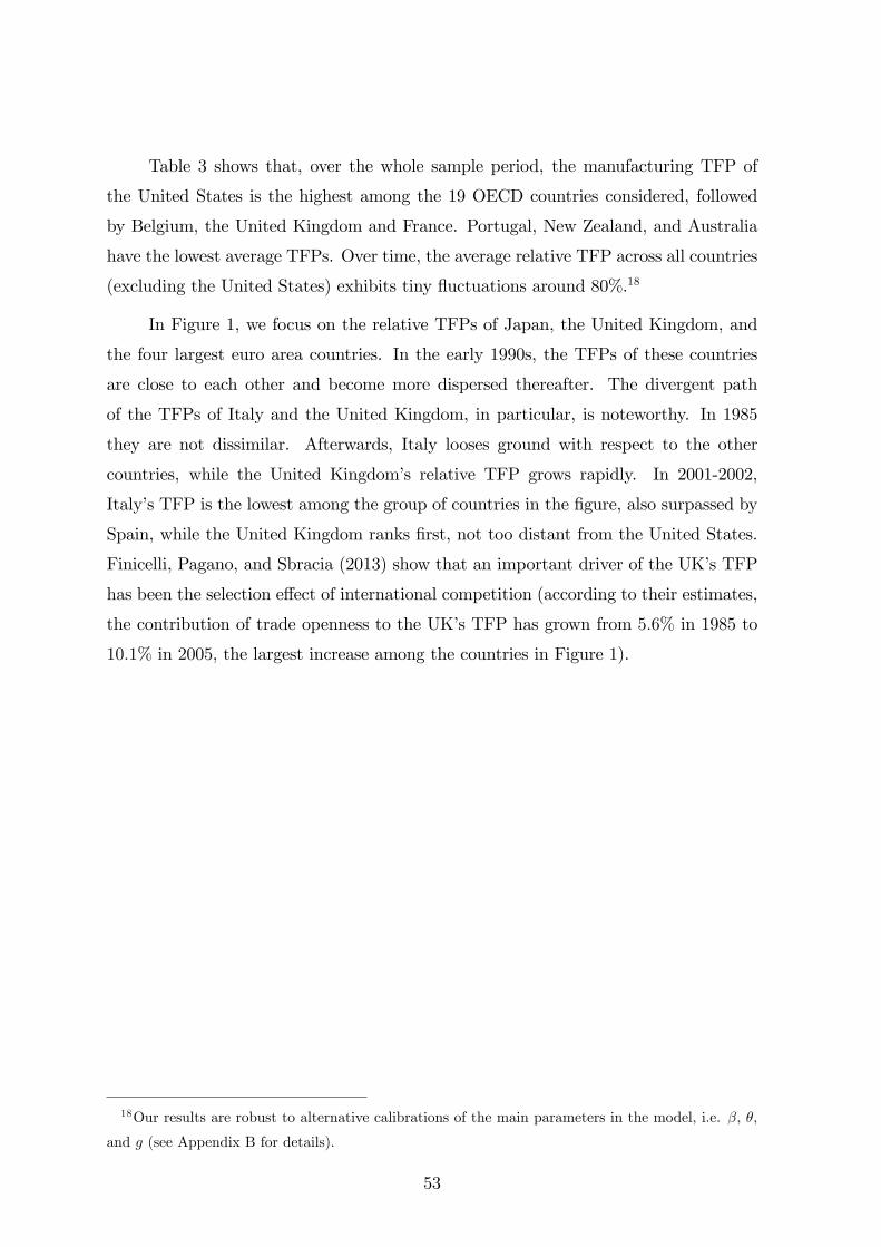
(2.) 4. Results 52
(2.) 5. A case study: Italy vs. the United States 59
(2.) 6. Conclusion 61
Appendix A. Data 63
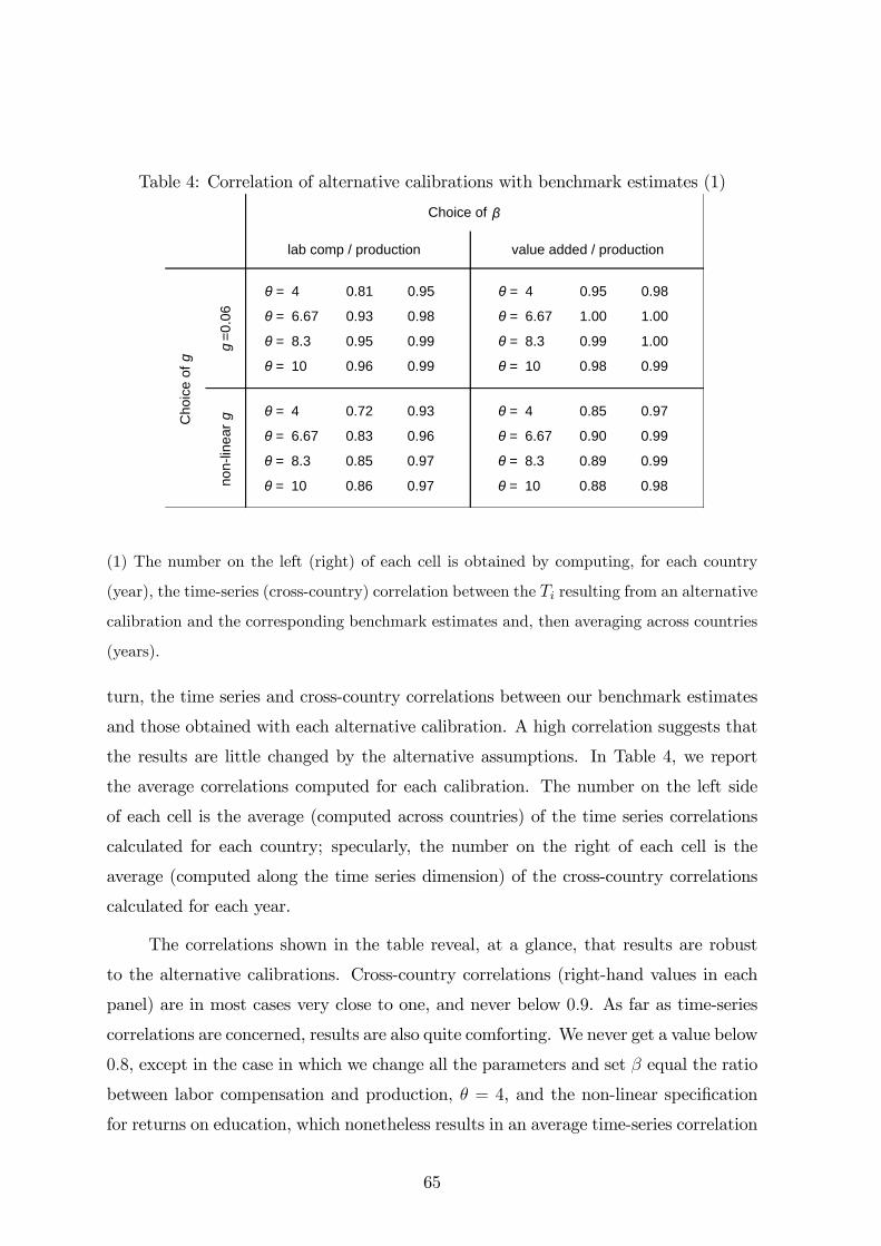
Appendix B. Sensitivity analysis 64
Appendix C. The model with physical capital 66
IV
Chapter 3. Exchange Rates in a General Equilibrium Model of Tradewithout Money (with V. Di Nino and B. Eichengreen) 69
(3.) 1. Introduction 71
(3.) 2. The model 75
(3.) 2.1. Closed economy 75
(3.) 2.2. Open economy 77
(3.) 3. Changes in exchange rates 82
(3.) 4. Conclusion 86
Appendix A. The closed economy model 88
Appendix B. The open economymodel 90
Appendix C. Proof for Proposition 1 93
Appendix D. Proof for Proposition 2 94
Appendix E. Proof for Proposition 3 97
Chapter 4. Summary and conclusions 99
References 105
V
VI
Introduction
The importance of cross-country di¤erences in industry e¢ ciencies for interna-
tional trade �ows has been recognized in the economic literature since at least the
work of David Ricardo (1817).1 During the XIX century, Ricardo�s famous example �
which explained how England and Portugal could both bene�t from international trade
by exploiting their comparative advantage in making clothes and wine � was gradu-
ally turned into a formal model. Solving for equilibrium quantities and relative prices,
however, was quite tedious even in the case of a world economy with only few coun-
tries and goods, making it di¢ cult to derive general comparative statics results (Eaton
and Kortum, 2012). Moreover, the enduring lack of a treatable general-equilibrium
model prevented to use Ricardian trade theory for empirical applications as well as for
answering meaningful theoretical questions.
In recent years, instead, the theory of comparative advantage has experienced a
revival, favored by two major breakthroughs.
First, Dornbusch, Fischer and Samuelson (1977) showed that, by considering a
continuum of tradeable goods, the model simpli�ed neatly with respect to the discrete
many-commodity case. In fact, one could represent industry e¢ ciencies (of a country
relative to another one) with a mathematical function and then use the tools of calculus
to derive equilibrium quantities and relative prices. This model simpli�ed the task of
deriving the full competitive equilibrium, but could handle only the case of a world
economy with just two countries.
Second, after further 25 years, it was �nally laid out the full-�edged many-country
many-good model. This happened when Eaton and Kortum (2002) focused on speci�c
functions, namely cumulative distribution functions, to represent industry e¢ ciencies
in di¤erent countries. In particular, they assumed that the e¢ ciencies of the various
industries in each country could be described by a Fréchet cumulative distribution
1Chipman (1965) provides a famous survey and a discussion of the contribution of Ricardo (1817) to
the so-called "classical" theory of international trade, comparing it to the previous studies of Torrens
(1808 and 1815). See also Seligman (1903) for an early comparison of the contributions of Ricardo
and Torrens.
1
function.2 By adding an hypothesis about the strength of the cross-country correlations
of industry e¢ ciencies, their model exploited the language of probability to obtain
equilibrium quantities and relative prices.3
In this model, the full general equilibrium is the solution of a system of equa-
tions, with parameters that depend on consumer preferences, labor endowments, trade
barriers and the probability distributions representing industry e¢ ciencies. Due to the
presence of non-linearities, the system does not have a closed-form solution. Never-
theless, results by Alvarez and Lucas (2007) grant that a solution of the system exists
and that it is unique. In addition, the parameters can all be estimated or calibrated,
including those of the probability distributions representing technologies. The unique
equilibrium quantities and relative prices can then easily be obtained by resorting to
standard numerical methods to solve the system.
Thus, the lack of a closed form solution does not prevent to quantify the model
and perform counterfactual simulations. In the last few years, in fact, several exercises
have been performed and various empirical questions have been explored, including the
quanti�cation of the welfare e¤ects of changes in trade barriers, the impact of an im-
provement in domestic and foreign technologies, the importance of capital endowment
and technology for shaping industry specialization, and the size of the change in factor
costs needed to balance current accounts across all countries.4
In this thesis, we take an alternative route and explore the possibility of using
the Ricardian model in order to tackle a set of theoretical questions. Speci�cally,
we consider variants and extensions of the Eaton-Kortum model, in order to analyze
di¤erent, albeit strictly related, issues, concerning the sources of the welfare gains from
2The Fréchet distribution is a heavy-tailed distribution that, together with the Pareto and Lognor-
mal distributions, is commonly used to model e¢ ciencies at the industry or the �rm level (see Eaton
and Kortum, 2002).
3The most convenient assumption about the strength of the cross-country correlations of industry
e¢ ciencies is the hypothesis of independence, which is the one adopted in the basic model. This
restrictive assumption, however, can be easily relaxed in favor of positive or negative correlation (see
Eaton and Kortum, 2002, and Finicelli, Pagano and Sbracia, 2013).
4See, for example, Eaton and Kortum (2002), Shikher (2011), Dekle, Eaton and Kortum. (2007),
and Waugh (2010). For a survey, see also Eaton and Kortum (2012).
2
trade, the e¤ects of trade openness on total factor productivity, and the role of nominal
exchange rates.
The �rst chapter, written with Stefano Bolatto (University of Bologna), relaxes
the assumption of Fréchet-distributed e¢ ciencies, extending the Eaton-Kortum model
to general technologies represented by generic distributions of industry e¢ ciencies. For
this very general Ricardian framework, we show that the welfare gains from trade can
always be decomposed into a selection e¤ect and a reallocation e¤ect. The former is
the e¤ect on average e¢ ciency of the mechanism of selection of industries that, thanks
to su¢ ciently low marginal costs of production relative to foreign industries, make
only some industries survive to international competition. The latter e¤ect, instead, is
related to the rise in the weight of exporting industries in domestic production, which is
due to the reallocation of workers away from the less-e¢ cient non-exporting industries
to the industries that start servicing the foreign market.
Although the model provides very precise theoretical de�nitions for both e¤ects,
their analytical expression is, in general, too cumbersome to be used for empirical
purposes. In particular, with N countries, one should compute the distributions of
the e¢ ciencies for the industries that export in each of the N � 1 foreign countries,the distributions of the e¢ ciencies for the industries that export in all the possible
N (N � 1) =2 couples of countries, etc.. In most applications, this calculation wouldrequire computing several billions of distributions of e¢ ciencies. For example, in the
46-country application that we consider in the chapter, one would have to compute
more than 35,000 billions of di¤erent distributions.
By contrast, this decomposition simpli�es dramatically if we impose that indus-
try e¢ ciencies are Fréchet distributed. This assumption makes our general Ricardian
model return to the original Eaton-Kortum model. Under this assumption, we derive
exact model-based measures of these two e¤ects, which can be easily quanti�ed using
data on trade �ows and domestic production.
A quanti�cation for a sample of 46 advanced and developing economies in the
years 2000 and 2005 shows that the selection e¤ect is, on average, somewhat more
important than the reallocation e¤ect (accounting for about 60% of the gains from
trade). In particular, the former e¤ect is dominant for large countries: only in the
United States and Japan, among the advanced economies, and in Brazil, Russia, India,
3
and China, among the developing countries, does the share of gains pertaining to the
selection e¤ect exceeds 80%. However, for small open economies such as Denmark,
Ireland, the Netherlands, Singapore, Thailand, and Vietnam, it is the reallocation
e¤ect that dominates, as it is responsible for over 70% of the gains.
The second chapter, written with Andrea Finicelli (Bank of Italy) and Patrizio
Pagano (Bank of Italy), focuses on the e¤ects of trade openness on total factor pro-
ductivity (TFP), which is closely related to that of the welfare gains from trade. The
relationship between welfare and TFP stems from the fact that, at a global level, the
growth in world-wide aggregate TFP induced by international trade is the basic source
of the welfare gains for all countries. In other words, countries bene�t from the fact
that, after opening to trade, specialization makes the world to produce more of each
good. This additional production comes from the selection and the reallocation e¤ect
discussed in Chapter 1. In particular, the selection e¤ect is such that only a set of
domestic industries survives the competition from foreign industries and, therefore,
the average of the e¢ ciencies across domestic industries, on which Chapter 2 focuses,
changes due to international trade.
We �rst prove formally that the average productivity across "active" domestic
industry is a good proxy for the aggregate TFP of both the closed and the open
economy.5 We then take the former as our measure of productivity, which we dub
trade-revealed TFP, and introduce a novel methodology to measure the relative TFP
of the tradeable-goods sector of various countries. This new approach is based on
the theoretical relationship between trade openness and TFP in the Eaton-Kortum
model. The logic of our methodology is to use a structural model and measure TFP
not from its "primitive" (which is the aggregate production function in the standard
development-accounting approach), but from its observed implications. Speci�cally,
our trade-revealed TFP is the average productivity that best �ts data on trade, pro-
duction and factor costs.
5With the term average productivity we refer to the �rst moment of the e¢ ciency distribution of the
active industries. In the closed economy, this is simply the �rst moment of the Fréchet distribution,
which describes the e¢ ciencies of all the industries. In the open economy, average productivity of the
industries that survive international competition is the same as the average productivity of the closed
economy, augmented by a measure of trade openness.
4
The main advantage of our methodology is that TFP is no longer a mere resid-
ual. Moreover, our measures turn out to be easier to compute than in the standard
development-accounting approach.
Using annual data from 1985 to 2002, we thus estimate TFP levels, relative to the
United States, of 19 OECD countries. Results show a close resemblance between the
trade-revealed TFP and the TFP derived from the standard approach. In addition, our
measures do not yield common "anomalies," such as the higher TFP of Italy relative
to the United States.
The third chapter, written with Virginia Di Nino (Bank of Italy) and Barry
Eichengreen (University of California, Berkeley), builds on the previous two, which fo-
cused on welfare and productivity, and studies these variables (together with GDP and
employment) in a more general setting, in which the Eaton-Kortum model is extended
to incorporate also the non-tradeable-goods sector. The main purpose of Chapter 3 is
to analyze the domestic and international e¤ects on welfare, productivity, GDP and
employment of "misaligned currencies," i.e. of currencies that are either undervalued
(say "excessively competitive") or overvalued ("scarcely competitive") with respect to
their long-run equilibrium level.
The main challenge that we have to face in order to examine this question is how
to introduce a nominal variable like the exchange rate into a model of real consump-
tion and production decisions, in which there is no money. We do so by building on
the insight of Keynes (1931) that the combination of an import tari¤ and an export
subsidy � which are two parameters in our model � is isomorphic to an exchange
rate depreciation. By mimicking changes in exchange rates with changes in the model
parameters, we can demonstrate a series of classical results and conjectures in a very
general framework with a multiplicity of countries, tradeable goods and non-tradeable
goods.
This chapter obtains three main theoretical results:
� First, we show that a depreciation has no real e¤ects with �exible wages. Thedecline in marginal costs due to the depreciation is, in fact, completely o¤set
by a proportional rise in relative wages, as it is to be expected in a frictionless
economy.
5
� Second, by assuming sticky wages, we are able to prove that an undervaluedcurrency causes involuntary unemployment abroad, while at home it determines
ine¢ ciently high employment in the high-productivity export sector. This em-
ployment misallocation raises real GDP but lowers welfare, as real wages are too
low.
� Finally, we show that if the currency is overvalued, then there exists an appro-priate depreciation that restores the relative prices of the long-run competitive
equilibrium across countries, with welfare-enhancing e¤ects � a result that pro-
vides the �rst formal proof of Friedman�s conjecture (1953).6
Thus, our results show formally, in a general equilibrium framework, the domestic
and international e¤ects of a nominal depreciation of a currency (and, by the same
token, of a nominal appreciation).
In particular, if wages are sticky and the depreciation makes the currency under-
valued (i.e. relative wages become lower than their long-run value), then workers shift
from the non-tradeable-goods to the tradeable-goods sector. The relative size of latter,
however, becomes ine¢ ciently large and, although the domestic economy preserves full
employment and real GDP rises, welfare declines. Moreover, undervaluation causes
involuntary unemployment abroad, because foreign workers are displaced by the "ex-
cessive competitiveness" of the domestic economy and only some of them, but not all,
�nd a job in the non-tradeable-goods sectors.
On the other hand, if the depreciation takes place at a time in which the currency
is overvalued (i.e. relative wages are higher than in the long-run equilibrium), then
it facilitates the return of the economy to its competitive equilibrium, with a small
in�ationary impact and welfare-enhancing e¤ects. The increase in consumer prices is
"small" because, following the depreciation, domestic wages do not rise and, impor-
tantly, would not rise even if they were perfectly �exible. If domestic wages (relative
to foreign wages) were higher than what they should have been in the long-run com-
petitive equilibrium, in fact, an appropriate currency depreciation can bring them to
6Friedman (1953, p. 173) conjectured that, in case of misalignments in nominal wages across
countries, one could quickly restore the long-run competitive equilibrium just by allowing the exchange
rate to properly adjust, rather than by changing the entire internal wage-price structure. In other
words, exchange rates could solve the enormous coordination problem of wage and price setters.
6
their equilibrium level. Thus, depreciation can substitute for the adjustment of relative
wages, con�rming Friedman�s (1953) intuition.
The fourth chapter summarizes the most important �ndings, draws the main
conclusions and, together with a discussion of some limits of the various models pre-
sented in the thesis, o¤ers some related suggestions for future research.
7
8
CHAPTER 1
Deconstructing the Gains from Trade:Selection of Industries vs. Reallocation of Workers
9
10
1 Introduction
In a very in�uential paper, Arkolakis, Costinot, and Rodríguez-Clare (2012) have shown
that the welfare gains from trade implied by a very large class of models depend on
only two su¢ cient statistics: (i) the share of expenditure on domestic goods (which is
often called "domestic trade share"); and (ii) the elasticity of imports with respect to
variable trade costs ("trade elasticity"). This result is remarkable because it applies
to frameworks as di¤erent as the simple Armington model, in which goods are di¤er-
entiated by country of origin; the Ricardian model with heterogeneous industries and
Fréchet-distributed e¢ ciencies of Eaton and Kortum (2002); the monopolistic compe-
tition model of Krugman (1980); as well as variants of the monopolistic competition
model of Melitz (2003), with heterogeneous �rms and Pareto-distributed e¢ ciencies
(such as those developed by Chaney, 2008, and Eaton, Kortum, and Kramarz, 2011).
Given their importance for empirical studies, these models are now commonly referred
to as "quantitative trade models."
Following this result, the literature appears to be taking two main directions. One
analyzes how the measurement of the gains from trade changes when some assumptions
of quantitative trade models are relaxed (see Arkolakis, Costinot, Donaldson, and
Rodríguez-Clare, 2015, and Melitz and Redding, 2014 and 2015). The other focuses on
the empirical implications of the result. In particular, it is now clear that the various
models have di¤erent implications for the estimated value of the trade elasticity, so
that even though the analytical formulation of the gains from trade is the same, the
resulting quanti�cation still di¤ers across models (Simonovska and Waugh, 2014a).
In this chapter we explore a di¤erent route, by focusing on the sources of the
welfare gains of the open economy with respect to the autarky economy as well as
on their quanti�cation. In particular, we study whether quantitative trade models
allow us to measure not only the overall welfare gains, but also the contribution of
the di¤erent sources � a key issue in both the theoretical and the empirical literature
in international trade. Answering this question, however, is in general very di¢ cult,
because di¤erent quantitative models entail di¤erent predictions on the sources of the
welfare gains. For example, the gains from consuming a greater variety of goods are
key in Armington and monopolistic competition models, but are absent in Ricardian
11
models. Given these sharp di¤erences, we analyze this question for one speci�c family
of models and investigate whether belonging to the class of quantitative trade models
facilitates the measurement of the contribution of the di¤erent sources.
The family on which we focus is the Ricardian model with many countries and
goods, CES preferences, and general distributions of industry e¢ ciencies. Thus, with
respect to Arkolakis, Costinot, and Rodríguez-Clare (2012), although we restrict the
attention to only one family of models, we extend the scope of the analysis by providing
general results for Ricardian models in which industry e¢ ciencies follow a generic
distribution, and not necessarily a Fréchet.
For this general family of models, we show that the welfare gains of the open
economy with respect to the autarky economy can always be decomposed into two dis-
tinct sources: a selection and a reallocation e¤ect. The former is the e¤ect on average
e¢ ciency of the selection of domestic industries that, thanks to their su¢ ciently low
marginal costs of production relative to foreign industries, survive international compe-
tition. Such average e¢ ciency is computed by considering, for the sole industries that
survive international competition, the same relative weights in domestic production as
the autarky economy. The latter e¤ect, instead, is related to the rise in the weight
in domestic production of the exporting industries, which is due to the reallocation
of workers away from the less-e¢ cient non-exporting industries to the industries that
start servicing the foreign market.
While the model provides very precise theoretical de�nitions for both e¤ects,
their analytical expression is, in general, too cumbersome to be used for empirical
purposes. In most applications, in fact, it would require computing several billions
of distributions of e¢ ciencies. By contrast, this decomposition simpli�es dramatically
if we impose that industry e¢ ciencies are Fréchet distributed � the assumption that
makes our Ricardian model belong to the class of quantitative trade models. Under
this assumption, we can derive exact model-based measures of these two e¤ects, which
can be quanti�ed using only data on trade �ows and domestic production.
The Fréchet assumption entails this simpli�cation for the following reasons. First,
it allows us to easily quantify the overall gains from trade, as in Arkolakis, Costinot,
and Rodríguez-Clare (2012). Second, it implies that the selection e¤ect is a measurable
share of the overall gains from trade, making it possible to easily obtain the contribu-
12
tion to welfare of this e¤ect. Third, as a consequence, the reallocation e¤ect (whose
quanti�cation is, in the general case, extremely di¢ cult) can be calculated simply as
the complement of the selection e¤ect. Therefore, a key insight of our analysis is that
quantitative trade models may be useful not only to assess the overall welfare gains,
but also to properly measure their sources.
Using the Fréchet assumption, we also demonstrate that, when the gains from
trade are small and there are still few exporters in the domestic economy, the largest
share of the welfare gains is due to the selection e¤ect. As the export sector grows
and the gains from trade increase, the importance of the reallocation e¤ect also rises.
Because the contribution of the reallocation e¤ect grows with the size of the overall
gains from trade, it follows that the factors a¤ecting the former are exactly the same
factors a¤ecting the latter. In particular, both the welfare gains and the contribution
of the reallocation e¤ect are higher for small, open and very productive economies,
located near to markets that are large, rich, and less productive and, therefore, easier
to penetrate. Another interesting feature of our result is that the speci�c value of the
trade elasticity, which is key to determine the overall welfare gains, does not a¤ect the
shares of the gains pertaining to the selection and the reallocation e¤ect, making their
measurement even more straightforward and robust than that of the welfare gains.
A quanti�cation for a sample of 46 advanced and developing economies in the
years 2000 and 2005 shows that the selection e¤ect is, on average, somewhat more
important than the reallocation e¤ect (accounting for about 60% of the gains from
trade). In particular, the selection e¤ect is dominant for large countries: only in
the United States and Japan, among the advanced economies, and in Brazil, Russia,
India, and China, among the developing countries, does the share of gains pertaining
to the selection e¤ect exceeds 80 percent. However, for small open economies such
as Denmark, Ireland, the Netherlands, Singapore, Thailand, and Vietnam, it is the
reallocation e¤ect that is dominant, as it is responsible for over 70 percent of the gains.
These �ndings have important policy implications. Suppose that the export sector
is less similar to other sectors of the economy in terms of, for example, skills that are
required to workers, as documented by the empirical literature.1 This feature of the
1Bernard, Jensen, Redding and Schott (2007) show, in fact, that exporting �rms are more skill
intensive than their domestic competitors.
13
export sector could make the resource reallocation from other industries slower or more
di¢ cult. In this case, our theoretical and empirical results suggest that, in the initial
stages of trade liberalization (i.e. when trade barriers are still high), these frictions do
not prevent to reap the bene�ts from trade, because most of the gains obtain from the
selection e¤ect, that is from the closure of less e¢ cient industries and the reallocation of
workers across all the surviving industries, which are mostly non-exporters. Similarly,
large countries can expect to enjoy welfare gains almost in full, even in the hypothesis
of a cumbersome reallocation to the export sector, thanks to the considerable size of
their non-exporting industries. On the other hand, reallocation of workers to the export
sector is crucial in small open economies. Therefore, to fully bene�t from trade, these
countries must be ready to favor the resource reallocation to this sector, in particular
by enhancing education and training for unskilled workers.
Our chapter is related to several strands of the literature. Many recent empir-
ical and theoretical studies have focused on one speci�c source of the welfare gains,
that is aggregate productivity. An early example is Pavcnik (2002), who estimates
productivity improvements in Chile using �rm-level data. This study con�rms the im-
portance of the mechanisms described in this chapter, as it �nds that the exit of plants
and the reshu ing of resources from less e¢ cient to more e¢ cient producers are the
main sources of the productivity gains. Many other papers, instead, have focused on
model-based measures of the "productivity gains from trade," computed as increases
in the average e¢ ciency.2 To better grasp the link between these papers and our own,
it is worth recalling that, in the Ricardian model, the growth in world-wide aggregate
productivity induced by international trade is the basic source of the welfare gains for
all countries. In other words, countries bene�t from the fact that, by specializing in
the production of the goods for which they have a comparative advantage, the world
production of the optimal consumption bundle increases. Thus, our chapter sheds light
on how each individual country, through the mechanisms of selection and reallocation
induced by trade liberalization, contributes to the improvement of the world-wide ag-
gregate productivity and reaps the bene�ts of international trade for its own welfare.
2See, for example, Bernard, Eaton, Jensen, and Kortum (2003), Costinot, Donaldson, and Ko-
munjer (2012), Bolatto (2013), Finicelli, Pagano and Sbracia (2013 and 2015), and Levchenko and
Zhang (2015).
14
Another related strand of the literature is the wave of papers focusing on empirical
estimates of the gains from trade, such as Feenstra (1994 and 2010), Broda and Wein-
stein (2006), Goldberg, Khandelwal, Pavcnik, and Topalova (2009), and many others.
These papers use di¤erent econometric techniques to quantify either the contribution
of speci�c sources of gains (usually those from consuming new varieties) or the size of
the overall welfare gains. Our approach, instead, grounded on the derivation of model-
based measures of the welfare gains, follows more closely the one of Eaton and Kortum
(2002), Alvarez and Lucas (2007), Arkolakis, Demidova, Klenow, and Rodríguez-Clare
(2008), Chor (2010), Arkolakis, Costinot, and Rodríguez-Clare (2012), and Ravikumar
and Waugh (2015). Unlike those papers, however, we are also able to quantify the
contribution of the di¤erent sources of gains.3
Our chapter complements Finicelli, Pagano and Sbracia (2013), who focus on the
average e¢ ciency of domestic industries (instead of welfare), which is a¤ected only by
the selection e¤ect. In an open economy, welfare di¤ers from the average e¢ ciency
of domestic industries, because it depends not only on the e¢ ciencies of domestic
industries (which determine the price of domestically-produced goods), but also on the
e¢ ciencies of foreign industries (which determine import prices). Thus, welfare and
the average e¢ ciency of domestic industries are distinct concepts. In this chapter we
show that the balanced-trade condition allows us to derive the welfare contribution of
imports by using exports; this makes it possible to compute such contribution starting
from the e¢ ciency distribution of domestic industries. By using this technique, we
can decompose the welfare gains into the selection and the reallocation e¤ect discussed
above. As we show, the selection e¤ect turns out to be related to the average price of
domestically-produced goods and the reallocation e¤ect to the average price of imported
goods.4
3A close relative of our study is also the paper by Demidova and Rodríguez-Clare (2009), who
decompose the welfare gains from trade of a small open economy under monopolistic competition
into four terms: productivity, terms of trade, number of varieties, and curvature (i.e. the degree of
heterogeneity across varieties). Here, instead, we consider a general equilibrium model with perfect
competition and, most importantly, we derive a quanti�able expression of the two sources that, in our
Ricardian framework, provide the welfare gains.
4It is worth noting that Finicelli, Pagano and Sbracia (2013, pg. 100) also mention a "market-share
reallocation e¤ect" but, in that paper, that is the e¤ect of reallocation on labor productivity and not
on welfare. Unlike their counterparts on welfare, the selection and the reallocation e¤ect on labor
15
The rest of the chapter is organized as follows. Section 2 describes the model,
which extends Eaton and Kortum (2002) to general distributions of industry e¢ cien-
cies. Section 3 shows that the welfare gains induced by international trade can be
decomposed into two distinct e¤ects, related to the selection of industries and the
reallocation of workers. Section 4 introduces the assumption of Fréchet-distributed
industry e¢ ciencies, shows that the analytical expressions of the two e¤ects simplify,
and quanti�es them for a sample of countries and years. Section 5 draws the main
conclusions.
2 The model
We consider a continuum of tradable goods, indexed by j 2 [0;+1), that can poten-tially be produced in any of the N countries of the world economy. Each good j can be
produced in country i with an e¢ ciency zi (j) that, in turn, is de�ned as the amount of
output that can be produced with one unit of input � where both output and input
are measured in units of constant quality. Any country has a �xed labor endowment Li.
Inputs include labor as well as a bundle of intermediates goods, which comprises the
full set of tradable goods j.5 Technology is described by a Cobb-Douglas production
function with constant returns to scale, in which labor has a constant share � � 1 forall industries and countries; namely:
qi (j) = zi (j)L�i (j) I
1��i (j) , (1)
where qi (j) is the quantity of output j in country i, Li (j) is the number of workers,
and Ii (j) is the quantity of the bundle of intermediate goods.
Consumer preferences are the same across countries. The representative consumer
in country i purchases individual goods in amounts ci(j) in order to maximize a CES
utility function:
Ui =hR[ci(j)]
��1� dj
i ���1
,
productivity are analytically indistinguishable and hard to quantify, even in the two-country case. On
the contrary, the selection and the reallocation e¤ect on welfare are analytically distinct and easily
measurable.
5We can ignore physical capital in the production function because the model is static and, then,
intermediate inputs play a very similar role.
16
where � > 0 is the elasticity of substitution. While the model allows us to deal with
both inelastic (� � 1) and elastic demand (� > 1), we will focus on the latter case,
because the goods that we consider are all tradable and, in this setting, the typical
calibration is � > 1.6
Consumers maximize their utility function subject to a standard budget con-
straint. Because we assume that trade is balanced in the open economy, income avail-
able for consumption is Yi = wiLi, where wi is the (nominal) wage.
International trade is constrained by barriers, which are modeled using the stan-
dard assumption of iceberg costs; i.e., delivering one unit of a good from country i to
country n requires shipping dni units, with dni > 1 for i 6= n and dii = 1 for any i. Byarbitrage, trade barriers obey the triangle inequality, so that dni � dnk � dki for any n,i and k.
Perfect competition implies that the price of one unit of good j produced by
country n and delivered to country i is:
pin (j) =cndinzn (j)
,
where cn = w�np1��n is the cost of one unit of input in the source country n, with pn
being the unit price of the optimal bundle of intermediate goods, which is the same as
the unit price of the optimal bundle of �nal goods (see equation (3) below). In other
words, we assume (as Eaton and Kortum, 2002) that producers combine intermediate
goods using the same CES aggregator that consumers use to combine �nal goods.
Consumers purchase each good from the country that can supply it at the lowest
price; therefore, the price of good j in country i is:
pi (j) = minn
�cndinzn (j)
�.
We assume that, in each country i, industry e¢ ciencies zi(j) are the realiza-
tions of a random variable Zi, with a country-speci�c cumulative distribution function
(c.d.f.) Fi. Because the zi (j) represent industry e¢ ciencies and there is a continuum
of goods, it is natural to assume that Zi is non-negative and absolutely continuous
6For an extension of the model that encompasses both tradable and non-tradable goods, see Di
Nino, Eichengreen, and Sbracia (2013).
17
for each country i. These are the only conditions that we impose, in this and in the
following section, on the Zi�s (in Section 4, instead, we assume that the Zi are Fréchet
distributed). As the expert reader may have noticed, we do not impose the standard
restriction that the Zi are mutually independent across countries, but we allow for
dependent (correlated) variables.
The continuum-of-goods assumption and the conventional application of the law
of large numbers imply that the share of goods for which country i�s e¢ ciency is below
any real number z is the probability Pr (Zi < z) = Fi (z). It is worth noting that,
in the autarky economy, all goods are made at home and, then, Zi is the e¢ ciency
distribution of the closed economy.
Given the cost of inputs, the distribution of industry e¢ ciencies translates into a
distribution of good prices. More formally, let us denote with Pi the random variable
that describes the distribution of good prices in country i; this random variable is
de�ned as:
Pi = minn
�cndinZn
�=
�maxn
�Zncndin
���1. (2)
The price index in country i, pi, computed using the correct CES aggregator, is simply
the moment of order 1� � of the random variable Pi, at the 1= (1� �) power; that is:
pi =�E�P 1��i
��1=(1��). (3)
After a simple manipulation of equations (2) and (3), we obtain:
pi = ci ��E�M��1i
��1=(1��),
where Mi = maxn
�cicn
Zndin
�, (4)
that leads to the real wage, which measures welfare:7
wipi=�E�M��1i
��1=�(��1). (5)
The welfare gains from trade can be obtained by comparing the real wage of the
open and the closed economy, where the latter can be obtained from the former, letting
7Recall that, in the competitive equilibrium of both the open and the closed economy, welfare is
Ui = wiLi=pi, where Li is exogenous.
18
din ! +1 for i 6= n (using equations (4) and (5)). In this case, we have Mi ! Zi and
the real wage is�E�Z��1i
��1=�(��1). Hence, the gain from trade for country i is:
gi =
"E�M��1i
�E�Z��1i
� #1=�(��1) . (6)
Equation (6) shows that welfare gains arise from the transformation, that occurs in
the open economy, of the "source of the production e¢ ciencies" (e¢ ciencies that, in
turn, determine good prices) from Zi toMi. Note, in particular, that the latter random
variable is a maximum between a set of random variables that includes also Zi. Because
the maximum of a set of random variables �rst-order stochastically dominates any
variable included in the set, thenMi � Zi, so that gi � 1.8 In other words, the real wageis higher in the open economy. Thus, the result that trade is welfare improving is here
proven using the language of probability, rather than the tools of general equilibrium.9
3 Welfare decomposition
Let us now focus on how labor units are reallocated after opening to trade. To fos-
ter intuition, we start by considering the case of two countries, say i and n, before
generalizing the result to N countries.
3.1 A 2-country example
The �rst-order conditions (FOCs) of the consumer�s problem imply that the demand
for good j in country i is:
ci (j) =
�pi (j)
pi
���� Ui , (7)
where Ui = wiLi=pi is the level of utility achieved by country i.
8We remind the reader that the random variable X �rst-order stochastically dominates the random
variable Y , and we write X � Y , if and only if FX (z) � FY (z) for any z 2 R, where FX and FY are
the c.d.f. of, respectively, X and Y . If this condition holds, then E�Xk�� E
�Y k�, for any k > 0.
9The �nding that gi � 1 for any i, proven using basic probability theory, generalizes a result of
Finicelli, Pagano, and Sbracia (2013), extending it to a framework in which there are also intermediate
goods.
19
The FOCs of the producer�s problem, on the other hand, imply that the quan-
tities of labor and intermediate goods used to produce good j in country i are chosen
according to the following proportions:
Ii (j) =1� ��
wipiLi (j) . (8)
By aggregating across industries both sides of equation (8), we �nd that the overall
amount of intermediate goods used in country i is Ii =1���� (wi=pi) � Li.
The assumption that intermediate goods are combined using the same CES ag-
gregator used to combine �nal goods implies that, for any country i, the demand for
j as intermediate good, mi (j), is proportional to the demand as consumption good,
ci (j); that is: ci (j) =Ui = mi (j) =Ii. Because Ii=Ui = (1� �) =�, it follows that, incountry i, the demand for good j as an intermediate input is mi (j) = (1� �) �ci (j) =�.Hence, in any country i, the overall demand for good j is ci (j) =�.
In the two-country model that we are examining, each good can either be pro-
duced abroad and imported at home; or be produced at home and sold only in the
domestic market; or be produced at home and sold both in the domestic and the
foreign market. Therefore, the resource constraint for country i requires that:
qi (j) =
8>><>>:0 if j 2 Oi;z
1�ci (j) if j 2 Oi;d
1�[ci (j) + cn (j) dni] if j 2 Oni;e
, (9)
for any j, where Oi;z denotes the set of "zombie" industries of country i, i.e. those
industries that shut down right after trade liberalization;10 Oi;d is the set of industries
that sell their goods only on the domestic market; and Oni;e is the set of industries
that sell both at home and in country n:11 By construction, the sets Oi;z, Oi;d, and
Oni;e form a partition of the set of tradable goods; hence, the intersection between any
subset of them is empty and their union spans the whole set of tradable goods. The
10We borrow the terminology "zombie industries" from Caballero, Hoshi, and Kashyap (2008), who
use it to refer to industries that are kept alive only by misdirected or subsidized bank lending. In the
context of our model, instead, these industries would be kept alive by trade protectionist policies.
11In the two-country model, these sets are de�ned as follows: Oi;z =nj : zi(j)ci
> zn(j)cndin
o, Oi;d =n
j : zn(j)cndin� zi(j)
ci< zn(j)dni
cn
o, and Oni;e =
nj : zi(j)ci
� zn(j)dnicn
o.
20
set Oi;o � Oi;d [ Oni;e, on the other hand, includes the sole industries that surviveinternational competition.12
By plugging equations (1) and (7) into equation (9) (using also equation (8)),
and solving the resource constraint for the number of workers in industry j, we obtain:
Li (j) =
8>>><>>>:0 if j 2 Oi;z
z��1i (j) ��wipi
��(1��)Li if j 2 Oi;d
z��1i (j) ��wipi
��(1��)Li � (1 + kni) if j 2 Oni;e
, (10)
where:
kni =wnLnwiLi
�pidnipn
�1��. (11)
The term kni measures the rise in the weight of the exporting relative to non-exporting
industries. It is related to the demand that comes from country n, since it depends
positively on the size of this country in terms of relative GDP, and negatively on the
iceberg cost between countries i and n, and their relative price levels.
In the autarky economy, Oi;z = Oni;e = ? and the resource constraint returns, for
any good j, Li (j) = z��1i (j) � (wi=pi)�(1��) Li. Let us consider, then, how labor is re-allocated after trade liberalization. With respect to the autarky economy, in the open
economy the number of workers in the zombie industries goes to zero. The number of
workers in the industries that produce goods that are sold only domestically declines
(provided that � > 1), because these industries face a tougher competition, due to the
fact that imported goods are cheaper than those that were made at home under the
autarky regime.13 The number of workers in the exporting industries rises, absorb-
ing all the workers "in excess" from the other domestic industries. More speci�cally,
these industries sell less in the domestic market (as international competition brings
in cheaper imported goods), so they would need less workers to serve this market, but
foreign demand allows them not only to keep their workers, but also to hire new ones
12The term cn (j) dni=� in equation (9) represents the foreign demand that bene�ts only the export-
ing industries. In particular, the representative consumer of country n demands the quantity cn (j) =�,
but iceberg costs imply that dni units must be shipped from country i to deliver one unit of good to
country n. Thus, the overall quantity produced to serve the latter market is cn (j) dni=�.
13If � < 1 (� = 1), industries producing goods that are sold only at home would employ more (the
same number of) workers.
21
in order to produce more goods to be sold abroad.14
Notice that, in any industry, the number of workers is proportional to the e¢ -
ciency of this industry, at the � � 1 power (i.e. to z��1i (j)). By aggregating across
industries both sides of equation (10), we obtain:
Li =
�wipi
��(1��)Li �
"Zj2Oi;d
z��1i (j) dj + (1 + kni)
Zj2Oni;e
z��1i (j) dj
#�wipi
��(��1)=
Zj2Oi;o
z��1i (j) dj + kni
Zj2Oni;e
z��1i (j) dj ,
from which we can derive the following decomposition of the real wage (which is proven
in Appendix A for the general N -country case):15
wipi=
24�i;o � E �Z��1i;o
�| {z }selection
+ �i;e � kni � E�Z��1i;e;n
�| {z }reallocation
351=�(��1) , (12)
where �i;o is the probability that an industry of country i survives international com-
petition; �i;e is the probability that it is also an exporter (with �i;e � �i;o);16 Zi;o is therandom variable that describes the e¢ ciencies of the surviving industries; and Zi;e;n
describes the e¢ ciencies of the industries that export in country n.
Equation (12) shows � together with equation (10), from which it is derived �
the two sources of the welfare gains of this model. The �rst one comes from impact of
the selection of industries due to international competition, that transforms the average
e¢ ciency of the economy from E(Z��1i ) into E(Z��1i;o ). The second one comes from the
reallocation of workers to the exporting industries, which provides a contribution to
welfare that is separate and additional to the previous one (measured by the second
term inside the square brackets on the right-hand side of (12)).17 This contribution
14For j 2 Oni;e, the two terms of equation (10) represent exactly these factors: the number of workersin the exporting industry that serve the domestic market (which declines after trade liberalization)
and the number of workers hired to start servicing the foreign market.
15Recall that E (ZijZi 2 A) = [Pr (Zi 2 A)]�1 �Rj2A zi (j) dj
16The triangle inequality implies that if an industry is an exporter, then it must necessarily sell its
goods also in its domestic market.
17The e¢ ciencies of the exporting industries are included also in Zi;o (that describes the e¢ ciency
of all the surviving industries, including the exporters). Therefore, the contribution of the reallocation
e¤ect is distinct from the one that comes from the selection e¤ect.
22
depends on the strength of foreign demand (as measured by kni) and is key to the result
that trade is welfare improving. In fact, although the real wage always rises after trade
openness, the average e¢ ciency does not necessarily rise.18 Hence, economies in which
average e¢ ciency is lower under trade openness, still bene�t from trade thanks to
this additional reallocation e¤ect. Under broad conditions about the distribution of
industry e¢ ciencies, however, also the selection e¤ect provides a positive contribution
to welfare and, in the next section, we discuss and quantify both e¤ects for one speci�c
model that ful�ls those conditions.19
It is interesting to see how the main variables in equation (12) vary as the world
economy converges to zero gravity, that is as the barriers, din and dni, tend to 1. For the
sake of simplicity, let us focus on the case of two identical countries, with, in particular,
din = dni = d � 1 (and Li = Ln) and independent distributions of e¢ ciencies. As d
declines, the probability of surviving decreases (more domestic producers are displaced
by foreign exporters) while the probability of exporting increases (selling abroad be-
comes easier), until �i;o = �i;e = 1=2 for d = 1.20 Analogously, Zi;e;n and Zi;o also tend
to converge: as d diminishes, more and more industries become exporters, including
those with lower e¢ ciencies, so that the moments of Zi;e;n decrease; on the other hand,
more and more industries shut down, so that those that survive have higher e¢ ciency
and the moments of Zi;o increase. Eventually, it becomes Zi;e;n = Zi;o for d = 1.21
To foster the intuition on the nature of the sources of welfare identi�ed in equation
18In other words, the result that Mi � Zi implies that E�M��1i
�� E
�Z��1i
�(i.e. welfare rises
after trade openness), even though E�Z��1i
�can be either larger of smaller that E
�Z��1i;o
�(average
e¢ ciency does not necessarily rise).
19Finicelli, Pagano, and Sbracia (2013) examine the theoretical conditions under which average ef-
�ciency across industries rises after opening to trade. In particular, they show that it always rises
under very broad assumptions about the country distributions of industry e¢ ciencies; namely: (i) if
the distributions of e¢ ciencies are independent across countries; (ii) for many types of distributions,
if their correlations are su¢ ciently low; (iii) regardless of cross-country correlations, if industry e¢ -
ciencies belong to families of distributions that are widely used in the literature, such as the Fréchet,
Pareto and Lognormal.
20With identical countries, kni = d1��; thus, as d diminishes, kni rises (if � > 1, as in the standard
calibrations), increasing the weight of the reallocation e¤ect, until it becomes kni = 1 for d = 1.
21In the general case, even if countries are not identical and the distribution of their industries are
not independent, it still holds that �i;o = �i;e and Zi;e;n = Zi;o for d = 1.
23
(12), Appendix B shows that welfare depends on the average price of domestically-
produced goods and the average price of imported goods. The selection e¤ect turns
out to be related to the former average and the reallocation e¤ect to the latter. The
average price of imported goods, in particular, depends on the e¢ ciency distribution of
foreign exporters. However, by using the resource constraint, which is equivalent to the
balanced-trade condition, in equation (12) we are able to use the e¢ ciency distribution
of domestic instead of foreign exporters (i.e., we use exports instead of imports) and
then obtain a term that can be easily quanti�ed.
Before turning to the quanti�cation, however, let us show how the welfare de-
composition (12) generalizes to the case of many countries (N � 2).
3.2 The N-country case
For the general multi-country framework, in Appendix A we prove that the real wage in
each country i has still two components, the selection e¤ect (SEi) and the reallocation
e¤ect (REi):wipi= (SEi +REi)
1=�(��1) . (13)
The �rst term inside the brackets of the right hand side of (13) has the same expression
as the corresponding term of the two-country case:
where �i;e;n;h;:::;k is the probability that an industry of country i exports in (and only)
countries n, h, ..., and k; while Zi;e;n;h;:::;k is the distribution of the e¢ ciencies of these
industries.
As shown by equations (12) and (15), in both the cases N = 2 and N > 2 the
magnitude of the reallocation e¤ect is governed by kni (equation (11)). In particular,
24
kni and the size of the reallocation e¤ect are larger if country i is relatively more
productive (pi=pn is low), and if the destination market n is rich (wn=wi high), large
(Ln is high relative to Li) and not too far away (dni low). Thus, geography, which is
key in the Ricardian model as shown by Eaton and Kortum (2002), exerts its e¤ects
mostly through the reallocation of workers to the export sector.
Given that a big chunk of the related literature focuses on monopolistic com-
petition models à la Melitz (2003), it is worth clarifying how the welfare sources are
di¤erent in these frameworks with respect to the Ricardian model, with welfare in
the latter being described by (13). On the production side, the adjustment that takes
place after trade liberalization is very similar in the two frameworks. In both mod-
els, in fact, domestic production concentrates on only a subset of the goods that were
made under autarky: these are the goods that are made more e¢ ciently with monop-
olistic competition, and those in which the country has a comparative advantage in
Ricardo (in (13), this is represented by the fact that (14) is an average across a set of
goods which includes only the industries that survive international competition). In
addition, in both perfect and monopolistic competition models, domestic production
becomes tilted towards exporters, who bene�t from foreign demand (and, in Ricardo,
this is represented by the term (15)).
On the consumption side, in both Ricardian and monopolistic competition mod-
els, households consume less of those tradeable goods whose production remains do-
mestic. In the Ricardian model, however, households purchase more of the remaining
tradeable goods (because imports are cheaper), so that overall consumption increases
(thus the gain from trade is positive), even though they do not gain access to more
varieties. In the monopolistic competition model, households start consuming a greater
variety of goods. In light of Arkolakis, Costinot, and Rodríguez-Clare (2012), if the
trade elasticity implied by the two models were the same, then the gains from consum-
ing a larger quantity of imported goods in the Ricardian model would be the same as
the gains from consuming more imported varieties in frameworks à la Melitz (2003).
To put it di¤erently, if trade elasticities were identical, "Ricardo�s intensive margin"
would be equal to "Melitz�s extensive margin".22
22We recall, however, the important caveat, established by Simonovska and Waugh (2014a), that
di¤erent trade models have di¤erent implications about the value of the trade elasticity. These authors,
25
In principle, quantifying the expressions of (14) and (15) is not an impossible task,
although it may be rather daunting. Given the joint distribution of (Z1; :::; ZN), in fact,
one can always derive the distribution of any of the Zi;e;n;h;:::;k, which are just univariate
conditional distributions (see Appendix A). However, in empirical applications their
number might be extremely large, making their computation a very challenging task.
With N countries, one has to compute the distributions of the e¢ ciencies for the
industries that export in each of the N � 1 foreign countries, those for the industriesthat export in all the possible N (N � 1) =2 couples of countries, etc.. For instance,in the 46-country application that we consider in the next section, one should have to
compute a total of more than 35,000 billions of di¤erent distributions (that is 2N�1�1).In the next section, instead, we show that, by introducing an assumption that transform
our general Ricardian model into one of the quantitative trade models of Arkolakis,
Costinot, and Rodríguez-Clare (2012), the quanti�cation of the two e¤ects simpli�es
dramatically.
4 Fréchet-distributed e¢ ciencies
We now assume that, in any country i, industry e¢ ciencies are Fréchet distributed,
with parameters Ti and �;23 hence, the probability that an industry of country i has an
e¢ ciency lower that a positive real number z is Fi(z) = exp��Tiz��
. For the sake
of simplicity, we also assume that these distributions are mutually independent across
in particular, report point estimates of the trade elasticity that are in a range between 4:0 and 4:6
for the Eaton-Kortum model (see their tables 2 and 3) and between 3:6 and 3:7 for the Melitz model
(table 4). This result would imply that welfare gains (which are decreasing in the trade elasticity)
are somewhat higher in the latter model. Nevertheless, the empirical question concerning the value of
the trade elasticities (and, in turn, of the gains from trade) in the two models seems to be still wide
open. Other papers, in fact, do �nd lower values of the trade elasticity for the Eaton-Kortum model,
reporting estimates as low as 3:6 (Eaton and Kortum, 2002) and 2:8 (Simonovska and Waugh, 2014b).
23Kortum (1997) and Eaton and Kortum (2009) show that the Fréchet distribution emerges from
a dynamic model of innovation in which, at each point in time: (i) the number of ideas that arrive
about how to produce a good follows a Poisson distribution; (ii) the e¢ ciency conveyed by each idea
is a random variable with a Pareto distribution; (iii) �rms produce goods using always the best idea
that has arrived to them.
26
countries.24
The moment of order k of Zi is:
E�Zki�= T
k=�i � �
�� � k�
�, (16)
which exists if and only if � > k, where � is Euler�s Gamma function. Because welfare
is related to the moment of order �� 1 of Zi, we assume � > �� 1. The parameter Ti,usually de�ned as the "state of technology" of country i, captures country i�s absolute
advantage: an increase in Ti relative to Tn implies an increase in the share of goods
that country i produces more e¢ ciently than country n. The shape parameter �,
common to all countries, is inversely related to the dispersion of Zi. It is related to the
concept of comparative advantage because, in the Ricardian model, gains from trade
depend on the heterogeneity in e¢ ciencies. In this model, a decrease in � (i.e. higher
heterogeneity), coupled with mutual independence, generates larger gains from trade
for all countries.
An important property of the model with Fréchet-distributed e¢ ciencies is that
the price distribution in country i for the goods imported from country n is the same
for any n (and equal to Pi). Thus, for example, source countries with a higher state of
technology or lower iceberg costs exploit these advantages by selling a wider range of
goods to that country but, in the equilibrium, the price distributions of the goods that
the various foreign sources supply to the destination market i are identical (see Eaton
and Kortum, 2002, and Arkolakis, Costinot, and Rodríguez-Clare, 2012). A related
24The key assumption is that industry e¢ ciencies are Fréchet distributed, while independence can
easily be relaxed. In particular, Eaton and Kortum (2002) propose a multivariate Fréchet distribution
for industry e¢ ciencies that allows for correlation across countries, and Finicelli, Pagano and Sbracia
(2013) use it to compute the "productivity gains from trade" for di¤erent degrees of correlation.
27
key property is that, in the open economy: Mi = Zi;o.25 Hence, equation (5) becomes:
wipi=�E�Z��1i;o
��1=�(��1). (17)
We now show how the analytical decomposition of welfare simpli�es and how its
sources can be quanti�ed under the Fréchet assumption. Combining equation (17) with
(13) and using equation (14), it turns out that:
REi = (1� �i;o) � E�Z��1i;o
�, (18)
while it is still SEi = �i;o � E�Z��1i;o
�.
The welfare gain induced by trade openness (equation (6)) becomes:
gi =
"E�Z��1i;o
�E�Z��1i
�#1=�(��1) ,that, in turn, can be decomposed as:
gi =
26664�i;o � E�Z��1i;o
�E�Z��1i
�| {z }selection
+ (1� �i;o) �E�Z��1i;o
�E�Z��1i
�| {z }reallocation
377751=�(��1)
.
In other words, given the overall gain from trade gi, a share �i;o of the gain is due to
the selection e¤ect, while its complement, 1� �i;o, is due to the reallocation e¤ect.26
25If the random variables X � Fr�echet (�; �) and Y � Fr�echet (�; �) are independent, then
max (X;Y ) � XjX � Y � Fr�echet (� + �; �). Thus, in particular, E[max (X;Y )] = E(XjX � Y ).
This property is important to quantify the overall welfare gains and the welfare decomposition, be-
cause it enables to focus on the change of the distribution of industry e¢ ciencies induced by trade
openness (from Zi toMi = Zi;o), which is in turn summarized by the change of the scale parameter of
the Fréchet distribution. It is worth noticing that E[max (X;Y )] = E(XjX � Y ) always holds if therandom variables X and Y are i.i.d.. Unlike the Fréchet case, instead, for Pareto- and Lognormally-
distributed variables, the hypothesis thatX and Y are identical (and not just independent) is essential.
In the Fréchet case, instead, not only the identity assumption, but also the independence assumption
can be relaxed. (We thank a referee for stimulating this discussion; a proof for these results is available
from the authors upon request.)
26In interpreting the shares of the welfare gains due to the selection and the reallocation e¤ect, we
can safely ignore the complication due to the exponent 1=� (� � 1). In fact, a monotone transformationof the utility function, such as the one that can be obtained by taking Ui at the � (� � 1) power, wouldyield the same equilibrium quantities and relative prices. In this transformed model, then, welfare
would be the same as in the original model, but at the � (� � 1) power, making the exponent of thegains from trade equal to 1 (while leaving the base unchanged).
28
We can now turn to the measurement. The properties of the Fréchet distribution
imply that Zi;o is still a Fréchet, with parameters �i and �, where:27
�i = Ti +Xi6=k
Tk
�ckdikci
���.
It follows that:28E�Z��1i;o
�E�Z��1i
� = ��iTi
�(��1)=�.
To quantify gi, we borrow from Finicelli, Pagano and Sbracia (2013, Proposition 5) the
result that:
�i = Ti � i
where i � 1 +IMP i
PROi � EXP i, (19)
in which IMPi is the value of country i�s aggregate imports, PROi is the value of its
production, and EXPi is the value of aggregate exports. Thus:
gi = (i)1=�� . (20)
This is the same result established by Arkolakis, Costinot, and Rodríguez-Clare (2012)
for the larger class of quantitative trade models. In fact, �1i , which is equal to one
minus the import penetration ratio, is the so-called "trade domestic share" (i.e. the
share of expenditure on domestic goods), while in this Ricardian model the trade
elasticity is ��.
The quanti�cation of the selection and the reallocation e¤ect can be completed
once that we derive �i;o, which is the probability that an industry of country i survives
international competition. Using the properties of the Fréchet distribution, it is easy
to �nd that:
�i;o =Ti (ci)
��Pk Tk (ckdik)
�� =1
i(21)
27The result follows immediately from the property described in footnote 22 and the fact that if
X � Fr�echet (�; �) and a > 0, then aX � Fr�echet�a��; �
�.
28Note that �i > Ti. In other words, if industry e¢ ciencies are Fréchet distributed, then the average
e¢ ciency of the surviving industries is always higher than that of the whole set of domestic industries
(i.e. of the set that includes also the industries that shut down after trade liberalization). This feature
of the "quantitative Ricardian trade model" is both consistent with the available empirical evidence
and it is shared by a large class of Ricardian models (see footnote 20).
29
Note that, because welfare gains are increasing in i, it follows that, when the
gains are larger, the selection e¤ect is less important and the reallocation e¤ect is
more important. This result can be readily explained. When the gains from trade
are small, the selection e¤ect matters mostly because there are few exporters in the
domestic economy and, then, the possibilities of reallocating workers in these industries
are fewer. On the other hand, as the export sector grows and the gains from trade
increase, the importance of the reallocation e¤ect also rises because exporting industries
(which are on average more productive) absorb more workers.
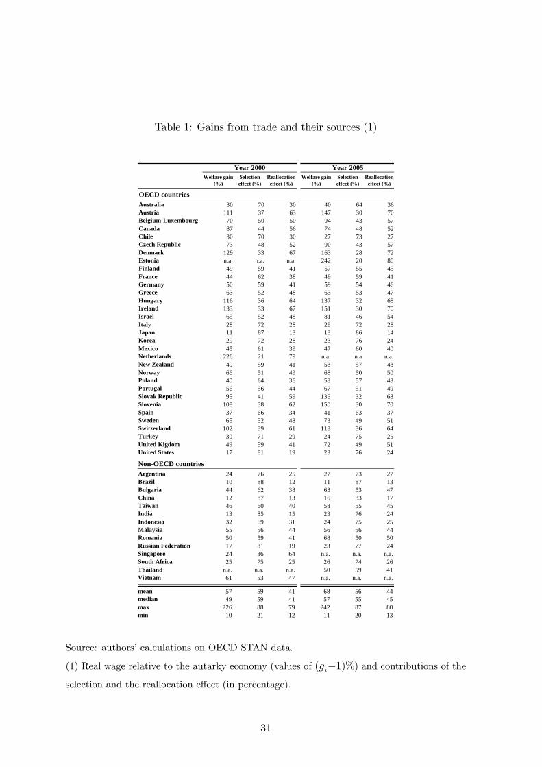
What does the data show about the size of these two e¤ects? Table 1 provides
a quanti�cation of the welfare gains from trade as well as the contribution of the
selection and reallocation e¤ect for a sample of 46 advanced and developing countries
in two di¤erent years, 2000 and 2005. Given that the Ricardian theory laid out in
this chapter best describes trade in manufactures, rather than in natural resources or
primary goods, we follow the literature and consider data on the values of domestic
production, exports and imports � which is all is needed to compute the gains from
trade as well as the contribution of their sources � all referred to the manufacturing
sector.29 In addition, given that the model assumes that trade is balanced, in the
application we impose that exports are identical to imports (equal to their average).
The gains are computed using equation (20), taking the value of the main para-
meters from literature. In particular, we assume that the shape parameter is � = 4,
as advocated by Simonovska and Waugh (2014b), and the share of intermediate goods
in production is � = 0:33, a conventional measure of the share of value added in total
output. The share of the gains from trade pertaining to the selection and reallocation
e¤ects, respectively equal to �i;o and 1� �i;o, are computed using equation (21).
29Data on the value of output (i.e. value added plus intermediate goods) of the manufacturing sector
is often available only at �ve year intervals, especially for small countries (see also Levchenko and
Zhang, 2013). In addition, emerging countries typically have data only for very short time horizons.
Here we solve the trade-o¤ between number of countries and number of years by including in the
sample 46 countries (a larger number than the 19 OECD countries considered by Eaton and Kortum,
2002, albeit smaller than the 60 countries considered by Alvarez and Lucas) and by considering two
di¤erent years (against the practice of considering only one single year). A remarkable exception is
Levchenko and Zhang (2013), who set up a dataset encompassing 72 countries over 5 decades, using
the UNIDO Industrial Statistics Database. Here we prefer to stick to the OECD STAN dataset, which
is generally considered to have higher quality data.
(1) Real wage relative to the autarky economy (values of (gi�1)%) and contributions of theselection and the reallocation e¤ect (in percentage).
31
For each year, Table 1 shows the percentage increase in welfare due to interna-
tional trade and the shares (in percentage) due to the selection and the reallocation
e¤ect. Results show that the gains from trade are considerable (for the cross-country
average welfare is almost 60 and 70 percent higher than in autarky in 2000 and 2005).
As it is well known, the size of the gains is quite sensitive to the assumptions about
the value of the shape parameter and the share of intermediate goods in production.
For instance, by taking � = 6:66 instead of � = 4 (as Alvarez and Lucas, 2007), the
gains would be about 60 percent of those reported in Table 1. By the same token, in
the model without intermediate goods (� = 1), gains from trade would be about one
third of those reported in the table.
Overall, the size of the selection e¤ect is somewhat more important than the real-
location e¤ect in our sample of countries (it is close to 60 percent in the year 2000 and
around 55 per cent in 2005). It is worth noting that, unlike the gains from trade, the two
shares remain unchanged irrespectively of the exact value of � and �. Unsurprisingly,
the reallocation e¤ect is more important in small open economies, such as Denmark,
Estonia, Ireland, the Netherlands, Slovenia, Singapore, Thailand, and Vietnam. For
these countries, the share of the welfare gains pertaining to the reallocation e¤ect is
above 70 percent in at least one year. On the other hand, for large and relatively more
closed countries, it is the selection e¤ect that it is dominant. For instance, among the
OECD economies, only the United States and Japan record a share of the welfare gains
pertaining to the selection e¤ect above 80 percent in at least one year. Among non-
OECD economies, only the BRIC countries (Brazil, Russia, India, and China) show
the same record as the United States and Japan.
5 Conclusion
This chapter provides a deconstruction of the sources of the welfare gains from trade in a
Ricardian model. Under general distributions of industry e¢ ciencies, welfare gains arise
from two distinct sources. The former is an e¤ect due to the selection of industries that
survive international competition. The latter is related to the reallocation of workers
away from the industries that shut down, as well as from those selling only in the
domestic market, to the industries that start servicing the foreign market. If industry
32
e¢ ciencies are Fréchet distributed, so that the model becomes one of the quantitative
trade models of Arkolakis, Costinot and Rodríguez-Clare (2012), these two e¤ects can
be easily measured.
Our results also show that the share of the welfare gains due the reallocation e¤ect
is larger, the larger is the overall welfare gains. Thus, countries that can potentially
gain more from trade � i.e. small open economies that are close to large, rich, and less
e¢ cient markets � would gain mostly from the reallocation e¤ect. Therefore, to fully
reap the bene�ts from international trade, they must be ready to favor the reallocation
of resources towards exporting industries, for example supporting workers�education
and training.
The key insight from our analysis, however, is that quantitative trade models
seem to be useful not only in order to assess the overall welfare gains, but also to
properly measure their sources � an issue that deserves to be further explored in
future studies tackling other models in this class. The route taken in this chapter of
using quantitative trade models to measure not only the overall welfare gains from
trade, but also the contribution of their sources, appears to be a promising area for
theoretical and empirical research.
33
Appendix
A Welfare decomposition with many countries
In order to prove equation (13), let us start by generalizing the resource constraint (9)
to a context with more than just two countries. As in the two-country case, we still
have: qi (j) = 0, if j 2 Oi;z and qi (j) = ci (j) =�, if j 2 Oi;d. Now consider the set ofindustries of country i that export in (and only) the countries n, h, ..., and k, for any
fn; h; :::; kg 2 f1; :::; Ng n fig, and denote this set by On;h;:::;ki;e ;30 the resource constraint
for these industries becomes:
qi (j) =1
�[ci (j) + cn (j) dni + ch (j) dhi + :::+ ck (j) dki] .
Solving the resource constraint for the number of workers in industry j, we obtain:
Li (j) =
8>>><>>>:0 if j 2 Oi;z
z��1i (j) ��wipi
��(1��)Li if j 2 Oi;d
z��1i (j) ��wipi
��(1��)Li � (1 + kni + khi + :::+ kki) if j 2 On;h;:::;ki;e
, (22)
where the terms kli are de�ned as in equation (11), for any destination market l.
Note that the sets Oi;z, Oi;d, On;h;:::;ki;e (for any fn; h; :::; kg as above) form a par-
tition of the set of tradable goods. By aggregating across industries both sides of
equation (22), we obtain the following:�wipi
��(��1)= �i;d�E
�Z��1i;d
�+:::+�i;e;n;h;:::;k�(1 + kni + khi + :::+ kki)�E
�Z��1i;e;n;h;:::;k
�+:::
(23)
where �i;d is the probability that an industry of country i survives international compe-
tition and serves only the domestic market (i.e. �i;d = Pr(Zi 2 Oi;d)); �i;e;n;h;:::;k is theprobability that an industry of country i exports in (and only) countries n, h, ..., and
30The analytical de�nition of On;h;:::;ki;e is as follows: this set includes all the industries that export
in countries n, h, ..., and k, i.e. those for which zi (j) =ci > zl (j) dli=cl, for l = n; h; :::; k; and excludes
those that export in countries di¤erent from n, h, ..., and k, i.e. those for which zi (j) =ci < zl (j) dli=cl
for l 6= n; h; :::; k.
34
k (i.e. �i;e;n;h;:::;k = Pr(Zi 2 On;h;:::;ki;e )); Zi;e;n;h;:::;k is the distribution of the e¢ ciencies
of these industries (i.e. Zi;e;n;h;:::;k = ZijZi 2 On;h;:::;ki;e ). Considering that:
�i;o � E�Z��1i;o
�= �i;d � E
�Z��1i;d
�+ :::+ �i;e;n;h;:::;k � E
�Z��1i;e;n;h;:::;k
�+ ::: ,
we can conveniently rearrange the right-hand side of equation (23) into the sum of
two terms, given by equations (14) and (15). By taking the 1=� (� � 1) power of bothsides, we �nally obtain equation (13).
B Welfare decomposition and average prices
Recall that, in the two-country example, the price of good j in country i is ci=zi (j)
if the good is domestically produced; it is cndin=zn (j) if the good is imported (from
country n). Then, we can write:
pi =
�Zj
[pi (j)]1�� dj
�1=(1��)=
"c1��i
Zj2Oi;o
[zi (j)]1�� dj + (cndin)
1��Zj2Oi;z
[zn (j)]1�� dj
#1=(1��)
= ci �"�i;o � E
�Z��1i;o
�+ (1� �i;o) �
�cndinci
�1��� E�Z��1n;e;i
�#1=(1��).
The �rst term in the square bracket, multiplied by ci, is the average price of domestically-
produced goods, and depends only on the e¢ ciency distribution of the domestic indus-
tries that survive international competition, Zi;o. The second term, multiplied by ci, is
instead the average price of imported goods, and depends on the e¢ ciencies of foreign
exporters, Zn;e;i.
Using the fact that ci = w�i p1��i for any country i, we obtain:
wipi=
"�i;o � E
�Z��1i;o
�+ �i;e
�cndinci
�1��� E�Z��1n;e;i
�#1=�(��1)(24)
Equation (24) shows two main facts. First, it shows that country i�s welfare depends on
the e¢ ciency distribution of domestic industries as well as on the e¢ ciency distribution
of those foreign industries from which country i imports goods, i.e. the e¢ ciencies of
foreign exporters. Second, by comparing it with equation (12), it shows that the
35
selection e¤ect (which coincides with �rst term in the square bracket in (24)) measures
the welfare gains obtained from lower average domestic prices; on the other hand, the
reallocation e¤ect, which is the complement of the selection e¤ect (just like the second
term in the square bracket is the complement of the �rst term in (24)), is equivalent
to the welfare gains due to lower import prices.
For what concerns the reallocation e¤ect, in particular, notice that in Section 3,
by using the resource constraint (which is equivalent to the balanced-trade condition),
we have been able to use the distribution of domestic exporters in the decomposition
(12), instead of the distribution of foreign exporters as in the alternative decomposition
(24). In other words, the resource constraint makes it possible to shift the focus from
imports to exports, i.e. from the e¢ ciencies of foreign exporters to the e¢ ciencies of
domestic exporters.
36
CHAPTER 2
Trade-Revealed TFP
37
38
1 Introduction
Estimating the level of a country�s total factor productivity (TFP) is a very di¢ cult
task. The standard development-accounting (or "level-accounting") approach consists
in choosing a functional form for the aggregate production function, measuring the
quantities of output and inputs, and then obtaining TFP as a residual (King and
Levine, 1994). In general, the derivation of quantity data is a very critical part of this
approach. Recent literature, such as Burstein and Cravino (2015), has in fact shown
that the common practice of obtaining quantity data by de�ating value data may be
�awed, because the price indexes calculated by statistical agencies that are adopted for
this purpose di¤er from the ideal de�ators that would be appropriate from a theoretical
standpoint.1
Another important problem of the standard methodology is related to the fact
that TFP is measured as a residual. As such, TFP incorporates any statistical error
in the data and ends up being a "measure of our ignorance" (Abramovitz, 1956).
The need to re�ne existing methodologies and complement them with new ones
is warranted by the importance of TFP for understanding the distribution and growth
of wealth across nations. In particular, studies based on development accounting show
that di¤erences in TFP account for a big chunk of cross-country di¤erentials in per
capita income (e.g. Hall and Jones, 1999). In addition, while recent research has
conjectured that these results might be due to sectoral di¤erences in TFP levels, this
hypothesis can be tested only on very rough sectoral classi�cations.2
1Similarly, the measurement of the quantity of physical capital is especially troubling, because even
the basic value data have to be constructed. In addition, the perpetual inventory method commonly
adopted for this purpose is very demanding in terms of data (for instance, it requires long time series
on �xed investments and price de�ators), entails heroic assumptions about the depreciation rate,
mixes up types of capital with di¤erent e¢ ciencies, and neglects key issues regarding the quality of
capital. Di¢ culties then escalate if one is interested in calculating homogeneous measures of TFP
across several countries or sectors. In fact, cross-country heterogeneities in the quality of capital and
in the di¤usion and accuracy of price de�ators are especially large across industrial and developing
countries. The lack of sectoral data on �xed investment, which a¤ects even some industrial economies,
is also stunning.
2For di¤erent views about this hypothesis see Caselli (2005), who considers data disaggregated into
two sectors (agriculture and non-agriculture), and Herrendorf and Valentinyi (2012), who extend the
39
In this chapter, we use a structural model of international trade to measure TFP.
The logic of our approach is to derive TFP not from its "primitive" (the aggregate
production function), but from its observed implications. The model, in fact, maps
international trade �ows, production, and wages into the average productivity of the
tradeable goods sector, allowing to obtain a proxy for the TFP of this sector.
The new road that we explore builds on the Ricardian model developed by Eaton
and Kortum (2002) and some theoretical results obtained in a companion paper by
Finicelli, Pagano, and Sbracia (2013), which we extend in this chapter. In the Eaton-
Kortummodel, industry productivities in the tradeable goods sector of each country are
described by a Fréchet distribution, whose country-speci�c scale parameter is related
to the average productivity of the closed economy. Eaton and Kortum (2002) have
shown that this parameter can be estimated, relative to that of a benchmark country,
using value data on bilateral trade �ows, production and nominal wages. For the
open economy, Finicelli, Pagano, and Sbracia (2013) have proven that the productivity
distribution of the industries that survive international competition remains a Fréchet
and that the mean of this distribution is equal to the average productivity under
autarky, augmented by an easy-to-quantify measure of trade openness. Here, we �rst
show formally that the average productivity across domestic industry provides a proxy
for the TFP and, then, we take the former as our measure of productivity, which
we dub trade-revealed TFP. The approximation error is nil in the extreme cases of
autarky and zero gravity; in the intermediate case of positive but �nite trade barriers,
the approximation error, however, is low not only when the set of exporters is small
(as the bias a¤ects few exporting industries), but also when it is large. In the latter
case, in fact, because foreign demand does not alter the composition of the demand
for domestic goods (foreign and domestic consumers have the same preferences), then
almost all industries are equally a¤ected by the same bias. In other words, in this case
the problem becomes the larger weight than in TFP that the simple average gives to
the industries that do not export, which are few when trade barriers are small.
We then turn these theoretical results into estimates of the TFP of the tradeable
goods sector of 19 OECD countries, relative to the United States, with annual data
analysis to �ve sectors.
40
from 1985 to 2002.3
With respect to the development-accounting approach, our estimates have three
main advantages. First, they are no longer mere residuals, but are the productivities
that best �t data on trade, production and wages. The reason is that the country-
speci�c scale parameter related to average productivity a¤ects, together with wages,
all the bilateral exports of this country as well as the domestic production sold domes-
tically. Therefore, in a model with N countries, each scale parameter can be estimated
using N � 1 observations (i.e. N(N � 1) observations to estimate N parameters). The
estimation process that is involved, in turn, potentially allows to reduce the impact of
the statistical error that a¤ects, instead, the standard methodology.
Second, our estimates are obtained from value data about trade, production and
wages and do not require hard-to-get quantity data. This feature eliminates the critical
step related to the de�ation of quantity data, and ensures a higher degree of homo-
geneity and comparability of data across several countries.
Third, the wide availability of sectoral data on trade �ows, production and wages
makes it possible to compute sectoral estimates of TFP. While in this chapter we only
consider the aggregate tradeable goods sector and do not pursue any �ner classi�cation,
Levchenko and Zhang (2011), based on our methodology, estimate average productiv-
ities for several countries over a 50-year period. Similarly, Shikher (2004) performs
sectoral estimates of the parameter related to average productivity, from which one
could easily retrieve sectoral TFPs following our methodology.
These advantages do not come at no cost. Our estimates refer to the restricted
universe of the tradeable goods sector, which we identify as the manufacturing sector,
rather than embracing the whole economy. They measure TFP in each country as the
average productivity across domestic industries and, therefore, are an approximation of
the TFP that would obtain by aggregating production across industries.4 They provide
3We use the same data sources and sample of countries as Eaton and Kortum (2002). In addition,
while they focus only on one year (1990), we consider a time horizon spanning 18 years. Unfortunately,
one data source was discontinued in 2004, preventing us to analyze a longer time span.
4Finicelli, Pagano, and Sbracia (2013) show that average productivity of domestic industries ap-
proximates the TFP of the economy�s aggregate production function. In the extreme cases of autarky
and zero gravity, the approximation error is nil. In fact, the aggregate production function derived
41
relative levels of TFP across countries, but not their absolute values. Finally, while
our measure is obtained from a model which neglects physical capital, the last is not
necessary because in the model it is the cost of inputs that matters for bilateral trade
shares, not their quantities. When we introduce capital, however, results are broadly
unchanged.
A noteworthy result from our analysis is that the TFP rankings and relative
values that we obtain appear more plausible than those delivered by the standard
development-accounting approach. One key di¤erence with respect to development-
accounting studies, most notably Hall and Jones (1999), is that while in their samples
Italy is usually found to have the highest TFP, a surprising result given the relative
weakness of institutions and government policies ("social infrastructure") in this coun-
try, according to our analysis Italy ranks only 6th or 7th over the whole sample period,
and the most productive country is invariably the United States.5 Interestingly, in our
sample of countries the correlation between TFP and Hall and Jones�social infrastruc-
ture index is higher if TFP is measured using our methodology than with their own
TFP data.
We then provide a zoom shot of the manufacturing TFP of Italy relative to
the United States, comparing the dynamics of our measure with one obtained from
development accounting. We view this case study as especially intriguing because of
the just mentioned "anomaly" of development-accounting results. The focus on this
country pair also allows us to o¤er a more detailed and data-enhanced analysis. We
�nd that our measure yields a sharp di¤erence in levels with respect to development
by aggregating across industries in equilibrium features a TFP that is proportional to the average
productivity, and the proportionality constant, which is the same across countries, cancels out when
one computes relative TFPs. In the intermediate case of positive but �nite trade barriers, average
productivity is a¤ected by a bias: exporters have a smaller weight than in TFP, because their sales to
foreign consumers are not taken into account in the simple average. The approximation error, however,
is low not only when the set of exporters is small (as the bias a¤ects few exporting industries), but
also when it is large. In the latter case, in fact, because foreign demand does not alter the composition
of the demand for domestic goods (foreign and domestic consumers have the same preferences), then
almost all industries are equally a¤ected by the same bias. In other words, in this case the problem
becomes the larger weight than in TFP that the simple average gives to the industries that do not
export, which are few when trade barriers are small.
5For a brief discussion of this point, see Hall and Jones (1999) and Lagos (2006).
42
accounting, while preserving a very similar time pattern.
The focus on input costs (instead of quantities) to measure TFP makes our
methodology reminiscent of the dual method for computing TFP growth rates de-
veloped by Hsieh (2002). However, we do not obtain our TFP as a residual, and we
compute TFP (relative) levels instead of growth rates. Another closely related method
for comparing TFP across countries is the "revealed-superiority" approach of Bar-Shira,
Finkelshtain, and Simhon (2003), which in turn is inspired by Samuelson�s principle
of revealed preferences. With this paper, our methodology shares the idea of mea-
suring TFP not from its "primitive" (the production function) but from its observed
implications. Our approach distinguishes from Bar-Shira, Finkelshtain, and Simhon�s
in that they extract information about the TFP for the whole economy from observed
aggregate pro�ts, while we focus on the TFP of the tradeable goods sector and derive
it from countries�shares in international trade. In addition, we quantify relative TFPs,
while their methodology only delivers a ranking.
Traces of the idea of exploiting the e¤ects of TFP on trade �ows to retrieve a
measure of the TFP itself appear, in di¤erent forms, also in other papers. Tre�er (1995)
obtains Hicks-neutral factor-augmenting productivities for several countries (relative to
the United States) as the productivities that minimize the gap between observed trade
data and the trade pattern implied by factor intensities according to the Hecksher-
Ohlin-Vaneck theory. Waugh (2010) obtains a relationship between model parameters
and TFP using a variant of the Eaton-Kortum model with traded intermediate goods
and a non-traded �nal good; then, he quanti�es the contribution of international trade
to the TFP without estimating the latter. Fadinger and Fleiss (2011) develop a model
with monopolistic competition and homogeneous �rms � whereby we assume perfect
competition and heterogeneous industries � but end up with an empirical framework
to measure TFP that turns out to be similar to ours, in that it requires only data on
trade �ows, production and input costs.
Here is a roadmap of the chapter. Section 2 brie�y summarizes the Eaton-Kortum
model and the main results that provide the theoretical background for the empirical
methodology, which is presented in Section 3. Section 4 computes and describes the
trade-revealed TFPs, compares them with results from a sample of previous studies,
and checks their robustness to the inclusion of physical capital. Section 5 analyzes
43
more closely the case of Italy versus the United States. Section 6 concludes, with some
suggestions for future research.
2 Theoretical underpinnings
The Eaton-Kortum model considers a framework with many countries and a continuum
of tradeable goods produced by industries operating under perfect competition. Making
the quantity qi (j) of the tradeable good j in country i requires the bundle of inputs
Ii (j), in a constant-returns-to-scale technology; namely: qi (j) = zi (j) Ii (j), where
zi (j) is an e¢ ciency parameter which varies across countries and industries.
The key hypothesis in Eaton-Kortum is that each zi (j) is the realization of a
country-speci�c random variable Zi, with Zi � Fr�echet (Ti; �), where Ti > 0, � > 1,
and the Zi are mutually independent across countries. The two parameters of the
distribution are the theoretical counterparts of the Ricardian concepts of absolute and
comparative advantage. The former � Ti, the state of technology � captures country
i�s absolute advantage: an increase in Ti, relative to Tn, implies a higher share of goods
that country i produces more e¢ ciently than country n. The latter � �, the precision
of the distribution � which is assumed identical across countries, is inversely related to
the dispersion of Zi and its connection with the concept of comparative advantage stems
from the fact that Ricardian gains from trade depend on cross-country heterogeneities
in technologies.6 In this perspective, Eaton and Kortum (2002) demonstrate that a
decrease in � (higher heterogeneity) generates larger gains from trade for all countries.
Another important assumption concerns trade barriers, which are modeled as
iceberg costs: delivering one unit of any good from country i to country n requires
producing dni units (with dni > 1 for i 6= n and dii = 1). Trade barriers lift the priceat which countries can sell their products in foreign markets above the one at which
they sell the same goods at home.
If representative consumers in all countries have identical CES preferences across
tradeable goods, it is possible to show two fundamental properties of the model. First,
6Denoting Euler�s gamma function by �, the moment of order k of Zi is given by Tk=�i �� [(� � k) =�]
if � > k. The connection between � and the dispersion of Zi can be appreciated by considering that
the standard deviation of logZi is �=(�p6).
44
the market share of country i in country n � i.e. the ratio between the value of the
imports of country n from country i (Xni) and the value of the total expenditure (or
total absorption) of country n (Xn) � is given by
Xni
Xn
=Ti � (cidni)��
�n, where: �n =
NXk=1
Tk � (ckdnk)�� , (1)
with ci denoting the cost of the bundle of inputs. This share is increasing in the state
of technology Ti and decreasing in the input cost ci and the trade barrier dni. Its value
depends also on the technologies, costs and trade barriers of any other country k: it
increases with costs ck and distances dnk, and decreases if technologies Tk increase.
Second, the exact price index of the bundle of tradeable goods in country n
resulting from the CES aggregator and the prices pn (j) is
pn = � ��1=�n , where: =��
�� + 1� �
�
��1=(1��), (2)
with � denoting Euler�s Gamma function and � > � � 1.
The solution of the model is given by a system of non-linear equations in relative
wages, relative prices and trade �ows.7 The main testable implication can be obtained
by assuming that intermediate inputs comprise the full set of tradeable goods, so that
the input cost is ci = w�i p1��i , where wi is the nominal wage in country i and pi is given
by equation (2). Rearranging equations (1) and (2) we obtain :
log
"�Xni
Xnn
��Xii=XiXnn=Xn
� 1���
#= Si � Sn � � log (dni) , (3)
where
Si �1
�log (Ti)� � log (wi) , (4)
and Xni is the value of imports of country n from country i, Xn the value of the
total expenditure (or total absorption) of country n, Xnn the value of expenditure on
domestically produced goods, wi the nominal wage in country i. The variable Si, given
by the state of technology adjusted for labor costs, is a measure of the competitiveness
of country i. The left-hand side of equation (3) is a "normalized" share of the imports
7There is also a non-tradeable goods sector in the economy, and a constant fraction of the aggregate
�nal expenditure (equal to 1 � �, 0 < � < 1) is spent on these goods. For the whole solution of themodel, see Eaton and Kortum (2002, pp. 1756-1758).
45
of country n from country i. This equation shows that the ability of country i to sell
its own products in country n is increasing in the relative competitiveness of country
i vis-à-vis n and decreasing in the iceberg cost of exporting from i to n.8
Equation (3) can be used, as in Eaton and Kortum (2002), to obtain estimates of
the relative states of technology in a cross section of countries (i.e. the ratios Ti=Tn).
However, we are interested in estimating TFPs, which are related but far from identical
to the states of technology. In fact, while the mean of Zi is the average productivity
in country i across all existing tradeable goods, with open markets there exist some
industries in country i that cease to produce because they eventually succumb to foreign
competition. The latter happens, precisely, to the industries that make their goods less
e¢ ciently than their foreign competitors, so that these goods are cheaper to import
than to produce at home, despite the advantage provided by trade barriers. Therefore,
E (Zi) corresponds to the TFP of country i only under autarky, while if markets are
open then the TFP must be calculated over the subset of tradeable goods that are
actually made by country i.
This issue is addressed from a theoretical standpoint in Finicelli, Pagano, and
Sbracia (2013), who derive, within the Eaton-Kortum model, the productivity distri-
bution of the industries that survive international competition, also a Fréchet. The
mean of this distribution calculated for country i, that is the TFP of the tradeable
goods sector of this country, denoted with TFPi, can be expressed as follows:
TFPi = E (Zi) � 1=�i = T1=�i � �
�� � 1�
�� 1=�i , (5)
where
i � 1 +IMP i
PROi � EXP i. (6)
The factor 1=�i is a measure of trade openness that captures the e¤ect of international
competition in selecting industries that have a competitive advantage.9 Equation (5)
8The fact that quantity-data on physical capital are not needed in our methodology is by no means
driven by the omission of this factor from the production function. As equations (3) and (4) show, in
fact, although labor is included in the production function, its cost, and not its quantity, is relevant
for bilateral trade shares. By the same token, if physical capital is added to the production function,
equations (3) and (4) become functions of both wages and the cost of capital, but do not depend on
the capital stock (see Section 4 and Appendix C for details).
9Notice that the selection e¤ect is always positive (TFPi > E (Zi)). In other words, industries
46
forms the basis of our estimates of cross-country relative TFPs: once the relative states
of technology are estimated, measuring relative TFPs requires only widely available
data on trade and production.
3 Empirical methodology
In this section, we illustrate the methodology to estimate the TFP of the manufacturing
sector and apply it to a sample of 19 OECD countries for each year between 1985 and
2002. The methodology follows three main steps. First, equation (3) is used to estimate
the competitiveness indexes Si. Second, the states of technology Ti are derived from the
estimated Si, using equation (4). In applying these two steps, we provide an extension
of the cross-section analysis performed by Eaton and Kortum (2002) with 1990 data,
to a sample period spanning 18 years. In addition, we update the original methodology
of Eaton and Kortum (2002) in that we convert nominal wages into U.S. dollars using
PPP instead of market exchange rates, as suggested by Finicelli, Pagano, and Sbracia
(2011). Once states of technology are obtained, it is immediate to compute our trade-
revealed TFPs from equations (5) and (6), a step that we �nalize in Section 4. We
defer to Appendix A a detailed description of our dataset.
Let us consider equation (3). The left-hand side can be measured with production
and trade data, and a calibration for �. For �, we follow Alvarez and Lucas (2007)
who de�ne it as the cross-country average of manufacturing value added over gross
manufacturing production. By doing so, they consider labor and capital goods as
part of a single production factor, which they label as "equipped labor". Over the
period 1985-2002 this calibration delivers annual values of � between 0:31 and 0:34.10
that survive international competition are on average more productive than those that are crowded
out, implying that the TFP of the open economy is above the autarky level. Finicelli, Pagano, and
Sbracia (2013) focus on this result and show that it holds under very general assumptions about the
distribution of productivities. In particular, it holds irrespectively of the correlation among country
technologies, for several classes of joint distributions, including the multivariate Fréchet, Pareto, nor-
mal, and lognormal. With independent technologies, the result always holds, irrespectively of the type
of their joint distribution.
10Eaton and Kortum (2002) use an alternative calibration, setting � equal to the cross-country
average of the labor share in gross manufacturing production. This calibration implies that labor is
47
On the right-hand side, trade barriers can be modeled using the proxies suggested by
the gravity literature. Following Eaton and Kortum (2002), we proxy trade barriers
between i and n with a set of standard dummy variables, namely:
log dni = dk + b+ l + e+mn , (7)
where the dummy variables associated with each e¤ect are suppressed for notational
simplicity. In equation (7), dk is the e¤ect of the distance between i and n lying in
the k-th interval (k = 1; :::; 6);11 b is the e¤ect of i and n sharing a border; l is the
e¤ect of i and n sharing the language; e is the e¤ect of both i and n belonging to the
European Economic Community (EEC), from 1985 to 1992, or to the European Union
(EU), from 1993 onwards; mn (n = 1; :::; 19) is a destination e¤ect.
Using (7), equation (3) becomes
log
"�Xni
Xnn
��Xii=XiXnn=Xn
� 1���
#= Si � S 0n � �dk � �b� �l � �e , (8)
where S 0n = Sn + �mn. The competitiveness of country i is estimated as the source
country e¤ect (Si), while the destination dummies (S 0n) are the sum of country n0s
competitiveness (Sn) and destination e¤ect (�mn). To avoid perfect multicollinearity,
we impose the same restriction as Eaton and Kortum (2002) thatP
n Sn =P
n S0n = 0;
therefore, the estimated coe¢ cients of these dummy variables measure the di¤erential
competitiveness e¤ect with respect to the average (equally-weighted) country.
We estimate equation (8) by ordinary least squares for each year (separately) in
the period 1985-2002.12 With 19 countries, we have 342 informative observations for
each regression (the equation is vacuous when n = i). Table 1 reports the results of
the regressions for the �rst and last year of our sample, and for 1990 (the benchmark
year in Eaton and Kortum, 2002). The coe¢ cients of the distance dummies indicate,
as expected, that geographic distance inhibits trade. However, the size of this e¤ect
the sole production factor and that capital goods are comprised into intermediate goods. Over our
sample period this approach returns annual values of � between 0:19 and 0:22. Section 4 provides a
battery of robustness tests, in which we analyze the sensitivity of our results to this as well as other
calibrations.
11Intervals are speci�ed in Table 1, with distance calculated in miles.
12By running a regression for each year, we end up with yearly estimates of the main parameters
and, then, of average productivities.
48
tends to decline over time, perhaps suggesting an increasing degree of integration not
captured by other e¤ects. In addition, the decline appears to be sharper for the biggest
distances. The dumping e¤ect of distance is mitigated by positive border and language
e¤ects. Belonging to the EEC/EU also tends to foster trade, although this e¤ect is not
statistically signi�cant, which comes as no surprise given that most countries in the
sample are European.
Estimates of the source dummies Si indicate that in 1985 Japan is the most
competitive country, followed by the United States, while the ranking between these
two countries inverts towards the end of the sample period. On the other hand, Greece
and Belgium stand out as the least competitive countries throughout the whole period.
Relative to the United States, competitiveness of most countries in the sample peaks
towards the end of the 1980s, then declines until 2000, and recovers somewhat in 2001-
02.
Estimates of ��mn provide a measure of how cheap it is to export manufacturing
goods to country n, compared to the average.13 The values of��mn re�ect the presence
of tari¤s and non-tari¤ costs that have to be paid by foreigners to sell a good in the
domestic market, such as local distribution costs, legal obligations, product standards.
Over the entire sample period, the country ranking of ��mn is similar to that Sn;
for instance, Japan is the cheapest destination, while Belgium stands out as the most
expensive one.14
From Si, we can now extract the states of technology Ti simply by inverting
equation (4), i.e. Ti = exp (�Si) � w��i . This step requires data on nominal wages and
13Waugh (2010) estimates equation (8) by including a source- instead of a destination-country
dummy. In his sample, which includes both advanced and developing economies, this method returns
a positive correlation between the Si and income per worker, consistently with some stylized facts
documented in that paper. In our sample, which comprises only developed economies, Waugh�s
method would return a negative correlation of the Si with income per worker (in the order of -0.2)
against a positive correlation (0.3) from our method.
14Eaton and Kortum (2002) estimate equation (8) by generalized least squares, using only 1990
data, obtaining similar results in terms of sign and signi�cance of the coe¢ cients and of country
ranking. (See, in particular, their discussion concerning the apparently surprising result about the
high degree of openness of Japan.) The small di¤erences between our results and theirs are due only
to the di¤erent calibration of � and to the older update of the OECD data used in their paper, and
not to the di¤erent estimation method.
49
Table 1: Bilateral trade equation in selected years (1)
(1) Estimates of equation (8) using OLS; standard errors in brackets.
50
a calibration for �.
Following Eaton and Kortum (2002), nominal wages are adjusted for education to
account for the di¤erent degrees of "worker quality" among the countries in our sample.
We set wi = compi �exp (�g � hi), where compi is the nominal compensation per worker,g the return on education (which we set to 0:06 as Eaton and Kortum, 2002), hi the
average years of schooling.15 Wages are converted into a common currency using PPP
exchange rates, as suggested by Finicelli, Pagano, and Sbracia (2011).16 This approach
is also consistent with the standard practice in development accounting, which is the
yardstick for our trade-revealed TFPs.
The parameter � is set equal to 6:67 as in Alvarez and Lucas (2007), who exploit
the fact that the expression for market shares derived in Eaton and Kortum (2002)
is identical to one obtained in a model à la Armington (1969), with � replacing Arm-
ington�s �a � 1, where �a is the Armington elasticity. Based on Anderson and vanWincoop (2004), Alvarez and Lucas pick their preferred calibration from a range of
values between 4 and 10.17
Table 2 shows the values of the resulting states of technology, at the 1=� power, rel-
ative to those of the United States in selected years. We report the values of (Ti=Tus)1=�,
where the subscript us stands for the United States, because this ratio is equal to
E (Zi) =E (Zus) (see footnote 7 for the mean of the Fréchet), that is, as discussed in
15Setting g = 0:06 is a conservative calibration according to Bils and Klenow (2000). See Appendix
B for results with the somewhat larger (and non-linear) values of the return on education used by
Hall and Jones (1999) and Caselli (2005).
16Finicelli, Pagano, and Sbracia (2011) document that, by converting wages into a common currency
using market exchange rates, as originally suggested by Eaton and Kortum (2002), the resulting
estimates of relative technologies show implausible swings for several countries. Most importantly,
the time-series of these estimates exhibit a correlation with nominal exchange rates vis-à-vis the US
dollar that, for many countries, is not signi�cantly di¤erent from �1 (a negative correlation meansthat a depreciation of a country�s currency vis-à-vis the US dollar is associated with a decrease in its
relative state of technology).
17Following a di¤erent approach, Eaton and Kortum (2002) estimate � using other testable impli-
cations of the model and �nd values between 3 and 13 (their benchmark is 8:28). Notice that both
Alvarez and Lucas (2007) and Eaton and Kortum (2002) consider cross-sectional data. In our empiri-
cal analysis spanning 18 years, we take � time-invariant. Finicelli, Pagano, and Sbracia (2011) provide
some evidence supporting this assumption.
51
Table 2: States of technology in selected years (1)
The �nding that the United States�TFP is the highest throughout the two-decade
period is worth stressing. According to a number of studies based on development
accounting, in fact, in the mid-1980s to early-1990s it was Italy�s TFP that ranked
�rst among the 19 countries in our sample.19 These �ndings appear rather odd given
the well known relative weakness of Italy�s institutions. For example, Lagos (2006) is
puzzled by the result that TFP is higher in Italy than in the United States, which is at
odd with the observation that Italy has a more distorted labour market vis-à-vis the
United States. Similarly, Hall and Jones (1999) underscore that hours per worker "are
higher in the United States than in France and Italy, making their [high] productivity
levels more surprising." Our methodology returns a more plausible assessment, whereby
in our sample of high-income countries Italy ranks 6th or 7th, with a manufacturing
TFP that is 13% to 17% lower than that of the United States.
Besides the speci�c result for Italy, which is analyzed with greater detail in the
next section, our �ndings are broadly in line with those from a sample of other studies
that use di¤erent methodologies. The rank correlation of our 1990 results with the
19See, for example, Hall and Jones (1999), Chari, Restuccia, and Urrutia (2005), or the development-
accounting excercise performed by Fadinger and Fleiss (2011). In Klenow and Rodríguez-Clare (1997),
the TFP of Italy is third, but it is still higher than that of the United States.
55
TFP ranking estimated by Bar-Shira, Finkelshtain, and Simhon (2003) is above 0:8.
The (linear) correlation of our 1985 results with the 1983 "trade-revealed type" of
TFP provided by Tre�er (1995) is about 0:7.20 The broad picture delivered by our
methodology is also not too di¤erent from that in Klenow and Rodriguez-Claire (1997)
and Hall and Jones (1999): the correlation between their relative TFPs and ours are
fairly high, equal to about 0:65 in both cases.21
Figure 2: TFP and social infrastructure (1)
AS
AUBE
CA
DKFI
FR
GE
GR
IT
JP
NT
NO
PO
ES
SW
UK
NZ
US
y = 1.06x 1.03R2 = 0.19
0.5
0.4
0.3
0.2
0.1
0.0
0.1
0.2
0.3
0.55 0.65 0.75 0.85 0.95Social infrastructure (Hall and Jones, 1999)
log
TFP
(Hal
l and
Jon
es, 1
999)
AS
AU
BE
CA
DKFI
FRGE
GR
IT JP NT
NO
PO
ES SW
UK
NZ
US
y = 0.83x 0.93R2 = 0.34
0.5
0.4
0.3
0.2
0.1
0.0
0.1
0.2
0.3
0.55 0.65 0.75 0.85 0.95Social infrastructure (Hall and Jones, 1999)
log
TFP
(Tra
der
evea
led)
(1) Data refer to 1988 in both pictures. TFP is relative to the United States.
It is worth recalling the result documented by Hall and Jones (1999) who �nd
that, in a sample of 127 countries, di¤erences in social infrastructure drive di¤erences
in capital accumulation, productivity, and output per worker. The positive correlation
between their measure of TFP and their index for social infrastructure remains also
if one narrows the analysis to the 19 advanced economies of our sample (left panel of
Figure 2). Yet, in that scatter plot some countries � notably Italy, but also France
and Spain � display very large residuals from a simple OLS regression, featuring a
much higher TFP than the predicted one. Interestingly, using our trade-revealed TFPs
(right panel of Figure 2) delivers a stronger correlation and a better �t of the data (R2
20Tre�er (1995) obtains the Hicks-neutral factor-augmenting productivities of several countries (rel-
ative to the United States) that provide the smallest gap between observed trade data and the trade
pattern implied by factor intensities. While the purpose of his study was not that of measuring TFP
(but, rather, that of vindicating the predictions of the Hecksher-Ohlin-Vaneck theory), his results
provide the �rst example of a trade-revealed measure of TFP.
21The estimates in Kleenow and Rodriguez-Claire refer to year 1985, those in Hall and Jones to
1988. The correlations are obviously calculated with respect to our estimates for the corresponding
years.
56
climbs from 19 to 34 percent), while solving the TFP "anomalies" of Italy, France, and
Spain, that present a much smaller residual in the new regression.
Are our measures robust to the inclusion of physical capital in the model? In
this case, estimating the relative states of technology requires data on the rental cost
of capital. Assume that the production function for good j in country i is given by
qi (j) = zi (j)�L�i (j)K
1��i (j)
��I1��i (j) . (10)
Denoting with TKi the state of technology in country i when capital is included in the
production function, in Appendix C we show that
TKiTKj
=TiTj��ri=wirj=wj
�(1��)��(11)
where ri denotes the rental cost of capital, and Ti is still the state of technology in
the benchmark model without capital. Note, �rst, that if ri=wi = rj=wj 8i; j, thenthe models with and without capital bear identical results for the states of technology
and the TFPs. For the case in which this restrictive assumption is not ful�lled, we
verify the robustness of our �ndings to the inclusion of capital by computing the cor-
responding TFPs relative to the United States that, in analogy with (9), are given by
�Ki =�TKiTKus
ius
� 1�. Maintaining � = 0:33 and � = 6:67, and calibrating the additional
parameter � = 0:33, we compute the �Ki using data for 1996 and di¤erent sources for
ri.
In particular, we provide four di¤erent estimates (the results are shown in Figure
3, which plots �Ki against �i). As a �rst special case, we assume that ri = r 8i, so thatin (11) the cost of capital cancels out and the corresponding data are not necessary
(north-west panel in the �gure). Second, after removing the hypothesis of cross-country
equality of the cost of capital, we compute �Ki using the estimates of ri from Caselli and
Feyrer (2007; north-east panel). Third, using the �rst-order condition from the cost
minimization problem that ri=wi = (1� �) =�ki, where ki is the capital-labor ratio,we express (11) as a function of ki, instead of ri=wi, and compute the �
Ki using the
estimates of ki from Caselli and Feyrer (2007; south-east panel). Finally, we change
the estimates of both ri and wi and take them from Waugh (2010; south-west panel).22
22Waugh (2010) computes equilibrium wages from trade shares by imposing balanced trade (equa-
tion 3, page 7. in his paper), instead of using actual data. Wages, in turn, in combination with
57
Figure 3 shows that the results obtained with capital in the production function
compare rather well with our benchmark estimates, with a high correlation between
�Ki and �i in all four cases. We can thus conclude that our results are robust to the
fact that the model by which they are drawn does not provide an explicit role for the
stock of physical capital.23
Figure 3: A comparison of TFPs with and without capital (1)
AU
AT
BE
CA
DE FI
FR
GR
IT
JP
NE
NZNO
PO
ESSW
UK
US
GE
0.6
0.7
0.8
0.9
1.0
0.6 0.7 0.8 0.9 1.0Benchmark relative TFPs (model without capital)
Rel
ativ
e TF
Ps w
ithr
equa
l acr
oss
coun
trie
s
Correlation = 0.84
AU
AT
BE
CA
DEFI
FR
GR
IT
JP
NE
NZ
NO
PO ES
SWUK
US
0.6
0.7
0.8
0.9
1.0
0.6 0.7 0.8 0.9 1.0
Benchmark relative TFPs (model without capital)
Correlation = 0.70
Rel
ativ
e TF
Ps w
ithr
from
Cas
elli
and
Feyr
er (2
007)
AU
AT
BE
CA
DEFI
FR
GRIT
JP
NE
NZ
NO
PO
ESSW
UKUS
0.6
0.7
0.8
0.9
1.0
0.6 0.7 0.8 0.9 1.0Benchmark relative TFPs (model without capital)
(1) Data refer to 1996 in all pictures. TFP is relative to the United States.
aggregate capital-labor ratios, are used to determine the rental costs of capital. We thank Mike
Waugh for sharing his data with us.
23We also estimate the relative TFPs using, alternatively, data on the capital-labor ratios in Kleenow
and Rodriguez-Claire (1997) and in Hall and Jones (1999). Consistently with these papers, we use data,
respectively, for 1985 and 1988. In both cases, the results with and without capital are comparable,
with correlations between �Ki against �i equal to 0.65.
58
5 A case study: Italy vs. the United States
The methodology that we propose to estimate TFPs marks a neat departure from
the standard approach. It is therefore interesting to enhance the comparison of our
results with those from development accounting. We perform this exercise for the whole
1985-2002 period for Italy versus the United States, which is a particularly interesting
case given the aforementioned "Italian anomaly" from development-accounting studies.
This case also allows us to re�ne the measurement of labor inputs by adjusting wages
for working hours, which are available for both countries at the sectoral level.24 The
limited availability of the necessary data to implement the development-accounting
methodology prevents us from extending the comparison to all the countries in the
sample.25
We start from the standard assumption in development accounting that output
in country i (Yi) is given by: Yi = AiK�i H
1��i , where Ai is the TFP, Ki the stock of
physical capital with share �, and Hi the stock of human-capital augmented labor.
Assuming that each worker in country i has been trained with hi years of school-
ing, human-capital augmented labor is given by Hi = Li � exp (g � hi), where Li is thetotal number of worked hours and g = 0:06 as in the previous section.
24Recall that Hall and Jones (1999) were especially concerned by the high TFP of Italy because of
the lower number of hours worked in this country vis-à-vis the US. Therefore, accounting for working
hours also allows us to explicitly address their concern.
25The measurement of physical capital is the step in which data limitations are stronger. For
instance, from OECD STAN, the main source of comparable cross-country data on production at the
sectoral level, the volume of net capital stock � a common proxy for physical capital � is available
for the whole sample period for the manufacturing sector of only four countries (Denmark, France,
Italy, and Spain). The volume of gross capital stock � a measure in which capital depreciation is
neglected and di¤erent capital assets are not weighted � is available only for six additional countries
(which do not include major countries such as the United States and Japan). Similar problems arise if
one tries to calculate the stock of capital from manufacturing investments. OECD STAN provides the
volume of �xed investment in the manufacturing sector of 11 countries during our sample period (and,
again, not for large countries such as Japan and the United Kingdom). The value of manufacturing
investment is available for almost all countries (15 out of 19) but, then, one faces the critical issue of
�nding an appropriate price de�ator. Schreyer and Webb (2006) provide a useful survey of de�nitions
and data availability of capital stock measures.
59
Figure 4: Manufacturing TFP of Italy relative to the US (including worked hours)
Gravity data. Geographic distances and border dummies are from Jon Haveman�s
International Trade Data (http://www.macalester.edu/research/economics/page/Haveman/
Trade.Resources/TradeData.html). Countries are grouped by language as in Eaton
and Kortum (2002): (i) English: Australia, Canada, New Zealand, United Kingdom,
United States; (ii) French: Belgium and France; (iii) German: Austria and Germany.
Wages and schooling data. Annual compensation per worker in the manufacturing
sector is from OECD-STAN. Values are converted into a common currency using the
PPP exchange rates available from the OECD. Wages are then adjusted for education,
as explained in Section 3. Years of schooling are obtained from de la Fuente and
Doménech (2006). We deal with missing data by interpolation and extrapolation using
the most recent update of the dataset �rst presented in Barro and Lee (2000).
Development-accounting methodology and data. Capital stock data are obtained
from real investment using the perpetual inventory method, according to the following
relationship:
Kt = It + (1� �)Kt�1
where It is real investment and � the depreciation rate, which we set equal to 0:06 as
in Caselli (2005). Real investment in PPP in the manufacturing sector is computed
as RGDPL�POP�KI�IM, where RGDPL is real income per capita in PPP, POP is
population, KI is the total investment share in total income, and IM is the investment
share of the manufacturing sector in total investment. The variables RGDPL, POP,
and KI are from the Penn World Tables 6.2; IM is computed from OECD STAN.
63
Following the standard practice, initial capital stock is computed as K0 = I0= (� + �) ;
where I0 is the oldest available value in the investment series (which start in 1970 for
both Italy and the Unites States) and � is the geometric growth rate of investments
over the �rst ten years of data.
Real output in PPP in the manufacturing sector (Yt) is computed as RGDPL�POP�YM,where YM is the manufacturing value added share in total value added, from OECD
STAN.
The number of employees in the manufacturing sector (Lt) comes from OECD
STAN. The total amount of working hours per worker in the same sector, used in the
case study, are from the Bank of Italy for Italy and the Bureau of Labor Statistics for
the United States.
B Sensitivity analysis
This section provides a brief analysis about the sensitivity of the estimates of the
states of technology to alternative calibrations of the main parameters, i.e. �, �, and
g. Recall that states of technology represent an essential intermediate step for the
quanti�cation of countries�relative TFP.28 In our empirical analysis we have chosen as
benchmarks � = 6:67, annual values of � set equal to the ratio between manufacturing
value added and production, and g = 0:06. As alternative values for �, we set � = 4
and � = 10, which are the lower and upper bounds in the range that Alvarez and
Lucas (2007) consider reasonable, and � = 8:3 (Eaton-Kortum�s preferred calibration).
The alternative calibration for � is given by the ratio between labor compensation and
production (see footnote 10), as in Eaton and Kortum (2002). Finally, for the return
on education g we adopt a non-linear function as in Hall and Jones (1999) and Caselli
(2005), setting g = 0:13 for hi � 4, g = 0:10 for 4 < hi � 8, and g = 0:07 for hi > 8.
Combining the above set of parameter values results in 16 alternative estimates of
the states of technology, including our benchmark. Since states of technology vary both
across countries and over time, we analyze the sensitivity of the results by computing, in
28Given the relationship between the two parameters, the sensitivity evidence provided for the
relative states of technology can be safely applied to the relative TFPs.
64
Table 4: Correlation of alternative calibrations with benchmark estimates (1)
β
θ = 4 0.81 0.95 θ = 4 0.95 0.98
θ = 6.67 0.93 0.98 θ = 6.67 1.00 1.00
θ = 8.3 0.95 0.99 θ = 8.3 0.99 1.00
θ = 10 0.96 0.99 θ = 10 0.98 0.99
θ = 4 0.72 0.93 θ = 4 0.85 0.97
θ = 6.67 0.83 0.96 θ = 6.67 0.90 0.99
θ = 8.3 0.85 0.97 θ = 8.3 0.89 0.99
θ = 10 0.86 0.97 θ = 10 0.88 0.98
Choice of
value added / production
Cho
ice
ofg
g=0
.06
non
linea
rg
lab comp / production
(1) The number on the left (right) of each cell is obtained by computing, for each country
(year), the time-series (cross-country) correlation between the Ti resulting from an alternative
calibration and the corresponding benchmark estimates and, then averaging across countries
(years).
turn, the time series and cross-country correlations between our benchmark estimates
and those obtained with each alternative calibration. A high correlation suggests that
the results are little changed by the alternative assumptions. In Table 4, we report
the average correlations computed for each calibration. The number on the left side
of each cell is the average (computed across countries) of the time series correlations
calculated for each country; specularly, the number on the right of each cell is the
average (computed along the time series dimension) of the cross-country correlations
calculated for each year.
The correlations shown in the table reveal, at a glance, that results are robust
to the alternative calibrations. Cross-country correlations (right-hand values in each
panel) are in most cases very close to one, and never below 0:9. As far as time-series
correlations are concerned, results are also quite comforting. We never get a value below
0:8, except in the case in which we change all the parameters and set � equal the ratio
between labor compensation and production, � = 4, and the non-linear speci�cation
for returns on education, which nonetheless results in an average time-series correlation
65
of about 0:7, still within an acceptable range of values. A deeper analysis of time-series
for individual countries reveals that the largest impact on our estimates comes from
the in�uence of the non-linearity assumption on Greece, the only case in which we get a
negative correlation. Once this country is excluded, there is a signi�cant improvement,
with the lowest correlation now close to 0:8.
C The model with physical capital
Suppose that physical capital in the amount Ki (j) is employed in the production of
good j in country i, as in equation (10). Denote with TKi the state of technology in
country i. As in Eaton and Kortum (2002), one can use the expression for the cost
of a bundle of inputs, given by cKi =�w�i r
1��i
��p1��i , together with the equations for
market shares and prices to obtain the relationship
log
"�Xni
Xnn
��Xii=XiXnn=Xn
� 1���
#= S 0i � S 0n � � log (dni) ,
where S 0i � 1�log�T ki�� � [� log (wi) + (1� �) log (ri)]. By inverting with respect to
T ki :
TKi =hexp (Si) �
�w�i r
1��i
��i�.
The ratio between the states of technology between any two countries (i and j)
is:TKiTKj
= [exp (Si;j)]� ��wiwj
������rirj
�(1��)��,
where exp (Si;j) = exp (Si) = exp (Sj). Recalling that in the model without capital
TiTj= [exp (Si;j)]
� ��wiwj
���,
then one obtainsTKiTKj
=TiTj��ri=wirj=wj
�(1��)��,
which is equation (11) in the chapter.
In order to derive TKi as a function of the capital-labor ratio ki = Ki=Li, consider
the �rst-order condition that ri=wi = (1� �) =�ki and, substituting it into the above
66
equation for TKi =TKj , obtain
TKiTKj
=TiTus
��
1
ki=kus
���,
which is the equation used to estimate the relative TFPs with data on the capital-labor
ratios.
67
68
CHAPTER 3
Exchange Rates in a General EquilibriumModel of Trade without Money
69
70
1 Introduction
A recurrent issue in the macroeconomic debate concerns the domestic and international
e¤ects of "excessively competitive currencies," i.e. of currencies that are depreciated
with respect to their long-run equilibrium level. This phenomenon can take place when
a country intervenes in the exchange rate market in order to maintain a persistently
undervalued currency (a critique that in the past has been frequently made to China)
or, under �xed exchange rates, when it keeps domestic wages at arti�cially low values
(a policy for which Germany has often been blamed in the eve and aftermath of the
euro area crisis of 2011-12).1 Despite the �urry of commentary that are repeatedly
made about these measures, the economic literature still lacks a systematic analysis of
such e¤ects in the context of a general equilibrium model.
In this chapter, we tackle this issue using the Ricardian general-equilibrium model
of international trade of Eaton and Kortum (2002), which we further extend to encom-
pass both tradeable and non-tradeable goods. The main challenge that we have to face
to examine this question is how to introduce a nominal variable like the exchange rate
into a model of real consumption and production decisions, in which there is no money.
We do so by building on the insight of Keynes (1931) that the combination of an import
tari¤ and an export subsidy is isomorphic to an exchange rate depreciation.2 The ad-
vantage of this strategy is that it allows us to replicate changes in exchange rates with
changes in the real parameters of the model and to obtain, as a result, the response of
the endogenous variables.
In particular, we model import tari¤s and export subsidies by using a variant of
the standard formulation of iceberg costs. This alternative formulation was introduced
by Samuelson (1952), in the same study where he laid out the standard speci�cation.3
1See, for example, Bergsten and Gagnon (2012), Krugman (2010 and 2013), Subramanian (2008),
and Wolf (2010).
2During the gold standard, Keynes (1931) conjectured the equivalence between an exchange rate
devaluation and the combination of an increase in import barriers and a simultaneous decline in
export barriers. Hence, he proposed a tari¤-cum-subsidy policy as a tool to cut relative wages and
raise employment, leaving the "sterling international obligations unchanged in terms of gold."
3The standard speci�cation of iceberg costs was introduced to model transport costs (Samuelson,
1952, pp. 268-271). The alternative speci�cation, instead, was formulated to model trade tari¤s
71
The key di¤erence with the latter is that, in the alternative formulation, changes in
iceberg costs a¤ect product prices but not, when demand is given, also quantities.
Hence, this alternative formulation makes it possible to replicate precisely the e¤ects
of a currency depreciation with an increase in import barriers and a simultaneous and
symmetric decline in export barriers. In fact, these changes capture the essence of what
a nominal depreciation does: it makes exports cheaper and imports more expensive.
Under the Ricardian assumptions of perfect competition, constant returns to scale
and fully �exible wages, "depreciation," modeled as above, has no e¤ect on equilibrium
quantities and relative product prices. The decline in marginal costs due to the de-
preciation is completely o¤set by a proportional rise in relative wages. Following the
depreciation, the economy jumps to a new equilibrium with higher nominal wages and
product prices, so that a nominal depreciation does not carry over a real depreciation.
This result, which is expected in this type of model, is for the �rst time proved in this
chapter into a general equilibrium framework with a multiplicity of countries, tradeable
and non-tradeable goods.
We then turn to the analysis of the e¤ects of a depreciation in the case of sticky
wages and make two further assumptions. The �rst is the standard hypothesis of a
low (less than 1) elasticity of substitution between tradeable and non-tradeable goods.
The second is the assumption that productivity is higher in the tradeable-goods than
the non-tradeable-goods sector, which is consistent, for developing countries, with the
premise of Lewis (1954) about the productivity di¤erential between the modern and
the traditional sector.
If wages are sticky, during the transition from a depreciation to a new long-run
equilibrium some real e¤ects obtain. While the persistence of these e¤ects depends on
the strength of the frictions that prevent wages from rising, their impact depends on
the initial "competitiveness" conditions of the economy. If the depreciation makes the
(Samuelson, 1952, pp. 273-276) and is suitable to replicate the e¤ects of a "price shock," like the one
that it is needed to mimic a change in the external value of the currency. Consider, for example, a
decline in the barriers to exports, whose direct e¤ect is, for both types of iceberg costs, to reduce
export prices in the destination market. For given foreign demand, with standard iceberg costs
exporters produce less, because smaller product quantities dissipate in transit. With the alternative
speci�cation, instead, exporters keep producing the same quantities, because iceberg costs a¤ect only
prices.
72
currency undervalued, i.e. if relative wages become lower than their long-run value,
then workers shift from the non-tradeable-goods to the tradeable-goods sector.4 The
relative size of latter, however, becomes ine¢ ciently large. Hence, although the domes-
tic economy preserves full employment and real GDP rises, welfare declines. Moreover,
undervaluation causes involuntary unemployment abroad. Intuitively, this happens be-
cause foreign workers are displaced by the "excessive competitiveness" of the domestic
economy and, therefore, employment declines in the tradeable-goods sectors of foreign
countries; some, but not all, displaced foreign workers �nd a job in the non-tradeable-
goods sectors, whose relative prices increase, but unemployment is completely absorbed
only in the long run, when foreign wages decline relative to domestic wages.
On the other hand, if the depreciation takes place at a time when the currency
is overvalued (i.e. relative wages are higher than in the long-run equilibrium), then
it facilitates the return of the economy to its competitive equilibrium, with a small
in�ationary impact and welfare-enhancing e¤ects. The increase in consumer prices is
"small" because, following the depreciation, domestic wages do not rise and, impor-
tantly, would not rise even if they were perfectly �exible.5 If domestic wages (relative
to foreign wages) were higher than in the equilibrium, in fact, an appropriate currency
depreciation brings them to their competitive equilibrium level. Thus, depreciation can
substitute for the adjustment of relative wages, con�rming Friedman�s (1953) "daylight
saving time" intuition.6
4We assume that nominal wages are sticky in each and every country. Under �xed exchange rates,
however, it is clear that if countries with undervalued currencies resist wage in�ation, then downward
nominal wage rigidities would be enough to determine real e¤ects.
5Some increase in consumer prices takes place only because imported goods become more expensive,
but this e¤ect is attenuated by import substitution. This �nding is consistent with empirical studies
such as Goldfajn and Valdés (1999) and Burstein, Eichenbaum and Rebelo (2005).
6In making the case for �exible exchange rates, Friedman (1953, p. 173) explained that: "The
argument for a �exible exchange rate is, strange to say, very nearly identical with the argument for
daylight savings time. Isn�t it absurd to change the clock in summer when exactly the same result
could be achieved by having each individual change his habits? All that is required is that everyone
decide to come to his o¢ ce an hour earlier, have lunch an hour earlier, etc. But obviously it is
much simpler to change the clock that guides all than to have each individual separately change his
pattern of reaction to the clock, even though all want to do so. The situation is exactly the same
in the exchange market. It is far simpler to allow one price to change, namely, the price of foreign
exchange, than to rely upon changes in the multitude of prices that together constitute the internal
73
Other studies have focused on the equivalence between a depreciation and a tari¤-
cum-subsidy policy. In particular, Chipman (2006) demonstrated this equivalence in
a small open economy with two tradeable goods, one non-tradeable good and �exible
prices.7 Staiger and Sykes (2009) further analyzed the equivalence in a model with two
countries and two tradeable goods, and in the cases of both sticky and �exible wages.8
We are able to derive new results in a setting with many countries and many tradeable
and non-tradeable goods by exploiting the generality of the Ricardian framework of
Eaton and Kortum (2002), which we further extend. This extension is an important
by-product of our analysis, because the modeling choices that we introduce (such as the
representation of productivities of non-tradeable-goods industries with an appropriate
probability distribution) allow us to obtain analytically simple solutions.
This chapter is also related to the recent debate on �scal devaluations, which are
generally proposed in the form of an increase in import tari¤s and export subsidies, as in
Keynes (1931), or an increase in VAT and a reduction in payroll taxes. In this context,
our chapter is close to the spirit of Farhi, Gopinath and Itskhoki (2013), who study
the e¤ects of an increase in tari¤s and subsidies (as well as that of a value-added tax
increase and a payroll tax reduction). Their analysis uses a dynamic New Keynesian
open economy model to explore the role of alternative asset market structures and
pricing assumptions (producer and local currency pricing), and distinguishes between
anticipated and unanticipated "devaluations," whereas we use a static international
trade model to investigate di¤erent assumptions on wage �exibility and derive broad
result in a general-equilibrium context.
price structure."
7Feenstra (1985) provided an exploration of the equivalence between a devaluation and a tari¤-
cum-subsidy policy in a 2-good intertemporal model for a small open economy, where agents face
cash-in-advance constraints. In a related paper, Di Nino, Eichengreen and Sbracia (2016) show that
such equivalence breaks up when there are increasing returns to scale and �rms are no longer price
takers and act strategically (such as with Bertrand competition).
8Staiger and Sykes (2009) also explained the apparent paradox for why two policy measures (tari¤s
and subsidies) that, separately, distort trade and have real e¤ects, do not create any distortion and
have no real e¤ect when packaged together. The combination of import tari¤s and export subsidies,
being equivalent to a devaluation, does not alter relative prices as a consequence of Lerner�s symmetry
theorem (Lerner, 1936). This well-known proposition simply re�ects the long-run neutrality of money
in a setting in which all prices are fully �exible.
74
The remainder of the chapter is organized as follows. Section 2 introduces the
model with perfect competition and constant returns to scale. Section 3 presents the
main results with both �exible and sticky wages. Section 4 draws the main conclusions.
2 The model
We consider an economy with the following features: a tradeable-goods and a non-
tradeable-goods sector, each of them producing a continuum of goods;9 industries with
heterogeneous e¢ ciencies, described by Fréchet distributions; labor, the only produc-
tion factor, is perfectly mobile across sectors within each country and immobile across
countries; the market structure is perfect competition. We analyze �rst the closed
economy and then the open economy. In the latter, we introduce asymmetric trade
barriers, modeled as a variant of the standard formulation of iceberg costs. The re-
sulting framework extends the model of Eaton and Kortum (2002) by adding the non-
tradeable-goods sector. The reason for this modi�cation is that the interplay between
tradeable-goods and non-tradeable-goods industries plays a key role in our analysis.
2.1 Closed economy
Consumer�s problem is
maxcTi (j);c
Ni (j)
(h�cNi� ��1
� +�cTi� ��1
�
i ���1; subj. to:
Xm=N;T
Zpmi (j) c
mi (j) dj � wiLi
)(1)
with: cmi =�Z
[cmi (j)]��1� dj
� ���1
, 8m = N; T
where the superscripts N and T distinguish non-tradeable from tradeable goods and i
denotes the country; cNi (cTi ) is the consumption bundle of non-tradeable (tradeable)
goods; cNi (j) (cTi (j)) is consumption of the non-tradeable (tradeable) good j, where
goods j are indexed in the interval [0;+1); pNi (j) (pTi (j)) is the price of the non-tradeable (tradeable) good j; wi is the nominal wage; Li is the number of workers; and
�; � > 0 are elasticities.
9While we could also consider only one single non-tradeable good, by assuming a continuum of
non-tradeable goods we preserve some symmetry with the tradeable-goods sector that allows us to
simplify the results.
75
The parameter � is the elasticity of substitution between two tradeable goods
and between two non-tradeable goods; � governs the elasticity of substitution between
tradeable and non-tradeable goods.10 This framework is consistent with both elastic
(�; � � 1) and inelastic demand (�; � < 1). In the following, however, we assume
� > 1, while for � we explicitly consider both � < 1 �which is, empirically, the most
relevant case �and � � 1.11
Goods are produced with constant returns to scale: qmi (j) = zmi (j)L
mi (j), m =
N; T , where qmi (j) is the quantity of good j of sector m produced by country i, zmi (j)
is the e¢ ciency (productivity) of industry j, and Lmi (j) is the number of workers
employed in that industry. Perfect competition implies pmi (j) = wi=zmi (j), for any i,
m, and j.
Industry productivities in the non-tradeable-goods and the tradeable-goods sec-
tor are respectively described by ZNi � Fr�echet (Ni; �) and ZTi � Fr�echet (Ti; �), withNi; Ti > 0 and � > �, and where all distributions are assumed to be mutually inde-
pendent. The parameters Ni and Ti are related to the �rst moments of, respectively,
ZNi and ZTi : an increase in Ni (Ti) implies an increase in the share of non-tradeable
(tradeable) goods that country i produces more e¢ ciently. The parameter � is inversely
related to the dispersion of ZNi and ZTi .12
The key equations of the autarky equilibrium (see Appendix A for details as well
10The assumption that the elasticity of substitution between non-tradeable goods is the same as the
one between tradeable goods (equal to �) can be relaxed, at the cost of a slightly more cumbersome
algebra.
11Using cross-sectional data from the International Comparison Program, Stockman and Tesar
(1995) have estimated an elasticity of substitution between tradeable and non-tradeable goods equal
to 0:44. Following their study, most open-economy models usually calibrate � at around 0:5.
12If X � Fr�echet (�; �), the moment of order k of X (which exists i¤ � > k) is �k=� � � [(� � k) =�],where � denotes Euler�s Gamma function. In an open economy, Ti and � are the the theoretical
counterparts of, respectively, absolute advantage (due to the close link of Ti with the mean of ZTi )
and comparative advantage (because � is closely connected with the dispersion of ZTi and the gains
from trade). See Eaton and Kortum (2002) for some background, and Finicelli, Pagano and Sbracia
(2013) for a model with productivity distributions that are correlated across countries.
76
as for analytical de�nitions) are:13
pTipNi
=
�NiTi
�1=�(2)
LNiLTi
=
�NiTi
�(��1)=�(3)
cNicTi=
�NiTi
��=�(4)
wipi= w
hN(��1)=�i + T
(��1)=�i
i1=(��1)(5)
where w is a constant.14 These equations show: the price of the bundle of the tradeable
goods relative to that of the non-tradeable goods (equation (2)); the size of the non-
tradeable-goods sector relative to the tradeable-goods sector (equation (3)), measured
in terms of number of workers, with LNi + LTi = Li; the demand for the bundle of
non-tradeable goods relative to that of the tradeable goods (equation (4)); the real
wage (equation (5)), which is related to welfare that, in turn, is Ui = wiLi=pi.
By aggregating the production of non-tradeable and tradeable goods in the equi-
librium, we can also obtain an expression for real GDP (see Appendix A), which is
given by
Qi = ANi LNi + A
Ti L
Ti (6)
with :ANiATi
=
�NiTi
�1=�(7)
where equation (7) shows the aggregate productivity of the non-tradeable-goods sector
relative to that of the tradeable-goods sector.
2.2 Open economy
Representative consumers have identical preferences in all countries and solve the prob-
lem (1) described above. International trade is constrained by barriers: delivering one
13Here we are mostly interested in the main macroeconomic aggregates, rather than in the single
tradeable and non-tradeable goods, whose equilibrium quantities and relative prices are nevertheless
determined. To economize on the notation, we report ratios not only for prices, but also for some
quantities, deferring all the details to Appendix A.
14It is w =������+1
�
�� 1��1 , which is the same as the constant in Eaton and Kortum (2002).
77
unit of a good from country n to country i costs the price of this good multiplied by
din � 1 for i 6= n, while dii = 1 and the triangle inequality holds (din � dij � djn).With standard iceberg costs, to satisfy country n�s demand for good j, country i
would produce cn (j) dni and would be paid the nominal value wicn (j) dni=zi (j). With
the iceberg costs used here, instead, country i produces cn (j), is paid wicn (j) =zi (j),
but country n spends wicn (j) dni=zi (j). Thus, in the standard speci�cation, it is the
quantity cn (j) (dni � 1) that dissipates in transit, while here it is the nominal value(dni � 1) cn (j)wi=zi (j). In both speci�cations, some consumption goods are paid for,although they are not consumed.15
Prices. As in the standard Ricardian model, production and trade are governed
by comparative advantages and each good is bought from the producer who sells it
at the lowest price. Hence, the price of the tradeable good j in country i is pTi (j) =
minn[wndin=zTn (j)]. That is: (i) p
Ti (j) = wi=z
Ti (j) if j is domestically produced; (ii)
pTi (j) = wndin=zTn (j), if j is imported from country n. The price of the non-tradeable
good j is simply pNi (j) = wi=zNi (j).
Using the Fréchet assumption, it is easy to obtain the following price indices
(analytic details are in Appendix B):
pNi = wwi
N1=�i
(8)
pTi = wwi"
Ti +Xn6=i
Tn
�wi
wndin
��#1=� (9)
where w, as before, represents a constant which is function of the parameters � and
�. Therefore, the ratio pTi =pNi is
pTipNi
=
26664 Ni
Ti +Xn6=i
Tn
�wi
wndin
��377751=�
(10)
15The two formulations of iceberg costs imply di¤erent resource constraints. For example, if good j
is produced by country i and it is sold both in the home market and in country n, then the resource
constraint is qi (j) = ci (j)+cn (j) dni in the standard case; it is qi (j) = ci (j)+cn (j), in the alternative
case considered here.
78
Not surprisingly, the ratio pTi =pNi is lower in the open economy than in autarky, because
the latter has access to potentially cheaper foreign goods. Of course, pTi =pNi is increasing
in Ni and din, and decreasing in Ti, Tn and wi=wn.
Sector sizes. The number of workers in the tradeable-goods sector is
LTi =
�pTi�1��
(pNi )1��
+ (pTi )1��Li (11)
while the number of workers in the non-tradeable-goods sector is LNi = Li�LTi . Hence,the relative size of the non-tradeable-goods sector is
LNiLTi
=
�pTipNi
���1=
26664 Ni
Ti +Xn6=i
Tn
�wi
wndin
��37775(��1)=�
(12)
Recall that pTi =pNi is lower in the open economy. Thus, equation (12) shows that the
relative size of the tradeable-goods sector after opening to trade depends on the exact
value of the elasticity �. If � > 1, then the share of workers in the tradeable-goods
sector rises after trade liberalization, even though some domestic industries shut down.
On the contrary, in the empirically-relevant case � < 1, the share of workers in the
tradeable-goods sector declines, following the exit of some domestic industries.
Demand. Solving the consumer�s problem, we also obtain:
cNi =(pi)
��1
(pNi )� wiLi and c
Ti =
(pi)��1
(pTi )� wiLi
where pi =h�pNi�1��
+�pTi�1��i1=(1��)
.
The main di¤erence with respect to the autarky case is that the price index pTi of the
open economy includes the prices of both domestically-produced and imported goods.
Relative consumption then is:
cNicTi=
26664 Ni
Ti +Xn6=i
Tn
�wi
wndin
��37775�=�
; (13)
clearly, thanks to the decline in pTi =pNi , country i consumes a larger share of tradeable
goods after opening to trade.
79
Expenditures on non-tradeable and tradeable goods are, respectively, pNi cNi =
wiLNi and p
Ti cTi = wiL
Ti .
Before turning to trade �ows, it is worth to sum up the e¤ects of trade liberaliza-
tion on the tradeable-goods sector. First, the production of some tradeable goods ceases
(and these goods are imported). Second, the goods (non-tradeables and tradeables)
whose production continues to take place at home and that are sold only domestically
face tougher competition (from foreign producers) and meet lower demand. Third, the
tradeable goods whose production continues and that are sold both domestically and
abroad meet a larger demand (less demand at home, but some additional demand from
other countries). Fourth, the relative size of the tradeable-goods sector depends on the
elasticity �: this size decreases (increases) if � < 1 (� > 1).
Trade. It is easy to compute the value of exports from country i to country n,
using the fact that the tradeable good j made in country i is exported in n if and
only if widni=zTi (j) = mink[wkdnk=zTk (j)]. We only have to calculate the share of these
goods:
�ni =Xni
Xn
=Ti (widni)
��Xk
Tk (wkdnk)�� (14)
where Xni is the value of exports from country i to country n, and Xn = cTnp
Tn is the
total expenditure of country n on tradeable goods.
Average productivity. We can also compute the productivity distribution of
the surviving industries. In autarky, where all tradeable goods are produced at home,
this is described by ZTi � Fr�echet (Ti; �); in the open economy, instead, it is describedby a new random variable, call it ZTi;o, such that Z
Ti;o � Fr�echet (�i; �), where
�i = Ti +Xn6=i
Tn
�wiwndin
��(15)
(see Appendix B). Thus, the average productivity of the tradeable-goods sector of the
open economy, E�ZTi;o�, is larger than that of the closed economy (because �i > Ti).16
16Finicelli, Pagano and Sbracia (2013) show that the the latter result holds under very general
conditions about the distribution of industry productivities.
80
The "productivity gain" from trade is
E�ZTi;o�
E (ZTi )=
"1 +
Xn6=i
TnTi
�wiwndin
��#1=�. (16)
This gain comes from a selection e¤ect, as domestic industries that are less e¢ cient than
foreign industries are forced to exit the market. Of course, the productivity distribution
in the non-tradeable-goods sector remains the same, because all non-tradeable goods
are made domestically.
Wages, welfare, and output. The model is closed by determining relative
wages. Income in country i, which is wiLi, must be equal to what the country obtains
from selling non-tradeable goods in the domestic market and tradeable goods around
the world, including at home; that is: wiLi = wiLNi +P
nXni=dni, which implies that
trade is balanced.17 Hence, wiLTi =P
n �niXn=dni from which we obtain:18
wiLTi =
Xn6=i
�ni1� �ii
wnLTn
dni. (17)
Using equations (8)-(9), we can also compute the real wage as a measure of
welfare:
wipi= w
8<:N (��1)=�i +
"Ti +
Xn6=i
Tn
�wiwndin
��#(��1)=�9=;1=(��1)
, (18)
which is always higher than in autarky, irrespectively of the exact value of relative
wages or of the elasticity �.
Real GDP is given by Qi = ANi;oLNi +A
Ti;oL
Ti , where A
Ni;o = A
Ni and A
Ti;o > A
Ti (see
Appendix B for details). In other words, aggregate productivity of the non-tradeable-
good sector of the open economy is same as that of the closed economy, while aggregate
productivity of tradeable-good industries rises in the open economy.
17Although the model assumes trade balance and ignores tari¤ revenues that trade barriers might
generate, it is possible to extend it to incorporate imbalances (see Dekle, Eaton, and Kortum, 2007)
and to take revenue e¤ects into account (see Eaton and Kortum, 2002, and Staiger and Sykes, 2009).
18Recall that Xni is calculated on a c.i.f. basis (see Eaton and Kortum, 2002, page 1749) and
includes the iceberg cost dni that, in our formulation, is dissipated in transit and does not contribute
to the income of country i.
81
Equilibrium. To sum up, the full general equilibrium is given by the solutions
of equations (8) (9), (11), (14), and (17), which form a system of M2 + 4M non-linear
equations, where M is the number of countries. The M2 + 4M unknowns are: pNi ,
pTi , LTi , wi and �ni. The parameters of the model � which are �, �, �, Ti, Ni, Li,
din and dni � can all be estimated or calibrated. Because of non-linearities, there
is no closed-form solution, but it is possible to simulate the model and analyze some
counterfactuals.19 In addition, for parameter changes such as those concerning trade
barriers, the model is simple enough to make it possible to derive analytic results, as
we show below.
3 Changes in exchange rates
To mimic the e¤ects of a depreciation of country i�s currency in a model that has no
money, we consider an increase in the barriers to its imports from all the other countries
and a simultaneous and symmetric decrease in the barriers to its exports to the other
countries. The following proposition holds (see Appendix C):
Proposition 1 Under constant returns to scale, perfect competition and �exible wages,
consider an increase of country i�s import barriers from din to d0in = �din and a decline
of its export barriers from dni to d0ni = dni=�, with � � 1, for any n 6= i. Then, relativewages rise from wi=wn to w0i=w
0n = �wi=wn. The economy under (d
0in; d
0ni) features the
same equilibrium quantities and relative product prices as the one under (din; dni).
The proposition shows that the depreciation, represented by a the change in trade
barriers, has no e¤ect on equilibrium quantities and relative product prices: all that
happens is just an increase in domestic wages relative to foreign wages that completely
o¤sets the depreciation.
To provide some intuition, let us focus on the model with two countries only
(i and n). The change in trade barriers illustrated above can be interpreted as a
depreciation in country i�s nominal exchange rate from ein = 1 to ein = � � 1, wherethe exchange rate is expressed in terms of units of country i�s currency for one unit of
19Results by Alvarez and Lucas (2007), however, grant that a solution of the model exists and is
unique.
82
foreign currency. For given wages wi and wn, these changes in trade barriers replicate
exactly what happens right after a depreciation: if good j is imported, its price increases
from wndin=zn (j) to wndin�=zn (j); if good j is exported, its price in country n decreases
from widni=zi (j) to widni=�zi (j); if good j is domestically produced and sold only at
home, its price does not change (and remains equal to wi=zi (j)).
Let us now focus on wages. On impact (that is before wages change), the in-
crease in import barriers makes purchases from country n more expensive, favoring
import substitution and boosting demand for domestic goods (both tradeables and non-
tradeables). By the same token, the decline in export barriers makes country i�s goods
cheaper abroad, raising foreign demand for domestic tradeable goods. Hence, after the
depreciation all domestic industries (producing either tradeables or non-tradeables) are
willing to hire more workers, thanks to the rise in both domestic and foreign demand.
With �exible wages and full employment, however, the rise in demand puts pres-
sure on domestic wages. For the sake of simplicity, let us normalize wages in country
n, setting wn = 1. Under full employment, relative wages in country i increase from wi
to �wi. This rise in (relative) wages o¤sets the e¤ects of the depreciation and restores
equilibrium quantities and relative product prices to their pre-depreciation levels. In
other words, the result of the depreciation is just a change in all the nominal vari-
ables (nominal wages and prices), so that all the real variables (quantities and relative
product prices) return to the previous equilibrium levels.
We now turn to the assumption that relative wages are no longer �exible. In
particular, let us suppose that they are sticky and set to levels w�i =w�n that, for country
i, are higher than the equilibrium relative wages wi=wn and, therefore, too high to
deliver full employment in this country. In other words, while so far we have considered
Li given and wi endogenous (so that the economy achieves its full employment level
Li), now we consider the polar case in which wi is given and Li is endogenous.20 We
20Models of international trade typically assume that trade is balanced and that the number of
workers is exogenous, while wages are endogenous. Dekle, Eaton and Kortum (2007) perform an
exercise in which, instead, wages and the number of workers are exogenous, while the resulting trade
imbalance is endogenous. Here we consider a complementary exercise in which, instead, trade is
balanced and wages are exogenous, while the number of employed is endogenous. A similar exercise,
but in a di¤erent context with Bertrand competition and constant returns to scale, is carried on by
Bernard, Eaton, Jensen, and Kortum (2003), who examine the e¤ects on total employment of an
83
can prove the following result (see Appendix D):
Proposition 2 Consider an economy (economy A) in which country i has trade barri-
ers (din; dni) and where relative wages are sticky and set to w�i =w�n, such that w
�i =w
�n =
�wi=wn for any n 6= i, where wi=wn are the competitive-equilibrium relative wages and
� � 1. Employment in country i is L�i � Li (L�i < Li if � < 1). Now consider a
rise of country i�s import barriers din to d0in = �din and a simultaneous decline of its
export barriers dni to d0ni = dni=�. The economy under (d0in; d
0ni) and w
�i =w
�n (economy
B) features the same equilibrium quantities and relative product prices as the one un-
der (din; dni) and wi=wn (economy C). In particular, in economy B country i has full
employment and higher output than in economy A.
Proposition 2 shows that if domestic wages are too high (in the proposition this
happens in country i in economy A), the country experiences involuntary unemploy-
ment (L�i � Li). Then, an appropriate depreciation of the exchange rate, which is heremodeled with a change in trade barriers, can replace for the adjustment of relative
wages (equilibrium in economy B is the same as in economy C). This result vindicates
the assertions of both Keynes (1931) and Friedman (1953) (see footnotes 2 and 4).
In particular, the currency depreciation raises domestic and foreign demand for
domestic tradeable goods. Thus, the number of workers in the tradeable-goods sector
increases (because both �ni and �ii increase; equation (17)). On the other hand,
the increase in import barriers raises the price of the bundle of tradeable goods pTi
(because the newly domestically-produced tradeable goods and those that are still
imported are more expensive) and, therefore, demand for non-tradeable goods increases
(equation (13)). The consequent rise in employment boosts output and welfare. If the
depreciation of country i�s currency is of the "appropriate" extent (which is (� � 1)%),full employment and competitive equilibrium quantities and relative product prices
are restored despite wage stickiness. Therefore, should wages become fully �exible
right after the depreciation, they would nonetheless remain �at because equilibrium
conditions have been restored by through the exchange rate.
The relative size of the tradeable sector resulting from the depreciation depends
on the exact value of the elasticity of substitution between tradeable and non-tradeable
exogenous change in relative wages.
84
goods. If � > 1, then the absolute size of the tradeable-goods sector rises (equation
(17)), but the relative size of this sector (with respect to the non-tradeable-goods sec-
tor) declines (equation (12)); that is, workers move from unemployment to employment
in both sectors, and �ow to the non-tradeable sector more than proportionally. In the
empirically relevant case � < 1, instead, both the absolute and the relative size of the
tradeable-goods sector rise.
Proposition 2 considers a country with "uncompetitive" relative wages and shows
that an appropriate depreciation can restore the competitive equilibrium. One might
also wonder what happens in a country that depreciates its currency starting from a
competitive equilibrium, before wages adjust (Proposition 1 shows that no real variable
changes after the full adjustment). The following proposition answers this question, as-
suming that relative wages are sticky while workers adjusts by moving across industries
and sectors (see Appendix E):
Proposition 3 Consider an economy with trade barriers (din; dni) and where relative
wages are equal to their competitive equilibrium levels wi=wn. Consider also an increase
of din to d0in = �din and a decline of dni to d0ni = dni=�, with � � 1 for any n 6= i. If
relative wages are sticky, then in country i we observe that: (i) LTi =LNi rises; (ii)
average productivity in the tradeable sector declines, but real output Qi rises (provided
that Ti is su¢ ciently larger than Ni); (iii) the real wage declines.
Proposition 3 shows the transitory e¤ects of the attempt of a country to bring
down relative wages through a currency depreciation, while its economy features full
employment. The depreciation raises the size of the tradeable-goods sector as domestic
goods become cheaper abroad and imported goods become more expensive. The rise
in LTi =LNi , in turn, increases output: each workers that goes from the non-tradeable-
goods to the tradeable-goods sector contributes to raise total output, due to the higher
productivity of the latter sector. The increase in output, however, occurs at the cost
of reducing welfare, as wages become ine¢ ciently low in this country. In particular,
to provide intuition in a two-country example, let us normalize wages in country n,
setting wn = 1. Before the depreciation, relative wages were equal to their competitive
level wi. After the depreciation, relative wages should go up to �wi in order to restore
equilibrium quantities and relative prices (Proposition 1). If they are sticky and remain
85
set at wi, the real wage diminishes, because the price level in country i increases due
to the fact that imports have become expensive.
Taken together, Propositions 2 and 3 provide a nice illustration of the ine¢ ciencies
of hampering the normal functioning of the competitive economy and of the law of
comparative advantage.21 The countries where relative wages are too high, experience
unemployment and welfare losses; but also the countries where relative wages are too
low, despite preserving full employment, incur in welfare losses (even though output
rises), as the real wage is ine¢ ciently low.22
4 Conclusion
Our study about the e¤ects of nominal exchange rates in open economies has been
grounded on a very general model of international trade. In particular, the �nding
that under perfect competition, constant returns to scale and �exible wages, exchange
21Imposing the Fréchet assumption returns simple and elegant analytical expressions for equilibrium
quantities and relative prices, but it is by no means necessary for the main results of this chapter.
Appendices A and B clarify that, for any distribution of industry productivities, equilibrium quantities
and relative prices depend on the moment of order � and �� 1 of such distribution. These moments,in turn, feature the variables wi=wndin and widni=wn in their argument � variables that do not
change when din and dni change into d0in and d0ni (de�ned above) and wi=wn changes into �wi=wn
(see also Bolatto and Sbracia, 2015, for a full-�edged version of the model with general distribution
of productivities).
22To fully exploit our multi-country setting, Appendices C and D prove some more general state-
ments for Propositions 1 and 2 (see Propositions 4 and 5). In Proposition 4, it is assumed that trade
barriers change from din to d0in = �idin=�n and from dni to d0ni = �ndni=�i. Therefore, while in
Proposition 1 it was just country i that depreciated its currency (while all the others appreciated
their exchange rate vis-à-vis country i�s currency), in Proposition 4 more than one country can depre-
ciate its currency (while the others appreciate) with, again, no e¤ect on equilibrium quantities and
relative prices. Similarly, in Proposition 5 we consider relative wages set to levels w�i =w�n such that
w�i =w�n = �iwi=�nwn. Hence, while in Proposition 2 there was just one country with "high" domestic
wages, in Proposition 5 this is possible in many countries and, again, there exists an appropriate
change in exchange rates (i.e. in trade barriers) that restores equilibrium quantities and relative
prices. Finally, Proposition 3 could be generalized as well, but deriving precise implications for the
number of workers when one country�s currency is undervalued with respect to some currencies and
overvalued with respect to others is much more cumbersome.
86
rates do not yield any e¤ect on the equilibrium is obtained with a multiplicity of
countries, tradeable goods and non-tradeable goods. By the same token, the result
that if sticky wages are too high in a country, then there is an appropriate depreciation
that restores the competitive equilibrium, demonstrates, in a very general analytical
framework, the intuitions of Keynes (1931) and Friedman (1953).
In this chapter, we have not exploited one of the most important feature of our
model, that is the possibility of quantifying it in order to run counterfactual simulations.
This exercise � which we leave for future research � would allow us to provide model-
based measures of the domestic and international e¤ects of an misaligned currencies
on employment, output and welfare.
By mimicking changes in the value of the currency with changes in trade barriers,
we have been able to analyze these questions in a real framework, where there is no
money. A limit of this analysis is that it neglects real e¤ects that may come from
changes in interest rates and, more in general, from the �nancial sector. Nonetheless,
our approach yields very simple results and can be applied in many standard models
of international trade and economic growth. Therefore, our modeling strategy may
turn out to be useful also in other studies about the role of exchange rates in open
economies.
87
Appendix
A The closed economy model
To simplify the computations, we proceed in three stages.
Stage 1. Let us rewrite the consumer�s problem as:
maxcTi ;c
Ni
�h�cTi� ��1
� +�cNi� ��1
�
i ���1; subj. to: pNi c
Ni + p
Ti cTi � wiLi
�where: pmi c
mi =
Rpmi (j) c
mi (j) dj, that is: p
mi = (c
mi )
�1 R pmi (j) cmi (j) dj, 8m = T;N .
From the �rst order conditions and the budget constraint, we get the demand for the
non-tradeable and the tradeable bundles of goods:
cNi =(pi)
��1
(pNi )� wiLi and c
Ti =
(pi)��1
(pTi )� wiLi
where : pi =h�pNi�1��
+�pTi�1��i1=(1��)
.
Of course, expenditures for non-tradeable and tradeable goods are:
pNi cNi =
�pNi�1��
(pTi )1��
+ (pNi )1��wiLi
pTi cTi =
�pTi�1��
(pTi )1��
+ (pNi )1��wiLi .
Stage 2. Now consider the two problems:
maxcNi (j)
"�Z �cNi (j)
���1� dj
� ���1
; subj. to:ZpNi (j) c
Ni (j) dj � pNi cNi
#
maxcTi (j)
"�Z �cTi (j)
���1� dj
� ���1
; subj. to:ZpTi (j) c
Ti (j) dj � pTi cTi
#From the �rst order conditions and the budget constraint we obtain:
cmi (j) =(pmi )
��1
[pmi (j)]�
(pmi )1��
(pTi )1��
+ (pNi )1��wiLi , 8m = T;N ,
where: pmi =�R[pmi (j)]
1�� dj 11�� , 8m = T;N .23
23It is easy to check that:nR[pmi (j)]
1��djo 1
1��= (cmi )
�1 Rpmi (j) c
mi (j) dj, 8m = T;N . In other
words, the price index de�ned in the �rst step is the same as the one de�ned in the second step.
88
Stage 3. Given pNi (j) = wi=zNi (j), we now solve for the resource constraint,
cNi (j) = qNi (j), and obtain:
LNi (j) =
�zNi (j)
���1R[zNi (j)]
��1djLNi and L
Ti (j) =
�zTi (j)
���1R[zTi (j)]
��1djLTi
where LNi =
�pNi�1��
(pTi )1��
+ (pNi )1��Li and L
Ti =
�pTi�1��
(pTi )1��
+ (pNi )1��Li .
By aggregating across industries the quantities qmi (j), we can �nd:
Qmi =
Zqmi (j) dj =
Zzmi (j)L
mi (j) dj =
R �zNi (j)
��djR
[zNi (j)]��1
djLmi ; 8m = T;N .
where we have used the fact that Lmi (j) = [zmi (j)]
��1 LTi =Eh�ZTi;o���1i
.24 Thus:
QNi = ANi LNi and Q
Ti = A
Ti L
Ti
Ami =
R[zmi (j)]
� djR[zmi (j)]
��1 dj, 8m = T;N .
Note also that aggregate production and real GDP are:
Qi = QNi +QTi = A
Ni L
Ni + A
Ti L
Ti
QiLi
= ANiLNi
LTi + LNi
+ ATiLTi
LTi + LNi
.
Similarly, we can compute the real wage as:
wipi=
24 �Z �zNi (j)���1 dj� 11��!1��
+
�Z �zTi (j)
���1dj
� 11��!1��351=(��1) .
Key equations. Summing up, the main equations of the autarky equilibrium
24Finicelli, Pagano and Sbracia (2015) consider di¤erent ways for aggregating production across
industries. All the di¤erent aggregations provide expressions of the type: Qmi = Ami L
mi , where A
mi is
always proportional, at least to a �rst approximation, to the �rst moment of the distribution of Zmi .
89
are:
pTipNi
=
24Eh�ZNi���1i
Eh(ZTi )
��1i35
1��1
(19)
LNiLTi
=
�pTipNi
���1(20)
cNicTi=
�pTipNi
��(21)
wipi=
"�nEh�ZNi���1io 1
1���1��
+
�nEh�ZTi���1io 1
1���1��#1=(��1)
(22)
Qi = ANi L
Ni + A
Ti L
Ti (23)
ANiATi
=E��ZNi���
Eh(ZNi )
��1i0@ E
��ZTi���
Eh(ZTi )
��1i1A�1
(24)
By exploiting the assumption that e¢ ciencies are Fréchet distributed (see footnote
12 for the moments of this distribution), equations (19)-(24) immediately turn into the
equations (2)-(5) shown in Section 2.1.
B The open economy model
In this section we use three simple properties of the Fréchet distribution. Specif-
ically, if X � Fr�echet (�; �) and Y � Fr�echet (�; �), with X ? Y , then: (P1)
aX � Fr�echet�a��; �
�, for a > 0; (P2) max (X; Y ) � XjX � Y � Fr�echet (� + �; �);
(P3) Pr (X � Y ) = �= (� + �).
We start by computing prices. In the open economy consumers buy goods from
the producers who sell them at the lower price, that is: pTi (j) = minn[wndin=zTn (j)].
Let P Ti be the random variable that describes the prices of the tradeable goods sold in
country i. Then:
P Ti = minn
�wndinZTn
�= wi �M�1
i , where: Mi = maxn
�wiwndin
ZTn
�.
By the properties (P2) and (P3), it is
Mi � Fr�echet (�i; �)
with: �i = Ti +Xn6=i
Tn
�wiwndin
��90
Thus, pTi = wi � fE[(Mi)��1]g�1=(��1) = w�
�1=�i , while pNi = wN
1=�i (just like in the
closed economy). Therefore, equations (8), (9) and (10) immediately follow.
The labor sizes, LTi and LNi , and the consumption bundles, c
Ti and c
Ni , can be
derived using the expressions of pTi and pNi , so that equations (12) and (13) obtain.
The market share �ni is simply equal to Pr (Zi=widni �Mn=wn). The properties
(P1) and (P3) of the Fréchet distribution imply that �ni = Ti (widni)�� =�n (wn)
��,
which is equation (14).
The productivity distribution for the industries that survive international compe-
tition is ZTi;o = ZijZi � maxn6=i wiwndin
ZTn . From (P1) and (P2) it follows that Zi;o �Mi,
proving equations (15) and (16).
The de�nition of pi and the expressions of its components pNi and pTi imply that
the real wage is
wipi=
"�nEh�ZNi���1io 1
��1�1��
+��E�(Mi)
��1� 1��1�1��#1=(1��)
from which equation (18) obtains.
Computing real GDP is somewhat more cumbersome. For the sake of exposition,
we do it for the two country model and we then generalize it to M countries. Let us
consider the resource constraint. For tradeable goods, the condition that demand is
equal to supply translates into qTi (j) = 0, if j is imported by country i; qTi (j) = ci (j),
if j is sold only domestically; qTi (j) = ci (j) + cn (j), if j is exported to country n.
Solving such constraint for the number of workers, we obtain: LTi (j) = 0, if j is
imported, while for the industries that are active it is:
LTi (j) =
�zTi (j)
���1Eh�ZTi;o���1iLTi , if j is sold only domestically
LTi (j) =
�zTi (j)
���1Eh�ZTi;o���1iLTi (1 + kni) , if j is exported to n
where
kni =
�pTi dnipTn
���wnL
Tn=p
Tn
wiLTi =pTi
;
the dyadic term kni measures the strength of the demand that comes from coun-
try n: it depends on the relative size of this country�s tradeable sector in terms
91
of real expenditure in tradeables, the iceberg cost between i and n, and the rela-
tive price levels of tradeables. Aggregate production then is Qi = ANi;oLNi + A
Ti;oL
Ti ,
where aggregate productivity for non-tradeable goods is still given by ANi;o = ANi =
E��ZNi���
=Eh�ZNi���1i
, while the expression of ATi;o is:
Ai;o =�i;oE
��ZTi;o���
+ �i;e;nkniE��ZTi;e;n
����i;oE
�Z��1i;o
�+ �i;e;nkniE
�Z��1i;o
�where �i;o (�i;e;n) is the probability that an industry of country i survives international
competition (exports into country n) and ZTi;e;n is the random variable that describes
the productivities of the industry that export to country n. Not surprisingly, one can
�nd that ZTi;e;n � Fr�echet (�i;n; �) where
�i;n = Ti + Tn
�widniwn
��.
Let ci;n = �i;n=�i (ci;n > 1); by the properties of the Fréchet distribution, we �nd:
Ai;o = q�i;o�
�=�i + �i;e;nkni�
�=�i;n
�i;o�(��1)=�i + �i;e;nkni�
(��1)=�i;n
= q�1=�i
Then, ATi;o=ATi = (�i=Ti)
1=� > 1.
The generalization to M countries is straightforward. With similar passages one
where �i;e;n;h;:::;k is the probability that an industry of country i exports in (and only)
countries n, h, ..., and k, while ZTi;e;n;h;:::;k is the distribution of the productivities of
these industries. By the properties of the Fréchet distribution and, just like in the
2-country case, factoring in the common component ��=�i in f0;i and �(��1)=�i in f1;i,
one still obtains Ai;o = q�1=�i .
C Proof for Proposition 1
We prove the following proposition, which generalizes Proposition 1:
Proposition 4 Under constant returns to scale, perfect competition and �exible wages,
consider a change in trade barriers from din to d0in = �idin=�n, with �i; �n � 1, 8i; n.Then, nominal wages change from wi to w0i = �iwi 8i. The economy under (d0in; w0i)features the same equilibrium quantities and relative product prices as the one under
(din; wi).
Proof. We need to check that if pNi , pTi , L
Ti , �ni and wi form a solution for the system
of equations (8), (9), (11), (14) and (17) for given trade barriers din, then �ipNi , �ipTi ,
LTi , �ni and w0i are a solution for the same equations when the barriers din are replaced
with d0in (while the other parameters are given).
By replacing d0in and w0i into (8) and (9), the resulting prices of the bundles of
non-tradeable and tradeable goods become indeed equal to, respectively, �ipNi and �ipTi
for any country i. The relative price of the two bundles remains set at pNi =pTi in each
country i and, therefore, LTi still solves equation (11).
By the same token, it takes simple algebra to show that if �ni solves equation
(14), then it still solves it when din and wi are replaced with, respectively, d0in and w0i.
Similarly, if equation (17) holds with (din; wi), then it also holds with (d0in; w0i).
Proposition 1 follows from Proposition 4 by taking �i = � for some i and �n = 1
for any n 6= i.
93
D Proof for Proposition 2
The following proposition is a more general result than Proposition 2:
Proposition 5 Consider an economy (economy A) with trade barriers dni and where
relative wages are sticky and set to w�i =w�n, such that w
�i =w
�n = �iwi=�nwn, where wi=wn
are the competitive-equilibrium relative wages and �i; �n � 1 8i; n. Now consider achange in trade barriers from din to d0in = �idin=�n 8i; n. The economy under d0in andw�i =w
�n (economy B) features the same equilibrium quantities and relative product prices
as the one under din and wi=wn (economy C).
Proof. This result follows directly from Proposition 4, which implies that if pNi , pTi ,
LTi , �ni and wi are a solution for equations (8), (9), (11), (14) and (17) for given trade
barriers din, then �ipNi , �ipTi , L
Ti , �ni and �iwi are a solution for the same equations
when the barriers din are replaced with d0in. In other words, economy C has the same
equilibrium quantities and relative product prices as economy B.
Proposition 1 follows from Proposition 4 by taking �i = � for some i and �n = 1
for any n 6= i. To complete the proof, we need to show that, in economy A, L�i � Li.Without loss of generality, we can consider relative wages in economy A as given by
w�i = �wi and w�n = wn 8n 6= i.
Recall that LTi solves equation (17) for given relative wages wi=wn. Denote by
LT;�i the number of workers in the tradeable-goods sector of country i in economy A,
where wages are set to w�i =w�n. Replacing wi=wn with w
�i =w
�n in equation (17) shows
that, if the market shares of country i remained set at (�ni; �ii) and the number of
workers in the tradeable-goods sector of country n remained equal to LT;�n = LTn , then
it would be LT;�i = LTi =� � LTi . In other words, if the right-hand side of equation (17)remains constant, then, to maintain the same income as wiLTi , the number of workers
LT;�i must be lower than LTi because wages are higher.
Equation (14), in addition, shows that in economy A the market shares of country
i decline to ��ni � �ni and ��ii � �ni, further reducing LT;�i .
If all goods were tradeable, the proof that country i experiences unemployment
would have been complete, because LT;�n could not be higher that its full employment
94
level. Then, economy A would experience an excess demand of workers in country n
and unemployment in country i.
Similarly, the proof is immediate if tradeable and non-tradeable goods are sub-
stitute (� > 1). In this case, in fact, LT;�n cannot be higher than LTn because, in
country n, the relative price of tradeables rises (pT;�n =pN;�n > pTn=pNn ) and, therefore,
tradeable-goods industries want to employ less workers.
The proof is more complex, instead, if tradeable and non-tradeable goods are
complements. In this case, the two e¤ects that tend to lower employment in country
i (the rise in relative wages and the related loss in market shares) are contrasted by
two other e¤ects. The �rst is that the number of workers in the tradeable-goods sector
of country n increases, because the relative price of tradeables rises in this country.
Therefore, country n spends more on all tradeable goods, including those that are
sold by country i. Second, non-tradeable-goods industries of country i are willing to
hire some workers that are eventually �red from the tradeable-goods sector, because
the relative price of non-tradeables rises in this country (pT;�i =pN;�i < pTi =pNi ). We
can show, however, that these two e¤ects are not su¢ cient to o¤set those that tend to
lower employment in country i. Intuitively, this happens because the changes in relative
prices that raise demand for workers in the tradeable-goods industries of country n and
in the non-tradeable-goods industries of country i are not large enough. We remind
the reader that the model does not have a closed-form solution (which is the result of
a non-linear system of transcendental equations). For the sake of simplicity, we focus
on the 2-country case for the proof that follows, but the extension to M countries is
straightforward.
Consider, �rst, the rise in the number of workers in the tradeable-goods sector of
country n. By using the expression of relative prices pTn=pNn , it takes simple algebra to
95
show that:
LT;�nLTn
=
1 +�TnNn
� 1���
�1 + Ti
Tn
�wnwidni
��� 1���1 +
�TnNn
� 1���
�1 + 1
��TiTn
�wnwidni
��� 1���
�
�TnNn
� 1���
�1 + Ti
Tn
�wnwidni
��� 1����TnNn
� 1���
�1 + 1
��TiTn
�wnwidni
��� 1���
�
�TiTn
�wnwidni
��� 1����1��TiTn
�wnwidni
��� 1��� = �1�� .
In other words, the number of workers in the tradeable-goods sector of country n rises
less than proportionally to �1��.
Now let us turn to the market shares:
�ni��ni
=1 + �� Tn
Ti
�widniwn
��1 + Tn
Ti
�widniwn
��1� ��ii1� �ii
= ��1 + Tn
Ti
�wi
wnd�in
��1 + �� Tn
Ti
�wi
wndin
��.
Therefore:
�ni1��ii��ni1���ii
= ��1 + Tn
Ti
�wi
wndin
��1 + Tn
Ti
�widniwn
�� 1 + �� TnTi�widniwn
��1 + �� Tn
Ti
�wi
wndin
��= ��
(dindni)� + Tn
Ti
�widniwn
��1 + Tn
Ti
�widniwn
�� 1 + �� TnTi
�widniwn
��(dindni)
� + �� TnTi
�widniwn
��� �� ,
where the last step follows from the fact that, because dindni � 1, then the two factorsthat multiply �� are larger than 1. Thus, the decline in market shares is more than
proportional to ��.
Taking into account also the fact that w�i = �wi, then the changes in market
shares and in the number of workers in the tradeable-goods sector of country n reveal
96
that the number of workers in the tradeable-goods sector of country i declines at least
by ��+� (i.e. LT;�i � LTi =��+�).
To complete the proof, we show that the rise in the number of workers in the
non-tradeable-goods sector of country i is not su¢ cient to restore full employment.
Recall that:
L�i = LT;�i + LN;�i = LT;�i
241 + pN;�i
pT;�i
!1��35and, therefore, we have unemployment (L�i � Li) if:�
1 +�pN;�i
pT;�i
�1����1 +
�pNipTi
�1��� � ��+� .
And, in fact: �1 +
�pN;�i
pT;�i
�1����1 +
�pNipTi
�1��� �
�pN;�i
pT;�i
�1���pNipTi
�1�� =�Ti + �
�Tn
�wi
wndin
��� 1����Ti + Tn
�wi
wndin
��� 1���
�
���Tn
�wi
wndin
��� 1����Tn
�wi
wndin
��� 1��� = �1�� .
Thus, total employment in country i declines for any positive elasticity (because, we
recall, � > 1).
E Proof for Proposition 3
Result (i) follows immediately from the fact that, with sticky wages, the relative price
of tradeables rises after the change in trade barriers.
The result that average productivity declines follows from the fact that �i de-
creases (equation (15)). Each workers that goes from the tradeable-goods to the non-
tradeable-goods sector produces more goods if the average productivity of the tradeable
goods industries that become active is larger that the average productivity of the non-
tradeable goods industries (while the precise condition is rather technical, it is enough
that Ti is su¢ ciently larger than Ni).
97
Result (iii) follows immediately from equation (18).
98
CHAPTER 4
Summary and Conclusions
99
100
The development of the Eaton-Kortum model has favored a resurgence of stud-
ies focusing on comparative advantage as the main determinant of international trade
�ows. Despite the lack of a closed form solution, this framework can be easily quanti-
�ed and has already been intensively used in order to provide an empirical answer to
di¤erent policy questions, by running appropriate counterfactual simulations.
The model is also very tractable and suitable to tackle meaningful theoretical
questions. This is the route that we have explored in this thesis, in which we have
considered variants and extensions of the Eaton-Kortum model, with the purpose of
analyzing the sources of the gains from trade, the e¤ects of trade openness on total
factor productivity, and the role of nominal exchange rates.
The �rst chapter has shown that, in a generalization of the Eaton-Kortum
model in which industry e¢ ciencies can have any continuous distribution, the welfare
gains from trade can be always decomposed into two e¤ects. The former is a selection
e¤ect, which is the change in average e¢ ciency due to the selection of industries that
survive international competition. The latter is a reallocation e¤ect, which is the rise in
the weigh of exporting industries in domestic production. Interestingly, the analytical
expression of these two e¤ects, which is too cumbersome to be used for empirical pur-
poses in the general model, simpli�es dramatically if we impose that industry e¢ ciencies
are Fréchet distributed. This assumption makes our general Ricardian framework go
back to the original Eaton-Kortum model, which, in turn, belongs to the class of the
so-called "quantitative trade models" analyzed by Arkolakis, Costinot, and Rodríguez-
Clare (2012). The distinguishing feature of this class of models is that they entail a
particularly simple quanti�cation of the overall gains from trade.
A key insight from our analysis, then, is that quantitative trade models may be
useful not only in order to assess the overall welfare gains, but also to properly measure
their sources. This is an important issue that deserves to be further explored in future
studies tackling other models in this class.
The second chapter has focused on the relationship between total factor pro-
ductivity � as proxied by the average productivity calculated across the domestic
industries that survive international competition � and trade openness in the original
Eaton-Kortum model. Building on this relationship, we introduce a novel methodology
101
to measure the relative total factor productivity of the tradeable-goods sector of various
countries. The logic of this new approach is to use a structural model and estimate the
total factor productivity from its observed implications on trade �ows, production and
factor costs, rather than just as a residual of the aggregate production function The
results of this methodology, while broadly in line with those of many previous studies,
including those stemming from the standard development-accounting approach, appear
more reasonable in some respects. In particular, they �x the "anomaly" produced by
the standard method that, from the mid-1980s to the early-1990s, the total factor pro-
ductivity of the manufacturing sector of Italy � a country with strong labor-market
and product-market rigidities � is the highest of our sample, which includes all the
major developed countries. Our methodology, instead, returns estimates of the total
factor productivity in which Italy ranks 6th or 7th in the entire sample period (1985-
2002), broadly in line with the rank of Italy in terms of real GDP per capita. The
United States turns out to be the economy with the highest total factor productivity
throughout our two-decade sample period.
While these empirical results are quite encouraging, future research is still needed
to enhance our methodology, which can provide only estimates of the total factor
productivity of the tradeable-goods sector (proxied with the manufacturing sector in
the empirical application). Incorporating the non-tradeable-goods sector in the model
could then allow to derive estimates the total factor productivity of the whole economy,
just like with the standard development-accounting approach.
The third chapter makes a �rst step in this direction, as it extends the Eaton-
Kortummodel to encompass the non-tradeable-goods sector. The purpose of the analy-
sis, however, is di¤erent, as it focuses on the e¤ects of nominal exchange rates. By
mimicking changes in the value of the currency with changes in trade barriers, we have
been able to analyze these e¤ects in a very general real framework, in which there is
no money. In particular, the result that under perfect competition, constant returns to
scale and �exible wages, exchange rates do not yield any e¤ect on the competitive equi-
librium is obtained with a multiplicity of countries, tradeable goods and non-tradeable
goods. By the same token, the result that if sticky wages are too high in a country,
there is an appropriate depreciation that restores the competitive equilibrium, demon-
strates, in a very general framework, the intuitions of Keynes (1931) and Friedman
102
(1953).
The analysis performed in the third chapter has not exploited one of the most
important feature of our extension of the Eaton-Kortum model, that is the possibility
of quantifying it in order to obtain model-based measures of the domestic and interna-
tional e¤ects of misaligned currencies on employment, output and welfare. This is an
exercise that warrants further investigation, which we leave for future research.
The di¤erent models introduced in this thesis have three main limitations, which
they share with the original set-up of Eaton and Kortum (2002): (i) they are all
based on a (clearly restrictive) representative-agent assumption; (ii) they are all static;
(iii) they are all real frameworks with no money and no �nancial sector. Overcoming
these limitations would give rise to promising areas for both theoretical and empirical
research.
In particular, models with heterogeneous agents would allow to study the e¤ect
of international trade on income inequality. Extensions of the model aimed at studying
the factor distribution of income � i.e. either the distribution to capital and labor
and/or the distribution to skilled workers and unskilled workers � have already been
developed in the literature (see, for example, the recent papers by Parro, 2013, and
Burstein and Vogel, 2015, and the references cited therein). What is still missing,
instead, is a satisfactory treatment of the personal distribution of income. These issues
could also have important implications for the quanti�cation of the welfare gains from
trade analyzed in Chapter 1, especially once they are associated with the introduction
of frictions in the labor market.
The inclusion of capital accumulation in the production function, discussed (but
not implemented) also by Alvarez and Lucas (2007), could a¤ect the estimates of
the total factor productivity performed in Chapter 2. It could potentially help to
improve the methodology and return dynamic, instead of static, estimates of the total
factor productivity. In addition, considering that international trade is more intensive
in capital goods, the shift from the autarky to the open economy could have strong
e¤ects on capital accumulation and, possibly, imply larger gains from trade than those
estimated by Chapter 1.
Finally, extending the model to incorporate also money and the �nancial sector
103
would allow to study the real e¤ects of nominal exchange rates that may stem from the
related changes in interest rates as well as from exchange rate expectations. Notice that,
in the case of misaligned currencies, the model discussed in Chapter 3 is agnostic on
whether exchange rates gradually return to their long-run equilibrium level or whether
they overshoot or undershoot. Thus, incorporating money and the �nancial sector
would allow to associate the theory of the real e¤ects of nominal exchange rates outlined
in Chapter 3, with a theory concerning their dynamics.
Overall, the theoretical and empirical results obtained in this thesis con�rm that,
after two hundred years, the Ricardian theory of comparative advantage is still alive
and kicking. It is easy to predict that this �eld will continue to be a fruitful line of
research still for many years to come.
104
References
[1] Abramovitz M. (1956), "Resource and Output Trends in the United States Since
1870," American Economic Review, Vol. 46, pp. 5-23.
[2] Alvarez F., Lucas R. (2007), "General Equilibrium Analysis of the Eaton-Kortum
Model of International Trade," Journal of Monetary Economics, Vol. 54, pp. 1726-
1768.
[3] Anderson J.E., van Wincoop E. (2004), "Trade costs," Journal of Economic Lit-
erature, Vol. 42, pp. 691�751.
[4] Arkolakis C., Costinot A., Rodríguez-Clare A. (2012), "New Trade Models, Same
Old Gains?," American Economic Review, Vol. 102, pp. 94-13.
[5] Arkolakis C., Costinot A., Donaldson D., Rodríguez-Clare A. (2012), "The Elusive
Pro-Competitive E¤ects of Trade,"mimeo, Yale, MIT and University of California,