The London School of Economics and Political Science Essays on Sorting and Inequality Lisa Verena Windsteiger A thesis submitted to the Department of Economics of the London School of Economics for the degree of Doctor of Philosophy. London, July 2017
Transcript
The London School of Economics and Political Science
Essays on Sorting and Inequality
Lisa Verena Windsteiger
A thesis submitted to the Department of Economics of theLondon School of Economics for the degree of Doctor of
Philosophy. London, July 2017
To my parents
2
Declaration
I certify that the thesis I have presented for examination for the MPhil/PhD degree of the
London School of Economics and Political Science is solely my own work other than where
I have clearly indicated that it is the work of others (in which case the extent of any work
carried out jointly by me and any other person is clearly identi�ed in it).
The copyright of this thesis rests with the author. Quotation from it is permitted, provided
that full acknowledgement is made. This thesis may not be reproduced without my prior
written consent.
I warrant that this authorisation does not, to the best of my belief, infringe the rights of
any third party.
I declare that my thesis consists of approximately 51,800 words.
3
Acknowledgements
I would like to thank my supervisor, Ronny Razin, for his support and guidance, for his rig-
orous attention and for all his time devoted to giving me feedback on my work. I am also
grateful to many others at LSE: to Gilat Levy, Balazs Szentes, Michele Piccione and all other
members of the theory group, as well as Ethan Ilzetzki, Camille Landais and Frank Cowell, for
providing me with invaluable feedback on my work and for always being available for questions
and advice. In particular, I want to thank Stephane Wolton, who was a great mentor to me
and introduced me to the amazing PSPE group at LSE.
My gratitude extends to Lord Adair Turner, who I had the privilege to work for as a research
assistant and who taught me about the history of economic thought, and to Thomas Piketty,
who advised me on my survey in the context of the Piketty Masterclass.
I would also like to thank Christian Haefke and Franz X. Hof, who were important mentors
to me during my studies in Austria - their guidance and encouragement helped me �nd my
way into academia.
I�ve been very fortunate to share my PhD experience with amazing people: Sutanuka Roy,
Ana McDowall, Dana Kassem, Stephan Maurer, Pily Lopez Uribe, Frank Pisch, Francesco
Sannino, Roberto Sormani, Michel Azulai and many others have been fun and helpful col-
leagues and provided both intellectual and emotional support when needed.
I am eternally grateful to my family: To my wonderful father, who didn�t live to see me �nish
my PhD but who gave me so much while he was there, to my siblings Laura and Lukas, whose
presence at home enabled me to stay in London during tough times for my family, and to my
amazing mother: Without her constant encouragement and help I wouldn�t be where I am
now. She is the strongest person in the world and my greatest idol, and she has taught me
�already long before the �Wonder Woman�movie came out �that women can be superheroes.
I also want to thank my parents in law for always making me feel welcome in their home and
for treating me like a family member from day one.
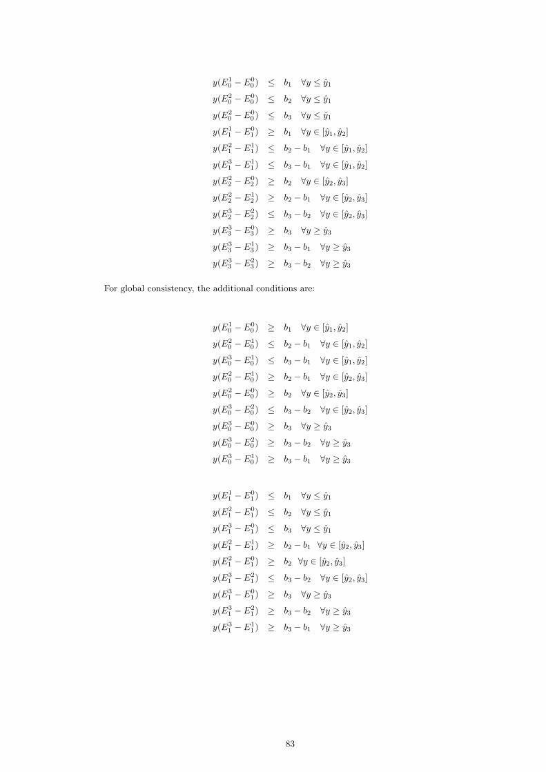
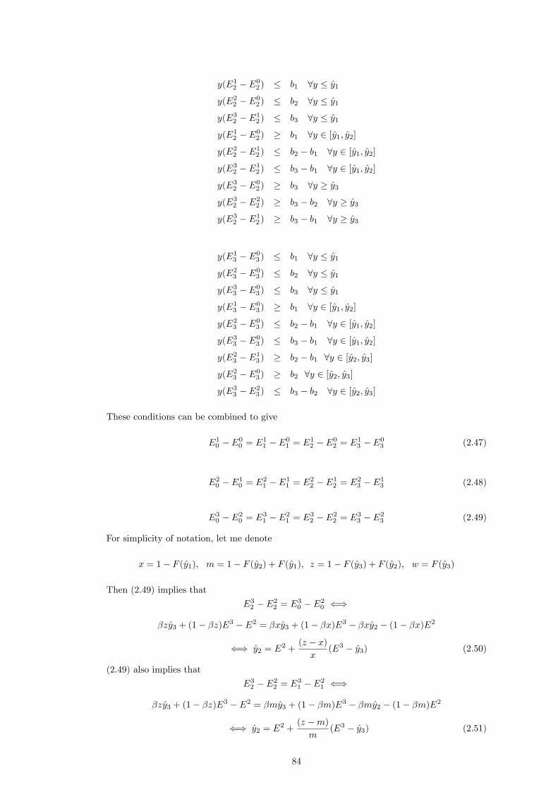
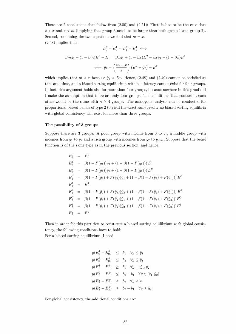
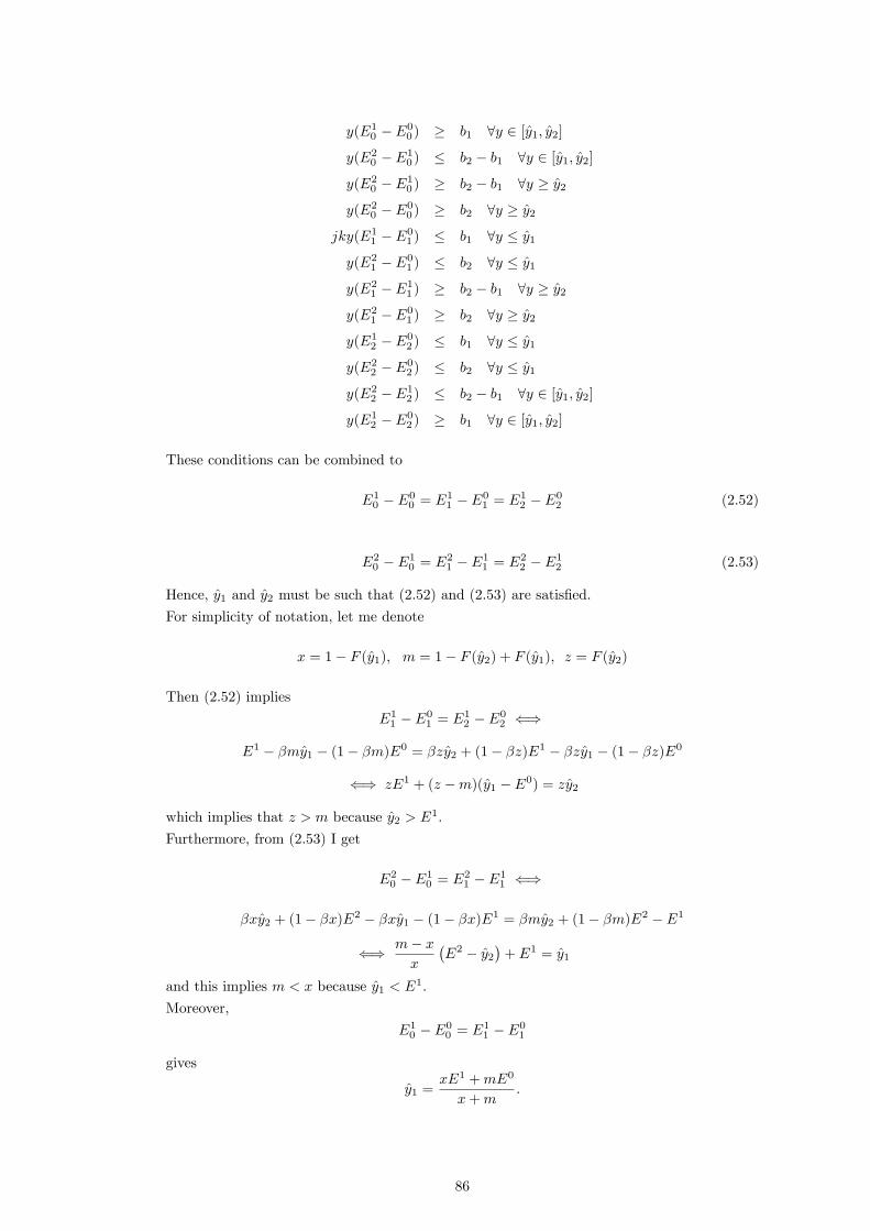
Finally, I want to thank my husband and best friend Stefan Rosenlechner for his immense
support, understanding and patience, for giving me a home (and a health insurance) and for
always bringing me back down to earth when I�m about to get lost in my ivory tower.
4
Abstract
This thesis consists of three papers that examine sorting and inequality.
In the �rst paper I present a model in which people sort into groups according to income and
as a result become biased about the shape of the income distribution. Their biased beliefs
in turn a¤ect who they choose to interact with, and hence there is a two-way interaction
between segregation and misperceptions about society. I show one possible application of this
novel framework to the question of income inequality and the demand for redistribution. I
demonstrate that under segregation an increase in income inequality can lead to a decline in
perceived inequality and therefore to a fall in people�s support for redistribution. I motivate my
main assumptions with empirical evidence from a small survey that I conducted via Amazon
Mechanical Turk.
In the second paper I develop a general model of how social segregation and beliefs interact.
Sorting decisions will be a¤ected by beliefs about society, but these beliefs about society are in
turn in�uenced by social interactions. In my model, people sort into social groups according to
income, but become biased about the income distribution once they interact only with their
own social circle. I de�ne �biased sorting equilibria�, which are stable partitions in which
people want to stay in their chosen group, despite their acquired misperceptions about the
other groups. I introduce a re�nement criterion � the consistency requirement � and �nd
necessary and su¢ cient conditions for existence and uniqueness of biased sorting equilibria.
In the third paper I present a model in which a monopolist o¤ers citizens the opportunity to
segregate into groups according to income. I focus initially on the case of two groups and show
that a monopolist with �xed costs of o¤ering the sorting technology will see pro�ts increase
as income inequality increases. I then analyze how the monopolist�s optimal group partition
varies with inequality and show that for a broad �eld of income distributions, monopolist
pro�ts increase with inequality, while at the same time total welfare of sorting given the
monopolist�s optimal schedule decreases. In the last section I examine how these �ndings
generalize if the monopolist doesn�t face costs of o¤ering the sorting technology and can
Most industrialized countries have seen a remarkable increase in income and wealth inequal-
ity over the past 35 to 40 years (see e.g. Piketty (2014)). At the same time, support for
redistributive policies hasn�t exhibited a comparable trend in the majority of these countries.
For instance, demand for redistribution as proxied by realized tax- and redistribution rates
has remained relatively constant or even decreased over the last two decades in the US (see
Piketty et al. (2014)). Of course there are many reasons - above all institutional ones - why
realized tax rates need not re�ect demand for redistribution well. However, also demand for
redistribution as measured by household surveys has not evolved in the same way as (income)
inequality (see Ashok et al. (2015) and Kenworthy and McCall (2008)). This is at odds
with standard Political Economy models, which predict that high rates of income inequality
trigger high demand for redistribution. For instance, in the baseline model of Meltzer and
Richard (1981) the redistribution rate that is determined by majority voting is increasing in
the di¤erence between median and mean income.
Rising income and wealth inequality have frequently been accompanied by an increase in
socio-economic segregation. Watson (2009) and Reardon and Bischo¤ (2011) demonstrate
that both income inequality and income segregation have risen sharply in the US between
1970 and 2000, especially in metropolitan areas. Often, middle-income neighbourhoods have
made way for both rich and poor communities, and segregation and the erosion of the middle
class have gone hand in hand.
In the present paper, I want to combine these observations with the �nding that people tend
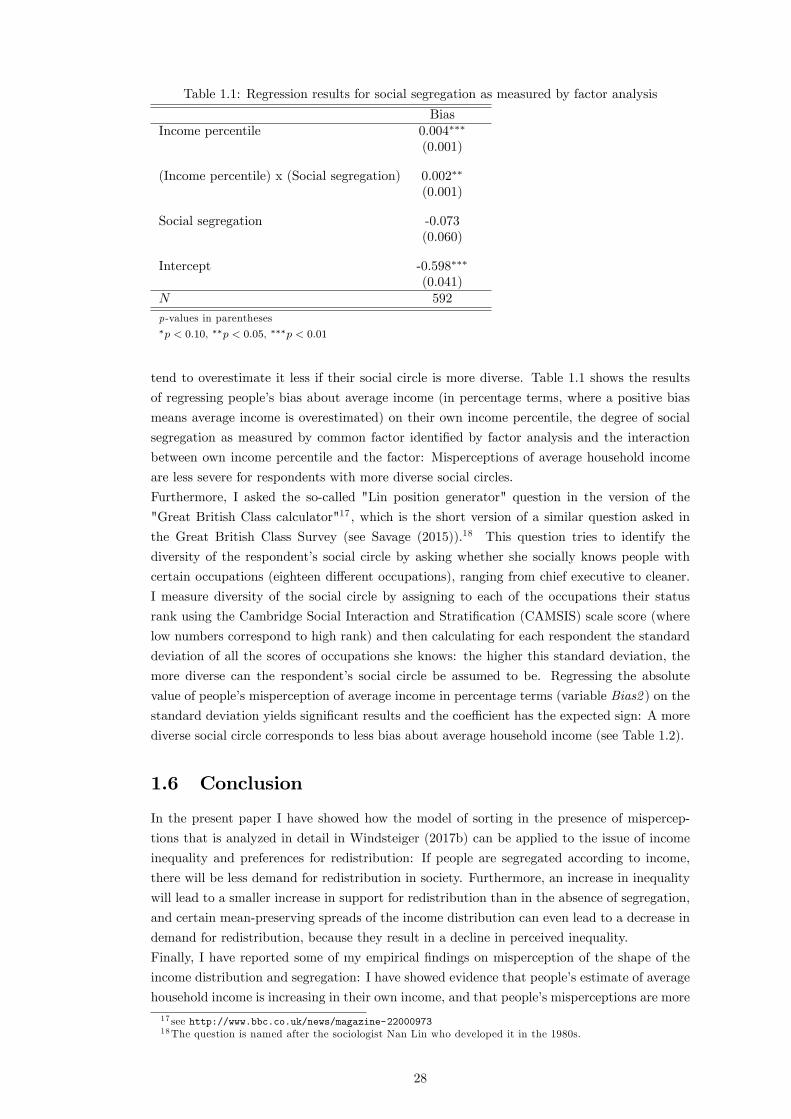
to misperceive the shape of the income distribution. Empirical studies in the US and Australia
�nd that people underestimate income and wealth inequality and wage di¤erentials (see e.g.
Norton and Ariely (2011) and Kiatpongsan and Norton (2014)) and I detect similar types
of misperception in my own survey conducted in the US via Amazon Mechanical Turk (see
Section 1.5).
Connecting all these pieces, I build a model that explains why the relationship between income
and wealth inequality and support for redistributive policies could be non-monotone in general:
In my model people are segregated according to income, and therefore interact mainly with
others who have similar incomes to themselves. As a result, they lose sight of the overall income
1 I thank Ronny Razin, Stephane Wolton, Thomas Piketty, Mike Savage, Matt Levy, Camille Landais, GilatLevy, Daniel Laurison, Dominik Hangartner, Stephan Maurer, Frank Cowell and the participants of the LSEMicroeconomic Theory Work in Progress Seminar for their helpful suggestions and comments.
10
distribution and become biased about the shape of the income distribution. Speci�cally, they
underestimate how di¤erent others are to themselves and therefore underestimate income
inequality.
This has an e¤ect on their support for redistributive policies: People in my model will in
general demand less redistribution than in a model without misperceptions. Furthermore, I
show that an increase in inequality will, in the presence of segregation and misperceptions,
always lead to a smaller increase in demand for redistribution than in a model where people
are unbiased, and that it can in certain circumstances even lead to a decrease in demand for
redistribution.
At the end of the paper I support my assumptions about misperceptions of the income dis-
tribution and segregation by presenting evidence from a survey that I conducted via Amazon
Mechanical Turk.
The rest of this paper is organized as follows: Section 1.2 discusses related literature. Section
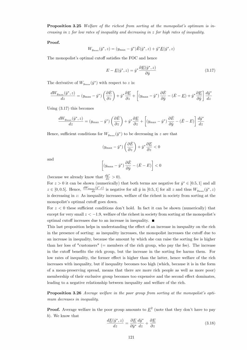
1.3 presents a theoretical model of economic sorting with misperceptions where people under-
estimate inequality and Section 1.4 applies this model to the issue of voting for redistribution.
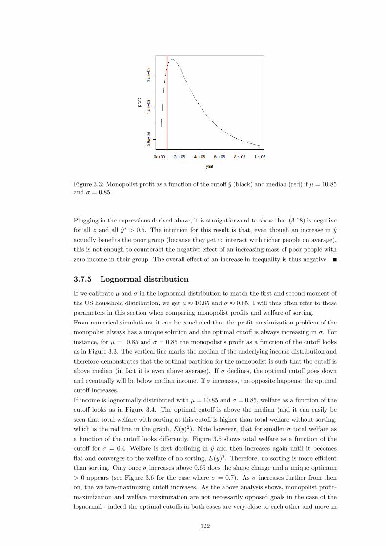
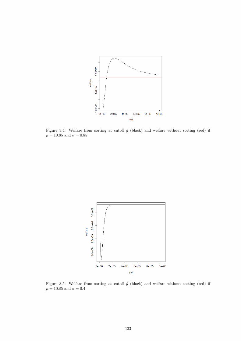
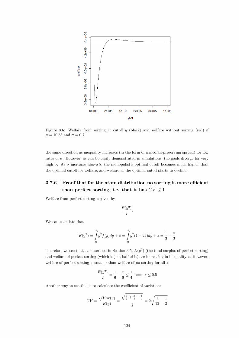
Section 1.5 presents suggestive empirical evidence on misperceptions about the shape of the
income distribution and on how socio-economic segregation and misperceptions of the income
distribution are related. Section 1.6 concludes.
1.2 Relation to existing literature
In Windsteiger (2017b) I present a general model in which beliefs about society and segregation
decisions interact to create an endogenous system of beliefs and social groups. For related
literature on segregation and belief formation see Windsteiger (2017b).
In the present paper I apply this general model to the situation of sorting according to income
and support for redistributive policies. Standard political economy models (see e.g. Meltzer
and Richard (1981)) predict that the demand for redistribution should be higher, the poorer
the median earner is relative to average income in society. However, studies comparing pre-
tax income inequality to redistribution rates in democracies, and hence trying to con�rm
the Meltzer-Richard Model empirically, deliver mixed results. Some papers do indeed �nd a
positive link between inequality and redistribution (see e.g. Borge and Rattsoe (2004), Meltzer
and Richard (1983) and Milanovic (2000)). However, others detect a negative relationship
(e.g. Georgiadis and Manning (2012) and Rodriguez (1999)) or no signi�cant link at all (e.g.
Kenworthy and McCall (2008) and Scervini (2012)).
There are many explanations for why a high degree of inequality might not be re�ected in
high realized redistribution rates in an economy: Bartels (2009) argues that the views of the
majority might be disregarded by political leaders due to successful lobbying of the �nancially
powerful. Moreover, poor people might participate in the political process to a lesser degree
than rich people, which might shift the identity of the median - decisive - voter (see e.g.
Larcinese (2005)). Finally, and importantly, people rarely get to vote directly on redistribution
rates. Instead, policital candidates o¤er platforms that take a position on a variety of issues,
and people might vote against their interest on the subject of redistribution if they consider
other issues to be more important (see Matakos and Xefteris (2016)).2 However, apart from
these factors, which a¤ect realized redistribution rates, it seems to be the case that even
the pure redistributive preferences of the population are not in line with what we might call
the "Meltzer-Richard-Hypothesis": that pre-tax inequality and the demand for redistribution
should be positively correlated, both across countries and over time (see e.g. Ashok et al.
2For a concise overview see Bonica et al. (2013).
11
(2015)).
In the Meltzer-Richard Model, people aim to maximize their own after-tax income and hence
their sole concern is their relative position in the income distribution as a direct predictor
of how much they would bene�t or lose from redistribution. More detailed models allow for
people�s preferences for redistribution to be in�uenced also by other factors, such as social
mobility, the overall degree of inequality in society or social status concerns (see e.g. Piketty
(1995), Benabou and Ok (2001), Alesina and Angeletos (2005) and Corneo and Gruener
(2000)). This can explain why the median voter�s relative position in the income distribution
is not necessarily a good predictor of a society�s demand for redistribution. However, also in
these more elaborate models it will be the case that if inequality increases (ceteris paribus), de-
mand for redistribution increases.3 Nevertheless, empirically we �nd that periods of increasing
inequality can be accompanied by stagnant or declining demand for redistribution.
The main contribution of my paper is that I show how my model of endogenous segregation
and belief formation can be used to explain low support for redistribution in societies where
inequality is high: As people interact only with people who have similar income to their
own, they misperceive the shape of the whole income distribution, and poor people (including
the median voter) underestimate how much they could gain from redistribution. Moreover,
I demonstrate that with endogenous segregation and beliefs, the relationship between redis-
tributive demand and inequality can be non-monotone - an increase in inequality can lead
to a decline in the demand for redistribution, because people, if they see only a select group
of society, might perceive that inequality has gone down due to the change in the income
distribution.
There is a growing empirical literature on people�s misperceptions of the income distribution.
Cruces et al. (2013) �nd that poor people in Buenos Aires overestimate their relative position
in the income distribution, while rich people underestimate it. They also show that this lowers
poor people�s demand for redistribution: when their biases are corrected, poor people�s demand
for redistribution increases. Importantly, they additionally show that (social resp. economic)
segregation a¤ects people�s misperceptions. Karadja et al. (2015) conduct a similar study for
Sweden and �nd that a majority of people there tend to underestimate their relative position.
Norton and Ariely (2011) and Norton et al. (2014) �nd that people in the US and Australia
tend to underestimate income and wealth inequality and Kiatpongsan and Norton (2014) �nd
that people underestimate pay di¤erences between di¤erent professions.
Kuziemko et al. (2015) perform a series of online experiments to analzye how information
about inequality and its evolution over time e¤ects people�s demand for redistribution. They
�nd that information has large e¤ects on whether people see inequality as a problem, but it
doesn�t move redistributive preferences a lot. The only exception is the estates tax: informing
people about the tiny share of inheritants who are subject to it drastically increases support
for it. The latter result seems to be due to a huge degree of ex-ante misinformation about the
estates tax and its incidence. They hypothesize that the relatively small e¤ect of information
on all other policy preferences might be due to the fact that becoming aware of the true extent
of inequality and its increase makes people less con�dent that the government is capable of
dealing with this issue, which is why respondents do not think redistributive policies can solve
the problem.
Concerning the theoretical model of sorting according to income outlined in Section 1.3, my
3A notable exception here is Corneo and Gruener (2000), where an increase in economic inequality canlead to a decrease in the preferred tax rate of the middle class due to status concerns - the signalling powerof wealth decreases more rapidly with the tax rate if income inequality is high and the middle class want toavoid mixing with the lower class. Note however that this depends crucially on the assumption that social andeconomic inequality move independently and that the middle class has a higher than average social status anda lower than average economic status.
12
paper is closely related to Levy and Razin (2015). They analyze preferences for redistribution
in the presence of costly income sorting. They identify simple conditions on the shape of the
income distribution such that a majority of the population (even people with income above
average) respectively a benevolent social planner prefer full redistribution (or no sorting)
to costly income sorting and they show that in both cases these conditions are satis�ed for
relatively equal income distributions. Hence, one implication of their model is that an increase
in income inequality can make sorting more desirable from a welfare perspective.
1.3 Sorting with misperceptions
In the following section I will introduce a theoretical model of sorting with misperceptions.
With the help of this framework I can then predict how groups in society will look like in
equilibrium and - because social interactions a¤ect beliefs - also what kind of misperceptions
people will have about the overall income distribution. The model below is a simpli�ed version
of a more general model presented in Windsteiger (2017b).
Let income y in an economy be distributed according to an income distribution F (y), on
the interval Y = [0; ymax] where ymax < 1: Assume furthermore that F (y) is continuousand strictly monotonic. As F (y) is an income distribution, I will also assume that F (y) is
positively skewed (meaning that the median income is smaller than the average income).
Suppose that an agent�s utility is increasing not only in her own income but also in the average
income of the people that she interacts with, which I will henceforth call her "reference group".
Speci�cally, a person with income yj gets utility Uj = yjE(yjy 2 Si), where Si is individualj�s reference group. If there is no economic segregation, everybody�s reference group is a
representative sample of the whole population, such that Uj = yjE(y): However, a person
with income yj can pay a fee b > 0 to join group Sb and get utility
yjE[yjy 2 Sb]� b
or refrain from paying b and get
yjE[yjy 2 S0]
where Sb is the set of incomes y of people who have paid b and S0 is the set of incomes y of
people who haven�t paid b. If people are unbiased about the overall income distribution, a
partition fS0; Sbg of Y and a sorting fee b constitute a sorting equilibrium i¤
yE[yjy 2 Sb]� b � yE[yjy 2 S0] 8y 2 S0 (1.1)
yE[yjy 2 Sb]� b � yE[yjy 2 S0] 8y 2 Sb (1.2)
In a sorting equilibrium people stay in the group that gives them the highest utility.
Suppose that people, once they are sorted into their group, become biased about average
income in the other group and hence about the overall income distribution. I will model a
group�s belief about the other group as resulting from a group belief "technology". Speci�cally,
I will assume that people�s biased perception of the other group�s average income can be
characterized by the continuous belief function
B : P! Y 4
where P is the space of all monotone partitions P = [S0; Sb] of Y . For the following analysis,
I will restrict my attention to monotone partitions, i.e. partitions P = [S0; Sb] of Y that
can be uniquely characterized by a cuto¤ y 2 Y (with the convention that S0 = [0; y) and
13
Sb = [y; ymax]), and I will henceforth call the people in S0 "the poor" and the people in Sb "the
rich". Without further assumptions, also non-monotone equilibria are possible if people have
misperceptions. In Appendix 1.7.1 I show that restricting the analysis to monotone partitions
is without loss of generality for the analysis that I conduct in this paper.4
I will assume that people are correct about average income in their own group. Furthermore,
I require misperceptions to be constant within groups, i.e. people who are in the same group
have the same misperception about the other group�s average (and thus misperceptions do
not depend on one�s own income directly, but on group membership).
The belief function B is thus a continuous function that maps all monotone partitions of Y
(and note that any monotone partition can be uniquely characterized by the cuto¤ y) into a
four-dimensional vector of beliefs
B(y) = (E(y); �Ep(y); Er(y);�E(y))
where the �rst two entries denote the poor group�s belief about average income in the poor
and the rich group respectively and the last two entries denote the rich group�s belief about
average income in the poor and the rich group. E(y) is the true average income in the poor
group, i.e. E(y) = E[yjy < y] and �E(y) is the correct average income in the rich group,�E(y) = E[yjy � y]: The poor�s belief about average income in the rich group is �Ep(y) and therich�s belief about average income in the poor group is Er(y):
Given the belief function B, I can de�ne the following:
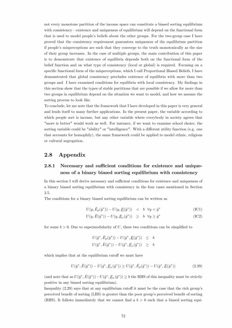
De�nition 1.1 A monotone partition of Y (characterized by an equilibrium cuto¤ y�) and a
sorting fee b > 0 constitute a biased sorting equilibrium i¤
y �Ep(y�)� b � yE(y�) 8y 2 [0; y�) (IC1)
y �E(y�)� b � yEr(y�) 8y 2 [y�; ymax] (IC2)
A biased sorting equilibrium is therefore a partition of Y that is "stable" given people�s
misperceptions about the other group. People compare the utility they obtain in their own
group to the utility they think they could obtain in the other group, given their misperceptions
about average income in the other group. In a biased sorting equilibrium people think that
they reach the highest possible level of utility in their own group and therefore they do not
want to move to the other group.
Assuming that people have misperceptions about average income in the other group creates
consistency issues: In a biased sorting equilibrium, people�s beliefs about the other group can
be inconsistent with what they see. A person in the poor group might wonder why a person
in the rich group �nds it worthwhile to pay b, given the poor person�s belief about average
income in the rich group. Similarly, a person in the rich group might - given the rich group�s
misperception about average income in the poor group - wonder why a certain person in the
poor group doesn�t want to join the rich group.
However, this inconsistency vanishes if I introduce what I call the consistency requirement. A
partition of society satis�es consistency if people�s beliefs about the other group are in line
with what they observe: People who are in the poor group think that the people who are in
the rich group are correct in doing so and vice versa. In Windsteiger (2017b), I explain this
requirement in detail.5 Formally, the consistency requirement translates to
4 I show that the re�nement that I introduce in this section (the consistency requirement), implies monotonic-ity.
5 If society is divided into more than two groups, the requirement can be stated in a global and a local form.In the case of two groups, the two notions coincide, which is why I will talk only about "consistency" in thepresent paper, without specifying whether it is local or global.
14
De�nition 1.2 A monotone partition of Y (characterized by a cuto¤ y) and a sorting fee b
satisfy consistency i¤
y �E(y))� b � yEr(y) 8y 2 [0; y) (CR1)
y �Ep(y)� b � yE(y)) 8y 2 [y; ymax] (CR2)
In words, condition (CR1) requires that a person in the rich group who looks at any person
with income y in the poor group thinks that this person cannot achieve higher utility by
switching to the rich group (and note that the person from the rich group evaluates person
y�s utility in the poor group given her own biased perception of average income in the poor
group, Er(y)). Condition (CR2) does the same for poor people�s belief about the rich group.
Without misperceptions, consistency is implicit in any sorting equilibrium. Because everybody
has the same (correct) understanding of average incomes in both groups, people cannot be
"puzzled" by other people�s choices - everybody evaluates everybody else�s utility in the same
way. It is only when people have incorrect perceptions of the other group that consistency
becomes a separate issue and is not implicit in the equilibrium de�nition. People can be happy
with their own choices (which means the partition constitutes a biased sorting equilibrium),
while at the same time not understanding other people�s choices (which means that consistency
is violated). Hence, it makes sense - as a re�nement to biased sorting equilibria - to de�ne
biased sorting equilibria which additionally satisfy consistency:
De�nition 1.3 A monotone partition of Y (characterized by an equilibrium cuto¤ y�) and a
sorting fee b > 0 constitute a biased sorting equilibrium with consistency i¤
y �Ep(y�)� b � yE(y�) 8y 2 [0; y�) (IC1)
y �E(y�)� b � yEr(y�) 8y 2 [y�; ymax] (IC2)
and
y �E(y�))� b � yEr(y�)) 8y 2 [0; y�) (CR1)
y �Ep(y�)� b � yE(y�) 8y 2 [y�; ymax] (CR2)
In Windsteiger (2017b) I show the following:
Corollary 1.1 A monotone partition of Y (characterized by a cuto¤ y�) and a sorting fee
b > 0 constitute a biased sorting equilibrium with consistency i¤
y �Ep(y�)� yE(y�) (1.3)
= y� �E(y�)� y�Er(y�)
= b
A biased sorting equilibrium with consistency is thus a partition where the perceived bene�t
of being in the rich group rather than the poor group (in terms of utility) of the person with
income at the equilibrium cuto¤ y� is regarded to be equally high by both groups. Note that
for a given equilibrium cuto¤ y� that satis�es (1.3), the corresponding sorting fee b is unique.
The equilibrium condition (1.3) restricts the set of belief functions which imply equilibrium
existence. In Windsteiger (2017b), I derive conditions on this function such that equilibrium
exists and is unique. For the remainder of this paper I want to focus on a particular type of
belief function: One where the poor underestimate average income in the rich group and the
15
rich overestimate average income in the poor group, and therefore both groups underestimate
income inequality. As I argue in the introduction, this is what empirical evidence shows. I will
present suggestive evidence for such misperceptions and how they are connected to segregation
in Section 1.5, where I explain a survey that I conducted myself via Amazon Mechanical Turk.
In Appendix 1.7.10 I examine the implications for the model if people have misperceptions of
the opposite type, where both groups overestimate inequality, and I compare the two types of
misperceptions in terms of welfare and pro�t of a monopolist who o¤ers the sorting technology
in Appendix 1.7.11 and 1.7.12, respectively.
1.3.1 Underestimating Inequality
Suppose the belief function B is such that the people in the poor group think that average
income in the rich group is
�Ep(y) = �(1� F (y))y + (1� �(1� F (y)) �E (1.4)
and the people in the rich group think that average income in the poor group is
Er(y) = F (y)y + (1� F (y))E. (1.5)
� 2 [0; 1] and 2 [0; 1] parameterize the "naivity" of agents and if � resp. is 0 agents haveno misperceptions. It is straightforward to see that �Ep(y) < �E(y) and Er(y) > E(y) for all
y 2 (0; ymax), i.e. the poor underestimate average income of the rich and the rich overestimateaverage income of the poor for any interior cuto¤. The functional form of �Ep(y) and Er(y)
implies that the misperceptions are more severe, the smaller the part of the distribution that
they can fully observe (which is F (y) for the poor group and 1 � F (y) for the rich group).Speci�cally, we have that
d( �E(y)� �Ep (y))
dy= ��(1� F (y)) < 0 8y 2 (0; ymax)
andd(Er(y)� E(y))
dy= F (y) > 0 8y 2 (0; ymax)
and therefore the misperceptions converge to the truth monotonically as y goes to 0 resp.
ymax.6
Misperceptions of this type could arise in the following way: As people live in their segregated
communities, they see mostly people who have income similar to their own (i.e. people from
their own group). They do meet people from the other group, but they are not aware that
most of the time they do not meet a representative sample of the other group (because they
are more likely to meet people from the other group who are close to the cuto¤). They see
the average income in their own group, but what matters for their sorting decision is also
the average income in the other group, which they do not see. Because they know y and the
overall range of y (i.e. that y ranges from 0 to ymax), they know that the average income of the
other group lies somewhere between the cuto¤ y and 0 resp. ymax. However, as they neglect
the fact that they often do not meet a representative sample of the other group and are rather
more likely to meet people very close to the cuto¤, the poor think that the average in the rich
6For the following analysis it is not necessary that the misperceptions are of exactly of the form (1.4) and(1.5) . For the results of the next section to hold, I need the misperceptions to be such that a binary biasedsorting equilibirum exists and is (ideally) unique. Su¢ cient conditions for this are stated in Windsteiger (2017).Furthermore, the equilibrium cuto¤ needs to be located above median income. In Appendix 1.7.2, I specifysu¢ cient conditions on the belief function to guarantee that there is a unique interior equilibrium cuto¤ abovethe median.
16
group is closer to their own average than it actually is, and the same holds for the rich when
thinking about the poor group�s average. In short, people below the cuto¤ underestimateaverage income in the rich group and people above the cuto¤ overestimate average incomein the poor group. This will lead both groups to underestimate the bene�ts of sorting: The
rich because they think the poor are less poor than they actually are, and the poor because
they think the rich are not as rich as they actually are.7
The functional form of the misperceptions as given by (1.4) and (1.5) is such that the su¢ cient
conditions for existence of a biased sorting equilibrium with consistency are satis�ed (see
Windsteiger (2017b)): �Ep(y) and Er(y) are continuous functions and each group is correct at
one of the endpoints, whereas the other group is maximally biased at that respective endpoint.
Furthermore, the misperceptions converge to the truth monotonically, and therefore there
exists a unique interior equilibrium cuto¤ if the utility function is linear. However, it is not
necessary to invoke these general conditions here, as existence and uniqueness can be proved
easily for the speci�c belief function that I use in the present paper:
The equilibrium cuto¤ with consistency can be calculated via the equilibrium condition
y�[ �E(y�)� Er(y�)] = y�[ �Ep(y�)� E(y�)] (1.6)
and note that the expressions on both sides also need to be equal to some b > 0, which rules
out y = 0 as an equilibrium cuto¤. Hence, any equilibrium cuto¤ y� must satisfy
�E(y�)� Er(y�) = �Ep(y�)� E(y�). (1.7)
Plugging in the functional form of the misperceptions, (1.4) and (1.5), and rearranging gives
�(1� F (y�))( �E(y�)� y�) = F (y�)(y� � E(y�))
and thus
y� =�(1� F (y�)) �E(y�) + F (y�)E(y�)
�(1� F (y�)) + F (y�)
which can be rewritten as
y� =a(1� F (y�)) �E(y�) + F (y�)E(y�)
a(1� F (y�)) + F (y�) (1.8)
where a = �= .8 An equiilibrium cuto¤ y� must thus be a �xed point of the function
h(y) =a(1� F (y�)) �E(y�) + F (y�)E(y�)
a(1� F (y�)) + F (y�) :
In Appendix 1.7.3 I prove that the function h(y) has a unique �xed point and hence that
7The speci�c form of misperception that I use in this paper can be microfounded in the following way:People in the poor group only sometimes encounter a representative sample of the rich (e.g. if they go to theopera, watch a royal wedding or shop in a fancy store) and the rest of the time encounter only rich peoplewho are very close to the cuto¤ (basically at y), maybe because they are parents of their kids�school friends(upper-middle class families sometimes prefer to send their kids to state schools). However, people are notaware of this and therefore estimate average income as if they were observing a representative sample of theother group. The particular functional form of the bias can arise if the frequency of meeting a representativesample of the other group depends on the size of the own group, F (y): This could be because "meeting arepresentative sample" does not actually require personal encounter but also comprises accounts from otherpeople who are in one�s own group. Then if people from di¤erent groups meet each other at a certain rate, thegroup with the bigger mass has a better understanding of the other group because people learn from others intheir own group.
8a > 0 if both types are assumed to be naive to some degree, i.e. � > 0 and > 0. If one of the groupswould be fully sophisticated, e.g. = 0, while the other group is naive, then consistency couldn�t be satis�edfor any (interior) cuto¤. If both groups are fully sophisticated, i.e. � = = 0, the model turns into a standardmodel of unbiased sorting.
17
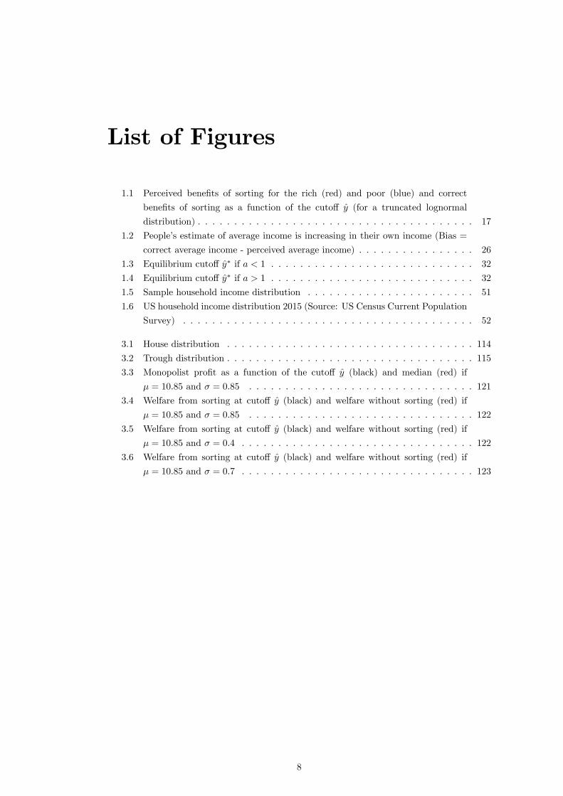
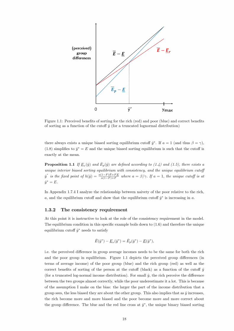
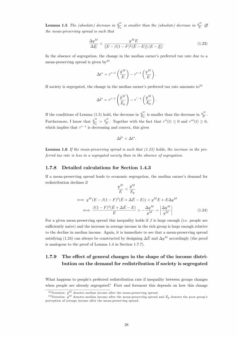
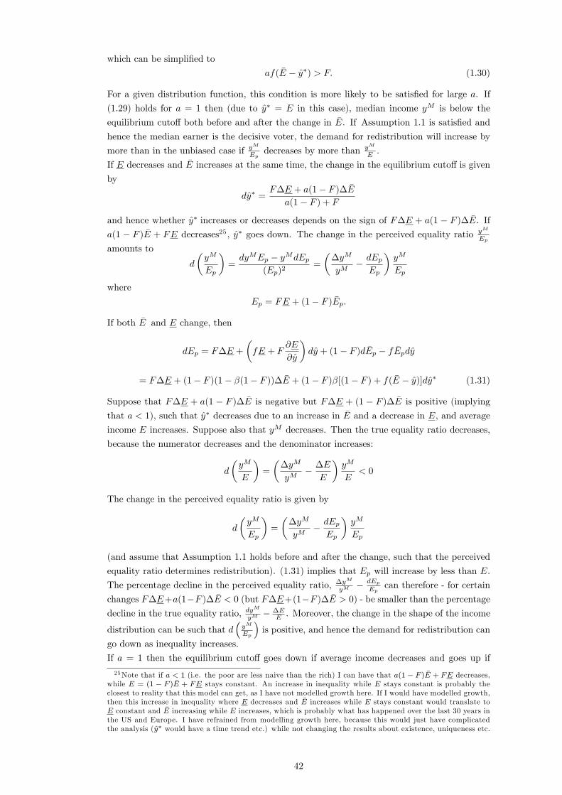
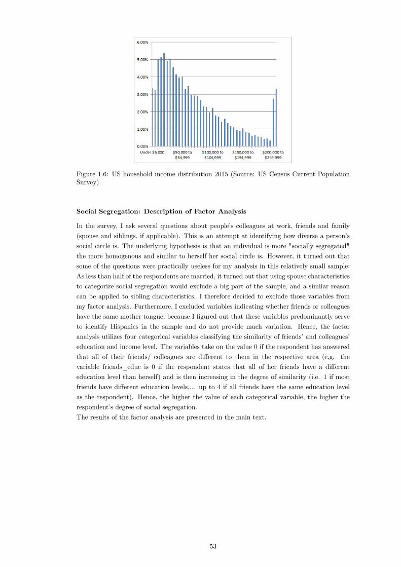
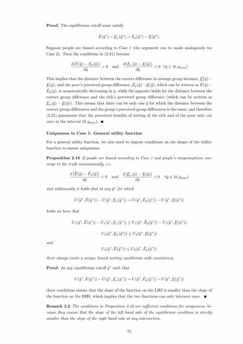
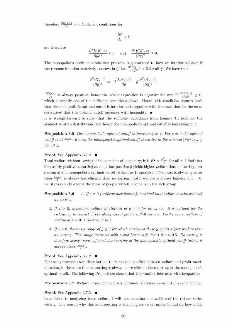
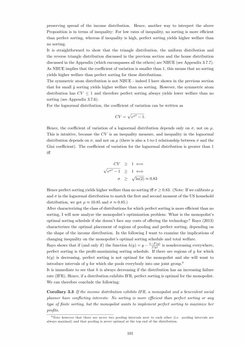
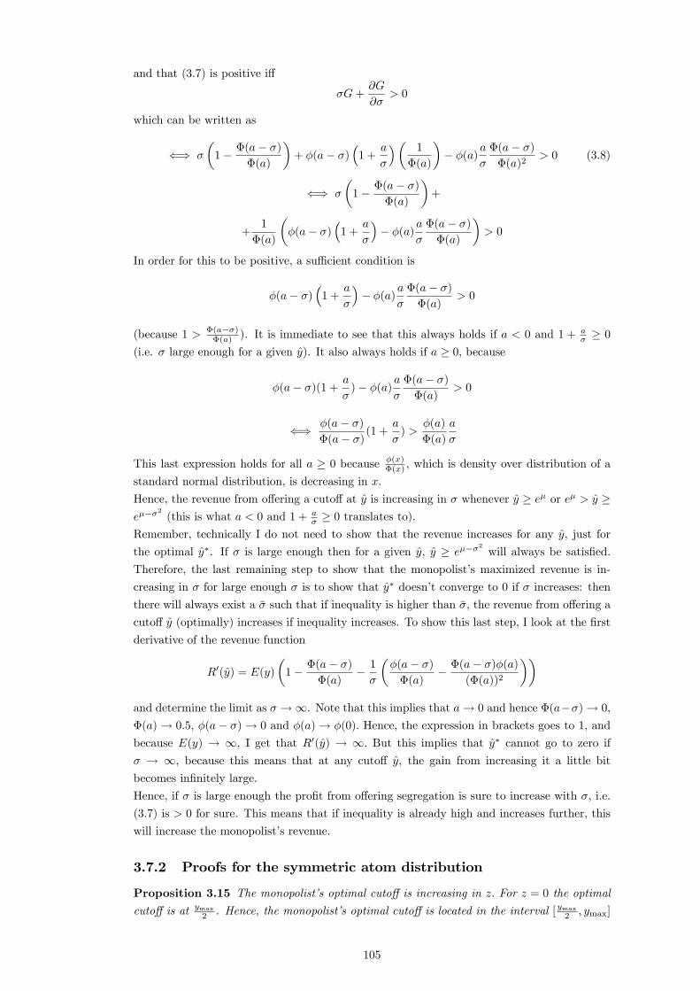
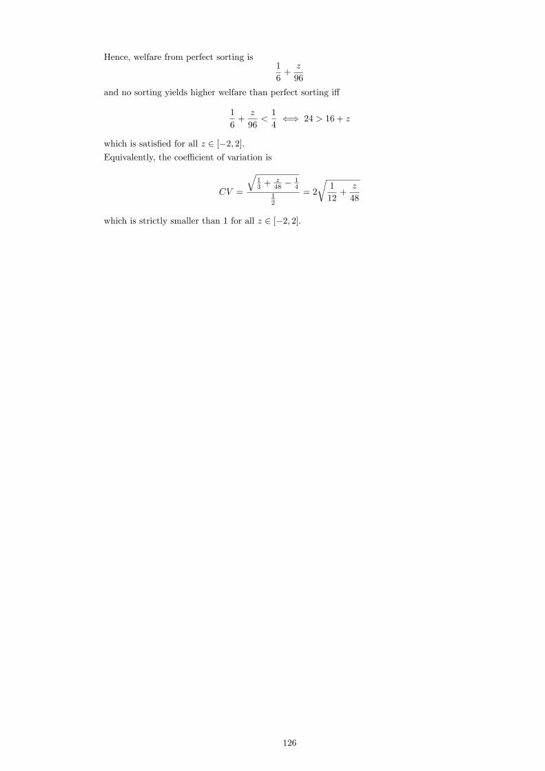
Figure 1.1: Perceived bene�ts of sorting for the rich (red) and poor (blue) and correct bene�tsof sorting as a function of the cuto¤ y (for a truncated lognormal distribution)
there always exists a unique biased sorting equilibrium cuto¤ y�. If a = 1 (and thus � = );
(1.8) simpli�es to y� = E and the unique biased sorting equilibrium is such that the cuto¤ is
exactly at the mean.
Proposition 1.1 If Er(y) and �Ep(y) are de�ned according to (1.4) and (1.5), there exists aunique interior biased sorting equilibrium with consistency, and the unique equilibrium cuto¤
y�is the �xed point of h(y) = a(1�F ) �E+FE
a(1�F )+F where a = �= : If a = 1; the unique cuto¤ is at
y� = E.
In Appendix 1.7.4 I analyze the relationship between naivety of the poor relative to the rich,
a, and the equilibrium cuto¤ and show that the equilibrium cuto¤ y� is increasing in a.
1.3.2 The consistency requirement
At this point it is instructive to look at the role of the consistency requirement in the model.
The equilibrium condition in this speci�c example boils down to (1.6) and therefore the unique
equilibrium cuto¤ y� needs to satisfy
�E(y�)� Er(y�) = �Ep(y�)� E(y�);
i.e. the perceived di¤erence in group average incomes needs to be the same for both the rich
and the poor group in equilibrium. Figure 1.1 depicts the perceived group di¤erences (in
terms of average income) of the poor group (blue) and the rich group (red) as well as the
correct bene�ts of sorting of the person at the cuto¤ (black) as a function of the cuto¤ y
(for a truncated log-normal income distribution). For small y, the rich perceive the di¤erence
between the two groups almost correctly, while the poor underestimate it a lot. This is because
of the assumption I make on the bias: the larger the part of the income distribution that a
group sees, the less biased they are about the other group. This also implies that as y increases,
the rich become more and more biased and the poor become more and more correct about
the group di¤erence. The blue and the red line cross at y�, the unique binary biased sorting
18
equilibrium with consistency, where both groups have the same perceived bene�ts of sorting.
As y increases beyond this point, the poor group starts to value sorting more than the rich
group.
For a sorting equilibrium without consistency, the only condition that needs to be satis�ed
is that the cuto¤ is such that everybody in the rich group prefers being in the rich group to
being in the poor group, while everybody in the poor group wants to stay in the poor group
for some sorting fee b > 0. In Figure 1.1, all cuto¤s y below y� would satisfy this condition -
if y 2 (0; y�); the marginal person in the rich group values being in the rich group more thanthe marginal person in the poor group, and therefore we would be able to �nd a sorting fee
b > 0 that the rich are willing to pay, while it doesn�t seem worthwhile for the poor to do so.
Hence, all y 2 (0; y�] are binary biased sorting equilibria. Meanwhile, none of the y above y�
can be biased sorting equilibria, because the marginal person in the poor group would always
be willing to pay more to join the rich group than the marginal person in the rich group, and
thus no b > 0 could be found that separates the rich from the poor. Note however, that all
y 2 (0; y�), while constituting biased sorting equilibrium cuto¤s, fail to satisfy the consistency
requirement: Depending on the sorting fee (and note that the sorting fee is not unique if
y 2 (0; y�), any b between y( �Ep � E) and y( �E � Er) would work), either the people in thepoor group would not understand why people at the bottom of the rich group want to pay b
to be part of the rich group (because for the poor, being in the rich group is worth less), or
the rich would wonder why people at the top of the poor group don�t want to join their group,
or both happens at the same time (if b is neither y( �Ep �E) nor y( �E �Er) but somewhere inbetween).
In the speci�c case analyzed here, the consistency requirement selects a unique equilibrium
out of the range of sorting equilibria. This is because the misperceptions converge to the truth
monotonically, which implies that the blue line approaches the black line monotonically as
the cuto¤ increases, while the red line approaches the black line monotonically as y decreases.
Therefore, the two lines can only cut once. If the misperceptions were not monotone, the
distance between the black line and the blue resp. red line could be non-monotone, and
therefore the blue and the red line could intersect several times. Each of those intersections
would then constitute a biased sorting equilibrium with consistency. Consistency alone is not
enough to guarantee uniqueness. Consistency and monotonicity of the misperceptions together
do the job.
Another way to interpret the consistency requirement is a re�nement to "no-learning parti-
tions". If a partition satis�es consistency, then people never come across anything that goes
against their beliefs and surprises them, therefore they have no impulse to modify their beliefs
or their actions in any way.
I do not model any form of learning in this paper. I also do not make any assumptions about
what happens if people encounter other people, whose choices they do not understand. One
possibility is that people just assume that the others are wrong if they are puzzled by their
choices, and do not modify their own beliefs or actions. Another possibility is that they start
to question their own beliefs about the other groups and maybe try to update them, based
on choices of other people that they observe. Alternatively, they might even experiment and
join another group to learn about average income in that group. The consistency requirement
restricts the set of biased sorting equilibria to those partitions where neither of the above
happens, because people are simply not puzzled by anybody else�s choices. In that sense,
the consistency requirement can be viewed as a stability re�nement: consistent equilibrium
partitions are stable with respect to learning, experimenting or updating. Because what they
see is consistent with their beliefs about the world, people have no incentives to question or
change their beliefs, and thus the partition is stable irrespective of what they would do if they
19
would encounter anything that is at odds with their beliefs.
1.4 Voting for Redistribution
Economic segregation can exacerbate inequalities in various ways. Schooling is one prominent
example: If children living in a uent areas get better education than children from poor
neighbourhoods because their local schools are of a better standard due to high local invest-
ment, income inequality in the next generation will be ampli�ed. This e¤ect is speci�cally
pronounced in the United States, where school choice is linked to neighbourhood (see e.g.
Chetty et al. (2014)). Moreover, having class mates from rich and in�uential families might
not only have the direct e¤ect on education via better quality of schooling, but might also
yield bene�ts later in life through social connections that lead to better jobs and opportunities
(see e.g. Savage (2015)).
In this section, I demonstrate that there might be another channel through which segregation
can a¤ect economic inequality: Economic segregation, if it leads to misperceptions of the
income distribution, can have signi�cant consequences for support for redistribution in society,
and hence for (post-tax and post-redistribution) income inequality. I show that segregation
leads poor people to underestimate what they can gain from redistribution and therefore to
show less support for redistribution than if they would have perfect knowledge of the income
distribution. Moreover, an increase in inequality (in the form of a mean-preserving spread
of the income distribution) always leads to a smaller increase in perceived inequality and
therefore in the demand for redistribution than if people were unbiased. The reason for this is
that people with income below average fully observe the fall of low incomes, but do not fully
see the o¤setting increase of high incomes. Therefore, they think that average income has
decreased. But because people�s gains from redistribution depend positively on the di¤erence
between their own income and (perceived) average income, and both decrease if people are
biased, demand for redistribution increases less than if people are unbiased and know that
average income hasn�t changed. I show that the increase in inequality can even be such that
perceived inequality declines and therefore people�s support for redistribution falls.
In the following analysis, I continue to use the functional forms of �Ep(y) and Er(y) as speci�ed
in (1.4) and (1.5), because this enables me to derive precise results. However, the general
�avour of those results would not change if more general speci�cations of �Ep(y) and Er(y)
were used that satisfy the conditions for existence of a unique equilibrium above the median,
given in Appendix 1.7.2.
1.4.1 Inequality and the demand for redistribution
Suppose that everybody in the economy has to pay a proportional tax t and the government
redistributes the proceeds equally among all its citizens afterwards. Hence, a person with
pre-tax income of yi has after-tax and after-redistribution income
(1� t)yi + �(t)E;
where the function �(t) � t accounts for the fact that there is a deadweight loss of taxation.(And let �(:) be such that �(t) > 0 8t 2 (0; 1); �(0) = 0; � 00(t) � 0; �(1) = 0; � 000(t) � 0 [thisguarantees that � 0(t) is convex and hence also � 0�1 is convex, given that � 0 is decreasing]).
Suppose furthermore that people vote to decide on the tax rate, and suppose that they care
only about their own post-tax income.
Meltzer and Richard (1981) have examined the relationship between inequality and the demand
20
for redistribution in this model: If people are unbiased about the income distribution, when
voting for the redistribution rate a person with income yi will simply choose the tax rate t
that maximizes her post-tax income
(1� t)yi + �(t)E.
As preferences are single-peaked in this case, the tax rate determined by majority voting will
be the median earner�s optimal tax rate given by
� 0(t�) =yM
E
if yM
E � 1 and t� = 0 otherwise. As � 0(t) is decreasing in t, the decisive voter�s optimal taxrate t� is decreasing in the ratio between median and average income.
The ratio yM
E can be regarded as an, albeit rudimentary, measure of the degree of income
equality in society. If the ratio is small, this means the di¤erence between median and mean
income is large and the income distribution has a large positive skew with a majority of people
earning income below average and a few very rich people. Therefore, income equality is low
and the demand for redistribution will be high in that case. If, on the other hand, the income
distribution is almost symmetric, with most people being middle-class and only a few at the
bottom and the top of the distribution, the equality ratio yM
E will be large (i.e. close to 1),
and demand for redistribution will be low.
To analyze people�s preferences for redistribution if they are biased, I need to establish what
their perception of average income is: If people would correctly perceive both average income
in their group and average income in the other group, they could simply calculate overall
average income via the formula
E = F (y)E(y) + (1� F (y)) �E(y)
for any cuto¤ y.9 However, if there is economic segregation and people are biased, then people
misperceive average income in the other group, and hence they mis-estimate overall average
income. Speci�cally, poor people think that average income is
Ep(y) = F (y)E(y) + (1� F (y)) �Ep(y) < E.
Because they underestimate average income in the rich group,
�Ep(y) < �E(y),
they end up underestimating overall average income. Analogously, rich people overestimate
average income,
Er(y) = F (y)Er(y) + (1� F (y)) �E(y) > E.
Let me for simplicity of exposition assume henceforth that rich and poor people are equally
naive, i.e. � = ,10 and remember that in this case the equilibrium cuto¤ will always be at
average income E. This implies that the median earner is in the poor group (because the
9Note that I assume that people know the relative size of their respective group, i.e. they know F (y) and1 � F (y). They also know the range of the distribution and where the cuto¤ lies. They only misperceive theshape of the distribution function in the other group. With the type of bias that I examine here, their perceivedincome distribution in the other group is more skewed towards y compared to the actual distribution.10The analysis can be done in a similar way for the general case of � 6= .
21
income distribution is positively skewed) and her preferred tax rate is given by
� 0(~t�) =yM
Ep(E)(or ~t� = 0 if Ep(E) < yM ).
Ep is smaller than E, hence the median earner�s perceived degree of equality as measured
by yM
Ep(E)is higher than without segregation. Therefore, her optimal tax rate is lower in the
presence of economic segregation.
Lemma 1.1 In the model with segregation and misperceptions the median earner�s preferredtax rate is lower compared to the model without misperceptions.
For the remainder of this paper, I will assume that the following condition on the income
distribution and people�s naivity holds:
Assumption 1.1 The distance between median and mean income is su¢ ciently high, suchthat
E
Er(E)� yM
Ep(E).
Remark 1.1 In Appendix 1.7.6 I show that EEr(E)
� yM
Ep(E)is guaranteed for misperceptions
(1.4) and (1.5) if
E � yM � ��E(E)� E(E)
4:
This condition holds if E�yM is large enough compared to �E(E)�E(E), i.e. if the distributionis positively skewed but there is not too much mass at the tails of the distribution, and if � is
small, i.e. people are not too biased.11
Lemma 1.2 If Assumption 1.7.6 holds, the median earner is the decisive voter.
The preferred tax rate of the poorest person in the rich group (i.e. the person earning average
income E) is given by
� 0(t) =E
Er(E):
If the distance between median and mean income is su¢ ciently high, such that Assumption
1.1 holds, then this person will demand a lower tax rate than the median earner, and hence
the median earner will be the decisive voter. As the median earner wants less redistribution
than in the unbiased case, the tax rate selected by majority voting will be lower and therefore
demand for redistribution in this segregated society will be lower than in a society without
segregation and misperceptions.
Proposition 1.2 The tax rate selected by majority voting in a segregated society where peoplemisperceive the shape of the income distribution as described above is lower than in a society
without segregation and misperception of the income distribution.
Proof. See above.
1.4.2 The e¤ect of changing inequality on demand for redistribution
In the following section I analyze what happens to people�s (mis)perceptions and the support
for redistribution in a segregated society if income inequality increases and how the e¤ects11Assumption 1.1 holds for positively skewed income distributions that look like actual income distributions
that we observe in the real world, for example it holds for a truncated lognormal (on (0; 108) ) with � = 10:85and � = 0:85 (the US household income distribution can be approximated by this function), and equally for ascaled down version of it, a truncated lognormal on (0; 10) with � = 0 and � = 0:85 (both times � = 0:1).
22
di¤er compared to a society without segregation. When analyzing the e¤ect of an increase in
inequality, it is important to clearly specify the exact form of this increase in inequality. Some
changes in the shape of the income distribution are such that it cannot even be unequivocally
decided whether they lead to an increase or decrease in inequality - di¤erent measures of
inequality might yield di¤erent results. However, any mean-preserving spread of the income
distribution always implies an increase in inequality, irrespective of the measure that is used,
because it can be decomposed into (potentially in�nitely many) transfers between rich and
poor where money is transferred from a relatively poor to a relatively rich person. It therefore
increases all measures of inequality that respect the principle of transfers, such as the Gini
coe¢ cient or the Theil index (see also Cowell (2000) and Dalton (1920)).12 Hence, I will focus
on the e¤ect of a mean-preserving spread of the income distribution on group formation and
demand for redistribution.
For simplicity, I require the mean-preserving spread to be such that the mass of people below
and above the mean remain the same, but mass shifts from the middle towards the endpoints
of the distribution, such that median income declines.13 Speci�cally, I will analyze the e¤ect
of what I call a monotone mean-preserving spread of the income distribution, which is such
that �E(y) increases and E(y) decreases for any cuto¤ y (see Windsteiger (2017c)).14 I will also
require that the mean-preserving spread is such that F (E) remains unchanged, and I require
Assumption 1.1 to hold before and after the change in inequality. As this implies that the
median earner is always the median voter, I will use these two expressions interchangeably.
In the absence of segregation and misperceptions, the median voter�s support for redistribution
increases due to a mean-preserving spread of the above described form, because median income
declines relative to average income and hence the equality ratio yM
E decreases,
�
�yM
E
�=�yM
E=�yM
yMyM
E;
i.e. the percentage change in yM
E is �yM
yM(where �yM < 0). This means that demand for
redistribution, given by
� 0(t�) =
�yM
E
�;
increases. The increase in the median voter�s optimal tax rate t� is
�t� = � 0�1�yM +�yM
E
�� � 0�1
�yM
E
�:
In a segregated society, where people misperceive the shape of the income distribution, the
e¤ect of an increase in inequality on the support for redistribution depends on its impact on
the location of the equilibrium cuto¤ y�, because this determines people�s beliefs about the
other group�s average income. Recall that the equilibrium cuto¤ y� is the �xed point of the
function
h(y) =a(1� F (y�)) �E(y�) + F (y�)E(y�)
a(1� F (y�)) + F (y�) :
As described in Section 1.3.1, h(y) has a unique �xed point, which is at average income E if
a = 1. Hence, the position of the equilibrium cuto¤ does not change due to a mean-preserving
spread if a = 1.
12 In the income and wealth inequality literature, an inequality measure is generally required to satisfy fourproperties: anonymity, scale independence, population independence and the principle of transfers. For anextensive discussion of di¤erent inequality measures see Cowell (2000).13This implies that the distance between mean and median income increases.14Such a mean-preserving spread can always be constructed if the initial distribution is strictly monotonic.
The easiest way is to take mass from the middle of the distribution and add it to the endpoints 0 and ymax(in such a way that average income doesn�t change).
23
What happens to perceived inequality and the demand for redistribution? As I explained in
the previous section, if people are biased due to segregation, the median voter�s optimal tax
rate ~t� is characterized by the equation
� 0(~t�) =
�yM
Ep(E)
�where ~t� < t� (because Ep < E) - the median earner�s preferred tax rate is lower under
segregation because perceived equality yM
Epis higher. While average income E does not change
due to a mean-preserving spread, I show in Appendix 1.7.7 that average perceived income of
the poor, Ep, declines. The poor feel that average income declines because they experience
the decline of average income in their own group fully, but only partially take note of the
compensating increase in average income among the rich. Hence, they think that society as a
whole has become poorer. As a result, the change in the perceived equality ratio yM
Epamounts
to
�
�yM
Ep
�=�yMEp � yM�Ep
(Ep)2 =
��yM
yM� �Ep
Ep
�yM
Ep
and thus the percentage decrease in yM
Epis �yM
yM� �Ep
Ep, which is smaller (in absolute terms)
than the percentage decrease of yM
E in the unbiased case, because �EpEp
< 0.
Proposition 1.3 If society is segregated, an increase in inequality (in the form of a monotonemean-preserving spread that keeps F (E) constant) always leads to a smaller percentage increase
in the median voter�s perceived inequality than in the absence of segregation and misperception.
Moreover, in Appendix 1.7.7 I demonstrate that one can always construct a mean-preserving
spread that leads the median voter to believe that society has become more rather than less
equal, i.e. that inequality has decreased rather than increased.
Proposition 1.4 There exists an increase in inequality that causes a decrease of the medianearner�s perceived degree of inequality under segregation.
The intuition for Proposition 1.4 is that, unlike in the non-segregated case, the median voter�s
perceived equality ratio yM
Epcan increase due to a mean preserving spread if people are biased,
because both yM and Ep decline. If the mean-preserving spread is such that the median
voter�s perceived degree of inequality decreases, as in Proposition 1.4, then also the median
voter�s demand for redistribution (i.e. her preferred tax rate) must necessarily decrease.
Corollary 1.2 There always exists an increase in inequality such that the tax rate determinedby majority voting decreases under segregation.
In Appendix 1.7.7, I derive the condition on the mean-preserving spread that guarantees
Proposition 1.4. As I explain above, this condition must ensure that the decline in Ep is
larger than the decline in yM . I also derive a weaker condition on the mean-preserving spread
that guarantees that even if perceived inequality does not decrease, demand for redistribution
increases less under segregation than without segregation. The step-by-step calculations in
Appendix 1.7.7 can be summarized as follows: If perceived equality decreases due to a mean-
preserving spread under segregation, the fact that the percentage decrease in perceived equality
is smaller if society is segregated is not enough to guarantee that also the increase in demand for
redistribution will be smaller than without segregation. There are two reasons for this: First,
as perceived equality is higher to start with under segregation, a smaller percentage decrease
does not automatically imply a smaller absolute decrease than in the absence of segregation.
Second, even if the decrease in perceived equality is lower also in absolute terms, it is not clear
24
whether the increase in demand for redistribution will be lower as well: this depends on the
shape of the deadweight loss function �(:): However, it turns out that the assumption that � 0
is decreasing and convex is su¢ cient to ensure that demand for redistribution increases less
under segregation if the absolute decrease in perceived equality is smaller than in the absence
of segregation. The condition on the mean-preserving spread that guarantees that demand
for redistribution under segregation increases by less if inequality increases compared to a
situation without segregation is weaker than the condition that is needed for Proposition 1.4.
In Appendix 1.7.9, I describe how more general changes in the shape of the income distribution
a¤ect demand for redistribution if society is segregated.
1.4.3 Inequality and the supply side of sorting
An alternative way to model the decline in perceived inequality after an increase in inequality
is to assume that there is no segregation in place before the change (because whoever o¤ers
the sorting technology doesn�t �nd it worthwhile) but then as inequality increases, o¤ering the
sorting technology becomes pro�table and therefore society becomes segregated (and people
become biased). I examine this in the following section for the case of a pro�t-maximizing
monopolist.
Suppose a pro�t-maximizing monopolist, who has a �xed cost c > 0 of o¤ering the sorting
technology, can decide whether or not to become active.15 Her pro�ts from o¤ering sorting
are
�(y�) = y�( �E(y�)� Er(y�))(1� F (y�))� c
Given that the equilibrium cuto¤ is at E and substituting for Er, this can be rewritten as
�(E) = E(E � E(E))[1� F (E)(1� F (E))]� c (1.9)
Suppose that initially the income distribution is such that
E(E � E(E))[1� F (E)(1� F (E))]� c < 0
and hence the monopolist prefers to stay out of the market. If inequality increases (again
in the sense of a monotone mean-preserving spread of the income distribution which leaves
F (E) constant), E � E increases. This means that if the increase in inequality is su¢ ciently
large, the pro�ts from o¤ering the sorting technology will become positive and the society
will become segregated. Thus, a large enough increase in inequality will lead to economic
segregation.
Lemma 1.3 Suppose that the income distribution is initially such that a pro�t maximizingmonopolist with �xed costs c > 0 does not �nd it pro�table to o¤er the sorting technology.
Then for any c > 0 there exists a mean-preserving spread of the income distribution such that
the monopolist�s pro�ts become positive.
Hence, I can compare the e¤ect of increasing inequality in the presence of segregation to its
e¤ect without taking into account segregation (and the resulting misperception). As in the
previous sections, I require Assumption 1.1 to be satis�ed after the increase in inequality, to
ensure that the median earner is the decisive voter.
If inequality increases and there is no segregation and people are unbiased, the median voter
will demand more redistribution than before the change, because median income yM is smaller
15 In Appendix 1.7.11, I show that the argument works in the same way if a welfare-maximizing social plannerdecides about o¤ering the sorting technology.
25
as a result of the mean-preserving spread, and hence also yM
E decreases:
�
�yM
E
�=�yM
E< 0
Therefore, the median earner�s demand for redistribution increases from
� 0�1�yM
E
�to
� 0�1�_yM
E
�;
where _yM = yM +�yM < yM is median income after the increase in inequality.
If the increase in inequality leads to economic segregation and hence causes people to be
biased, then the median voter�s demand for redistribution changes from
� 0�1�yM
E
�to
� 0�1�
_yM
Ep(E)
�;
where
Ep(E) = E � �(1� F (E))2( �E(E) + � �E(E)� E):
As Ep < E, the increase in the median voter�s demand for redistribution will be smaller than
in the absence of economic segregation.
Proposition 1.5 If an increase in inequality leads to economic segregation, the median voter�sdemand for redistribution will increase less than in the absence of segregation.
In Appendix 1.7.8 I show that I can always construct a mean preserving spread of the income
distribution such that demand for redistribution decreases under segregation.
Proposition 1.6 There exists an increase in inequality that causes economic segregation andleads to a decline in the tax rate determined by majority voting.
Apart from the mean-preserving spread described above there are also other types of increases
in inequality that would make it pro�table for the monopolist to o¤er one cuto¤. I demonstrate
in Appendix 1.7.5 that for the lognormal distribution an increase in the log-variance � (which
corresponds to an increase in the Gini-coe¢ cient but is a median-preserving instead of a
mean-preserving spread) also leads to an increase in the monopolist�s pro�ts (1.9).
1.5 Empirical Evidence
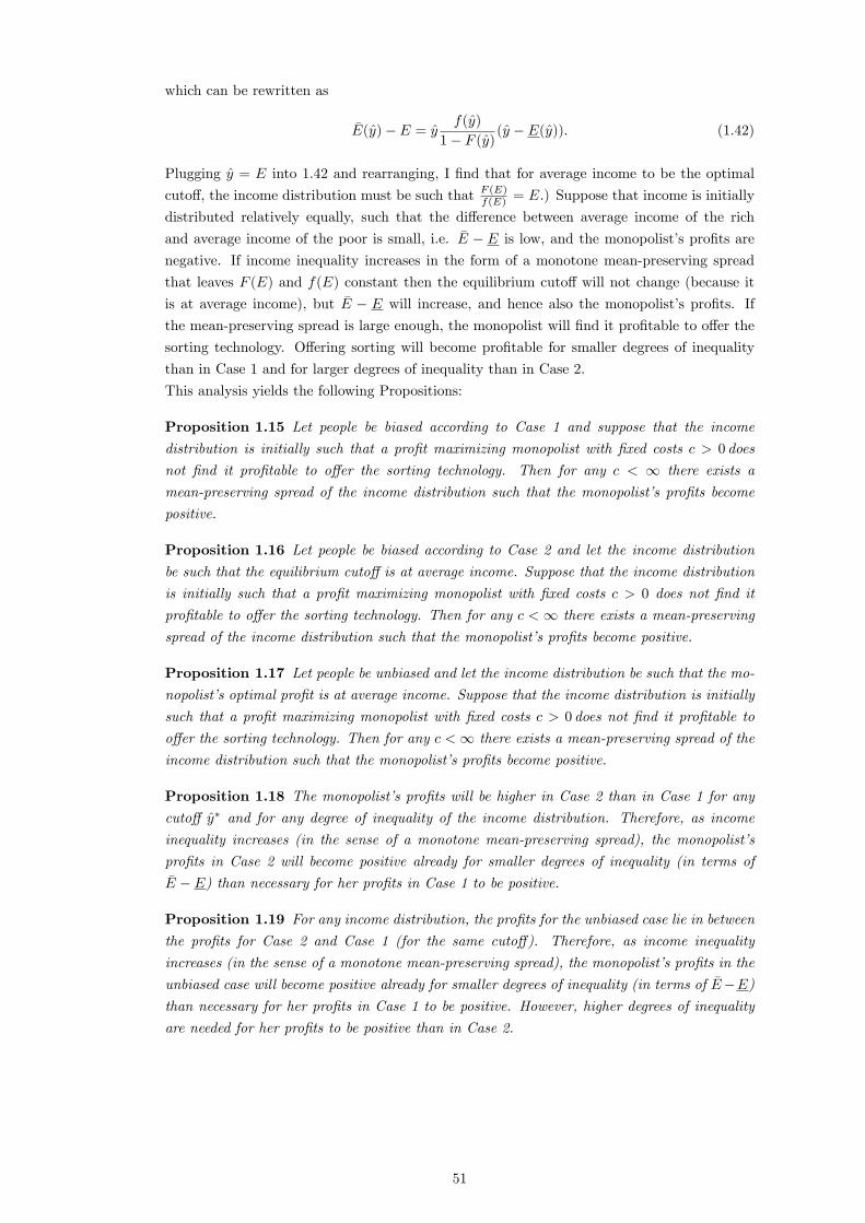
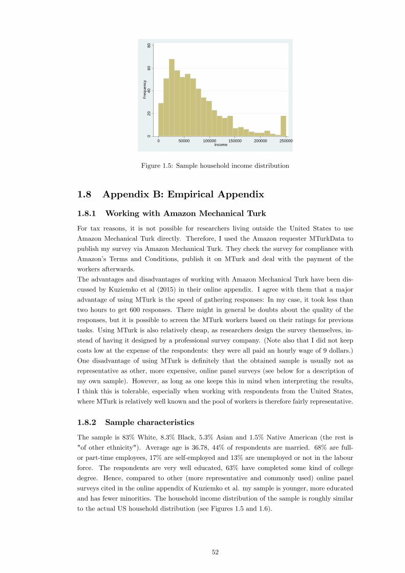
In February 2016, I conducted an online survey on 600 US citizens above the age of 18. The
survey was distributed via Amazon Mechanical Turk and the original questionnaire can be
accessed at https://lse.ut1.qualtrics.com/jfe/form/SV_eDLNkeGfQg2ycM5. A descrip-
tion of the sample (i.e. respondents�characteristics) can be found in Appendix 1.8.16 The
advantages and potential pitfalls of using Amazon Mechanical Turk in academic research have
been discussed by Kuziemko et al. (2015) in their Online Appendix. I summarize some of
their points and document my own experiences in Appendix 1.8.1.
16The data and all do-�les are available upon request.
My approach shows that modelling segregation and belief formation simultaneously can yield
interesting and unexpected results and o¤ers new perspectives on issues such as income inequal-
ity and redistribution. In the present paper, I have used the model to examine the implications
of segregation and biased beliefs on redistributive demand, but the general framework pre-
sented in Windsteiger (2017b) o¤ers itself to a wide set of applications related to segregation,
such as education policy and housing.
1.7 Appendix A: Theoretical Appendix
1.7.1 Consistency and monotonicity
Without imposing the consistency requirement, also non-monotone partitions can be biased
sorting equilibria (if the belief function is of a certain form): Suppose that y1 2 Sb and y2 2 S0with y1 < y2: In order for the partition [S0; Sb] to constitute a biased sorting equilibrium, it
must be the case that
y1Eb[S0] � y1E[Sb]� b
and
y2E[S0] � y2E0[Sb]� b:
(Notation: Ei[Sj ] is group Si�s belief about average income in Sj .) Combined, these two
conditions give
y2E0[Sb]� y2E[S0] � b � y1E[Sb]� y1Eb[S0]:
It is immediate to see that whether this inequality can hold depends on the belief function,
because even though y1 < y2; the misperceptions E0[Sb] and Eb[S0] could be de�ned in such
a way that
y1E[Sb]� y1Eb[S0] � y2E0[Sb]� y2E[S0]:
However, the consistency requirement rules out non-monotone equilibrium partitions for any
belief function.
Proposition 1.7 All biased sorting equilibria with consistency satisfy monotonicity.
29
Proof. Suppose a non-monotone equilibrium exists. Then it must be the case that there existy1 2 Sb and y2 2 S0 with y1 < y2: Then the IC constraint for y1 requires that
y1Eb[S0] � y1E[Sb]� b
and note that this implies that E[Sb]�Eb[S0] > 0. The consistency requirement additionallyrequires that
y2Eb[S0] � y2E[Sb]� b:
But these two conditions combined give
y1E[Sb]� y1Eb[S0] � y2E[Sb]� y2Eb[S0];
which cannot hold for any belief function B if y1 < y2, because as noted above E[Sb]�Eb[S0] >0.
1.7.2 Conditions for a unique equilibrium above the median withlinear utility
Proposition 1.8 (Windsteiger (2017b)) If the belief function is such that the rich overesti-mate average income of the poor group, and the poor underestimate average income of the rich
group, such that
Er(y) > E(y) 8y 2 [0; ymax) (1.10)
and�E(y) < �Ep(y) 8y 2 (0; ymax], (1.11)
a binary biased sorting equilibrium with consistency always exists. If additionally the severity
of the misperceptions is monotone in the cuto¤, i.e.
d( �E(y)� �Ep(y))
dy< 0 and
d(Er(y)� E(y))dy
> 0 8y 2 (0; ymax) (1.12)
the biased sorting equilibrium with consistency is unique.
Proof. Conditions (1.10) and (1.11) together with Assumption 1 and the fact that Er(y);E(y), �Ep(y) and �E(y) are continuous ensure existence. Condition (1.12) implies that people�s
misperceptions converge to the truth monotonically as y goes to 0 resp. ymax and hence there
will be a unique y� for which both groups have the same belief about the di¤erence in average
incomes (and thus about the bene�ts of sorting). For more explanations see Windsteiger
(2017b).
Proposition 1.9 If both groups underestimate inequality, su¢ cient conditions for a uniqueequilibrium cuto¤ y� above the median are conditions (1.10), (1.11) and (1.12) and additionally
�Ep(yM ) + Er(y
M ) < 2E:
Proof. The �rst three conditions guarantee existence and uniqueness (see above). Concerningthe last condition, note that if �E� �Ep is monotonically increasing and Er�E is monotonicallydecreasing in y, then
�Ep(y)� E(y) < �E(y)� Er(y)
30
for all y below the unique equilibrium cuto¤, and the inequality must hold in the other direction
above the unique equilibrium cuto¤. That implies
�Ep(y) + Er(y) <�E(y) + E(y)
for all y below the equilibrium cuto¤, and
�Ep(y) + Er(y) >�E(y) + E(y)
for all y above the equilibrium cuto¤. If the equilibrium should lie above the median, then at
the median it must be the case that
�Ep(yM ) + Er(y
M ) < �E(yM ) + E(yM );
because the median must be below the cuto¤. The fact that
E = (1� F (yM )) �E(yM ) + F (yM )E(yM ) =�E(yM ) + E(yM )
2
at the median proves the claim.
1.7.3 Analysis of the unique binary biased sorting equilibrium
As established in Section 1.3.1, any equilibrium cuto¤ is characterized by
y� =a(1� F (y�)) �E(y�) + F (y�)E(y�)
a(1� F (y�)) + F (y�) (1.13)
and hence it is the �xed point of
h(y) =a(1� F (y)) �E(y) + F (y)E(y)
a(1� F (y)) + F (y)
Therefore, the equilibrium cuto¤ is exactly where the 45 degree line cuts the function h. As
y� approaches 0, the left hand side of (1.13) becomes zero, while the right hand side becomes
h(0) = E, and hence larger than the left hand side. As y� approaches ymax, the opposite
happens: the left hand side becomes ymax, and thus larger than the right hand side, which
is again h(ymax) = E. Hence, because the expressions on both sides are continuous in y, we
know that there must be a y in (0; ymax) for which equality holds. This concludes the proof
that an equilibrium cuto¤ always exists in my model.
To ensure that there can only be one such intersection point, I can calculate
h0(y) =
" ��af(y) �E(y) + a(1� F (y))@ �E(y)@y + f(y)E(y) + F (y)@E(y)@y
�(a(1� F (y)) + F (y))
��a(1� F (y)) �E(y) + F (y)E(y)
�(�af(y) + f(y))
#(a(1� F (y)) + F (y))2
which can be simpli�ed to
h0(y) =(1� a)f(y)
(a(1� F (y)) + F (y))2�a(1� F (y))(y � �E(y)) + F (y)(y � E(y))
�:
This implies that h has a local extremum or saddle point y�� characterized by
a(1� F (y��))(y�� � �E(y��)) + F (y��)(y�� � E(y��)) = 0
31
or equivalently
y�� =a(1� F (y��)) �E(y��) + F (y��)E(y��)
a(1� F (y��)) + F (y��) (1.14)
This is exactly the equation that characterizes the equilibrium cuto¤ and the �xed point of
h, i.e. we �nd that y�� = y�. Whenever the 45 degree line cuts h it must therefore be where
the slope of h is 0: This means that at any intersection, the 45 degree line cuts h from below,
which implies that such an intersection can only happen once. It follows that h will have a
unique �xed point and the equilibrium cuto¤ is unique.
The �xed point of h characterized by (1.14) (or equivalently (1.13)) is a local maximum if
a > 1 and a local minimum if a < 1. This can be seen from noting that
h00(y) =(1� a)f 0(y)
(a(1� F (y)) + F (y))2�a(1� F (y))(y � �E(y)) + F (y)(y � E(y))
�+
(1� a)f(y)(a(1� F (y)) + F (y))
�2(1� a)2f2(y)
�a(1� F (y))(y � �E(y)) + F (y)(y � E(y))
�(a(1� F (y)) + F (y))3 :
At y� we know that
a(1� F (y�))(y� � �E(y�)) + F (y�)(y� � E(y�)) = 0
and thus the �rst and the third term drop out of the second derivative and we get
h00(y�) =(1� a)f(y�)
(a(1� F (y�)) + F (y�)) :
As this expression is negative for a larger than 1 and positive for a smaller than 1, y� is a local
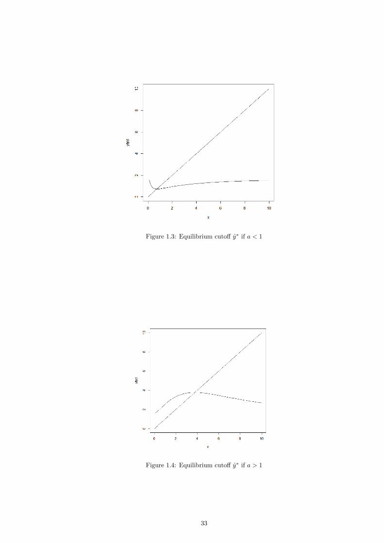
maximum if a > 1 and a local minimum at a < 1. Figures 1.3 and 1.4 depict the intersection
of h and the 45 degree line for a < 1 and a > 1 (where the underlying income distribution
is a truncated lognormal distribution). If a = 1 the problem becomes very simple, as the
expression for h reduces to
h(y) = E;
i.e. h is just a horizontal straight line at E and the unique equilibrium cuto¤ is at E.
1.7.4 The relationship between naivety and the equilibrium cuto¤ y�
As noted in Section 1.3.1, the equilibrium cuto¤ depends on the naivety of the rich and the
poor via a single parameter, � = a, which describes the severity of the poor�s naivety relative
to the rich�s. If a = 1 then both groups are "equally naive", if a > 1 then the poor are more
naive than the rich. Using the equilibrium condition
y� =a(1� F (y�)) �E(y�) + F (y�)E(y�)
a(1� F (y�)) + F (y�) ; (1.15)
I can investigate how y� changes with a:
(1� F (y�)) �E(y�)da+��af(y�) �E(y�) + a(1� F (y�))
�E(y�)� y�1� F (y�) f(y
�) + f(y�)E(y�) + F (y�)(y� � E(y�))F (y�)
f(y�)
�dy�
= (a(1� F (y�)) + F (y�) + y�(�af(y�) + f(y�)))dy� + (1� F (y�))y�da
da=(1� F (y�))( �E(y�)� y�)a(1� F (y�)) + F (y�) > 0 (1.16)
The equilibrium cuto¤ y� is increasing in the degree of naivety of the poor relative to the rich.
The higher a, the more the poor tend to underestimate the bene�ts of sorting (relative to the
rich) and hence the more they need to see of the whole distribution relative to the rich to have
the same perceived bene�ts of sorting as the rich.
As naivety goes to zero, what happens to the equilibrium cuto¤ depends on the speed of
convergence of � respectively : If � converges to zero faster than , a goes to zero and y�
goes to 0. If converges at a faster speed than �, a converges to in�nity and the equilibrium
cuto¤ goes to ymax.19
1.7.5 A median-preserving spread of the lognormal distribution andmonopolist pro�ts
Recall that the monopolist�s pro�ts from o¤ering one cuto¤ (which in equilibrium will be at
E if a = 1) can be written as
E(E � E)[1� F (E)(1� F (E))]� c
For the lognormal distribution, this becomes
� = E
24E0@1� �
�ln(E)��
� � ��
��ln(E)��
�
�1A 1� �� ln(E)� �
�
�+
��
�ln(E)� �
�
��2!35� cwhich can be simpli�ed to
� = E
"E
1�
1� ���2
����2
� !�1� �
��2
�+
h���2
�i2�#� c
= E2
2���2
�� 1
���2
� !�1� �
��2
�+
h���2
�i2�� c
because ln y = �+ �2 if y = E:
I �nd thatd�
d�= 2�E2
2���2
�� 1
���2
� !�1� �
��2
�+
h���2
�i2�
+E2
"�(�2 )
12
���2
� #�1� ���2
�+
h���2
�i2�
+E2
2���2
�� 1
���2
� ! ���2
�����2
�� 12
�As �
��2
�> 1
2 , all of the terms are positive and hence the monopolist�s pro�t always increases
if � increases.
Proposition 1.10 If income is lognormally distributed, an increase in inequality in the formof a median-preserving spread increases the monopolist�s revenues from o¤ering the sorting
19The best way to see the latter is to introduce the auxiliary parameter b = �in this case and rewrite h(y)
in terms of b.
34
technology.
1.7.6 Su¢ cient conditions for Assumption 1.1
yM
Ep� E
Er
() yM (FEr + (1� F ) �E) � E(FE + (1� F ) �Ep)
If � = , this can be simpli�ed to
�(yMF 2(E � E) + E(1� F )2( �E � E)) � E(E � yM )
Noting that
E � E = (1� F )( �E � E)
and�E � E = F ( �E � E)
I can further simplify to
�F (1� F )�FyM
E+ (1� F )
�( �E � E) � (E � yM )
Given that F (1� F ) < 0:25 (because yM < E) and yM
E < 1, I have that
�F (1� F )�FyM
E+ (1� F )
�( �E � E) < � (
�E � E)4
(1.17)
and it follows that
�( �E � E)
4� E � yM
is a su¢ cient condition foryM
Ep� E
Er
(in fact it is even a su¢ cient condition for yM
Ep< E
Er, given that inequality (1.17) is strict).
1.7.7 Detailed calculations for Section 1.4.2
Average income E does not change due to a mean-preserving spread and hence20
�E = F�E + (1� F )� �E = 0; (1.18)
Average perceived income of the poor, Ep, declines, because
�Ep = F�E + (1� F )� �Ep
and�Ep(y) = �(1� F )y + (1� �(1� F )) �E
which implies
� �Ep(E) = (1� �(1� F ))� �E < � �E (1.19)
20And note that I require the mean-preserving spread to be such that F (y�) = F (E) doesn�t change.
35
(as y = E doesn�t change). The change in yM
Epamounts to
�
�yM
Ep
�=�yMEp � yM�Ep
(Ep)2 =
��yM
yM� �Ep
Ep
�yM
Ep
and thus the percentage change in yM
Epis �yM
yM� �Ep
Ep, which is smaller (in absolute terms)
than the percentage change of yM
E in the unbiased case, because �EpEp
< 0. In the following I
show that if����EpEp
��� is large enough relative to ����yMyM
���, the median earner will even think thatinequality has decreased, i.e. the percentage change in yM
Ep(and hence also the absolute change
in yM
Ep) can be positive:
From (1.18) and (1.19) it follows that
�Ep(E) = �(1� F )� �E + (1� F )� �Ep(E) = ��(1� F )2� �E(E)
Furthermore,
Ep(E) = FE(E) + (1� F ) �Ep(E) = E � �(1� F )2( �E(E)� E)
and therefore
�EpEp
=��(1� F )2� �E
E � �(1� F )2( �E � E)=
�(1� F )F�EE � �(1� F )2( �E � E)
(using (1.18) again). Hence, I get
�yM
yM� �Ep
Ep> 0 () �yM
yM>
�(1� F )F�EE � �(1� F )2( �E � E)
() �yM
�E<
�yM (1� F )FE � �(1� F )2( �E � E)
(1.20)
(where both sides are positive). For a given �yM
�E this condition is more likely to be satis�ed
if � is large, because
@
@�
��
E � �(1� F )2( �E � E)
�=
E�E � �(1� F )2( �E � E)
�2 > 0and hence the RHS is increasing in �. Furthermore, (1�F (E))F (E) should not be too small,i.e. the income distribution cannot be too positively skewed, such that F (E) is not too far
above 0:5. Note however, that such a monotone mean-preserving spread can be constructed
for any given income distribution, by ensuring that �yM and �E are such that (1.20) holds.
To see this, note that we need to ensure that Assumption 1.1 is satis�ed before and after the
mean-preserving spread. A su¢ cient condition for this is that
�( �E(E)� E(E))
4� E � yM (1.21)
holds (see Section 1.7.6). If the mean-preserving spread would be such that �yM = 0 (i.e. all
the mass shifts around below and above the median, but the median stays the same), then
(1.20) would be satis�ed. If this mean-preserving spread is such that �E (and corresponding
� �E) are small enough (in absolute value) and therefore Assumption 1.1 still holds after the
change21 , this mean-preserving spread would lead to a decrease in demand for redistribution
21By continuity, such a mean-preserving spread can always be found because if (1.21) is satis�ed initially
36
(whereas in the unbiased case demand for redistribution would not change because neither
yM nor E has changed). Because all the expressions are continuous, it follows that we can
analogously construct a mean-preserving spread that satis�es (1.21) and has �yM > 0 (and
where thus demand for redistribution increases in the unbiased case, but decreases in the
presence of misperceptions). Hence, I can conclude that
Lemma 1.4 For any � > 0 there exists a mean-preserving spread of the income distributionsuch that an increase in inequality leads to a decrease in the median earner�s perceived degree
of inequality.
Now let me examine the absolute change of yM
E and yM
Ep: I want to derive su¢ cient conditions
for the absolute decrease in perceived equality to be smaller under segregation, i.e.
�
�yM
E
�< �
�yM
Ep
�(1.22)
(because both sides of this inequality are negative). Lemma 1.4 shows that I can always
construct a mean-preserving spread satisfying (1.20) such that perceived equality yM
Epincreases
under segregation (in which case inequality (1.22) trivially holds, because yM
E will always
decrease). However, less strong conditions can be derived in order for (1.22) to hold without
perceived inequality having to decrease:
�
�yM
E
�< �
�yM
Ep
�()
�yM
E<�yMEp � yM�Ep
(Ep)2 =
�yM
Ep� y
M�Ep
(Ep)2
() �yM
E<
�yM
E � �(1� F )2( �E � E)+
yM�(1� F )2� �E�E � �(1� F )2( �E � E)
�2() �yM
�1
E� 1
E � �(1� F )2( �E � E)
�<
yM�(1� F )2� �E�E � �(1� F )2( �E � E)
�2() �yM
yM
���(1� F )2( �E � E)
E(E � �(1� F )2( �E � E))
�<
�(1� F )2� �E�E � �(1� F )2( �E � E)
�2() �yM
yM
��( �E � E)
E
�<
� �E
E � �(1� F )2( �E � E)
() �yM
yM
��F ( �E � E)
E
�<
�F�E1�F
E � �(1� F )2( �E � E)
() ��yM
yM
�(1� F )( �E � E)
E
�<
��EE � �(1� F )2( �E � E)
() �yM
�E
�E � EE
�<
yM
E � �(1� F )2( �E � E)
() �yM
�E<
yME�E � �(1� F )2( �E � E)
�(E � E)
=yME
Ep(E � E)
For a given mean-preserving spread, this inequality is more likely to hold if � is large (such
that Ep is small relative to E). Note however, that it is always possible to construct a mean-
preserving spread that satis�es this inequality, by designing �yM and �E accordingly.
then yM
Epis strictly smaller than E
Er(see Section 1.7.6) and hence a small change in �E and E will still leave
yM
Ep� E
Er:
37
Lemma 1.5 The (absolute) decrease in yM
Epis smaller than the (absolute) decrease in yM
E i¤
the mean-preserving spread is such that
�yM
�E<
yME�E � �(1� F )2( �E � E)
�(E � E)
: (1.23)
In the absence of segregation, the change in the median earner�s preferred tax rate due to a
mean-preserving spread is given by22
�t� = � 0�1�_yM
E
�� � 0�1
�yM
E
�:
If society is segregated, the change in the median earner�s preferred tax rate amounts to23
�~t� = � 0�1
_yM
_Ep
!� �
0�1�yM
Ep
�:
If the conditions of Lemma (1.5) hold, the decrease in yM
Epis smaller than the decrease in yM
E .
Furthermore, I know that yM
Ep> yM
E . Together with the fact that �00(t) � 0 and � 000(t) � 0,
which implies that � 0�1 is decreasing and convex, this gives
�~t� < �t�:
Lemma 1.6 If the mean-preserving spread is such that (1.23) holds, the increase in the pre-ferred tax rate is less in a segregated society than in the absence of segregation.
1.7.8 Detailed calculations for Section 1.4.3
If a mean-preserving spread leads to economic segregation, the median earner�s demand for
redistribution declines ifyM
E<_yM
Ep
() yM (E � �(1� F )2( �E +� �E � E)) < yME + E�yM
() �(1� F )2( �E +� �E � E)E
> ��yM
yM=
�����yMyM���� (1.24)
For a given mean-preserving spread this inequality holds if � is large enough (i.e. people are
su¢ ciently naive) and the increase in average income in the rich group is large enough relative
to the decline in median income. Again, it is immediate to see that a mean-preserving spread
satisfying (1.24) can always be constructed by designing � �E and �yM accordingly (the proof
is analogous to the proof of Lemma 1.4 in Section 1.7.7).
1.7.9 The e¤ect of general changes in the shape of the income distri-bution on the demand for redistribution if society is segregated
What happens to people�s preferred redistribution rate if inequality between groups changes
when people are already segregated? First and foremost this depends on how this change
22Notation: _yM denotes median income after the mean-preserving spread.23Notation: _yM denotes median income after the mean-preserving spread and _Ep denotes the poor group�s
perception of average income after the mean-preserving spread.
38
a¤ects the equilibrium cuto¤ y�. Recall that the equilibrium cuto¤ is given by
y� =a(1� F (y�)) �E (y�) + F (y�)E (y�)
a(1� F (y�)) + F (y�) ; (1.25)
i.e. y� is the �xed point of the function
h(y) =a(1� F (y)) �E(y) + F (y)E(y)
a(1� F (y)) + F (y) :
As described in Section 1.3.1 and Appendix 1.7.3, (1.25) has a unique �xed point. If a = 1,
this �xed point is at average income E. For a < 1 the intersection between h(y) and the 45
degree line looks like Figure 1.3, if a > 1 then it looks like Figure 1.4 (and if a = 1; y� is where
the 45 degree line intersects with the horizontal line at E). From these graphs it is immediate
to see that the impact of an increase in inequality on the equilibrium cuto¤ depends on how
this increase in inequality a¤ects h(y) (and thus the intersection of the 45 degree line with
h(y)).
If E goes down while F (y�) and �E(y�) stay the same, h(y) shifts down, and the intersection
with the 45 degree line (= the equilibrium cuto¤ y�) goes down (both if a > 1 and if a < 1).
Hence, the new equilibrium cuto¤ will be lower. The opposite happens if �E goes up ceteris
paribus, i.e. if the rich group gets richer on average: Then it is straightforward to see from
(1.25) that the new equilibrium cuto¤ will be higher.
Suppose that both things happen, so �E increases, while E decreases (while F (y�) doesn�t
change). Then whether the new equilibrium cuto¤ is higher or lower than the old one depends
on a and F (y�) (resp. 1� F (y�)): if a is high, or 1� F (y�) is high, such that a(1� F )� �E +F�E > 0, then the new equilibrium cuto¤ will be higher, if a and/or 1 � F is low, then
the new equilibrium cuto¤ will be lower. If a = 1 (meaning both groups are equally naive)
then the cuto¤ is always E and hence will go down if E decreases due to this increase in
inequality. E decreases if F (E) is high and (1 � F (E)) is low, a feature that characterizesunequal distributions with positive skew.
If E decreases by �E ceteris paribus, then as I have argued above, y� will go down. What
happens to preferences for redistribution depends on the position of yM : If a = 1, the equi-
librium cuto¤ is always at E, hence yM < y� = E before and after the decline in E. If yM
is su¢ ciently below the cuto¤, such that preferences for redistribution do not overlap (i.e. if
Assumption 1.1 is satis�ed at all times) the median earner is the decisive voter both before
and after the change in E.24 Under these circumstances, a decrease in E and subsequently in
y� will mean that E decreases by �E + @E@y dy
�, �E decreases by @ �E@y dy
� and E decreases by
F�E (the decreases in E and �E due to the decrease in y� cancel out with changes in F and
1�F and do not a¤ect E: clearly, where the cuto¤ is has no implications for average income).The decrease in E and subsequent fall in y� will lead to a decrease in �Ep for two reasons:
because �E decreases due to the decline in y� and because as y� decreases, the poor become
more biased, i.e. �E� �Ep increases. As �Ep decreases, clearly also Ep decreases, and if the poor
are su¢ ciently biased, then this can lead to a situation where the perceived equality ratioyM
Epdoes not decrease (as the true equality ratio unambiguously will), but instead increases,
because Ep decreases by more than yM :
d
�yM
Ep
�=�yMEp � yMdEp
(Ep)2=
��yM
yM� dEpEp
�yM
Ep
24By "preferences for redistribution do not overlap" I mean that the median earner should be su¢ cientlyfar away from the cuto¤ such that the person in the rich group with income just at the cuto¤ wants lowerredistribution than the median earner.
39
It can be shown that
dEp = F�E + (1� F )�[(1� F ) + f( �E � y)]dy�
and hence
jdEpj > jF�Ej = jdEj :
This implies that ����dEpEp���� > ����dEE
����(because we also have that Ep < E) and therefore the percentage decline in the perceived
equality ratio, �yM
yM� dEp
Ep, will always be smaller than the percentage decline in the true
equality ratio, �yM
yM� dE
E . Moreover, the decline in E can be such that
�yM
yM� dEE< 0
while�yM
yM� dEpEp
> 0
because Ep decreases by more than yM . In fact it can be calculated that this will be the case
if the decline in E is such that
�yM
F�E + (1� F )�[(1� F ) + f( �E � y)]dy�<yM
Ep:
Note that if E decreases ceteris paribus we have that
dy� =F�E
a(1� F ) + F
This can be deduced from taking the total derivative of (1.25) which yields
dy� = h0(y�)dy� +F�E
a(1� F ) + F
and noting that h0(y�) = 0 (see Appendix 1.7.3). Hence, if the decline in E is such that
�yM
F�E�1 + (1�F )�[(1�F )+f( �E�y)]
a(1�F )+F
� < yM
Ep
the true equality ratio yM
E decreases, while the perceived equality ratio yM
Epincreases - a change
in inequality that leads to a decrease of yM
E if people are unbiased, will lead to an increase inyM
Epin the biased case. Therefore, if E decreases, the new preferred tax rate after this increase
in inequality can be lower than before. An increase in inequality can lead to a decrease in the
demand for redistribution due to people�s biased perception of the average income change in
the other group and the change in group composition, which a¤ects people�s bias.
Suppose that instead of E decreasing, �E increases by � �E. Then the above analysis yields
that y� must increase - an initial increase in �E by � �E means that the new equilibrium cuto¤
of the biased sorting equilibrium has to be higher. This implies that the total increase in �E
will be the sum of the shift � �E and the e¤ect on �E due to an increase in y�:
d �E = f( �E � y)(1� F )dy
� +� �E (1.26)
40
Furthermore, also E increases due to the change in the cuto¤. Hence, I have
dEp =
�fE + F
@E
@y
�dy� + (1� F )d �Ep � f �Epdy�
Remember that �Ep = E � �(1� F )( �E � y�) and therefore
d �Ep = d �E � �(1� F )d �E + �(1� F )( �E � y�)dy� (1.27)
Using (1.26) and (1.27), I get
dEp = (1� F )� �E � �(1� F )2� �E + (1� F )�[(1� F ) + f( �E � y)]dy� (1.28)
and hence Ep increases in this case (both � �E and dy� are positive here). Because y� increases,
the poor group is getting larger and therefore less biased, which means Ep gets closer to E
and thus increases for two reasons: because E increases, and because the poor become less
biased and underestimate average income by less.
The fact that both E and Ep increase implies that the perceived equality ratioyM
Epwill move
in the same direction as the true equality ratio yM
E , namely it will decrease due to an increase
in the denominator (note that the numerator yM doesn�t change in this case because only
the part of the income distribution that lies above y� changes if �E increases ceteris paribus).
Under certain conditions, the percentage decrease in perceived equality can even be larger
than the percentage decrease in true equality. The percentage decrease in perceived equality
amounts tod�yM
Ep
�yM
Ep
= �dEpEp
whereas the percentage decrease in true equality is
d�yM
E
�yM
E
= ��EE:
In order for the percentage decrease in perceived inequality to be higher (in absolute value)
we needdEpEp
>�E
E(1.29)
which can be rewritten as
(1� F )� �E � �(1� F )2� �E + (1� F )�[(1� F ) + f( �E � y)]dy�E � �(1� F )2( �E � y�)
>(1� F )� �E
E
Using
dy� = h0(y�)dy� +a(1� F )� �Ea(1� F ) + F =
a(1� F )� �Ea(1� F ) + F
(because h0(y�) = 0) this becomes, after simplifying,
f( �E � y�)a� Fa(1� F ) + F > � (1� F )(
�E � y�)E
:
Therefore, whether or not (1.29) holds depends on the parameters of the model and the
distribution function. A su¢ cient condition for this to hold is that
f( �E � y�)a� Fa(1� F ) + F > 0
41
which can be simpli�ed to
af( �E � y�) > F: (1.30)
For a given distribution function, this condition is more likely to be satis�ed for large a. If
(1.29) holds for a = 1 then (due to y� = E in this case), median income yM is below the
equilibrium cuto¤ both before and after the change in �E. If Assumption 1.1 is satis�ed and
hence the median earner is the decisive voter, the demand for redistribution will increase by
more than in the unbiased case if yM
Epdecreases by more than yM
E .
If E decreases and �E increases at the same time, the change in the equilibrium cuto¤ is given
by
dy� =F�E + a(1� F )� �E
a(1� F ) + F
and hence whether y� increases or decreases depends on the sign of F�E + a(1 � F )� �E. Ifa(1 � F ) �E + FE decreases25 , y� goes down. The change in the perceived equality ratio yM
Ep
amounts to
d
�yM
Ep
�=dyMEp � yMdEp
(Ep)2=
��yM
yM� dEpEp
�yM
Ep
where
Ep = FE + (1� F ) �Ep:
If both �E and E change, then
dEp = F�E +
�fE + F
@E
@y
�dy + (1� F )d �Ep � f �Epdy
= F�E + (1� F )(1� �(1� F ))� �E + (1� F )�[(1� F ) + f( �E � y)]dy� (1.31)
Suppose that F�E + a(1 � F )� �E is negative but F�E + (1 � F )� �E is positive (implying
that a < 1), such that y� decreases due to an increase in �E and a decrease in E, and average
income E increases. Suppose also that yM decreases. Then the true equality ratio decreases,
because the numerator decreases and the denominator increases:
d
�yM
E
�=
��yM
yM� �E
E
�yM
E< 0
The change in the perceived equality ratio is given by
d
�yM
Ep
�=
��yM
yM� dEpEp
�yM
Ep
(and assume that Assumption 1.1 holds before and after the change, such that the perceived
equality ratio determines redistribution). (1.31) implies that Ep will increase by less than E.
The percentage decline in the perceived equality ratio, �yM
yM� dEp
Epcan therefore - for certain
changes F�E+a(1�F )� �E < 0 (but F�E+(1�F )� �E > 0) - be smaller than the percentagedecline in the true equality ratio, dy
M
yM� �E
E . Moreover, the change in the shape of the income
distribution can be such that d�yM
Ep
�is positive, and hence the demand for redistribution can
go down as inequality increases.
If a = 1 then the equilibrium cuto¤ goes down if average income decreases and goes up if
25Note that if a < 1 (i.e. the poor are less naive than the rich) I can have that a(1� F ) �E + FE decreases,while E = (1 � F ) �E + FE stays constant. An increase in inequality while E stays constant is probably theclosest to reality that this model can get, as I have not modelled growth here. If I would have modelled growth,then this increase in inequality where E decreases and �E increases while E stays constant would translate toE constant and �E increasing while E increases, which is probably what has happened over the last 30 years inthe US and Europe. I have refrained from modelling growth here, because this would just have complicatedthe analysis (y� would have a time trend etc.) while not changing the results about existence, uniqueness etc.
42
average income increases due to the change in inequality. If � �E = ��E then E decreases
i¤ F (E) > 1 � F (E), i.e. if the income distribution is positively skewed. In that case, thepercentage decrease in the perceived equality ratio is smaller (in absolute value) than the
percentage decrease in the true equality ratio i¤��yM
yM� dEpEp
�>
��yM
yM� �E
E
�
() dEpEp
<�E
E
() F�E + (1� F )(1� �(1� F ))� �E + (1� F )�[(1� F ) + f( �E � y)]�EE � �(1� F )2( �E � E)
<�E
E
() �E � �(1� F )2� �E + (1� F )�[(1� F ) + f( �E � y)]�EE � �(1� F )2( �E � E)
<�E
E
()1� �(1� F )2 � �E
�E + (1� F )�[(1� F ) + f( �E � y)]E � �(1� F )2( �E � E)
>1
E
() E � �(1� F )2��E
�EE + (1� F )�[(1� F ) + f( �E � y)]E > E � �(1� F )2( �E � E)
() ( �E � E)E
+ [1 +f( �E � y)(1� F ) ] >
� �E
�E
This inequality always holds, because the fraction on the RHS is negative. Hence, this type of
increase in inequality always leads to a smaller increase in demand for redistribution if people
are biased, compared to the unbiased case.
Conclusion 1.1 The e¤ect of increasing inequality on support for redistribution if society isalready segregated depends on the nature of the increase in inequality and on the rich and the
poor�s relative degree of naivety (resp. on a).
� If a = 1 and E(y�) decreases ceteris paribus, then the equilibrium cuto¤ will go down.
This leads to a change in the composition of the two groups in society, and, because the
poor group is getting smaller, to an increase in poor people�s bias - EpE will decrease. As
described above, this means that even though people in the poor group have become poorer
relative to the rich, because they misperceive average income more after the change in
inequality, their perceived equality ratio might not have decreased by much, or might
even have increased. Hence, whether support for redistribution increases or decreases in
this case depends on the poor�s degree of naivety and on how much the median income
decreases due to the increase in inequality. In any case, even if the change in inequality
is such that the demand for redistribution increases, the increase is smaller than what
would be expected in the framework of the Meltzer-Richard Model.
� If a = 1 and �E(y�) increases ceteris paribus, then the equilibrium cuto¤ will go up.
This leads to a change in the composition of the two groups in society, and, because
the poor group is getting larger, to a decrease in poor people�s bias - EpE will increase.
However, if the income distribution is su¢ ciently unequal such that the median earner
is the decisive voter, the median voter�s preferred tax rate will still be smaller than in the
absence of segregation and misperceptions. However, the observed increase in support
for redistribution might be larger if people are biased, because as �E(y�) increases demand
for redistribution increases for two reasons: the median voter is getting poorer relative
to the average, and the median voter is becoming less biased and hence more aware of
the prevailing inequality. While the �rst e¤ect is larger if people are unbiased, the second
43
e¤ect is only present if people are biased, and together, the two e¤ects might lead to a
larger increase than in the absence of a bias.
� If a = 1 and both E(y�) decreases and �E(y�) increases, the change in support for redistri-bution depends on whether the equilibrium cuto¤ increases or decreases. If � �E = ��E,the equilibrium cuto¤ decreases if the income distribution is positively skewed. In this
case the increase in support for redistribution will again be smaller than in the absence
of misperceptions and we might even observe a decrease in support for redistribution.
Remark 1.2 I do not have growth in my model, but my analysis would work in the sameway if all variables would grow at a constant rate. In a model with growth, the case of �E
increasing and E decreasing would be translated into a situation where �E increases a lot, while
E stays constant (or increases only by a small rate), and we would see a decrease in the size
of the poor group (corresponding to a decline in y� with zero growth) if the distribution is
su¢ ciently positively skewed. As Saez and Zucman (2016) point out, this constellation of high
income growth of the rich accompanied by negligible growth rates of the bottom percentiles of
the income distribution, is exactly what occurred during the past decades (at least in the US).
Hence, my model can explain why, while inequality was increasing in the US over the past
decades, people were, at least in the beginning, not demanding higher redistribution rates in
response (if anything, then they were demanding lower redistribution rates, as documented
by Kuziemko et al. (2015), who analyze the evolution of preferences for redistribution in the
General Social Survey (GSS)).
1.7.10 Overestimating Inequality: Existence and uniqueness of equi-librium
In the following section I will analyze misperceptions which are such that the poor people
think average income in the rich group is higher than it actually is, while the rich people
underestimate average income in the poor group, which implies that both groups overestimate
inequality.26 Let me speci�cally assume that the belief function is such that:
�Ep(y) = �(1� F (y))ymax + (1� �(1� F (y)) �E(y) (1.32)
and
Er(y) = F (y)0 + (1� F (y))E(y): (1.33)
Analogous to Section 1.3.1, � and parameterize the "naivity" of the poor and the rich
respectively, and if � respectively is 0 agents have no misperceptions. The functional form
of �Ep and Er implies that the misperceptions are more severe, the smaller the part of the
distribution they can fully observe. It is straightforward to see that �Ep(y) � �E(y) and Er(y) �E(y) 8y 2 Y . The misperceptions converge to the truth monotonically, and therefore thesu¢ cient conditions for existence and uniqueness of an interior sorting as stated in Windsteiger
(2017b) are satis�ed.
The equilibrium condition becomes
y���E(y�)� Er(y�)
�= y�[ �Ep(y
�)� E(y�)]26Perhaps consumption of unrepresentative media could lead to such a bias: poor people watch "Celebrity
Reality Shows" such as "Keeping up with the Kardashians" and conclude that rich people are very rich, whilethe rich read horror stories about deprivation in poor families and low standards of state schools.
44
and the unique interior equilibrium cuto¤ satis�es
�E(y�)� Er(y�) = �Ep(y�)� E(y�):
Plugging in the functional form of the misperceptions, (1.32) and (1.33), yields
�(1� F (y�))(ymax � �E(y�)) = F (y�)E(y�): (1.34)
This equation indirectly characterizes y�:27
If poor and rich people are equally naive, then � = and equation (1.34) simpli�es to
1� F (y�) = E
ymax:
In this case, it is immediate to see that the equilibrium is unique, as the RHS does not vary
with y and F is strictly increasing and hence there will be only one y� that satis�es this
equation. Moreover, the cuto¤ is decreasing in Eymax
, i.e. it is higher the larger the di¤erence
is between maximum and average income. Furthermore, the equilibrium cuto¤must lie above
the median, because the income distribution is positively skewed and hence Eymax
will be smaller
than 12 and therefore F (y
�) must be larger than 12 . As in the case where people underestimate
inequality, also here the equilibrium cuto¤ only depends on a, not on � and individually.
Application: Housing and education
Suppose that a city is segregated into two groups, rich and poor, and both groups overestimate
inequality. This would imply that in rich neighborhoods, the average income of the poor (and
hence the average bene�t of mixing with them) is underestimated and hence the rich are willing
to pay more to segregate from the poor than their actual bene�t from sorting. (Equally, the
poor are also willing to pay more to mix with the rich than in the unbiased model). This
implies that for example housing prices in rich neighborhoods (if this is what we interpret the
sorting fee b to correspond to) would be exaggeratedly high, or that fees for private schools
are very high.28 How exaggerated these prices are depends on the degree of naivety of the
poor versus the rich and the shape of the income distribution, as these two factors determine
the cuto¤ y� and hence the sorting fee b and the severity of the misperceptions. The sorting
fee b is given by
b = y���E � Er
�27Existence is con�rmed by seeing that as y ! 0 the LHS goes to �(ymax � E) whereas the LHS goes to 0,
while at y ! ymax the LHS (0) is smaller than the RHS ( E). As the expressions on both sides are continuousfunctions of y, there must be a cuto¤ y� 2 (0; ymax) such that both sides are equal. Rewriting equation (1.34)using a = �
I get
FE + a(1� F ) �E = a(1� F )ymax (1.35)
To con�rm that there can only be one y� satisfying this equation, I employ a single-crossing argument: De-termine the slope of the LHS and the RHS by taking the derivative with respect to y on both sides. Thisyields
fy � afyfor the LHS and
�afymaxfor the RHS. Clearly, for any y we have
f(y � ay) > �afymax
(because f is a pdf and therefore always positive). At any point y the slope of the LHS is larger than theslope of the RHS. This holds both when a < 1 (in which case the LHS is increasing in y, while the RHS isdecreasing) and when a > 1 (in which case both sides are decreasing, but the RHS slope is steeper). Hence,the same must hold at any point where the two sides cross. This implies that the RHS must always cut theLHS from above, which means that the two can only cross once.28 In the US, housing and schooling are closely connected: Children have to attend local schools, and so
basically house prices also re�ect the quality of local schools, given that parents want their kids to attend thebest schools possible.
45
or equivalently
b = y�[ �Ep � E]
and hence is increasing in the equilibrium cuto¤and in the perceived bene�ts of sorting, �E�Errespectively �Ep � E: As
�E � Er = �E � (1� F )E;
I �nd that b is increasing in �E, decreasing in E and increasing in the degree of naivety, .
Similar to my analysis in Section 1.4.2, I could also examine how a change in inequality will
a¤ect the equilibrium cuto¤ y� and the sorting fee b (which would in this case correspond to
house prices). I defer this analysis to later research. In the following sections, I will examine
how the two types of misperceptions (under- and overestimating inequality) di¤er in terms of
their implications for welfare and monopolist revenue (if the sorting technology is o¤ered by
a pro�t-maximizing monopolist).
1.7.11 Welfare comparison: Underestimating inequality vs. overes-timating inequality
In this section, I will compare total welfare in equilibrium with di¤erent types of mispercep-
tions. For reasons of simplicity let me denote by "Case 1" the situation where misperceptions
are such that both groups underestimate inequality, and by "Case 2" the opposite situation,
where both groups overestimate inequality.
If society is segregated with cuto¤ y, total welfare can be calculated as29
WS =
yZ0
yEf(y)dy +
ymaxZy
y �Ef(y)dy � (1� F (y))b: (1.36)
If people are unbiased, the sorting fee b must satisfy
b = y( �E � E):
If people are biased according to Case 1, where both groups underestimate the bene�ts of
sorting, the sorting fee at the equilibrium cuto¤ is
b in Case 1 is smaller than the sorting fee in the unbiased case for the same cuto¤ y�. Hence,
welfare under sorting with misperceptions according to Case 1 delivers a higher total welfare
than unbiased sorting at the same cuto¤.
If people are biased according to Case 2, where both groups overestimate the bene�ts of
sorting, the sorting fee at the equilibrium cuto¤ is again
b = y�( �E � Er) = y�( �Ep � E)29As in Levy and Razin (2015), total welfare from a particular partition takes into consideration the sorting
fee paid (as deadweight loss to society, or bene�tting only a negligible proportion of society). If the sortingfee would not be considered, perfect sorting would always be e¢ cient, because the utility from a match issupermodular (see Becker (1974)).
46
However, in Case 2 we get
y�( �E � Er) = y�( �E � E) + y� FE > y�( �E � E)
and hence the sorting fee is higher than in the unbiased case for the same cuto¤ y�.
Proposition 1.11 If people are biased according to Case 1, where both groups underestimatethe bene�ts of sorting, total welfare of sorting at the equilibrium cuto¤ y� is higher than
unbiased sorting at the same cuto¤.
Proposition 1.12 If people are biased according to Case 2, where both groups overestimatethe bene�ts of sorting, total welfare of sorting at the equilibrium cuto¤ y� is lower than unbiased
sorting at the same cuto¤.
Welfare and increasing inequality
Suppose that the sorting technology is o¤ered by a benevolent social planner who wants to
maximize welfare. When deciding whether or not to o¤er the sorting technology, she will
evaluate total welfare under no sorting and compare it to total welfare with two groups for
the equilibrium cuto¤ y�.
If there is no segregation in society, no sorting fees are paid and everybody interacts with
everybody else. Hence a person with income yi gets utility yiE and total welfare in society is
WNS =
ymaxZ0
yE(y)f(y)dy = E2:
Welfare of sorting at some cuto¤ y is given by (1.36). If people are unbiased, the di¤erence
between welfare of sorting at some y and welfare of no sorting can be written as
WS �WNS = FE2 + (1� F ) �E2 � y�(1� F )( �E � E)� E2: (1.37)
Levy and Razin (2015) show that expression (1.37) can be written as
(1� F )( �E � E)( �E � y� � E)
which will be positive for all y� i¤
�E � E > y� 8y� (1.38)
A distribution function F (y) that satis�es (1.38) is called new worse than under expectations
(NWUE). If F is NWUE, welfare of sorting at any cuto¤ y is higher than welfare of no sorting.
If people are biased according to Case 1, welfare of sorting at y� can be rewritten as
W 1S = FE
2 + (1� F ) �E2 � y�(1� F )( �E � E) + y�(1� F ) F (y� � E):
Hence, in this case the welfare di¤erence between a situation with sorting (at equilibrium
cuto¤ y�) and a situation with no sorting is
W 1S �WNS = FE
2 + (1� F ) �E2 � y�(1� F )( �E � E) + y�(1� F ) F (y� � E)� E2: (1.39)
Compared to the unbiased case, the welfare di¤erence now contains the extra term y�(1 �F ) F (y��E), which is positive. Hence, F (:) being NWUE is a su¢ cient condition for welfare
47
being higher under sorting than under no sorting (for any cuto¤) if people are biased according
to Case 1.
Corollary 1.3 If people are biased according to Case 1 and F is NWUE, a benevolent (utili-
tarian) social planner prefers sorting (at any cuto¤ ) to no sorting.
For the particular case where the poor and the rich are equally naive, expression (1.39) can be
further simpli�ed using the fact that y� = E if a = 1. The welfare di¤erence between sorting
(at y� = E) and no sorting is then
W 1S �WNS = FE
2 + (1� F ) �E2 � E(1� F )( �E � E) + E(1� F ) F (E � E)� E2
= (1� F )( �E � E)( �E � 2E) + E(1� F ) F (E � E)
= (E � E) ( �E � 2E + E(1� F )F ):
Hence
W 1S �WNS > 0 () (E � E) ( �E � 2E + E(1� F )F ) > 0
() �E > E(2� (1� F )F ): (1.40)
Now suppose that (1.40) is not satis�ed at �rst, but then inequality increases in the sense of a
monotone mean-preserving spread that keeps F (E) constant. It is straightforward to see that
this increases the RHS of (1.40), while leaving the LHS constant. Thus, o¤ering segregation
can become e¢ cient if inequality increases.
Proposition 1.13 If people are biased according to Case 1, an increase in inequality in thesense of a monotone mean-preserving spread that keeps F (E) constant increases the welfare
di¤erence between a situation with segregation and a situation without segregation. Hence,
such an increase in inequality can make it desirable for a benevolent planner to switch from a
society without segregation to a society with segregation.
Comparing the situation where inequality increases in Case 1 to the situation of increasing
inequality when people are unbiased at the same cuto¤ (E, which is the equilibrium cuto¤ in
Case 1 if a = 1), I �nd that sorting at E will be e¢ cient in the unbiased case i¤ the income
distribution is such that�E > 2E.
In Case 1, sorting is e¢ cient already at a lower degree of inequality (measured as �E � E),namely if the income distribution is such that
�E > E(2� (1� F )F ).
The reason is that for the same cuto¤ welfare is always higher in Case 1 than if people are
unbiased, because the sorting fee is lower, hence there will be degrees of inequality where
sorting is e¢ cient in Case 1 but not e¢ cient if people are unbiased.
If people are biased according to Case 2, welfare can be written as
W 2S = FE
2 + (1� F ) �E2 � (1� F )y�( �E � E)� (1� F )y� FE:
and it is immediate to see that for any cuto¤, welfare in Case 2 is lower than in Case 1 and
in the unbiased case. F being NWUE is a necessary and su¢ cient condition for sorting to be
e¢ cient (at any cuto¤) in the unbiased case (and a su¢ cient condition in Case 1), but in Case
48
2 NWUE is not enough to guarantee that sorting at any cuto¤ yields higher welfare than no
sorting, because the sorting fee is higher than in the unbiased case.
The di¤erence between welfare of sorting at y� in Case 2 and welfare of no sorting can be
written as
W 2S �WNS = (1� F )( �E � E)( �E � y� � E)� (1� F )y� FE:
We can now again look what happens to this di¤erence after a mean-preserving spread and
compare Case 2 where the equilibrium cuto¤ is at E to Case 1 and unbiased sorting at E : If
the income distribution is such that E is the equilibrium cuto¤ in Case 2, the welfare bene�t
from sorting compared to no sorting is
(1� F )( �E � E)( �E � 2E)� (1� F )E FE.
After a monotone mean-preserving spread that leaves F (E) constant, the �rst summand will
increase, while the term that is subtracted will decrease, and therefore the welfare bene�t
from sorting will increase, and can go from positive to negative. However, compared to the
unbiased case and Case 1, this will happen only for larger degrees of inequality (as measured
by �E � E), because the sorting fee is higher.
Proposition 1.14 If a = 1 and the income distribution is such that the equilibrium cuto¤
is y� = E in Case 2, an increase in inequality in the form of a monotone mean-preserving
spread that leaves F (E) constant makes sorting at E e¢ cient (compared to no sorting) in
Case 1 already for lower levels of inequality (as measured by �E�E) than in the unbiased caseand it makes sorting at E e¢ cient in the unbiased case already for lower levels than in Case
2. Hence, there exist levels of inequality such that sorting at E is e¢ cient in Case 1 but not
in the other cases. There exist levels of inequality such that sorting at E is e¢ cient in Case
1 and in the unbiased case, but not in Case 2.
1.7.12 Monopolist pro�t comparison
In the following section, I will compare the pro�ts of a monopolist who o¤ers the sorting
technology for di¤erent types of misperceptions. Again, let "Case 1" be the situation where
misperceptions are such that both groups underestimate inequality, and "Case 2" the opposite
situation, where both groups overestimate inequality.
Suppose a pro�t-maximizing monopolist who has a �xed cost c > 0 of o¤ering the sorting
technology can decide whether or not to become active. If people are biased according to Case
1, the monopolist�s pro�t from o¤ering sorting is
y�( �E(y�)� Er(y�))(1� F (y�))� c:
Given that the equilibrium cuto¤ is at E and substituting for Er, this can be rewritten as
E(E � E(E))[1� F (E)(1� F (E))]� c: (1.41)
Suppose that initially the income distribution is such that
E(E � E(E))[1� F (E)(1� F (E))]� c < 0
and hence the monopolist would prefer to stay out of the market. If inequality increases (again
in the sense of a monotone mean-preserving spread of the income distribution that leaves F (E)
constant), E�E increases. This means that if the increase in inequality is su¢ ciently large, the
49
pro�ts from o¤ering the sorting technology will become positive and the society will become
segregated. Thus, a large enough increase in inequality will lead to economic segregation.
If people are biased according to Case 2, the monopolist�s pro�t from o¤ering the sorting
technology is again
y�( �E � Er)(1� F (y�))� c
but now people overestimate the bene�ts of sorting and hence this expression can be rewritten
as
y�( �E(y�)� (1� F (y�))E(y�))(1� F (y�))� c
It depends on the shape of the income distribution whether the monopolist�s pro�t increases
or decreases due to a mean-preserving spread. Remember that the equilibrium cuto¤ in Case
2 if a = 1 is given by
1� F (y�) = E
ymax:
Hence, the equilibrium cuto¤ need not be at average income E in this case, the exact location
of y� depends on the income distribution. This means that in general, a mean-preserving
spread will not change only �E and E but also the equilibrium cuto¤. Therefore, the overall
e¤ect of a monotone mean-preserving spread on the monopolist�s pro�ts is not clear: �E �Erincreases, but the equilibrium cuto¤ may go up or down and what happens to the overall
sorting fee b and to the monopolist�s pro�ts depends on the shape of the income distribution.
Thus, we cannot in general compare whether the monopolist will be quicker to enter than in
Case 1 if inequality increases.
However, if the income distribution is such that the equilibrium cuto¤ is also at E in Case
2, then a monotone mean-preserving spread (that leaves F (E) constant) will not a¤ect the
location of the equilibrium cuto¤ and the monopolist�s pro�ts will increase due to a monotone
mean-preserving spread. Moreover, the monopolist will o¤er the sorting technology for lower
degrees of inequality (as measured by �E � E) than the monopolist in Case 1 (with the same�xed costs c), because her revenue (1� F (y))b is higher for any cuto¤ (and therefore also fory = E) than in Case 1, because the sorting fee b is higher.
If people are unbiased, the sorting fee for a given cuto¤ y amounts to
b = y( �E(y)� E(y))
and hence the monopolist�s pro�ts from o¤ering the sorting technology at cuto¤ y are
�(y) = (1� F (y))y( �E(y)� E(y))� c:
As the sorting fee lies in between the one for Case 2 and the one for Case 1, the monopolists
pro�ts will be lower than in Case 2 and higher than in Case 1 for any cuto¤ y.
In order to compare the e¤ects of an increase in inequality in this case to the e¤ect in Case 1
and Case 2, I will again assume that the cuto¤ is at average income. (Note that if people are
unbiased, the monopolist can set the cuto¤ anywhere in Y and will therefore set it such that
her pro�ts are maximized. This means that at the optimal cuto¤ we need30
�0(y) = 0
30 It is straightforward to see that this maximization problem has an interior solution, because �(0) =�(ymax) = �c whereas any interior y yields �(y) > �c.
50
which can be rewritten as
�E(y)� E = y f(y)
1� F (y) (y � E(y)): (1.42)
Plugging y = E into 1.42 and rearranging, I �nd that for average income to be the optimal
cuto¤, the income distribution must be such that F (E)f(E) = E.) Suppose that income is initially
distributed relatively equally, such that the di¤erence between average income of the rich
and average income of the poor is small, i.e. �E � E is low, and the monopolist�s pro�ts are
negative. If income inequality increases in the form of a monotone mean-preserving spread
that leaves F (E) and f(E) constant then the equilibrium cuto¤ will not change (because it
is at average income), but �E � E will increase, and hence also the monopolist�s pro�ts. If
the mean-preserving spread is large enough, the monopolist will �nd it pro�table to o¤er the
sorting technology. O¤ering sorting will become pro�table for smaller degrees of inequality
than in Case 1 and for larger degrees of inequality than in Case 2.
This analysis yields the following Propositions:
Proposition 1.15 Let people be biased according to Case 1 and suppose that the incomedistribution is initially such that a pro�t maximizing monopolist with �xed costs c > 0 does
not �nd it pro�table to o¤er the sorting technology. Then for any c < 1 there exists a
mean-preserving spread of the income distribution such that the monopolist�s pro�ts become
positive.
Proposition 1.16 Let people be biased according to Case 2 and let the income distributionbe such that the equilibrium cuto¤ is at average income. Suppose that the income distribution
is initially such that a pro�t maximizing monopolist with �xed costs c > 0 does not �nd it
pro�table to o¤er the sorting technology. Then for any c <1 there exists a mean-preserving
spread of the income distribution such that the monopolist�s pro�ts become positive.
Proposition 1.17 Let people be unbiased and let the income distribution be such that the mo-nopolist�s optimal pro�t is at average income. Suppose that the income distribution is initially
such that a pro�t maximizing monopolist with �xed costs c > 0 does not �nd it pro�table to
o¤er the sorting technology. Then for any c <1 there exists a mean-preserving spread of the
income distribution such that the monopolist�s pro�ts become positive.
Proposition 1.18 The monopolist�s pro�ts will be higher in Case 2 than in Case 1 for anycuto¤ y� and for any degree of inequality of the income distribution. Therefore, as income
inequality increases (in the sense of a monotone mean-preserving spread), the monopolist�s
pro�ts in Case 2 will become positive already for smaller degrees of inequality (in terms of�E � E) than necessary for her pro�ts in Case 1 to be positive.
Proposition 1.19 For any income distribution, the pro�ts for the unbiased case lie in betweenthe pro�ts for Case 2 and Case 1 (for the same cuto¤ ). Therefore, as income inequality
increases (in the sense of a monotone mean-preserving spread), the monopolist�s pro�ts in the
unbiased case will become positive already for smaller degrees of inequality (in terms of �E�E)than necessary for her pro�ts in Case 1 to be positive. However, higher degrees of inequality
are needed for her pro�ts to be positive than in Case 2.
51
020
4060
80Fr
eque
ncy
0 50000 100000 150000 200000 250000Income
Figure 1.5: Sample household income distribution
1.8 Appendix B: Empirical Appendix
1.8.1 Working with Amazon Mechanical Turk
For tax reasons, it is not possible for researchers living outside the United States to use
Amazon Mechanical Turk directly. Therefore, I used the Amazon requester MTurkData to
publish my survey via Amazon Mechanical Turk. They check the survey for compliance with
Amazon�s Terms and Conditions, publish it on MTurk and deal with the payment of the
workers afterwards.
The advantages and disadvantages of working with Amazon Mechanical Turk have been dis-
cussed by Kuziemko et al (2015) in their online appendix. I agree with them that a major
advantage of using MTurk is the speed of gathering responses: In my case, it took less than
two hours to get 600 responses. There might in general be doubts about the quality of the
responses, but it is possible to screen the MTurk workers based on their ratings for previous
tasks. Using MTurk is also relatively cheap, as researchers design the survey themselves, in-
stead of having it designed by a professional survey company. (Note also that I did not keep
costs low at the expense of the respondents: they were all paid an hourly wage of 9 dollars.)
One disadvantage of using MTurk is de�nitely that the obtained sample is usually not as
representative as other, more expensive, online panel surveys (see below for a description of
my own sample). However, as long as one keeps this in mind when interpreting the results,
I think this is tolerable, especially when working with respondents from the United States,
where MTurk is relatively well known and the pool of workers is therefore fairly representative.
1.8.2 Sample characteristics
The sample is 83% White, 8.3% Black, 5.3% Asian and 1.5% Native American (the rest is
"of other ethnicity"). Average age is 36.78, 44% of respondents are married. 68% are full-
or part-time employees, 17% are self-employed and 13% are unemployed or not in the labour
force. The respondents are very well educated, 63% have completed some kind of college
degree. Hence, compared to other (more representative and commonly used) online panel
surveys cited in the online appendix of Kuziemko et al. my sample is younger, more educated
and has fewer minorities. The household income distribution of the sample is roughly similar
to the actual US household distribution (see Figures 1.5 and 1.6).
52
Figure 1.6: US household income distribution 2015 (Source: US Census Current PopulationSurvey)
Social Segregation: Description of Factor Analysis
In the survey, I ask several questions about people�s colleagues at work, friends and family
(spouse and siblings, if applicable). This is an attempt at identifying how diverse a person�s
social circle is. The underlying hypothesis is that an individual is more "socially segregated"
the more homogenous and similar to herself her social circle is. However, it turned out that
some of the questions were practically useless for my analysis in this relatively small sample:
As less than half of the respondents are married, it turned out that using spouse characteristics
to categorize social segregation would exclude a big part of the sample, and a similar reason
can be applied to sibling characteristics. I therefore decided to exclude those variables from
my factor analysis. Furthermore, I excluded variables indicating whether friends or colleagues
have the same mother tongue, because I �gured out that these variables predominantly serve
to identify Hispanics in the sample and do not provide much variation. Hence, the factor
analysis utilizes four categorical variables classifying the similarity of friends�and colleagues�
education and income level. The variables take on the value 0 if the respondent has answered
that all of their friends/ colleagues are di¤erent to them in the respective area (e.g. the
variable friends_educ is 0 if the respondent states that all of her friends have a di¤erent
education level than herself) and is then increasing in the degree of similarity (i.e. 1 if most
friends have di¤erent education levels,... up to 4 if all friends have the same education level
as the respondent). Hence, the higher the value of each categorical variable, the higher the
respondent�s degree of social segregation.
The results of the factor analysis are presented in the main text.
53
Chapter 2
Sorting in the Presence ofMisperceptions
2.1 Introduction
Who we choose to socialize with is often determined by our beliefs about others, about their
qualities and their characteristics, and by our surmise about what e¤ects their good and bad
traits will have on ourselves. It is natural that we try to interact frequently with people who
we think we can bene�t from, be it in a material sense or simply because we enjoy their
company.
On the other hand, our beliefs about society are likely to be in�uenced by our social inter-
actions, by what and who we observe on a day-to-day basis. Depending on how diverse our
social circles are, we might end up knowing a lot or very little about certain groups in society.
Speci�cally, if we do not interact with some social groups, we are prone to develop distorted
beliefs about what people are like in that group, about their characteristics and their traits.
This in turn might in�uence who we choose to interact with in the �rst place and hence solidify
and reinforce our attitudes and beliefs.
Take for example the question of how contact with ethnic minorities a¤ects people�s attitudes
towards minorities. Dustmann and Preston (2001) show that looking at the e¤ect of living
in an area with high ethnic diversity on attitudes towards minorities can give a misleading
answer. The reason for this is that we can at least to some degree decide where we want to
live, and therefore people might live in ethnically diverse areas because they have a favourable
attitude towards minorities in the �rst place - there is a two-way interaction between location
choice and people�s beliefs that needs to be taken into account.
Another example is parents�school choice for their kids. There is considerable evidence (see
e.g. a 2007 Center on Education Policy report using National Educational Longitudinal Study
(NELS) data from 1988-2000) that private schools and state schools yield relatively similar
learning outcomes if we control for pupils� family background.1 Nevertheless, parents are
willing to pay a lot to live in areas with supposedly "good" schools (especially in the US)
or to send their kids to private schools. However, these seem to be mainly parents who
were privately educated themselves. In fact, Evans and Tilley (2011) show that in the UK
parents who went to private schools are �ve times more likely to send their kids to private
schools than state-educated parents (controlling for income). Levy and Razin (2016) describe
a model in which beliefs about the bene�ts of private education are passed on from parents to
1On a related note, Abdulkadiroglu et al. (2014) show that high achieving peers and racial composition ofschools have no e¤ect on learning achievement of individual pupils.
54
their children and in�uence school choice (and subsequent success in the labour market) from
generation to generation.
If we want to examine how changes in the economy - like an increase in income inequality, a
reform to the education system or a surge in immigration - a¤ect social groups and the belief
system in society, we have to bear in mind that it doesn�t su¢ ce to look at the direct e¤ect
that these changes have on segregation and beliefs. Where society will end up in the long
run depends also on the mutual reinforcement and interdependence of social segregation and
beliefs.
The interaction of social segregation and beliefs about society is what I examine in this paper.
I take the canonical model of sorting according to income as a starting point. In this model,
all feasible partitions of the income distribution are monotone, i.e. social groups will be single
intervals of the income distribution. It is important to note, though, that without further
assumptions on the sorting fees there is nothing that pins down the exact way in which
society will segregate in this model, i.e. how the social groups will look like. By varying
the menu of sorting fees accordingly, any monotone partition of the income distribution is
feasible. Furthermore, while this model takes into account that our beliefs about society a¤ect
our social interactions, it doesn�t allow for the e¤ect to go in the other direction: people�s
beliefs about the whole of society remain unchanged (and unbiased), even if people interact
mainly with their own social circle.
In the present paper, I eliminate these shortcomings by adding misperceptions to the model.
I demonstrate that this addresses both issues of the canonical model at the same time. First,
it accounts for the fact that our social interactions shape our beliefs about society, and sec-
ond it limits the amount of partitions that are feasible in equilibrium and therefore reduces
multiplicity.
In my model of sorting with misperceptions I assume that, once society is segregated and
people interact mainly with their own social circle, they become biased about the overall
income distribution, and speci�cally about average income in the other groups. I de�ne as
"biased sorting equilibria" those partitions of the income distribution that are stable given
people�s misperceptions, i.e. partitions in which people want to stay in their chosen group,
despite their acquired distorted beliefs.
I show that adding misperceptions to the model initially leads to more complications: While in
the canonical model all equilibrium partitions are monotone (i.e. single, connected intervals),
biased sorting equilibria can also be non-monotone and hence people in one and the same
group can have very di¤erent incomes, which complicates the analysis and is at odds with
empirical evidence of assortative matching. Furthermore, the issue of multiplicity of equilib-
rium partitions persists, and even for a given equilibrium partition the sorting fees might not
be uniquely determined. Finally, people�s beliefs about other groups can be inconsistent with
what they see: they can be surprised by seeing people with certain incomes choosing to be
in certain groups, because given their beliefs about incomes in the other groups they do not
think these choices are optimal.
In order to address these problems, I introduce a re�nement criterion that I call the "con-
sistency requirement". A partition satis�es consistency if the misperceptions are such that
people are not surprised by the choices of people in other groups. I show that all biased sorting
equilibria with consistency are monotone, and that the menu of sorting fees is uniquely pinned
down for a given equilibrium partition. Furthermore, I demonstrate that if there are two
groups in society and the misperceptions satisfy a form of monotonicity, then the consistency
requirement selects a unique biased sorting equilibrium out of all possible stable partitions. In
that case, social groups and sorting fees are uniquely determined. In the last section I examine
under which conditions on the belief function biased sorting equilibria with consistency and
55
more than two groups will exist.
The rest of this paper is organized as follows. Section 2 discusses related literature, Section
3 presents the canonical model of sorting with respect to income and Section 4 introduces
misperceptions into that model and explains the concept of biased sorting equilibrium and
the consistency requirement in its local and global form. Section 5 �nds conditions on the
functional form of the misperceptions that lead to existence and uniqueness of binary biased
sorting equilibria with consistency. Section 6 examines under which conditions biased sorting
equilibria with consistency and more than two groups can exist. Section 7 concludes.
2.2 Relation to existing literature
The canonical model of sorting and assortative matching was most famously employed by
Becker (1974) to model the marriage market. Pesendorfer (1995) uses it to explain fashion
cycles. Rayo (2013) examines optimal sorting from a pro�t-maximizing monopolist�s point of
view, Damiano and Li (2007) analyze the case of two or more competing �rms and optimality
with respect to welfare is explored in Levy and Razin (2015). In Windsteiger (2017c), I
compare the optimal partitions for the monopolist and the social planner and �nd that the
optimal type of sorting depends on the shape of the income distribution and varies depending
on which entity (pro�t-maximizing monopolist or benevolent social planner) is assumed to
o¤er the sorting technology.
What all the above papers have in common is that beliefs about society determine who people
interact with, but social interactions do not in�uence beliefs. In fact, people retain perfect
knowledge about society despite interacting only with a (potentially small) group of society.
Recently, the fact that segregation can a¤ect beliefs has gained attention in the literature:
On the theoretical side, Golub and Jackson (2012) present a model in which homophily (and
resulting segregation) slows down convergence to a consensus in society. Concerning empirical
evidence, Algan et al. (2015) show that political views converge among peers at university,
and Boisjoly et al. (2006) and Burns et al. (2013) �nd that having roommates of a di¤erent
ethnicity to one�s own lowers students�prejudices.
That (potentially biased) beliefs can, in turn, have an e¤ect on segregation, is pointed out by
Dustmann and Preston (2001). They argue that estimating the e¤ect of living in ethnically
diverse neighbourhoods on attitudes towards minorities can lead to biased results, if we do
not take into account how those attitudes a¤ect neighbourhood choices in the �rst place.
Levy and Razin (2016) present a model in which beliefs about school quality and parent�s
school choice for their children interact to create essentially two groups of society: a group
of privately educated parents who believe in the bene�ts of the private school system and
send their children to private school as well, and a group of state educated parents, who think
private schools are not worth paying for and send their kids to state schools.
The main contribution of my paper is to present a general model in which beliefs about society
and segregation choice interact to create an endogenous system of beliefs and societal groups.
This general model can be used to analyze sorting according to many variables that are
distributed continuously in society.2 While in my version of the model, I assume that people
sort according to income, the continuous variable could also be "ability" or "intelligence" and
the model could be about sorting into di¤erent types of schools.
2Due to strict increasingness of U those should, however, be variables where the whole of society agreesthat "more is better", such as intelligence, ability, income or wealth.
56
2.3 A theoretical model of economic segregation
Let income y in an economy be distributed according to some income distribution F (y) on
the interval Y = [0; ymax] where ymax <1: Assume furthermore that F (y) is continuous andstrictly monotonic.
Suppose that an agent�s utility is increasing not only in her own income but also in the average
income of the people that she interacts with, which I will henceforth call her "reference group".
Speci�cally, I will assume that a person with income yj gets utility Uj = U(yj ; E(yjy 2Si)), where Si is individual j�s reference group. If there is no economic segregation, let
everybody�s reference group be a representative sample of the whole population, such that
Uj = U(yj ; E(y)): However, suppose that a person with income yj can pay bi (i 2 f1; ::; ng)to join club Sbi (i 2 f1; ::; ng) and get utility
U(yj ; E[yjy 2 Sbi ])� bi
or refrain from paying any bi and get
U(yj ; E[yjy 2 Sb0 ]);
where Sbi is the set of incomes y of people who have paid bi and b0 = 0. Let U(:; :) be
continuous, strictly increasing in both arguments and strictly supermodular, such that3
8x0 > x : U(y; x0)� U(y; x) is strictly increasing in y:
Then I can de�ne the following:
De�nition 2.1 A sorting equilibrium is a partition [Sb0 ; Sb1 ; ::; Sbn ] of Y and a menu of sort-
ing fees [b0; b1; ::; bn] (with bi < bi+1 8i and b0 = 0) such that 8i 2 f0; ::; ng
U(y;E[yjy 2 Sbi ])� bi � U(y;E[yjy 2 Sbk ])� bk 8y 2 Sbi ;8i; 8k 6= i
, U(y;E[yjy 2 Sbi ])� U(y;E[yjy 2 Sbk ]) � bi � bk 8y 2 Sbi ;8i;8k 6= i (2.1)
In a sorting equilibrium as de�ned above people stay in the group that gives them the highest
utility.
Corollary 2.1 In any sorting equilibrium, groups with a higher average income correspondto higher sorting fees.
Proof. This immediately follows from De�nition 2.1, from the assumption that all bi are
di¤erent and from the fact that U is strictly increasing in both arguments.
I can show that all sorting equilibria will be of a certain form:
Proposition 2.1 All sorting equilibria will be monotone.4 5
3Note that this paper o¤ers only a very reduced form model of economic segregation. That people�s utilityis increasing in the average income of the other people they mix with is perhaps a simpli�ed way of saying thatliving in an a uent neighborhood o¤ers many bene�ts, such as good schools (because people are willing tospend more on the education of their kids, and because the presence of children of rich people might increaseother pupil�s chances in life through various peer e¤ects) and pleasant surroundings such as parks or leisurecentres (perhaps with increased security or surveillance). Instead of modelling all this on a micro level, Isubsum all these e¤ects into a utility function which is increasing in the average income of one�s peers.
4By monotone I mean that the groups Sbi are single intervals of Y . (By Corollary 2.1, this implies thatthose groups sitting higher up on the Y scale correspond to higher sorting fees.)
5 If some or all bi are equal, then there exist trivial non-monotone sorting equilibria where the averageincome in all those groups with the same bi is the same, so that people are indi¤erent about which of thesegroups to join. I exclude those cases from my analysis by assuming that bi < bi+1.
57
Proof. Suppose w.l.o.g. that a sorting equilibrium exists where y2 2 Sbi and y1 2 Sbj , withbi < bj but y2 > y1: Then I must have
Corollary 2.3 For a given equilibrium partition [0; y1; :::; yn; ymax], the menu of sorting fees
[b0; b1; ::; bn] (with bi < bi+1 8i and b0 = 0) is always unique.
Proof. This follows immediately from equilibrium condition (2.2).
The above presented canonical model of sorting according to income has many positive fea-
tures: The equilibrium partitions will always be monotone and therefore individual income
within the resulting equilibrium groups will be similar (or at least within a simple interval),
which simpli�es the analysis of the model and is also compatible with empirical evidence of
segregation according to income and assortative matching. Furthermore, inherent in the above
de�nition is a notion of consistency : if a person sees the income of another person and knows
which group this person joined, she always thinks that this person is correct in doing so,
because both people evaluate the bene�t of being in a certain group (given a certain income)
equally. This means that no extra condition is needed to guarantee consistency, it "comes for
free" in the equilibrium condition (2.2) - if a person in a certain group thinks that being in
that group is best for her, then also all other people - no matter which group they belong to
- will think that this is optimal for her.
58
However, from equilibrium condition (2.2) it is immediate to see that the model delivers no
prediction about the type of segregation that will happen in a society, i.e. how the social
groups will look like: For any continuous distribution function F there exists an in�nite
number of equilibrium partitions. More speci�cally, for any partition P = [0; y1; :::; yn; ymax]
there exists a menu of sorting fees b =[0; b1; :::bn] such that (P;b) is a sorting equilibrium.
Moreover, while in this model people�s beliefs about society determine their social interactions,
the reverse e¤ect is not taken into account: segregation has no e¤ect on people�s beliefs about
the economy and people retain perfect knowledge about the income distribution in the whole
of society, even though they interact mainly with a select group of people who are similar to
them in terms of income.
One way to try and resolve the issue of multiplicity is to look at the supply side of the sorting
technology: we can analyze the optimal partition that a pro�t-maximizing monopolist, a
number of competing �rms or a benevolent social planner would want to o¤er and thereby
select "plausible" equilibria out of the in�nite number of possible equilibria. I explore this
path in another paper of mine and �nd that the form of resulting optimal partitions depends
on the underlying distribution function and on which entity is assumed to provide the sorting
technology (see Windsteiger (2017c)).
In this paper, I pursue a di¤erent path: I add misperceptions to the model. Speci�cally, I will
assume that people, once they are sorted into their respective groups, become biased about
average income in the other groups, and I will de�ne partitions as biased sorting equilibria
if they are such that people want to stay in their group given their misperceptions about
the rest of society. I will show in the next section that this addresses both of the above
mentioned limitations of the canonical model: First, it lifts the assumption that people retain
perfect knowledge about society once they are sorted and therefore allows for the interaction
between segregation and beliefs to go both ways. Second, restricting attention to biased sorting
equilibria with the additional requirement of consistency (which I will explain below) greatly
reduces the number of possible equilibrium partitions and can lead, if the misperceptions are
of a certain form, even to uniqueness.
2.4 Sorting with misperceptions
Suppose that people, once they are sorted into their group Sbi , become biased about average
income in the other groups and hence about the overall income distribution. I will model a
group�s belief about the other groups as resulting from a group belief "technology". Speci�-
cally, I will assume that for any partition of Y with n+ 1 groups, people�s biased perception
of the average income of the other groups can be characterized by the belief function
B : P! Y (n+1)2
(where P is the space of all partitions P = [S0; Sb1 ; ::Sbn ] of Y ) that maps every partition of
Y into an (n+ 1)2-dimensional vector of beliefs
(E00(P ); E10(P ); :::E
n0 (P ); E
01(P ); E
11(P ); :::; E
n�1n (P ); Enn(P )); (2.3)
where Eji (P ) denotes group i�s belief about average income in group j and hence the �rst n+1
entries of (2.3) denote group Sb0�s belief about average income in Sb0 and all the other groups,
entry n+ 2 to 2(n+ 1) denote group Sb1�s belief about average income in all groups, etc.... I
will assume that the belief function is such that people are correct about average income in
59
their own group, i.e.
Eii(P ) = Ei(P ) 8i;
where Ei(P ) is the true average income in Sbi , i.e. Ei(P ) = E[yjy 2 Sbi ].6 Furthermore, the
above de�nition of the belief function implies that misperceptions are constant within groups,
i.e. people who are in the same group have the same (mis-)perception about the other groups�
average (and thus misperceptions do not depend on one�s own income directly, but on group
membership).7
I also restrict the beliefs of one group about average income in another group to actually lie
in that group�s income range:
Assumption 2.1 The belief function B(P ) is such that
inf Sbj � Eji (P ) � supSbj8i8j:
Given this belief function, I can de�ne the following:
De�nition 2.2 A biased sorting equilibrium is a partition P = [Sb0 ; Sb1 ; ::; Sbn ] of Y and
a menu of sorting fees [b0; b1; ::; bn] (with bi < bi+1 8i and b0 = 0) such that 8i 2 f0; ::; ng
U(y;Ei(P ))� bi � U(y;Eki (P ))� bk 8y 2 Sbi ;8i;8k 6= i: (IC)
A biased sorting equilibrium is therefore a partition of Y that is "stable" given people�s
misperceptions about the other group. When people compare the utility they obtain in their
own group and compare it to the utility they think they could obtain in any other group - given
their misperceptions about average income in the other groups - they come to the conclusion
that they reach the highest possible level of utility in their own group and therefore they do
not want to move to another group.
Corollary 2.4 In any biased sorting equilibrium, groups whose members perceive that theaverage income in their group is high compared to other groups will have high sorting fees
compared to other groups.
Proof. This follows immediately from De�nition 2.2 and the fact that U is strictly increasing.
With biased perceptions, non-monotone sorting equilibria can exist, as the following example
demonstrates.
Example 1 Suppose Y = [0; 1] and income y is uniformly distributed, and suppose that
U(y; x) = yx. Suppose the two groups Sb0 =�0; 14�[�12 ;
34
�and Sb1 =
�14 ;
12
�[�34 ; 1�would
constitute an equilibrium partition if people are unbiased: The correct average income of Sb1is 5
8 and the average income of Sb0 is38 . In an unbiased sorting equilibrium the sorting fee b1
must be strictly positive (normalizing b0 = 0), because the average in group Sb1 is higher than
in group Sb0 . Now take the person with income58 ; who is in Sb0 : She derives utility
58 �
38
from being in Sb0 and utility58 �
58 � b1 from being in Sb1 : Because this person is in Sb0 we
must have5
8� 58� b1 �
5
8� 38
6For reasons of simplicity, I will restrict attention to partitions P such that all groups Sbi have strictlypositive measure.
7 I restrict my attention to misperceptions that are constant within group because I speci�cally want to focuson di¤erences in perceptions between groups rather than within groups. This restriction helps to simplify theanalysis, but the main results of this paper would not change fundamentally if biases were to vary also withingroups. The restriction can be deduced "naturally" from the assumption that people interact and communicatefreely within their own group and hence will, within their group, reach a common belief about the other groups.
60
or equivalently5
8
�5
8� 38
�� b1: (2.4)
At the same time, the person who is at 38 is in Sb1 , hence her utility from being in Sb1 must
be higher than the utility from being in Sb0 : This yields the condition
3
8
�5
8� 38
�� b1 (2.5)
It is immediate to see that (2.4) and (2.5) contradict each other, so this partition cannot be an
unbiased sorting equilibrium. However, depending on the belief function, it is possible that this
partition is a biased sorting equilibrium: Suppose that the belief function is such that people in
Sb1 perceive the average in their group and in the other group correctly, but the people in Sb0all think that the average in group Sb1 is equal to the average in their own group. Then they
would not be willing to pay any b1 > 0 to join group Sb1 , whereas everybody in group Sb1 is
willing to pay some positive b1, e.g. b1 = 116 (which makes the poorest person in Sb1 exactly
indi¤erent between the two groups, while everybody else in Sb1 strictly prefers being there). In
fact any b1 2 (0; 116 ] would make the above partition a biased sorting equilibrium.
2.4.1 Global and local consistency
At �rst, adding misperceptions to the model does not simplify the analysis, but rather adds
some additional problems: As the above example shows, with su¢ cient freedom on how to
specify the groups�misperceptions, non-monotone biased sorting equilibria are possible. I
consider this to be an undesirable feature because it complicates the analysis and is at odds
with empirical evidence of how groups in society are formed. Additionally, the menu of
sorting fees might not be uniquely determined for a given equilibrium partition (see Example
1 above). Moreover, we do not necessarily have the notion of consistency (which is inherent in
the unbiased model, as explained above) in a biased sorting equilibrium. Go back to Example
1: People�s beliefs about the other group are inconsistent with what they see: Everybody in
group Sb0 wonders why anybody would want to pay b1 to join Sb1 , while at the same time the
people in Sb1 cannot understand why the people with income between12 and
34 do not want
to join their group.
However, the inconsistency, the non-monotonicity and the non-uniqueness of the menu of
sorting fees for a given equilibrium partition vanish if I introduce what I call the consistency
requirement. This requirement can hold either locally or (in its stronger version) globally. Let
me �rst introduce the notion of global consistency: This requires that people who are in Sbithink that people with di¤erent incomes, who are not in Sbi but in some other group Sbj , are
correct in doing so. Formally, this requirement translates to
De�nition 2.3 A partition P = [Sb0 ; Sb1 ; ::; Sbn ] of Y and a menu of sorting fees [b0; b1; ::; bn]satisfy global consistency i¤ 8i 2 f0; ::; ng
A less restrictive requirement than global consistency is the notion of local consistency. To
explain this concept, I �rst need to de�ne what neighbouring groups are in the present context:
De�nition 2.5 If [Sb0 ; Sb1 ; :::Sbn ] is a partition of Y with corresponding sorting fees [b0; b1; :::bn](with bi < bi+1 8i) then for all i the neighbouring groups of Sbi are Sbi�1 and Sbi+1 .
I de�ne neighbouring groups in terms of sorting fees. However, as groups with higher sorting
fees correspond to higher average income, this is equivalent to de�ning them in terms of
average income: neighbouring groups are groups which are "next to each other" if ranked
according to mean income. Therefore, local consistency can be interpreted in the following
way: People understand the decisions of people who have income that is relatively similar to
their own income, i.e. people who are in a group that is a bit richer or poorer than their
own group. However, they don�t think about people who are in much richer or poorer groups
(and therefore do not need to think that their decisions are optimal). The reason for why
people care only about neighbouring groups could be that these groups are more salient to
them, because in e¤ect those are the groups that matter also for their own individual optimal
decision-making about which group to join.8
Local consistency only requires consistency between neighbouring groups and doesn�t put any
restrictions on what people believe about the optimality of other people�s decisions who are
not in their neighbouring group. Formally, this is equivalent to
De�nition 2.6 A partition [Sb0 ; Sb1 ; ::; Sbn ] of Y and a menu of sorting fees [b0; b1; ::; bn]
It is straightforward to see that global consistency is a stricter requirement than local consis-
tency.
Corollary 2.5 Global consistency implies local consistency.8Another way to think about is that if people only consider members of neighbouring groups, this could be
because societal interactions are such that people are - outside of their own group - most likely to interact withmembers of neighbouring groups, perhaps due to intersecting meeting points of neighbouring groups, such assupermarkets or schools etc.
62
A biased sorting equilibrium with local consistency is de�ned as follows:
De�nition 2.7 A biased sorting equilibrium with local consistency is a partition P =[Sb0 ; Sb1 ; ::; Sbn ] of Y and a menu sorting fees [b0; b1; :::bn] (with bi < bi+1 8i and b0 = 0) suchthat 8i 2 f0; ::; ng
U(y;Ei(P ))� bi � U(y;Eki (P ))� bk � bi � bk 8y 2 Sbi ;8k (IC)
Requiring (local or global) consistency eliminates non-monotone biased sorting equilibria, as
the following example demonstrates:
Example 2 (Example 1 continued) Take again the example from before. I have showed above
that the partition Sb0 = [0;14 ) [ (
12 ;
34 ] and Sb1 = [
14 ;
12 ] [
�34 ; 1�together with b1 = 1
16 , b0 = 0;
E11(P ) = E1(P ), E01(P ) = E
0(P ), E10(P ) = E00(P ) = E
0(P ) is a biased sorting equilibrium.
However, local consistency9 does not hold here: All people in Sb0 think that the people in Sb1are wrong to pay b1 and join Sb1 , and equally all people in Sb1 do not understand why the
people with y 2 ( 12 ;34 ) do not want to join Sb1.
The �nding that non-monotone biased sorting equilibria do not satisfy local consistency can
be generalized.
Proposition 2.2 All biased sorting equilibria with local consistency satisfy monotonicity.
Proof. Suppose a non-monotone equilibrium exists. Then there must be two neighbouring
groups Sbi and Sbi�1 with y2 2 Sbi�1 and y1 2 Sbi but y2 > y1: Then (IC) requires
9Both global and local consistency do not hold in this case, because in the case of two groups these twonotions are identical.
63
Neither of these inequalities can hold if y2 > y1 and U is strictly supermodular.
Proposition 2.2 shows that we do not need to assume global consistency to get monotonicity,
local consistency is enough to ensure that even if people are biased there cannot be any other
equilibria apart from monotone ones. Hence, global and local consistency are equivalent In
terms of guaranteeing monotone equilibria. However, the di¤erence between local and global
consistency will play an important role in Section 2.6, when I analyze existence of biased
sorting equilibria with more than two groups.
Proposition 2.2 implies that all biased sorting equilibria with consistency (both local and/or
global) can be characterized in terms of cuto¤s yi and biased perceptions Ei:
Corollary 2.6 A biased sorting equilibrium with global consistency is characterizedby a partition [0; y1; :::; yn; ymax] of Y and a menu of sorting fees [b0; b1; ::; bn] (with bi < bi+18i and b0 = 0) such that 8i 2 f1; ::; ng
U(yi; Ei0(P ))� U(yi; Ei�10 (P )) (2.10)
= U(yi; Ei1(P ))� U(yi; Ei�11 (P ))
= ::: = U(yi; Ein(P ))� U(yi; Ei�1n (P ))
= bi � bi�1 8i 2 f1; ::; ng
Corollary 2.7 A biased sorting equilibrium with local consistency is characterized bya partition [0; y1; :::; yn; ymax] of Y and a menu of sorting fees [b0; b1; ::; bn] (with bi < bi+1 8iand b0 = 0) such that 8i 2 f1; ::; ng
U(yi; Ei(P ))� U(yi; Ei�1i (P )) (2.11)
= U(yi; Eii�1(P ))� U(yi; Ei�1(P ))
= bi � bi�1
and10
U(y;Ei(P ))� bi � U(y;Eki (P ))� bk 8y 2 Sbi ;8k 6= i (2.12)
U(y;Eii�1(P ))� bi � U(y;Ei�1(P ))� bi�1 8y 2 Sbi ;8i10Condition (2.11) ensures that condition (2.12) holds for k 2 fi�1; i+1g but we need to ensure that people
prefer their group Sbi to any other group Sbk . This condition is not needed for the de�nition of biased sortingequilibrium with global consistency, because it is guaranteed by condition (2.10).
Combined, (2.15) and (2.18) give the equilibrium condition (2.11).
Hence, a biased sorting equilibrium with local consistency is a partition where the per-
ceived bene�t of being in group Sbi rather than Sbi�1 of the person just to the right of
every cuto¤ yi (which is U(yi; Ei(P )) � U(yi; Ei�1i (P ))) is the same as the perceived ben-
e�t of being in group Sbi rather than Sbi�1 of the person just to the left of every cuto¤ yi(U(yi; Eii�1(P )) � U(yi; Ei�1(P ))). The equilibrium conditions (2.11) and (2.12) restrict the
sets of belief functions which imply equilibrium existence. In the next sections, I put more
structure on the functional form of the belief functions and �nd conditions on these func-
tions such that equilibrium exists and is unique. If the misperceptions are such that the
biased sorting equilibrium partition with consistency is unique, it follows from (2.11) that the
corresponding schedule of sorting fees will also be unique (as long as b0 is normalized to 0).
2.5 Existence and uniqueness of binary biased sorting
equilibria with consistency
What kind of biased sorting equilibria can exist for di¤erent types of misperceptions? In the
following section, I will focus on (monotone) partitions with two groups P = [S0; Sb] of Y that
can be uniquely characterized by a cuto¤ y 2 Y (with the convention that S0 = [0; y) and
Sb = [y; ymax]). I will henceforth call the people in S0 "the poor" and the people in Sb "the
rich".
The belief function B in the two-group case is a continuous function that maps all monotone
partitions of Y (and note that any monotone partition can be uniquely characterized by the
cuto¤ y) into a four-dimensional vector of beliefs
B(y) = (E(y); �Ep(y); Er(y);�E(y))
where the �rst two entries denote the poor group�s belief about average income in the poor
and the rich group respectively and the last two entries denote the rich group�s belief about
average income in the poor and the rich group. E(y) is the true average income in the poor
group, i.e. E(y) = E[yjy < y] and �E(y) is the correct average income in the rich group,�E(y) = E[yjy � y]: The poor�s belief about average income in the rich group is �Ep(y) and therich�s belief about average income in the poor group is Er(y):
In the following analysis I will restrict my attention to misperceptions where the direction of
the bias does not vary with the cuto¤, i.e. for any con�guration of groups one group either
always overestimates or underestimates average income in the other group and groups do
not switch between over- and underestimating each other depending on group size or shape.
Formally, this means I look at belief functions B that satisfy
�Ep(y) < (>) �E(y) 8y 2 [0; ymax)
65
and
Er(y) > (<)E(y) 8y 2 (0; ymax].
Note, though, that by Assumption 2.1 a group is correct about average income in the other
group if they see the whole income distribution, i.e. the poor are correct at ymax,
�Ep(y) = �E(y) if y = ymax,
and the rich are correct at 0,
Er(y) = E(y) if y = 0:
Then there are four possible combinations of biases:
Case 1: Er(y) > E(y) and �Ep(y) < �E(y) 8y 2 (0; ymax): The rich overestimate average incomein the poor group and the poor underestimate average income in the rich group.
Case 2: Er(y) < E(y) and �Ep(y) > �E(y) 8y 2 (0; ymax): The rich underestimate average incomein the poor group and the poor overestimate average income in the rich group.
Case 3: Er(y) < E(y) and �Ep(y) < �E(y) 8y 2 (0; ymax): Both groups underestimate each
other�s average income
Case 4: Er(y) > E(y) and �Ep(y) > �E(y) 8y 2 (0; ymax): Both groups overestimate each other�sincome.
In the �rst case, both groups underestimate the di¤erence between groups, while in the second
case they both overestimate it. In the latter two cases the misperceptions work in opposite
directions for the two groups: one group overestimates the di¤erence, the other group un-
derestimates it. In Appendix 2.8.1 I analyze these four combinations to see whether biased
sorting equilibria (with and without consistency) can exist and I provide su¢ cient conditions
for existence and uniqueness. (Note that global and local consistency are the same concept in
the case of two groups, which is why I talk only about "consistency" in this section.) It turns
out that interior biased sorting equilibria with consistency can only exist in two of the four
possible combinations: either both groups think the other group is more similar to themselves
or both groups think the other group is more di¤erent to themselves. The reason for this
is that the equilibrium condition (2.11) requires both groups to have the same perception of
the bene�ts of sorting at the equilibrium cuto¤, and hence it cannot be the case that one
group underestimates the di¤erence between the groups for any cuto¤, while the other group
overestimates it.
Proposition 2.3 No cuto¤ y 2 Y constitutes a biased sorting equilibrium in Case 4.
Proposition 2.4 Any cuto¤ y 2 Y constitutes a biased sorting equilibrium in Case 3, but no
cuto¤ y 2 Y constitutes a biased sorting equilibrium with consistency.
Proof. See Appendix 2.8.1.While biased sorting equilibria with consistency cannot exist in Case 3 and 4, it turns out
that they will always exist in Case 1 and 2.
Proposition 2.5 There always exists a biased sorting equilibrium with consistency in Case 1
and 2.
Proof. See Appendix 2.8.1.The intuition for why Case 1- and Case 2-type misperceptions guarantee the existence of
equilibria is that the form of the misperceptions ensures that the groups�perceived bene�ts of
66
sorting cross at least once: At y = 0 the poor�s perceived bene�ts of sorting are lower (higher)
than the rich�s, and the reverse is true at y = ymax. As all functions are continuous, there
must be an interior cuto¤ y 2 (0; ymax) such that they are equal.If B and U(:; :) are such that the perceived bene�ts of sorting of the two groups intersect
only once, the interior equilibrium cuto¤ is unique. Su¢ cient conditions for this are stated
in Appendix IC2. If U is linear in both arguments11 , the su¢ cient conditions for uniqueness
simplify to the following:
Proposition 2.6 (Case 1 Uniqueness) If U(:; :) is linear and people are biased accordingto Case 1, the biased sorting equilibrium with consistency is unique if the misperceptions
monotonically converge to the truth, i.e.
d( �E(y)� �Ep(y))
dy< 0 and
d(Er(y)� E(y))dy
> 0 8y 2 (0; ymax)
Proof. See Appendix IC2.
Proposition 2.7 (Case 2 Uniqueness) If U(:; :) is linear and people are biased according toCase 2, the interior equilibrium is unique if the misperceptions monotonically converge to the
truth, i.e.
d( �Ep(y)� �E(y))
dy< 0 and
d(E(y)� Er(y))dy
> 0 8y 2 (0; ymax)
Proof. See Appendix IC2.The condition that the misperceptions converge to the truth monotonically as the cuto¤ goes
to 0 resp. y; i.e.d�� �E(y)� �Ep(y)
��dy
< 0 andd jEr(y)� E(y)j
dy> 0
can be interpreted as people being less biased, the more they see of the income distribution:
as y increases, the poor see a bigger part of the income distribution and their belief about
average income in the other group becomes more accurate. The opposite happens for the rich:
as the cuto¤ increases, they see a smaller part of society and therefore become more biased.
In the limit this yields what I have already assumed in Assumption 2.1: the poor are correct
at ymax and the rich at 0.
2.6 Existence of biased sorting equilibria with consis-
tency and more than two groups
In the following section, I will assume that the utility function U(:; :) is linear in both ar-
guments, because it greatly simpli�es my analysis. However, the results would not change
qualitatively for a general strictly increasing and strictly supermodular utility function.
Whether biased sorting equilibria with consistency can exist and will be unique in the case
of more than two groups depends, as in the two-group case, on the belief function. In ad-
dition, existence and uniqueness depend in general on the underlying income distribution.
Finally, for more than two groups it also matters whether we want to require local or global
consistency (while in the two-group case those two concepts are the same). For example, if
the belief function is such that the perceived di¤erence between group average incomes de-
creases in the distance (in terms of average income) of one�s own group to the observed groups
11 If U is linear then it is not strictly increasing whenever one of the arguments is 0. See Appendix IC2 fora speci�c analysis of linear utility functions at 0.
67
(perhaps because all groups that are far away from one�s own group appear roughly similar),
no equilibrium with more than two groups can exist if global consistency is required. The
reason is that under global consistency, perceived di¤erences between groups have to be the
same across groups. For example, in the case of three groups the equilibrium conditions for a
sorting equilibrium with global consistency would be12
E10 � E00 = E11 � E01 = E12 � E02
and
E20 � E10 = E21 � E11 = E22 � E12 .
If the perceived di¤erence in group averages is decreasing with distance, these equalities obvi-
ously cannot hold (for example, we would have E20 �E10 < E21 �E11 etc.). The same problemwould occur for four or more groups. Hence, biased sorting equilibria with global consistency
and more than two groups are not possible if the belief function speci�es decreasing perceived
group average di¤erences. Of course, the same result holds for belief functions with increasing
perceived group average di¤erences.
On the other hand, biased sorting equilibria with local consistency are still possible with
the above beliefs, because non-neighbouring groups don�t matter in this case. However, it
is important that neighbouring groups assess the di¤erences between each other in the same
way, so beliefs cannot be such that one group overestimates the di¤erence to a neighbouring
group, while this neighbouring group underestimates it.
In the following analysis I want to focus on a particular form of beliefs: belief functions which
are such that misperceptions about a group�s average income do not depend on whether this
group is a neighbouring group or not, and thus the severity of the bias depends only on group
size, irrespective of which group people look at (and so e.g. people in the poorest group are
"equally" biased about the average income in all other groups, no matter whether it is their
neighbouring group or a very rich group). Speci�cally, I will for the rest of this section focus
on beliefs that are of a dertain functional form, which I will call Proportional Biased Beliefs.
Proportional Biased Beliefs of Type 1 are such that all groups underestimate the di¤erences
between their own group and other groups, whereas Proportional Biased Beliefs of Type 2 are
such that all groups overestimate the di¤erences between their own group and other groups.
De�nition 2.8 A belief function B(P ) generates Proportional Biased Beliefs of Type 1 if
group i�s belief about average income in group j < i are13
Remark 2.1 Note that by "group i" I mean people in group Sbi , i.e. people with incomebetween cuto¤s yi and yi+1. Average income between yi and yi+1 is denoted as Ei.
With Proportional Biased Beliefs of Type 1 (Type 2), people tend to underestimate (over-
estimate) di¤erences between their own group and other groups (in terms of average group
income), and their misperceptions are more severe, the smaller their group (i.e. the less they
see of the whole income distribution).
These beliefs satisfy the necessary and su¢ cient conditions for existence and uniqueness of
binary biased sorting equilibria as stated in Section 2.5: They are either Case 1- or Case 2- type
misperceptions and satisfy Assumption 2.1. In Appendix 2.8.2 I show that with Proportional
Biased Beliefs, biased sorting equilibria with global consistency do not exist for more than
three groups. The reason for this is of a technical nature: With global consistency and this
particular speci�cation of the bias, everybody must have the same perceived bene�ts of being
in one group versus being in another group. However, as everybody knows the average income
in their own group, but misperceives average incomes in the other groups, this creates a
di¤erence between perceived bene�ts of being in one�s own group versus being in any other
group, and perceived bene�ts of being in one group versus another group while not being
a member of either group. As these di¤erent perceived bene�ts have to be the same across
groups, this yields a contradiction. For three groups, existence with global consistency and
the above de�ned bias depends on the underlying distribution. For instance, if the income
distribution is uniform, an equilibrium partition with three groups cannot exist, as shown
below.
In contrast, it turns out that with the same belief function, there can be more than three groups
if only local consistency is required. For example, if the income distribution is uniform, any
partition with equidistant (�nitely many) cuto¤s is a biased sorting equilibrium with local
consistency. I prove this in Appendix 2.8.2.
Let me illustrate these �ndings with a simple example: Suppose y is uniformly distributed on
[0; a]. A biased sorting equilibrium with local consistency and three groups needs to satisfy
the following equilibrium conditions
E10 � E00 = E11 � E01 (2.19)
E21 � E11 = E22 � E12 (2.20)
and
y1(E20 � E00) � b2 (2.21)
y2(E2 � E02) � b2 (2.22)
with
b2 = y2(E2 � E12) + b1 = y2(E21 � E1) + b1
and
b1 = y1(E1 � E01) = y1(E10 � E0):
69
Suppose that people have proportional biased beliefs of type 1, i.e.
E00 = E0
E10 = �(1� F (y1))y1 + (1� �(1� F (y1)))E1
E20 = �(1� F (y1))y2 + (1� �(1� F (y1)))E2
E01 = �(1� F (y2) + F (y1))y1 + (1� �(1� F (y2) + F (y1)))E0
E11 = E1
E21 = �(1� F (y2) + F (y1))y2 + (1� �(1� F (y2) + F (y1)))E2
E02 = �F (y2)y1 + (1� �F (y2))E0
E12 = �F (y2)y2 + (1� �F (y2))E1
E22 = E2
Given the functional form of the misperceptions, the equilibrium conditions (2.19) and (2.20)
yield
y1 =(1� F2 + F1)E0 + (1� F1)E1
2� F2and
y2 =F2E
1 + (1� F2 + F1)E21 + F1
Using the fact that F is uniformly distributed on [0; a] yields the unique solution
y1 =a
3
y2 =2a
3:
Note that this implies that in equilibrium the three groups will all be of equal size, i.e.
F1 = F2 � F1 = 1� F2 =1
3:
Also conditions (2.21) and (2.22) are satis�ed in this case: with equidistant cuto¤s and a
uniform distribution we get
b1 =�a3
�2 �1� � 1
3
�and
b2 = 3�a3
�2 �1� � 1
3
�= 3b1
and hence condition (2.21) becomes
a
3
�5a
6� � 2
3
a
6� a6
�� 3
�1� � 1
3
��a3
�2which reduces to
�2
3� 1
and is therefore always satis�ed. Condition (2.22) becomes
2a
3
�5a
6� a6� � 2
3
a
6
�� 3
�1� � 1
3
��a3
�2which reduces to
�1
3� �1
70
which always holds. Hence, for the uniform distribution there exists a unique biased sorting
equilibrium with local consistency and three groups if the misperceptions are as de�ned above.
However, with those same misperceptions, there doesn�t exist a sorting equilibrium with three
groups if global consistency is required. Global consistency yields the equilibrium conditions
E10 � E00 = E11 � E01 = E12 � E02 (2.23)
and
E20 � E10 = E21 � E11 = E22 � E12 : (2.24)
If F is uniform, this translates to the following four conditions:
E1 +(2F2 � F1 � 1)
F2(y1 � E0) = y2 (2.25)
2F1 � F21� F1
�E2 � y2
�+ E1 = y1 (2.26)
y1 =(1� F2 + F1)E0 + (1� F1)E1
2� F2(2.27)
y2 =F2E
1 + (1� F2 + F1)E21 + F1
(2.28)
Conditions (2.27) and (2.28) are the same as for the equilibrium with local consistency, and
we know they yield the unique solution
y1 =a
3
y2 =2a
3
with groups of equal size. However, from (2.25) it follows that
2F2 � F1 � 1 > 0
in equilibrium, because y2 must be greater than E1. This can be rewritten as
F2 � F1 > 1� F2;
which is a contradiction to groups being of equal size. Therefore, no biased sorting equi-
librium with global consistency and three groups can exist for the uniform distribution if
misperceptions are de�ned as above.
2.7 Conclusion
In this paper I have introduced a new framework for modelling situations in which beliefs and
group choice interact endogenously: a model of sorting in the presence of misperceptions that
takes into account the two-way interaction between beliefs about society and social segregation.
Furthermore, I have de�ned a new equilibrium concept, the biased sorting equilibrium, which
can be interpreted as characterizing partitions which are stable given the misperceptions that
people acquire once they are segregated and interact only with members of their own social
group. I have also introduced a re�nement concept, the consistency requirement, which can
be stated in a local and a global version, and I have showed that it guarantees that the
biased sorting equilibrium partitions will be monotone. It also adds structure to the model:
71
not every monotone partition of the income space can constitute a biased sorting equilibrium
with consistency - existence and uniqueness of equilibrium will depend on the functional form
that is used to model people�s beliefs about the other groups. For the two-group case I have
proved that the consistency requirement guarantees uniqueness of the equilibrium partition
if people�s misperceptions are such that they converge to the truth monotonically as the size
of their group increases. In the case of multiple groups, the main contribution of this paper
is to demonstrate that existence of equilibria depends both on the functional form of the
belief function and on what type of consistency (local or global) is required. Focusing on a
speci�c functional form of the misperceptions, which I call Proportional Biased Beliefs, I have
demonstrated that global consistency precludes existence of equilibria with more than two
groups and I have examined conditions for equilibria with local consistency. My �ndings in
this section show that the types of stable partitions that are possible if we allow for more than
two groups in equilibrium depend on the situation we want to model, and how we assume the
sorting process to look like.
To conclude, let me note that the framework that I have developed in this paper is very general
and lends itself to many further applications. In the present paper, the variable according to
which people sort is income, but any other variable where everybody in society agrees that
"more is better" would work as well. For instance, if we want to examine school choice, the
sorting variable could be "ability" or "intelligence". With a di¤erent utility function (e.g. one
that accounts for homophily), the same framework could be applied to model ethnic, religious
or cultural segregation.
2.8 Appendix
2.8.1 Necessary and su¢ cient conditions for existence and unique-ness of a binary biased sorting equilibrium with consistency
In this section I will derive necessary and su¢ cient conditions for existence and uniqueness of
a binary biased sorting equilibrium with consistency in the four cases mentioned in Section
2.5.
The conditions for a binary biased sorting equilibrium can be written as
U(y; �Ep(y�))� U(y;E(y�)) < b 8y < y� (IC1)
U(y; �E(y�))� U(y;Er(y�)) � b 8y � y� (IC2)
for some b > 0: Due to supermodularity of U , these two conditions can be simpli�ed to
U(y�; �Ep(y�))� U(y�; E(y�)) � b
U(y�; �E(y�))� U(y�; Er(y�)) � b
which implies that at the equilibrium cuto¤ we must have
(and note that as U(y�; �E(y�))�U(y�; Er(y�)) � b the RHS of this inequality must be strictlypositive in any biased sorting equilibrium).
Inequality (2.29) says that at any equilibrium cuto¤ it must be the case that the rich group�s
perceived bene�t of sorting (LHS) is greater than the poor group�s perceived bene�t of sorting
(RHS). It follows immediately that we cannot �nd a b > 0 such that a biased sorting equi-
72
librium exists at any cuto¤ in Case 4, in which the rich group underestimates the di¤erence
between groups for any cuto¤ and the poor group overestimates the di¤erence between groups
for any cuto¤. The reason is that the fact that U is strictly increasing in both arguments
implies that the rich�s perceived bene�t of sorting lies below the poor�s bene�t of sorting for
every cuto¤ y in this case, and therefore no positive sorting fee can be found such that the rich
would be willing to pay the fee and be in the rich group and the poor would not be willing to
join.
Proposition 2.8 No cuto¤ y 2 Y constitutes a biased sorting equilibrium in Case 4.
Proof. The fact that in Case 4 we have �E(y) < �Ep(y) and Er(y) > E(y) 8y 2 (0; ymax)combined with strict increasingness of U implies that inequality (2.29) cannot be satis�ed for
any y 2 Y .The opposite to Case 4 happens in Case 3: if the rich group overestimates the group di¤erence
for every cuto¤, while the poor group underestimates it, any cuto¤ y 2 Y is a biased sorting
equilibrium.
Proposition 2.9 Any cuto¤ y 2 Y constitutes a biased sorting equilibrium in Case 3.14
Proof. Case 3 implies that �E(y) > �Ep(y) and Er(y) < E(y) 8y 2 (0; ymax). Together withthe fact that U is strictly increasing in both arguments, this implies that inequality (2.29)
holds for all y 2 Y:If we require the equilibrium partition to satisfy consistency, the equilibrium cuto¤must satisfy
(and therefore both di¤erences must be strictly positive because b > 0).
Proposition 2.10 No cuto¤ y 2 Y constitutes a biased sorting equilibrium with consistency
in Case 3.
Proof. Case 3 implies that �E(y) < �Ep(y) and Er(y) > E(y) 8y 2 (0; ymax). If U is strictly
increasing in both arguments, condition (2.30) cannot be satis�ed for any y 2 Y .Only Case 1 and Case 2 allow for the existence of an interior biased sorting equilibrium with
consistency. In fact, I �nd that in those two cases an interior equilibrium always exists:
Proposition 2.11 A biased sorting equilibrium with consistency always exists in Case 1 and
Case 2.
Proof. Remember that the rich are correct at 0 and the poor at ymax. Therefore, it holdsthat
As both U and the belief function are continuous, there must be an interior y� 2 (0; ymax)such that
U(y�; �E(y�))� U(y�; Er(y�)) = U(y�; �Ep(y�))� U(y�; E(y�)):14 If I would be meticulously diligent, I would have to exclude y = 0 as a potential equilibrium cuto¤ in this
and all following Propositions. The reason is that strictly speaking y = 0 cannot be an equilibrium cuto¤ dueto my de�nition of the partition as f[0; y); [y; ymax]g. y = 0 would imply that S0 would be empty, which isnot possible because the empty set cannot be an element of a partition. Therefore, y = 0 is technically noteven included in my sorting equilibrium de�nition. If I had de�ned the partition the other way round, i.e.f[0; y]; (y; ymax]g, then the same would hold for ymax.
73
Linear utility function
If U is linear in both arguments, it is strictly speaking not in my set of analyzed utility
functions, because it is not strictly increasing (and also not strictly supermodular) whenever
one of the arguments is 0. If U(x; y) = xy the equilibrium condition translates to
y�[ �E � Er] = y�[ �Ep � E]:
It is immediate to see that this condition will always be satis�ed at y = 0 (also for Case 3
and Case 4). However, y = 0 cannot be a biased sorting equilibrium cuto¤ according to my
de�nition, because I require the sorting fee b to be strictly positive, and hence U(y�; �E(y�))�U(y�; Er(y
�)) must be strictly positive in any equilibrium (this follows from condition (IC2))
Therefore, y = 0 can never constitute a biased sorting equilibrium cuto¤ if U is linear.
For reasons of completeness, I therefore restate Propositions 2.8 - 2.10 for a linear utility
function (Proposition 2.11 doesn�t change):
Proposition 2.12 No cuto¤ y 2 Y constitutes a biased sorting equilibrium in Case 4.
Proof. The fact that in Case 4 we have �E(y�) < �Ep(y�) and Er(y
�) > E(y�) 8y� 2 (0; ymax)combined with strict increasingness of U implies that inequality (2.29) cannot be satis�ed
for any y 2 Y . If U is linear (and hence not strictly increasing at y = 0) then inequality
(2.29) is trivially satis�ed for y = 0, but y = 0 cannot be a biased sorting equilibrium cuto¤
according to my de�nition, because I require the sorting fee b to be strictly positive, and hence
U(y�; �E(y�))� U(y�; Er(y�)) must be strictly positive in any equilibrium.
Proposition 2.13 Any cuto¤ y 2 (0; ymax] constitutes a biased sorting equilibrium in Case
3.
Proof. Case 3 implies that �E(y�) > �Ep(y�) and Er(y
�) < E(y�) 8y� 2 (0; ymax). If U is
strictly increasing in both arguments, this implies that inequality (2.29) holds for all y 2 Y:If U is linear (and hence not strictly increasing at y = 0) then inequality (2.29) is trivially
satis�ed for y = 0, but y = 0 cannot be a biased sorting equilibrium cuto¤.
Proposition 2.14 No cuto¤ y 2 (0; ymax) constitutes a biased sorting equilibrium with con-
sistency in Case 3.
Proof. Case 3 implies that �E(y�) < �Ep(y�) and Er(y
�) > E(y�) 8y� 2 (0; ymax). If U is
strictly increasing everywhere, condition (2.30) cannot be satis�ed for any y 2 Y . If U is
linear then the �rst equality of condition (2.30) is trivially satis�ed for y = 0, but the second
equality can never be satis�ed, because b > 0..
Uniqueness: Linear utility function
For Case 1 and Case 2, the following su¢ cient conditions for uniqueness of an interior biased
sorting equilibrium with consistency can be stated if U is linear:
Proposition 2.15 If people are biased according to Case 1 or Case 2, U is linear in both
arguments and people�s misperceptions converge to the truth monotonically, i.e.
d�� �E(y)� �Ep(y)
��dy
< 0 andd jEr(y)� E(y)j
dy> 0 8y 2 (0; ymax) (2.31)
there always exists a unique biased sorting equilibrium with consistency.
74
Proof. The equilibrium cuto¤ must satisfy
�E(y�)� Er(y�) = �Ep(y�)� E(y�):
Suppose people are biased according to Case 1 (the argument can be made analogously for
Case 2). Then the conditions in (2.31) become
d( �E(y)� �Ep(y))
dy< 0 and
d(Er(y)� E(y))dy
> 0 8y 2 (0; ymax)
This implies that the distance between the correct di¤erence in average group incomes, E(y)�E(y), and the poor�s perceived group di¤erence, �Ep(y)�E(y), which can be written as �E(y)��Ep(y), is monotonically decreasing in y, while the opposite holds for the distance between the
correct group di¤erence and the rich�s perceived group di¤erence (which can be written as
Er(y) � E(y)). This means that there can be only one y for which the distance between thecorrect group di¤erences and the group�s perceived group di¤erences is the same, and therefore
(2.31) guarantees that the perceived bene�ts of sorting of the rich and of the poor only cut
once in the interval (0; ymax):
Uniqueness in Case 1: General utility function
For a general utility function, we also need to impose conditions on the shape of the utility
function to ensure uniqueness.
Proposition 2.16 If people are biased according to Case 1 and people�s misperceptions con-verge to the truth monotonically, i.e.
d�� �E(y)� �Ep(y)
��dy
< 0 andd jEr(y)� E(y)j
dy> 0 8y 2 (0; ymax)
and additionally it holds that at any y� for which
these conditions ensure that the slope of the function on the LHS is smaller than the slope of
the function on the RHS, which implies that the two functions can only intersect once.
Remark 2.2 The conditions in Proposition 2.16 are su¢ cient conditions for uniqueness, be-cause they ensure that the slope of the left hand side of the equilibrium condition is strictly
smaller than the slope of the right hand side at any intersection.
75
Remark 2.3 Similar su¢ cient conditions can be found for Case 2 type misperceptions, whereboth groups overestimate group di¤erences.
2.8.2 Biased sorting equilibria with more than two groups: Generalproofs
Proof that with the uniform distribution, arbitrarily many groups are possiblewith Proportional Biased Beliefs
Suppose people have proportional biased beliefs of type 1. If a partition [0; y1; ::; yn�1; ymax]
is a biased sorting equilibrium with local consistency, it needs to satisfy
Ei � Ei�1i = Eii�1 � Ei�1 8i (2.32)
and
yEi(P )� yEki (P ) � bi � bk 8y 2 Sbi ;8i; 8k 6= i: (2.33)
Given the functional form of the misperceptions, (2.32) can be written as
If the income distribution is uniform on [0; a], this expression becomes
(a� yi+1 + yi)a
�yi � yi�1
2
�=(a� yi + yi�1)
a
�yi+1 � yi
2
�8i
which, after simplifying, yields
yi =yi+1 + yi�1
28i
and therefore that all cuto¤s need to be equidistant in equilibrium. If all cuto¤s are equidistant,
the cuto¤s will all be of the form
yi =ia
n
(if there�s n groups in total). Also, because all groups are of equal size (in terms of F ), their
misperceptions about the other groups are equally severe. Hence, all groups below a given
group i have equal (wrong) beliefs about average income in the groups above group i and
equally, all groups above group i have equal (wrong) beliefs about the groups below group i
(because the severity of the misperceptions depends on group size and all groups are of equal
size (in terms of F ) in this case). Therefore, in order to check whether condition (2.33) holds,
it su¢ ces to look at one group (e.g. group 0) and check whether everybody in this group
prefers staying where they are to switching to any other group with higher average income,
and vice versa whether everybody in those groups prefers staying to switching to group 0. If
group 0 wants to stay where they are and no other groups want to switch to group 0, then this
is also satis�ed for any other group i, because what matters for this decision is not the group�s
location on the income line itself, but rather the distance (in terms of F ) to the other groups.
As cuto¤s are equidistant, all groups consider the same range of distances to each other when
they decide whether they want to switch or not, so it su¢ ces to consider one "model" group�s
decisions.
With the uniform distribution and equidistant cuto¤s, it turns out that all bis are of the form
bi =�an
�2�1� �n� 1
2n
�i(i+ 1)
2
76
Furthermore, group i�s belief about average income in another group j is
Eji = Ej + �
n� 1n
a
2n
if i > j and
Eji = Ej � �n� 1
n
a
2n
if i < j.
If group 0 doesn�t want to switch to group 2, it has to hold that
y1(E20 � E0) � b2
which translates to �an
�2�2� �n� 1
2n
�� 3
�1� �n� 1
2n
��an
�2(2.34)
and therefore
�n� 1n
� 1
which is always satis�ed because � 2 (0; 1). As only group distances matter in this case,
condition (2.34) ensures that any group doesn�t want to switch to a group that is two cuto¤s
above their own (i.e. if condition (2.34) is satis�ed, then group 1 doesn�t want to switch to
group 3, group 2 doesn�t want to switch to group 4 and so on).
If group 2 doesn�t want to switch to group 0 it has to hold that
y2(E2 � E02) � b2
which translates to
2�an
�2�2� �n� 1
2n
�� 3
�1� �n� 1
2n
��an
�2and therefore
�n� 12n
� �1
which always holds. Again, this condition also ensures that group 3 doesn�t want to switch to
group 1, group 4 to group 2 etc. In a similar way we can check conditions for larger distances
(group 0 to group 3, etc.). It turns out that these conditions are even slacker than the ones
above, and therefore that all conditions of the form (2.33) are satis�ed if F is uniform and the
cuto¤s are equidistant.
It is immediate to see that the proof works in the analogous way if people have proportional
biased beliefs of type 2.
Proposition 2.17 If people have proportional biased beliefs, and the income distribution isuniform, any equidistant partition is a biased sorting equilibrium with local consistency.
General income distribution, local consistency
Concerning general income distributions, I will �rst analyze the case of three groups. I will
assume that people have proportional biased beliefs of type 1 (Everything can be done analo-
77
gously for proportional biased beliefs of type 2):
E00 = E0
E10 = �(1� F (y1))y1 + (1� �(1� F (y1)))E1
E20 = �(1� F (y1))y2 + (1� �(1� F (y1)))E2
E01 = �(1� F (y2) + F (y1))y1 + (1� �(1� F (y2) + F (y1)))E0
E11 = E1
E21 = �(1� F (y2) + F (y1))y2 + (1� �(1� F (y2) + F (y1)))E2
E02 = �F (y2)y1 + (1� �F (y2))E0
E12 = �F (y2)y2 + (1� �F (y2))E1
E22 = E2
A biased sorting equilibrium with local consistency and three groups needs to satisfy the
following equilibrium conditions
E10 � E00 = E11 � E01 (2.35)
E21 � E11 = E22 � E12 (2.36)
and
y1(E20 � E0) � b2 (2.37)
y2(E2 � E02) � b2 (2.38)
Given the functional form of the misperceptions de�ned above, conditions (2.35) and (2.36)
can be rewritten as
G(y1; y2) =(1� F2 + F1)E0 + (1� F1)E1
2� F2� y1 = 0 (2.39)
H(y1; y2) =F2E
1 + (1� F2 + F1)E21 + F1
� y2 = 0 (2.40)
An equilibrium will exist if there exists a pair (y�1 ; y�2) that satisfy both (2.39) and (2.40).
My proof for existence proceeds in the following way: �rst I show that (0; 0) and (E; ymax)
satisfy (2.39), then I show that (ymax; ymax) and (0; E) satisfy (2.40). This implies that, if G
is such that G(y1; y2) = 0 implicitly describes a continuous function y2(y1) and H is such that
H(y1; y2) = 0 implicitly describes a continuous function y1(y2), then the two must cross at
some point in the (y1; y2) space (and in fact this crossing must be where y1 � E and y2 � E).I then invoke the implicit function theorem to show that these two continuous functions exist.
Step 1: (0; 0) and (E; ymax) satisfy (2.39):
If I set y1 to 0 it follows that F1 = 0 and E0 = 0 and therefore
G(0; y2) =E1
1� F2� 0
and hence (2.39) is satis�ed if y2 = 0 (which implies that E1 = 0 and therefore G(0; 0) = 0).
If I set y2 to ymax it follows that F2 = 1 and therefore
G(y1; ymax) = F1E0 + (1� F1)E1 � y1
and hence (2.39) is satis�ed if y1 = E.
Step 2: (ymax; ymax) and (0; E) satisfy (2.40):
78
If I set y2 to ymax then F2 = 1 and E2 = ymax and therefore
H(y1; ymax) =E1 + F1ymax1 + F1
� ymax
and hence (2.40) is satis�ed if y1 = ymax (because then E1 = ymax and F1 = 1 and hence
H(ymax; ymax) =2ymax2 � ymax = 0).
If I set y1 to 0 it follows that F1 = 0 and therefore
H(0; y2) = F2E1 + (1� F2)E2 � y2
and hence (2.40) is satis�ed if y2 = E:
Step 3: G(y1; y2) = 0 describes a continuous function y2(y1) for all (y1; y2) 6= (0; 0) satisfyingG(y1; y2) = 0 :
Note that15
@G
@y2=
h�f2E0 + (1� F1)@E
1
@y2
i(2� F2) +
�(1� F2 + F1)E0 + (1� F1)E1
�f2
(2� F2)2
=f2
(2� F2)2
�(1� F1)(E1 � E0) +
(1� F1)(2� F2)(y2 � E1)F2 � F1
�By the implicit function theorem, G(y1; y2) = 0 describes a continuous function y2(y1) for all
(y1; y2) satisfying G(y1; y2) = 0 such that
@G(y1; y2)
@y26= 0:
If f2 6= 0 (I assume that F is such that this holds whenever y2 6= 0) then
@G
@y26= 0 () (1� F1)(E1 � E0) +
(1� F1)(2� F2)(y2 � E1)F2 � F1
6= 0
In fact, it is easy to see that the latter inequality would not hold if
1� F1 = 0
but this cannot happen, because it would imply that y1 = ymax and G(ymax; y2) = 0 is not
satis�ed for any y2. Furthermore, this expression is zero if
E1 = E0 and y2 = E1:
The only point at which this would be satis�ed is where (y1; y2) = (0; 0). On all points
(y1; y2) 6= (0; 0) for which G(y1; y2) = 0 it is actually the case that
@G(y1; y2)
@y2> 0
because E2 � E1 > 0 and y2 � E2 > 0.Step 4: H(y1; y2) = 0 describes a continuous function y1(y2) for all points (y1; y2) 6= (ymax; ymax)and (y1; y2) 6= (0; E) for which H(y1; y2) = 0 :
@H
@y1=
hf1E
2 + F2@E1
@y1
i(1 + F1)� F2E1 + (1� F2 + F1)E2]f1
(1 + F1)2
15Notation: fi = f(yi)
79
=f1
(1 + F1)2
�F2(E
2 � E1) + F2(1 + F1)(E
1 � y1)F2 � F1
�By the implicit function theorem, H(y1; y2) = 0 describes a continuous function y1(y2) for all
(y1; y2) satisfying H(y1; y2) = 0 such that
@H(y1; y2)
@y16= 0
If f1 6= 0 (I assume that F is such that this holds whenever y1 6= 0) then
@H
@y16= 0 () F2(E
2 � E1) + F2(1 + F1)(E
1 � y1)F2 � F1
6= 0
In fact, it is easy to see that the latter inequality would not hold if
F2 = 0
which implies that in order for @H@y1
6= 0 we need y2 6= 0. However, note that y2 will never be0 along H(y1; y2) = 0 because H(y1; 0) = 0 is never satis�ed. Furthermore, the expression is
zero if
E2 = E1 and E1 = y1:
The only point at which this would be satis�ed is at (ymax; ymax). On all points (y1; y2) 6=(ymax; ymax) for which H(y1; y2) = 0 it is actually the case that
@H
@y1> 0
because E2 � E1 > 0 and E1 � y1 > 0.The above steps establish that there exists a pair (y1; y2) that satisfy (2.39) and (2.40).
Whether they also satisfy (2.37) and (2.38) and therefore constitute a biased sorting equi-
librium with local consistency depends on �: We know that
b2 = y2(E2 � E12) + b1 = y2(E21 � E1) + b1 (2.41)
and
b1 = y1(E1 � E01) = y1(E10 � E0)
Note that (2.37) and (2.41) can be combined to give
y1(E20 � E10) � y2(E21 � E1) (2.42)
(rewrite y1(E20 � E0) = y1(E20 � E10 + E10 � E0) and note that y1(E10 � E0) = b1 and (2.36)can be written as y2(E21 � E11) = y2(E22 � E12) = b2 � b1). Denoting by 1 � x and 1 � w thesize of group 0 and group 1 respectively, (2.42) can be rearranged to give
condition (2.43) always holds for small enough �. Hence, conditions (2.37) and (2.37) will
always be satis�ed for small �. It follows that for small enough � there will always exist a
pair (y1; y2) that satisfy all four conditions (2.39) - (2.38).
Proposition 2.18 With Proportional Biased Beliefs, a biased sorting equilibrium with local
consistency and three groups will always exist for small enough �.
In fact, it can be seen that the same pattern emerges for four groups:
With four groups, the conditions for equilibrium and local consistency can be reduced to
E10 � E0 = E1 � E01 (2.44)
E21 � E1 = E2 � E12 (2.45)
E32 � E2 = E3 � E23 (2.46)
and
y1(E20 � E0) � b2
y2(E2 � E02) � b2
y1(E30 � E0) � b3
y3(E3 � E03) � b3
y2(E31 � E1) � b3 � b1
y3(E3 � E13) � b3 � b1
The �rst three conditions yield
y1 =(1� F2 + F1)E0 + (1� F1)E1
2� F2
y2 =(1� F3 + F2)E1 + (1� F2 + F1)E2
2 + F1 � F3
y3 =(1� F3 + F2)E3 + (F3)E2
1 + F2
Again, the equilibrium cuto¤s are weighted averages of the average incomes of the two neigh-
bouring groups and such cuto¤s can always be found. The additional six conditions (which
ensure that people don�t want to switch to another non-neighbouring group) are again satis�ed
if � is small enough (the proof proceeds in the same way as for the three-group case above).
This pattern of equilibrium cuto¤s that are weighted averages of neighbouring groups�average
incomes emerges for every �nite number of groups. Thus, if only local consistency is required,
existence of multi-group biased sorting equilibria is guaranteed for small �. As I demonstrate
81
above, if the income distribution is uniform, any equidistant partition is a sorting equilibrium,
irrespective of the size of �.
General income distribution, global consistency
In Section 2.6, I have pointed out that for the existence of biased sorting equilibria with
global consistency and more than two groups, it is crucial how exactly the misperceptions are
modelled and I have demonstrated that equilibria with more than two groups do not exist
under the assumption that perceived di¤erences between groups decline with group distance.
In the following, I will show that if people have proportional biased beliefs there cannot exist
more than three groups in equilibrium.
Suppose there are four groups: A poor group with income from 0 to y1, a lower middle-class
group with incomes from y1 to y2, an upper middle-class group with incomes from y2 to y3and a rich group with incomes from y3 to ymax: As always, I assume that people perceive the
average income in their own group correctly, but they are biased about average income in the
other groups. Suppose that people have proportional biased beliefs of type 1:16
E00 = E0
E10 = �(1� F (y1))y1 + (1� �(1� F (y1)))E1
E20 = �(1� F (y1))y2 + (1� �(1� F (y1)))E2
E30 = �(1� F (y1))y3 + (1� �(1� F (y1)))E3
E01 = �(1� F (y2) + F (y1))y1 + (1� �(1� F (y2) + F (y1)))E0
E11 = E1
E21 = �(1� F (y2) + F (y1))y2 + (1� �(1� F (y2) + F (y1)))E2
E31 = �(1� F (y2) + F (y1))y3 + (1� �(1� F (y2) + F (y1)))E3
E02 = �(1� F (y3) + F (y2))y1 + (1� �(1� F (y3) + F (y2)))E0
E12 = �(1� F (y3) + F (y2))y2 + (1� �(1� F (y3) + F (y2)))E1
E22 = E2
E32 = �(1� F (y3) + F (y2))y3 + (1� �(1� F (y3) + F (y2)))E3
E03 = �F (y3)y1 + (1� �F (y3))E0
E13 = �F (y3)y2 + (1� �F (y3))E1
E23 = �F (y3)y3 + (1� �F (y3))E2
E33 = E3
Then in order for this partition to constitute a biased sorting equilibrium with global consis-
tency, the following conditions have to hold:
For a biased sorting equilibrium, I need:
16The analysis for proportional biased beliefs of type 2 can be done in the analogous way.
All together, these are 4 equations in 2 unknowns.
zE1 + (z �m)(y1 � E0) = zy2 (2.54)
m� xx
�E2 � y2
�+ E1 = y1 (2.55)
y1 =xE1 +mE0
x+m(2.56)
y2 =zE1 +mE2
z +m(2.57)
Will such an equilibrium exist and be unique? Note that (2.56) and (2.57) are the same condi-
tions as the equilibrium conditions (2.39) and (2.40) for the equilibrium with local consistency
above. As I have argued, a pair (y�1 ; y�2) satisfying these two conditions can exist (e.g. if the
income distribution is uniform). It depends on F (:) whether a pair (y�1 ; y�2) satisfying all four
of these equations exists. For instance, I have demonstrated above that such a pair (y�1 ; y�2)
cannot be found for the uniform distribution.
To conclude, the analysis in this section shows that biased sorting equilibria with local consis-
tency can, depending on the shape of the income distribution, exist for every (�nite) number
of groups. Whether biased sorting equilibria with global consistency with more than two
groups can exist depends crucially on how misperceptions about non-neighbouring groups are
speci�ed. If they take the form of proportional biased beliefs, then equilibria with more than
three groups can be ruled out. If the perceived di¤erence in average incomes between groups
is decreasing in group distance, equilibria with more than two groups can be ruled out.
87
Chapter 3
Monopolistic Supply of Sorting,Inequality and Welfare
3.1 Introduction
In recent years, we have observed a rise in social segregation in many industrialized countries.
People tend to interact increasingly with others who are not too di¤erent from themselves in
terms of income, education and political beliefs.1 Moreover, evidence suggests that segregation
and income inequality tend to move jointly. Several studies for the US show that both income
inequality and segregation have increased in most metropolitan areas over the past 40 years.2
The reasons for this co-movement haven�t been explored widely so far. While the presence of
assortative matching and (positive) sorting has been extensively discussed in the economics
and sociology literature, little research has been done so far on the supply side of segregation
and the relationship between inequality and the supply of segregation.
Given the trend of mounting social segregation, an important question is also the social desir-
ability of sorting. If people bene�t from interacting with wealthy and in�uential people, poor
people who are deprived of these contacts due to social seclusion will su¤er. But sorting might
not be universally bene�cial for the rich either: Especially if inequality is high, it might be
the case that they have to pay huge sums to separate themselves o¤ from the rest of society
(e.g. via gated communities or private schools). While Becker (1974) shows that assortative
matching always maximizes total surplus in society, Levy and Razin (2015) and Hoppe et al.
(2009) demonstrate that segregation is not necessarily bene�cial for welfare if we count these
"sorting fees" as deadweight loss and subtract them from the surplus.
Finally, it is important to note that the interests of a supplier of the sorting technology might
be di¤erent from society�s interests, and that the way sorting is implemented need not be
optimal for society. In addition, an increase in inequality is likely to have di¤erent e¤ects on
the supplier of the sorting technology and on welfare.
In the present paper, I make a �rst attempt to analyze the relationship between income
inequality and the supply of sorting and to examine how well the interests of the supplier of
the sorting technology and of society as a whole are aligned, especially in the face of rising
inequality.
In my analysis, I deploy a simple model in which income is distributed unequally in society
and people can pay a "fee" to join a group and interact only with members of that group
henceforth. I examine how this fee will be set if a pro�t-maximizing monopolist o¤ers this
1See e.g. Forman and Koch (2013) and Bishop (2008) for evidence on the US.2See e.g. Reardon and Bischo¤ (2011) and Watson (2009).
88
sorting technology, and I analyze the monopolist�s pro�ts and society�s total welfare resulting
from this split into groups. I show that an increase in inequality increases monopolist pro�ts
from o¤ering people the possibility to segregate, and potentially also welfare from segregation.
However, I demonstrate that there is often a con�ict between welfare and monopolist pro�ts, in
the sense that di¤erent partitions of society would be optimal for pro�ts and welfare - the way
in which the monopolist splits up society is in general not e¢ cient (i.e. welfare maximizing).
This con�ict tends to intensify as inequality increases: monopolist pro�ts increase, while
welfare from sorting decreases as income inequality climbs high. At the end of the paper I
argue that there is a sense in which this �nding holds also if we allow the monopolist to o¤er
more than just one group.
The rest of the paper is organized as follows: Section 2 presents related literature, Section 3
introduces the model of sorting according to income and examines how changes in inequal-
ity a¤ect monopolist pro�ts and welfare. Section 4 uses a stylized income distribution (the
symmetric atom distribution) to demonstrate that there can be a con�ict between monopolist
pro�ts and welfare as inequality increases, and generalizes this result to other types of income
distributions. Section 5 examines the e¤ect of increasing inequality on monopolist pro�ts and
welfare if the monopolist can o¤er as many cuto¤s as she wants and Section 6 concludes.
3.2 Related Literature
The standard model of sorting and assortative matching is outlined and analyzed in Becker
(1974). Levy and Razin (2015) examine total welfare and preferences for redistribution in the
presence of costly income sorting without explicitly modelling the supply side of the sorting
technology. Rayo (2013) characterizes optimal sorting if a pro�t-maximizing monopolist with-
out costs chooses the sorting schedule, while Damiano and Li (2007) analyze the case of two or
more competing �rms. My paper carries elements of both Levy and Razin (2015) (in the sense
that I analyze the normative aspects of segregation, in particular its e¤ects on welfare) and of
Rayo (2013) (because I assume that the sorting technology is o¤ered by a pro�t-maximizing
monopolist). The main contribution of my paper is that I examine how optimal sorting varies
with inequality and how this a¤ects the (potential) con�ict between welfare and monopolist
pro�t.
My paper is also related to the literature of costly signalling (see e.g. Hoppe, Moldovanu and
Sela (2009)) and conspicuous consumption (see e.g. Pesendorfer (1995), Bagwell and Bernheim
(1996) and Veblen (1899)) and to the literature of educational segregation via private schools
(see e.g. Fernandez and Rogerson (2003), Epple and Romano (1998) and Levy and Razin
(2016)).
3.3 Inequality, monopolist pro�t and welfare
Let income y in an economy be distributed according to an income distribution F (y), on
the interval Y = [0; ymax] (where ymax < 1 unless explicitly mentioned otherwise). Assume
furthermore that F (y) is continuous and strictly monotonic. Suppose that an agent�s utility
is increasing not only in her own income but also in the average income of the people that
she interacts with, which I will henceforth call her "reference group". Speci�cally, a person
with income yj gets utility Uj = yjE(yjy 2 Si), where Si is individual j�s reference group.If there is no economic segregation, everybody�s reference group is a representative sample of
the whole population, such that Uj = yjE(y): However, a person with income yj can pay a
89
fee b > 0 to join group Sb and get utility
yjE[yjy 2 Sb]� b
or refrain from paying b and get
yjE[yjy 2 S0]
where Sb is the set of incomes y of people who have paid b and S0 is the set of incomes y of
people who haven�t paid b. Then I can de�ne the following:
De�nition 3.1 A sorting equilibrium is a partition [S0; Sb] of Y and a sorting fee b > 0 such
that
yE[yjy 2 Sb]� b � yE[yjy 2 S0] 8y 2 S0 (3.1)
yE[yjy 2 Sb]� b � yE[yjy 2 S0] 8y 2 Sb (3.2)
In a sorting equilibrium as de�ned above people stay in the group that gives them the highest
utility.
In Windsteiger (2017b), I discuss this model in detail and show that in any sorting equilibrium,
group Sb must have a higher average income than group S0, and that all sorting equilibria
will be monotone, meaning that the groups S0 and Sb are single intervals of Y (where group
Sb must lie to the right of group S0 on the Y scale).
Therefore, I will from now on call people in Sb "the rich" and people in S0 "the poor".
Furthermore, the fact that all equilibria are monotone allows me to rewrite the de�nition of
a sorting equilibrium in terms of a cuto¤ y, where everybody with income below the cuto¤
is in the poor group and everybody with income above the cuto¤ is in the rich group. For
simplicity of notation I will denote average income in the rich group, E[yjy 2 Sb], by �E(y)
and average income in the poor group, E[yjy 2 S0], by E(y): In Windsteiger (2017b) I showthe following:
Corollary 3.1 A sorting equilibrium is characterized by a cuto¤ y 2 Y and a sorting fee b
such that
y �E(y)� yE(y) = b (3.3)
A person with income y just at the border of the two groups Sb and S0 has to be exactly
indi¤erent between joining either of the two groups in equilibrium. For the remainder of the
paper I will choose the convention that people with income y (who are indi¤erent between the
two groups) stay in the poor group.
It can immediately be seen from (3.3) that the sorting fee is uniquely determined by the
equilibrium cuto¤ y, i.e. for a given equilibrium partition f[0; y]; (y; ymax]g, the sorting fee bis unique. The reverse statement is not true in general: For a given b, there might be multiple
cuto¤s y that satisfy y( �E(y) � E(y)) = b (this could happen if the distribution is such that
y( �E(y)�E(y)) is not strictly increasing or decreasing for all y 2 Y 3). For a given sorting fee,there could therefore be several monotone partitions of society that would be sorting equilibria
given this fee. When I model the supply side below, I thus require that whoever o¤ers the
sorting technology chooses the cuto¤ optimally and I implicitly assume that the supplier can
then ensure that the agents coordinate on the equilibrium that yields the highest payo¤ for
the supplier (which, in the case of a pro�t-maximizing �rm, would always be the lowest cuto¤
y such that y( �E(y)� E(y)) = b, because it yields the largest mass of customers).3 It can be shown that a su¢ cient condition for y( �E �E) to be monotone is that the income distribution is
new worse than used in expectations (NWUE). For a de�nition of the NWUE property see Section 3.3.2.
90
3.3.1 Monopolist pro�t
The model outlined above shows how the sorting fee has to be set in order to generate a certain
partition of society. But who determines how the groups in society look like? Who o¤ers the
sorting technology and chooses the cuto¤?
For the remainder of this paper I will assume that the sorting technology is o¤ered by a pro�t-
maximizing monopolist and I will examine the implications of an increase in inequality for
the monopolist�s pro�ts and for total welfare. In the next sections I will focus on the model
of sorting with two groups as described above. The monopolist can therefore only decide
between o¤ering one cuto¤ or staying inactive, but she cannot o¤er more than one cuto¤.
This could be modelled explicitly by assuming that the costs of o¤ering more than one cuto¤
are prohibitively high. In the last section of this paper, I will discuss what happens if the
monopolist�s costs are negligible and she can therefore o¤er as many cuto¤s as she wants.
If the monopolist faces �xed costs c > 0 of operating, her pro�ts from o¤ering sorting are
�(y�) = R(y�)� c;
where R(y�) is the revenue from o¤ering sorting at cuto¤ y� and y� is placed optimally,
y� = argmaxy
R(y).
Revenue at cuto¤ y is given by
R(y) = y( �E(y)� E(y))(1� F (y)) = y(E � E(y)):
It is straightforward to see that the solution to the revenue maximization problem must be
interior, because R(0) = R(ymax) = 0 whereas R(y) is strictly positive for any interior y.
Suppose that the income distribution and the �xed costs c are such that �(y�) > 0 and hence
it is pro�table for the monopolist to o¤er the sorting technology. What happens to her pro�ts
as inequality increases? In the following, I will show that the monopolist�s pro�ts always
rise if inequality increases in the form of a particular type of mean-preserving spread of the
income distribution. I shall say that a mean-preserving spread is monotone if �E(y) increases
and E(y) decreases for any interior cuto¤ y (while of course, as implied by the de�nition of a
mean-preserving spread, average income E doesn�t change.)
Proposition 3.1 A monotone mean-preserving spread of the income distribution increases
the monopolist�s pro�ts from o¤ering sorting.
Proof. If inequality increases in the form of a monotone mean-preserving spread of the incomedistribution, the di¤erence E � E will increase. This implies a rise in y�(E � E), keeping y�
constant at the optimal choice for the initial income distribution. It is very likely that the
optimal cuto¤ will also change for the monopolist, but even with keeping the old cuto¤, her
revenues increase, and they will do even more so if the monopolist also chooses the cuto¤
optimally.
Remark 3.1 A mean-preserving spread of the income distribution always implies an increasein the Gini-coe¢ cient (see Dalton (1920) and Cowell (2000)).
Remark 3.2 In order for the monopolist�s pro�ts to increase, the mean-preserving spreaddoes not have to be such that �E increases and E decreases for any cuto¤ - it su¢ ces if this
holds for the initially optimal cuto¤. The proposition therefore states su¢ cient conditions for
an increase in the monopolist�s pro�ts.
91
Note that the de�nition of a general mean-preserving spread of a distribution requires that
mass from the middle of the distribution is transferred to the tails in such a way that the mean
of the distribution remains constant (see Rothschild and Stiglitz (1970) or Atkinson (1970)).
Formally, we say that G(y) is a mean-preserving spread of F (y) if (1)RdG(y) =
RdF (y)
and (2)yR0
[F (y) � G(y)]dy � 0 8y 2 Y with strict inequality for some y. It is immediate to
see that this de�nition doesn�t imply that �E increases and E decreases for all cuto¤s. For
instance, suppose we take mass from the interval [a; b] (where 0 < a < b < E) and transfer it
to the interval [a0; b0] (where a0 < a and b0 < b) and do a symmetric shift of mass to the upper
tail from an interval above the mean such that the mean stays constant. This transformation
would qualify as a mean-preserving spread, but the conditional expectations at any cuto¤
below a wouldn�t change (or in other words,yR0
[F (y) � G(y)]dy = 0 8y < a). We can ensure
that the mean-preserving spread increases �E and decreases E for any cuto¤ (and is therefore
what I call "monotone") if we require that for all values of y smaller than E, weight shifts
downwards to lower values, and for all values of y larger than E, weight shifts upwards to
higher values. Formally, this would mean that F (E) = G(E) and that F and G intersect only
once, where F cuts G from below ("single-crossing"), and instead ofyR0
[F (y) � G(y)]dy � 0
8y 2 Y we requireyR0
[F (y)�G(y)]dy < 0 8y 2 (0; ymax).4
If the income distribution and the �xed cost are initially such that �(y�) < 0, an increase in
inequality can have an e¤ect on the monopolist�s decision of whether or not to o¤er sorting
at some y, where she compares the pro�ts from o¤ering the sorting technology to 0 (the
pro�ts she would make if she stays inactive). An increase in inequality of the form described
above, if it is large enough, will make the monopolist�s pro�ts positive, which in turn leads the
monopolist to become active. As a result, society will become segregated due to an increase
in inequality in the form of a mean-preserving spread of the income distribution.
Corollary 3.2 If society is not segregated initially, a su¢ ciently high increase in inequalityin the form of a monotone mean-preserving spread will make it pro�table for a monopolist to
o¤er sorting.
A mean-preserving spread is not the only type of increase in inequality that increases the
monopolist�s pro�ts from o¤ering sorting. In fact, from examining the expression for the
monopolist�s pro�ts, y�(E � E(y�)) � c, it is straightforward to see that any increase ininequality that increases E�E(y�) for the initially optimal cuto¤ y� will raise the monopolist�spro�ts. In Appendix 3.7.1 I show that if F is lognormal, an increase in the log-variance will
also increase the monopolist�s pro�ts (if � is large enough).
Proposition 3.2 If income is lognormally distributed and the log-variance � is su¢ cientlylarge, an increase in � leads to an increase in the monopolist�s maximal revenue from o¤ering
sorting.
Proof. See Appendix 3.7.1.
Remark 3.3 There is a 1-to-1 relationship between � and the Gini coe¢ cient. An increasein � amounts to a median-preserving spread of the income distribution.
4Such a mean-preserving spread can always be constructed if the initial distribution is strictly monotonic.The easiest way is to just transfer mass from the middle of the distribution to the very endpoints of it (i.e. 0and ymax) in such a way that the mean doesn�t change.
92
3.3.2 Welfare
The above section shows that an increase in inequality in the form of a mean-preserving spread
increases the monopolist�s pro�t. But what happens to welfare? Total welfare under no sorting
is
TWP =
ZyEf(y)dy = E2:
Total welfare with two groups and cuto¤ y is5
TW (y) = E(y)
yZ0
yf(y)dy + �E(y)
ymaxZy
yf(y)dy � (1� F (y))y( �E(y)� E(y)) (3.4)
= F (y)(E(y))2 + (1� F (y))( �E(y))2 � (1� F (y))y( �E(y)� E(y))
= F (y)(E(y))2 + (1� F (y))( �E(y))2 � y(E � E(y))
Levy and Razin (2015) characterize distributions for which sorting is always more e¢ cient
than no sorting, irrespective of the cuto¤. They show the di¤erence between welfare of sorting
at cuto¤ y and welfare of no sorting can be written as
TW (y)� TWP = (E � E(y))( �E(y)� E � y) (3.5)
and thus two groups yield higher welfare than one group for any y i¤ the income distribution
is such that�E(y)� E > y 8y: (3.6)
This condition is what has in reliability theory been termed the new worse than used in
expectations (NWUE) property. A distribution F is NWUE if condition (3.6) is satis�ed, and
new better than used in expectations (NBUE) if the opposite holds, i.e.
�E(y)� E < y 8y:
It is immediate to conclude the following:
1. If F is NWUE, sorting at any cuto¤ is more e¢ cient than no sorting.
2. If F is NBUE, no sorting yields higher welfare than sorting at any y.
3. If F is not NBUE, then there will always exist some cuto¤ y at which sorting yields a
higher welfare than no sorting.
Unless F is NBUE, sorting at some cuto¤ y always yields higher welfare than no sorting.
For instance, the lognormal distribution is not NBUE (for no parameter values), hence there
always exists a cuto¤ y at which sorting is more e¢ cient than no sorting. On the other hand,
the uniform distribution is NBUE, hence no sorting yields higher welfare than sorting at any
cuto¤.
It is immediate to show that the same mean-preserving spread that increases the monopolist�s
pro�ts also increases welfare at certain cuto¤s y.
Proposition 3.3 A monotone mean-preserving spread of the income distribution increases
welfare from sorting at those cuto¤s where �E(y)� E > y.5As in Levy and Razin (2015), total welfare from a particular partition takes into consideration the sorting
fee paid (as a deadweight loss to society, or bene�tting only a negligible proportion of society). If the sortingfee would not be considered, perfect sorting would always be e¢ cient, because the utility from a match issupermodular (see Becker (1974)).
93
Proof. If �E(y) � E > y then (3.5) tells us that the di¤erence between welfare of sorting
at y and welfare of no sorting increases due to this mean-preserving spread (both E � E(y)and �E(y)� E � y increase). As welfare of no sorting is E2 and thus doesn�t change due to amean-preserving spread, this implies that welfare of sorting at y must increase.
Note that no general predictions can be made for welfare at those cuto¤s where �E(y)�E < y:On the one hand, E � E(y) increases, but on the other hand �E(y)� E � y is negative (eventhough the mean-preserving spread will decrease this term in absolute value). The total e¤ect
of the mean-preserving spread on (3.5) is thus ambiguous and will depend on the shape of the
analyzed income distribution.
If F is NBUE and hence there is no cuto¤ such that �E(y)�E > y, a mean-preserving spreadcan make sorting e¢ cient for some cuto¤s.
Proposition 3.4 If F is initially NBUE, a su¢ ciently large monotone mean-preserving spreadof the income distribution will make sorting e¢ cient at some cuto¤ y.
Proof. The mean-preserving spread will increase �E(y) � E for all y, which will eventually
make �E(y)� E � y positive for some y.An increase in inequality will therefore increase welfare of sorting at those cuto¤s for which�E(y) � E � y > 0 and can make sorting at some cuto¤ e¢ cient if F is initially NBUE.
Importantly, though, it is not necessarily the case that sorting at the cuto¤ that the monopolist
chooses after the increase in inequality yields higher welfare than before As described above, a
mean-preserving spread of the income distribution increases welfare of sorting at those cuto¤s
for which �E(y)�E�y > 0, but what happens to welfare of sorting at the other cuto¤s dependson the shape of the income distribution. Furthermore, even if the monopolist�s optimal cuto¤
is initially such that �E(y) � E � y > 0, the change in the shape of the income distribution
can imply that the monopolist chooses a di¤erent cuto¤ after the mean-preserving spread, at
which welfare is lower than before.
The relationship between the monopolist�s pro�t and welfare at the monopolist�s optimally
chosen cuto¤ will be the focus of the next section.
3.4 Increasing inequality and the con�ict between mo-
nopolist pro�t and welfare
The above analysis shows that an increase in inequality in the form of a monotone mean-
preserving spread increases both the monopolist�s pro�t and total welfare from sorting at
some cuto¤s y. However, the cuto¤s at which the monopolist�s pro�t increases do not have
to be the same as the ones where welfare increases. Indeed, if the monopolist chooses to o¤er
sorting at some cuto¤ due to an increase in inequality, welfare from sorting at this cuto¤ is
not necessarily higher than before - a monopolist�s and a benevolent planner�s interests are in
general not aligned. As I will demonstrate below, total welfare of sorting at the monopolist�s
optimal cuto¤ can indeed decline with inequality. In order to show this, I will �rst analyze
how the monopolist�s optimal decision (i.e. her optimal cuto¤ y�) is a¤ected by an increase
in inequality, for a broad class of income distributions.
At �rst I will use a simple income distribution to illustrate the potential con�ict between mo-
nopolist pro�ts and welfare due to increasing inequality. I call this distribution the symmetric
atom distribution.6
6This distribution, and also some of the distributions analyzed later in this paper don�t satisfy all theconditions that I require in the initial setup of the model, i.e. F is in general not continuous and strictlymonotonic. However, this is not a problem for the below calculations.
94
3.4.1 Symmetric atom distribution
Suppose F has two atoms at 0 and ymax, each with mass z, and is uniformly distributed in
between.7 Then average income is E(y) = ymax2 and the conditional expectations are
E(y) =
�1�2zymax
�y2
2
z +�1�2zymax
�y
and
�E(y) =zymax +
�1�2zymax
��y2max2 � y2
2
�z +
�1�2zymax
�(ymax � y)
.
Note that z must be in the interval [0; 0:5] and that z = 0 implies that F is uniformly
distributed. Furthermore, z parameterizes inequality (in the sense of the di¤erence �E � Efor any cuto¤), and an increase in z is a monotone mean-preserving spread of the income
distribution (and therefore implies an increase in the Gini-coe¢ cient of the distribution).
From Proposition 3.1 we know that the monopolist�s pro�t is increasing in z. In order to
identify how the monopolist�s optimal cuto¤ is a¤ected by an increase in inequality, I derive
the following Lemma:
Lemma 3.1 If the income distribution is such that it can be written as F (y; z), where zparameterizes inequality and an increase in z is a monotone mean-preserving spread of the
income distribution, then an increase in z increases the monopolist�s pro�t-maximizing cuto¤
if the income distribution is such that
@2E(y�; z)
@y@z� 0 and
@2E(y�; z)
(@y)2� 0:
Proof. If the monopolist�s maximization problem has an interior solution, the monopolist�s
optimal cuto¤ is characterized via the �rst order condition
dR(y�; z)
dy= 0:
The monopolist�s revenue is
R(y; z) = y(E � E(y; z))
and the optimal cuto¤ is thus given by
E � E(y�; z) = y� @E(y�; z)
@y.
Taking the derivative with respect to z gives
�@E(y�; z)
@y
dy�
dz� @E(y
�; z)
@z= y
@2E(y�; z)
(@y)2dy�
dz+@E(y�; z)
@y
dy�
dz+ y
@2E(y�; z)
@y@z
and therefore�@E(y�;z)
@z � y� @2E(y�;z)@y@z
y� @2E(y�;z)(@y)2 + 2@E(y
�;z)@y
=dy�
dz:
Because an increase in z is a monotone mean-preserving spread, we have that @E(y;z)@z <
0. Furthermore, an increase in the cuto¤ always increases average income below the cuto¤,7This distribution is very simple and of course not usually encountered in real-life economics. However, I
use it because it is easy to handle and - despite its stylized shape - can be deployed to analyze the implicationsof a society that is "drifting apart", where the rich are getting richer and the poor are becoming poorer.
95
therefore @E(y;z)@y > 0. Su¢ cient conditions for
dy�
dz> 0
are therefore@2E(y�; z)
@y@z� 0 and
@2E(y�; z)
(@y)2� 0:
The monopolist�s pro�t maximization problem is guaranteed to have an interior solution if
the revenue function is strictly concave in y, i.e. @2R(y;z)(@y)2 < 0 for all y. We have that
@2R(y; z)
(@y)2= �2@E(y; z)
@y� y @
2E(y; z)
(@y)2:
@E(y;z)@y is always positive, hence the whole expression is negative for sure if @2E(y;z)
(@y)2 � 0,
which is exactly one of the su¢ cient conditions above. Hence, this condition ensures both
that the monopolist�s optimal cuto¤ is interior and (together with the condition for the cross
derivative) that this optimal cuto¤ increases with inequality.
It is straightforward to show that the su¢ cient conditions from Lemma 3.1 hold for the
symmetric atom distribution, and hence the monopolist�s optimal cuto¤ is increasing in z.
Proposition 3.5 The monopolist�s optimal cuto¤ is increasing in z: For z = 0 the optimal
cuto¤ is at ymax2 . Hence, the monopolist�s optimal cuto¤ is located in the interval [ymax2 ; ymax]
for all z.
Proof. See Appendix 3.7.2.Total welfare without sorting is independent of inequality, it is E2 = y2max
4 for all z. I �nd that
for strictly positive z, sorting at small but positive y yields higher welfare than no sorting, but
sorting at the monopolist�s optimal cuto¤ (which, as Proposition 3.5 shows, is always greater
than ymax2 ) is always less e¢ cient than no sorting. Total welfare is always highest at y = 0,
i.e. if everybody except the mass of people with 0 income is in the rich group.
Proposition 3.6 1. If z = 0 (uniform distribution), maximal total welfare is achieved with
no sorting.
2. If z > 0; maximum welfare is attained at y = 0 for all z, i.e. it is optimal for the
rich group to consist of everybody except people with 0 income. Furthermore, welfare of
sorting at y = 0 is increasing in z.
3. If z > 0; there is a range of y � 0 for which sorting at these y yields higher welfare thanno sorting. This range increases with z and becomes [0; ymax2 ) if z = 0:5. No sorting is
therefore always more e¢ cient than sorting at the monopolist�s optimal cuto¤ (which is
always above ymax2 ).
Proof. See Appendix 3.7.2.For the symmetric atom distribution, there exists a con�ict between welfare and pro�t maxi-
mization, in the sense that no sorting is always more e¢ cient than sorting at the monopolist�s
optimal cuto¤. The following Proposition shows that this con�ict increases with inequality:
Proposition 3.7 Welfare at the monopolist�s optimum is decreasing in z if z is large enough.
Proof. See Appendix 3.7.2.In addition to analyzing total welfare, I will also examine how welfare of the richest varies
with z. The reason why this is interesting is that it gives us an upper bound on how much
96
anybody in society bene�ts from sorting at some y compared to no sorting, due to the following
Proposition:
Proposition 3.8 The utility di¤erence between sorting at some cuto¤ y and no sorting isincreasing in y, i.e. if a person with income y prefers no sorting to sorting at some y, then
also everybody with income smaller than y prefers no sorting to sorting.
Proof. Utility from sorting at y for a person with income y � y is
y �E(y)� y( �E(y)� E(y))
and utility from no sorting is
yE,
hence the utility di¤erence amounts to
y �E(y)� y( �E(y)� E(y))� yE = ( �E(y)� E(y))(yF (y)� y),
where a positive di¤erence implies that sorting at y yields higher utility than no sorting. The
derivative of this di¤erence with respect to y (for given y) is F ( �E(y)�E(y)) which is alwayspositive. Hence, utility of sorting is increasing in income for members of the rich group. The
people just at y - who are in the rich group - will derive utility yE and everybody in the poor
group will derive less utility and it is straightforward to see that utility in the poor group is
also increasing in income. Hence, utility from sorting at cuto¤ y is increasing in income for
everybody in the economy.
I �nd the following results for welfare of people with income ymax (which I denote by Wymax):
Proposition 3.9 1. If z = 0, welfare of people with income ymax is constant and equal toy2max2 , irrespective of whether there is sorting or not.
2. If z > 0 then welfare of people with income ymax is equal toy2max2 without sorting, but
it is higher than y2max2 if there is sorting at any cuto¤ y 2
�0; ymax2
�. Hence, people with
income ymax prefer sorting at any y 2�0; ymax2
�to no sorting. However, no sorting is
always preferred to sorting at y > ymax2 .
3. Wymax at those y for which sorting is better than no sorting (i.e. all y <ymax2 ) increases
with z and is highest if z = 0:5.
4. If z > 0, Wymax is maximized at y = 0, i.e. when everybody except people with zero
income is in the rich group. However, no sorting is always preferred to the monopolist�s
optimal cuto¤ for z > 0 (because the monopolist�s optimal cuto¤ is always larger thanymax2 ).
Proof. See Appendix 3.7.2.
Proposition 3.10 Welfare of the richest from sorting at the monopolist�s optimum is de-
creasing in z.
Proof. See Appendix 3.7.2.As inequality increases, welfare of the richest in society from sorting at the monopolist�s
optimal cuto¤ goes down. An increase in inequality has two e¤ects on the richest people
in society: Their group gets richer on average (because there is more mass at the top end
and because the cuto¤ increases) but at the same time they have to pay a higher sorting fee,
97
because the di¤erence between rich and poor, which determines the sorting fee, increases. The
net e¤ect on their welfare is negative.
Finally, in addition to looking at the richest in society, I also analyze how an increase in
inequality a¤ects welfare of sorting at the monopolist�s optimal cuto¤ for the poor group.
Here, I �nd the following:
Proposition 3.11 Average welfare in the poor group from sorting at the monopolist�s optimalcuto¤ decreases due to an increase in inequality.
Proof. See Appendix 3.7.2.An increase in inequality has two e¤ects on average welfare in the poor group: We know that
the monopolist�s optimal cuto¤ increases due to a rise in inequality, which bene�ts the poor
group because people with higher incomes become members of their group and push average
income up. However, this increase in the cuto¤ is not enough to counteract the negative e¤ect
of an increasing mass of poor people with zero income in their group, which pulls average
income and average welfare down. The overall e¤ect of an increase in inequality is thus
negative.
3.4.2 Generalizations
We have seen for the case of the atom distribution that (unless z is very small) welfare at the
monopolist�s optimal cuto¤ is decreasing in inequality, and that both welfare of the richest in
society and average welfare in the poor group decline as well. Now I want to examine which of
these �ndings apply to a more general class of distributions. First, I will analyze �ve stylized
types of income distributions with the same average income that di¤er in their implied degree
of inequality (measured as �E � E for any cuto¤) and analyze how these di¤erent degrees of
inequality are re�ected in monopolist pro�ts and resulting net welfare. These stylized income
distributions range from total equality (where everybody in society has the same income) to
a distribution that I call "high inequality" (where half of the population have nothing, and
half have the maximum possible income). The examined distributions are ordered according
to inequality (from most equal to least equal).
� Total equality
If the income distribution is one of total equality, i.e. where everybody has income ymax2 ,
then the monopolist�s pro�ts will be 0 (because o¤ering sorting will not be pro�table
with �xed costs or yield a pro�t of 0 without �xed costs). Total (net) welfare in this
case is�ymax2
�2= (ymax)
2
4 . Note that total welfare without sorting only depends on the
expected value of the income distribution. As average income is the same for all the
distributions in this analysis, total welfare without sorting doesn�t change, it is (ymax)2
4
in all cases.
� Triangle distribution
If income is distributed in a triangular (isosceles) shape on [0; ymax] such that the density
is
f(y) =4
(ymax)2y if y 2
h0;ymax2
if(y) =
4
ymax� 4
(ymax)2y if y 2
hymax2; ymax
ithe pro�t-maximizing cuto¤ for the monopolist is y� = 3ymax
8 and the resulting pro�ts
are 3(ymax)2
32 . Welfare from sorting at this cuto¤amounts to 3059529
(ymax)2
32 < (ymax)2
4 . Hence,
welfare is maximized when there is no sorting.
98
� Uniform distribution
If income is uniformly distributed on [0; ymax]; the monopolist�s pro�t maximizing cuto¤
is y� = ymax2 and the resulting pro�t is (ymax)
2
8 . Welfare at this cuto¤ is 3(ymax)2
16 < (ymax)2
4 :
Hence, welfare is maximized with no sorting.
� Reverse triangle distribution
If income is distributed in a reverse-triangular (isosceles) shape on [0; ymax] such that
the density is
f(y) =2
ymax� 4
(ymax)2y if y 2
h0;ymax2
if(y) = � 2
ymax+
4
(ymax)2y if y 2
hymax2; ymax
ithe monopolist�s optimal cuto¤ is y� = 0:64ymax, which yields a pro�t of 0:1935y2max.
Total welfare at this cuto¤ is 0:163y2max <(ymax)
2
4 . Again, no sorting would be best for
welfare.
� High inequality
If half of the population has 0 income and half of them earn ymax, the optimal cuto¤ for
the monopolist is y = ymax with corresponding sorting feeymax2 : Note that due to the
jump in F at ymax (F is not continuous here!) the sorting fee is not uniquely determined,
any b 2 (0; ymax2 ] would work, and the monopolist will choose the highest in this interval
to maximize her pro�ts (and therefore the pro�ts will be (ymax)2
2 ). Welfare in this case
would be 0. Welfare would be maximized with the same partition, i.e. a poor group
with zero income and a rich group with income ymax, but with the lowest of feasible
sorting fees, i.e. b being just � over 0: Resulting welfare would be ymax2 � �
2 . If the mass
at both endpoints is not equal, this last result holds as well, because it is always better
to separate rich and poor if the sorting fee is negligible, due to the supermodularity of
utility from sorting (see Becker (1974)). The monopolist�s pro�t in that latter case is
increasing in the mass of rich people relative to poor people.
From this simple analysis I can conclude the following for these �ve distributions:
1. As inequality increases (in terms of discrete jumps from one distribution to another),
the monopolist�s pro�ts increase.
2. As inequality increases, the monopolist�s optimal cuto¤ increases.
3. Total welfare is independent of inequality in the absence of sorting, it depends only on
average income. For all the above analyzed distributions, no sorting is more e¢ cient
than sorting at any cuto¤ y:
4. If the monopolist chooses the cuto¤, then welfare is highest in the case of total equality
(because the sorting fee is 0 in that case and the situation is equal to no sorting, which
is optimal for all the distributions discussed above). The next highest welfare would be
achieved in the uniform case, followed by the triangular and then the reverse triangular
case, and the case of total inequality would be worst for welfare (given the sorting fee
that the monopolist would charge). Hence - if we exclude the case of total equality and
start from a triangular distribution - welfare of sorting at the monopolist�s optimal cuto¤
initially increases with inequality, but as inequality becomes too high the monopolist can
claim a huge part of the gross bene�ts from sorting for herself and net welfare decreases.
99
For the symmetric atom distribution, I found that welfare from sorting at the monopolist�s
cuto¤ was decreasing in inequality. Here, we see that if we don�t only look at mean-preserving
spreads of the uniform distribution, but actually allow inequality also to be smaller than for a
uniform distribution, the picture is di¤erent: Welfare increases with inequality for small rates
of inequality, and decreases thereafter. In Appendix 3.7.4, I show that this is true not only for
the above discrete jumps in inequality but also if we look at continuous changes in inequality
for these types of distributions. In particular, I examine a distribution that is, for low levels
of inequality, shaped like a house, and then as inequality increases becomes uniform and in
the end looks like a reverse house (or trough). The two extreme cases are thus the triangle
distribution (low inequality) and the reverse triangle distribution (high inequality) from above.
I �nd the same results for this continuous version of the stylized distributions above: welfare
of sorting at y� increases in inequality for low rates of inequality, and decreases for high rates.
In a sense, there is thus less of a con�ict between pro�t maximization and welfare for low rates
of inequality than for high rates. However, note that all these distributions, ranging from the
triangle to the reverse triangle one and all degrees of inequality in between, are NBUE and
hence no sorting yields higher welfare than sorting at any cuto¤ (see Appendix 3.7.7). For
low rates of inequality, an increase in inequality increases welfare at the monopolist�s optimal
cuto¤, but a benevolent social planner would nevertheless prefer to have no sorting at all in
those cases.
In Appendix 3.7.5, I analyze the lognormal distribution and show that monopolist pro�t-
maximization and welfare maximization are not necessarily opposed goals if inequality is low.
However, also for this type of distribution the con�ict between welfare and monopolist�s pro�ts
increases for high rates of inequality.
3.5 Multiple groups
The previous sections examine how increasing inequality a¤ects welfare and pro�ts if the
monopolist can choose one cuto¤ and thus o¤er segregation into two groups. I have shown that
the interests of a pro�t-maximizing monopolist and a benevolent social planner are generally
not aligned, and that the con�ict between those interests increases with inequality. In the
following section I compare these results to a situation where the monopolist doesn�t face costs
of o¤ering segregation and can therefore o¤er in�nitely many groups (i.e. perfect sorting) if
she wants. I will demonstrate that the �ndings from the previous sections hold in some sense
also for this more general setting: There is a way in which an increase in inequality increases
the con�ict between monopolist�s pro�ts and welfare (and lets the monopolist extract more
surplus, if she can decide on the menu of sorting fees).
Before looking at the monopolist�s optimization problem, let me �rst examine what is best
for welfare if multiple groups are possible. Hoppe et al. (2009) show that if the income
distribution is such that the coe¢ cient of variation, which is given by
CV =
pV ar(y)
E(y),
is larger than 1 then perfect sorting is better than no sorting for welfare, and if CV � 1, theopposite holds:
Proposition 3.12 (Hoppe et al. (2009)) Perfect sorting is more (less) e¢ cient than nosorting i¤ CV � (�)1.
Note that the coe¢ cient of variation is a measure of inequality - it is high if the di¤erence
between the standard deviation and the average is high, and it increases due to a mean-
100
preserving spread of the income distribution. Hence, another way to interpret the above
Proposition is in terms of inequality: For low rates of inequality, no sorting is more e¢ cient
than perfect sorting, whereas if inequality is high, perfect sorting yields higher welfare than
no sorting.
It is straightforward to show that the triangle distribution, the uniform distribution and
the reverse triangle distribution discussed in the previous section and the house distribution
discussed in the Appendix (which encompasses all the others) are NBUE (see Appendix 3.7.7).
As NBUE implies that the coe¢ cient of variation is smaller than 1, this means that no sorting
yields higher welfare than perfect sorting for these distributions.
The symmetric atom distribution is not NBUE - indeed I have shown in the previous section
that for small y sorting yields higher welfare than no sorting. However, the symmetric atom
distribution has CV � 1 and therefore perfect sorting always yields lower welfare than no
sorting (see Appendix 3.7.6).
For the lognormal distribution, the coe¢ cient of variation can be written as
CV =pe�2 � 1:
Hence, the coe¢ cient of variation of a lognormal distribution depends only on �, not on �:
This is intuitive, because the CV is an inequality measure, and inequality in the lognormal
distribution depends on �, and not on � (there is also a 1-to-1 relationship between � and the
Gini coe¢ cient). The coe¢ cient of variation for the lognormal distribution is greater than 1
i¤
CV � 1 ()pe�2 � 1 � 1 ()
� �pln(2) � 0:83
Hence perfect sorting yields higher welfare than no sorting i¤� � 0:83. (Note: If we calibrate �and � in the lognormal distribution to match the �rst and second moment of the US household
distribution, we get � � 10:85 and � � 0:85.)After characterizing the class of distributions for which perfect sorting is more e¢ cient than no
sorting, I will now analyze the monopolist�s optimization problem: What is the monopolist�s
optimal sorting schedule if she doesn�t face any costs of o¤ering the technology? Rayo (2013)
characterizes the optimal placement of regions of pooling and perfect sorting, depending on
the shape of the income distribution. In the following I want to examine the implications of
changing inequality on the monopolist�s optimal sorting schedule and total welfare.
Rayo shows that if (and only if) the function h(y) = y � 1�F (y)f(y) is nondecreasing everywhere,
perfect sorting is the pro�t-maximizing sorting schedule. If there are regions of y for which
h(y) is decreasing, perfect sorting is not optimal for the monopolist and she will want to
introduce intervals of y for which she pools everybody into one joint group.8
It is immediate to see that h is always decreasing if the distribution has an increasing failure
rate (IFR). Hence, if a distribution exhibits IFR, perfect sorting is optimal for the monopolist.
We can therefore conclude the following:
Corollary 3.3 If the income distribution exhibits IFR, a monopolist and a benevolent socialplanner have con�icting interests: No sorting is more e¢ cient than perfect sorting or any
type of �nite sorting, but the monopolist wants to implement perfect sorting to maximize her
pro�ts.8Note however that there are never two pooling intervals next to each other (i.e. pooling intervals are
always maximal) and that pooling is never optimal at the top end of the distribution.
101
Proof. Levy and Razin (2015) show that an increasing failure rate of the distribution impliesthat the distribution is NBUE, which in turn implies that the coe¢ cient of variation is smaller
than 1. Hence, for distributions which exhibit IFR, no sorting yields higher welfare than any
�nite sorting (see Levy and Razin (2015)) and perfect sorting (see Hoppe et al. (2009)).
What happens within the class of distributions for which perfect sorting is optimal for the
monopolist (note that this class contains the family of IFR distributions, which are charac-
terized by low inequality in terms of the coe¢ cient of variation, because IFR ) CV � 1) ifinequality increases in the sense of a mean-preserving spread of the income distribution? We
know that welfare and monopolist pro�t are bothZy2
2f(y)dy =
E(y2)
2
in this case, i.e. both the monopolist and the citizens get half of the total surplus from perfect
sorting (see Rayo (2013)). Hence, whenever a change to the distribution happens such that
perfect sorting is still optimal for the monopolist afterwards, welfare and pro�ts are a¤ected in
the same way, i.e. a benevolent social planner�s and a monopolist�s interests are aligned. For
instance, look at the e¤ects of a mean-preserving spread: The variance increases but average
income doesn�t change. Because of
V ar(y) = E(y2)� (E(y))2
this implies that E(y2) must increase due to a mean-preserving spread, which means that a
mean-preserving spread increases both welfare and the monopolist�s pro�ts in this case.
Proposition 3.13 If the income distribution is such that perfect sorting is optimal for themonopolist, welfare and monopolist pro�ts bene�t equally from an increase in inequality in the
form of a mean-preserving spread.
Proof. See above.The con�ict between monopolist pro�ts and welfare is thus not further intensi�ed as inequality
increases within the class of distributions for which perfect sorting is optimal for the monop-
olist: A benevolent social planner would always prefer no sorting to perfect sorting, but as
inequality increases, both welfare and pro�ts increase equally.
Importantly, the above result applies to small (in�nitesimal) increases in inequality, such that
perfect sorting still remains optimal for the monopolist. If the shape of the distribution changes
too much, perfect sorting might no longer be the optimal sorting schedule for the monopolist.
For instance, it can be shown in simulations that in case of the lognormal distribution, the
function h(:) is everywhere increasing in y for small � (below 1), and hence perfect sorting is
optimal for the monopolist. However, as � increases further, there is an increasing region of
y for which h is decreasing, which implies that pooling some regions of Y is optimal for the
monopolist.
What if the income distribution is not such that perfect sorting is optimal for the monopolist?
We know that total surplus (just the sum of the utilities) is always maximized with perfect
sorting, due to supermodularity of the utility function (see Becker (1974)): Pooling everybody
yields a total surplus of (E(y))2 while perfect sorting yields E(y2), which is always larger
because E(y2) = V ar(y)+(E(y))2. The same holds for pooling intervals of y. But that implies
that perfect sorting is always better for welfare than any other sorting that the monopolist
would design. Why? Total surplus is maximized with perfect sorting, anything else must yield
either the same surplus or less. With perfect sorting, citizens and the monopolist share the
surplus equally. If the monopolist decides that she would rather not do perfect sorting, it
102
means she must expect a higher surplus with another way of sorting, which must mean that
the citizens get less than half of total surplus (and that total surplus might even be lower than
that of perfect sorting).
Proposition 3.14 If the income distribution is such that the monopolist doesn�t want to im-plement perfect sorting, a benevolent social planner would always prefer perfect sorting to the
monopolist�s sorting schedule. With her optimal sorting schedule, the monopolist can rake
more than half of the total surplus from sorting.
Proof. See above.To conclude, the con�ict between monopolist�s pro�t and total welfare has many facets in
the case of multiple groups: If the distribution exhibits IFR (which implies that CV � 1
(low inequality)), the citizens would prefer no sorting to sorting, while the monopolist wants
perfect sorting, but the con�ict doesn�t intensify with inequality: As inequality increases (in
the form of a mean-preserving spread) but we stay within the class of distributions such
that the monopolist wants perfect sorting (IFR is a su¢ cient condition for that), welfare and
monopolists pro�ts increase equally. If we start from a situation where perfect sorting is
optimal for the monopolist and inequality increases such that the monopolist implements a
di¤erent sorting schedule (and pools some intervals of Y ), monopolist pro�ts will increase by
more and welfare will increase by less than if sorting would still be perfect (and total surplus
is either equally high or less than under perfect sorting).
What remains unexplored is what happens to pro�ts and total welfare if we already start from
a situation where perfect sorting is not optimal for the monopolist and then see an increase
in inequality. I leave this question open for future research.
3.6 Conclusion
In this paper, I have discussed how changes in inequality a¤ect socioeconomic segregation
and resulting welfare in society. I have used a simple two-group model to show that a rise
in inequality always increases pro�ts of a monopolist who o¤ers the sorting technology. Cor-
responding welfare in society, however, increases in line with pro�ts only for small rates of
inequality. As inequality becomes higher, a con�ict between welfare and pro�ts arises, and
welfare decreases with inequality if the monopolist implements sorting to maximize her prof-
its. At the end of the paper I discuss how these �ndings generalize if the monopolist is not
restricted to o¤er only one cuto¤. If the income distribution is such that perfect sorting is
optimal for the monopolist initially, the prediction is clear: there is a con�ict between welfare
and pro�ts, because no sorting would be welfare maximizing. The con�ict doesn�t intensify
for small increases in inequality, such that perfect sorting remains optimal, but the monop-
olist is able to capture more than half of the total surplus if pooling for some intervals of Y
becomes optimal. The case where perfect sorting is not optimal for the monopolist to begin
with remains to be explored in future research.
In the present paper, segregation does not a¤ect people�s beliefs: they retain perfect knowl-
edge of the whole income distribution, despite interacting only with a select (and potentially
very small) group of people. In Windsteiger (2017a and 2017b) I relax this assumption and
explore the impact of endogenous beliefs about society that are a¤ected by social interactions.
However, I do not model the supply side of sorting explicitly in these papers. To combine
these two approaches remains a promising future avenue of research.
103
3.7 Appendix
3.7.1 Lognormal distribution: increase in �
Suppose that F is lognormally distributed with parameters � and �. The monopolist�s pro�ts
from o¤ering sorting are
� = R(y�)� c = y�( �E � E)(1� F (y�))� c;
where y� maximizes pro�ts. Note that y� will never be 0 because then R(y) would be 0,
whereas for any y 2 (0;1) R(y) > 0. However, as in the lognormal case ymax = 1; I needan extra condition to ensure that y� =1 is not optimal. The easiest way to ensure this is to
show that R(y)! 0 if y !1. I �nd that
limy!1
R(y) = limy!1
y(E � E) = limy!1
E � E1y
= limy!1
� f(y�E)F
� 1y2
= limy!1
fy2(y � E)F
= 0;
where the last step comes from the fact that the third moment of the lognormal distribution is
�nite, which implies that fy3 ! 0 (and thus I have shown that R(y)! 0 if y !1 is satis�ed
for any income distribution with �nite third moment and continuous pdf).
If income is lognormally distributed, R(y) can be written as
R(y) = y( �E � E)(1� F (y)) = y(E � E)
= yE(y)
�1� �(a� �)
�(a)
�where
a =ln y � ��
and
E(y) = e�+�2
2
What happens to the monopolist�s revenue if � changes? Note that in general also the pro�t-
maximizing cuto¤ y� will change, but let me just look at the change in y(E �E) if � changesbut y stays the same. If the expression increases with � while keeping y constant, then it
increases even more with the new optimal cuto¤, hence showing that y(E � E) is increasingin � with constant cuto¤ is su¢ cient to show that an increase in � increases the monopolist�s
revenue.
The derivative of R(y) with respect to � is
@R
@�=@
@�
�ye�+
�2
2
�1� �(a� �)
�(a)
��Let me denote
G := 1� �(a� �)�(a)
then@
@�
hye�+
�2
2 Gi= ye�+
�2
2
��G+
@G
@�
�(3.7)
Note that
@G
@�= �
�(a� �)(� a� � 1)�(a) + �(a� �)�(a)
a�
�(a)2=�(a� �)(1 + a
� )
�(a)��(a� �)�(a) a�
�(a)2
104
and that (3.7) is positive i¤
�G+@G
@�> 0
which can be written as
() �
�1� �(a� �)
�(a)
�+ �(a� �)
�1 +
a
�
�� 1
�(a)
�� �(a) a
�
�(a� �)�(a)2
> 0 (3.8)
() �
�1� �(a� �)
�(a)
�+
+1
�(a)
��(a� �)
�1 +
a
�
�� �(a) a
�
�(a� �)�(a)
�> 0
In order for this to be positive, a su¢ cient condition is
�(a� �)�1 +
a
�
�� �(a) a
�
�(a� �)�(a)
> 0
(because 1 > �(a��)�(a) ). It is immediate to see that this always holds if a < 0 and 1 +
a� � 0
(i.e. � large enough for a given y). It also always holds if a � 0, because
�(a� �)(1 + a
�)� �(a) a
�
�(a� �)�(a)
> 0
() �(a� �)�(a� �) (1 +
a
�) >
�(a)
�(a)
a
�
This last expression holds for all a � 0 because �(x)�(x) , which is density over distribution of a
standard normal distribution, is decreasing in x.
Hence, the revenue from o¤ering a cuto¤ at y is increasing in � whenever y � e� or e� > y �e���
2
(this is what a < 0 and 1 + a� � 0 translates to).
Remember, technically I do not need to show that the revenue increases for any y, just for
the optimal y�. If � is large enough then for a given y, y � e���2
will always be satis�ed.
Therefore, the last remaining step to show that the monopolist�s maximized revenue is in-
creasing in � for large enough � is to show that y� doesn�t converge to 0 if � increases: then
there will always exist a �� such that if inequality is higher than ��, the revenue from o¤ering a
cuto¤ y (optimally) increases if inequality increases. To show this last step, I look at the �rst
derivative of the revenue function
R0(y) = E(y)
�1� �(a� �)
�(a)� 1
�
��(a� �)�(a)
� �(a� �)�(a)(�(a))2
��and determine the limit as � !1. Note that this implies that a! 0 and hence �(a��)! 0,
�(a)! 0:5, �(a� �)! 0 and �(a)! �(0): Hence, the expression in brackets goes to 1, and
because E(y) ! 1, I get that R0(y) ! 1: But this implies that y� cannot go to zero if� ! 1, because this means that at any cuto¤ y, the gain from increasing it a little bit
becomes in�nitely large.
Hence, if � is large enough the pro�t from o¤ering segregation is sure to increase with �, i.e.
(3.7) is > 0 for sure. This means that if inequality is already high and increases further, this
will increase the monopolist�s revenue.
3.7.2 Proofs for the symmetric atom distribution
Proposition 3.15 The monopolist�s optimal cuto¤ is increasing in z: For z = 0 the optimalcuto¤ is at ymax2 . Hence, the monopolist�s optimal cuto¤ is located in the interval [ymax2 ; ymax]
105
for all z.
Proof. As Lemma 3.1 establishes, su¢ cient conditions for
dy�
dz> 0
are@2E(y�; z)
@y@z< 0 and
@2E(y�; z)
(@y)2> 0.
Show that @2E(y;z)@y@z < 0 : (Note: To simplify the notation I set ymax = 1 in the following
calculations, but everything works analogously if the distribution is scaled up to a general
ymax > 0).
E(y; z) =(1� 2z) y
2
2
z + (1� 2z)y
@E(y; z)
@y=
(1� 2z)y(z + (1� 2z)y)� (1� 2z)2 y2
2
(z + (1� 2z)y)2
=(1� 2z)
z + (1� 2z)y
y �
(1� 2z) y2
2
z + (1� 2z)y
!
@2E(y; z)
@y@z=
�2(z + (1� 2z)y)� (1� 2z)(1� 2y)(z + (1� 2z)y)2
y �
(1� 2z) y2
2
z + (1� 2z)y
!
� (1� 2z)z + (1� 2z)y
�y2
2
��2(z + (1� 2z)y)� (1� 2z)(1� 2y)
(z + (1� 2z)y)2
��
=�1
(z + (1� 2z)y)2
�y � (1� 2z)y2
z + (1� 2z)y
�=
�1(z + (1� 2z)y)2
�z + (1� 2z)y � (1� 2z)y
z + (1� 2z)y
�y
=�1
(z + (1� 2z)y)2
�z
z + (1� 2z)y
�y < 0
Show that @2E(y;z)(@y)2 > 0:
@2E(y; z)
(@y)2= � (1� 2z)2
(z + (1� 2z)y)2
y �
(1� 2z) y2
2
z + (1� 2z)y
!
+(1� 2z)
z + (1� 2z)y
1 +
(1� 2z)2
(z + (1� 2z)y)2y2
2� (1� 2z)yz + (1� 2z)y
!
=(1� 2z)
z + (1� 2z)y
�1� (1� 2z)y
z + (1� 2z)y
�2=
(1� 2z)z + (1� 2z)y
�z
z + (1� 2z)y
�2> 0
If z = 0, then
E(y) =y
2
and therefore
R(y) = y
�ymax2
� y2
�=yymax2
� y2
2
This implies that pro�t is maximized at ymax2 for z = 0.
Proposition 3.16 1. If z = 0 (uniform distribution), maximal total welfare is achieved
106
with no sorting.
2. If z > 0; maximum welfare is attained at y = 0 for all z, i.e. it is optimal for the
rich group to consist of everybody except people with 0 income. Furthermore, welfare of
sorting at y = 0 is increasing in z.
3. If z > 0; there is a range of y � 0 for which sorting at these y yields higher welfare thanno sorting. This range increases with z and becomes [0; ymax2 ) if z = 0:5. No sorting is
therefore always more e¢ cient than sorting at the monopolist�s optimal cuto¤ (which is
always above ymax2 ).
Proof. First of all, note that for strictly positive z welfare jumps at 0: If people with 0 incomeare included in the group (so there is only one group), total welfare is y2max
4 , if 0 is excluded,
then welfare is y2max4�4z >
y2max4 .
For the remainder of this proof I will again set ymax = 1 for simplicity of notation. Total
welfare at cuto¤ y is then given by
TW (y) = (z + (1� 2z)y)
(1� 2z) y2
2
(z + (1� 2z)y)
!2
+(z + (1� 2z)(1� y))
0@z + (1� 2z)�12 �
y2
2
�z + (1� 2z)(1� y)
1A2
�y 1
2�
(1� 2z) y2
2
z + (1� 2z)y)
!
If z = 0 the distribution becomes uniform and total welfare is
TWz=0(y) = yy2
4+ (1� y)
� 12 (1� y
2)
(1� y)
�2� y
�1
2� y2
�=1
4� y4+y2
4
It is straightforward to see that this quadratic function reaches its minimum at y = 0:5 and
is maximized at the endpoints of the examined interval Y , i.e. y = 0 and y = 1, where total
welfare is 14 , which is equal to the total welfare of no sorting. Hence, no sorting is (weakly)
preferred to sorting at any cuto¤ y 2 Y if z = 0:
For the general case, where z 6= 0, note �rst that total welfare at cuto¤ 0 is
TW (0) =
�z + (1� 2z) 12
�2z + (1� 2z) =
1
4(1� z)
which is increasing in z for all z 2 [0; 0:5]. It is also straightforward to see that this expressionis always larger than 1
4 (welfare of no sorting) if z > 0.
At cuto¤ 1 this becomes
TW (1) =1� 2z4(1� z)
which is decreasing in z for all z 2 [0; 0:5]. Note that this is always smaller than 14 (welfare of
no sorting) for all z > 0.
For all cuto¤s in between 0 and 1, note that from the previous section we know that sorting
yields higher welfare than no sorting at cuto¤ y i¤
�E � E � y > 0
107
Plugging in the expressions for �E and E for the atom distribution, this condition becomes
(1� 2z)y2 � y + z2(z + (1� 2z)(1� y)) > 0:
As the numerator of this fraction is positive for all z and y, the condition can be simpli�ed to
(1� 2z)y2 � y + z > 0
It is immediate to see that this condition never holds if z = 0, holds for all z > 0 at cuto¤ 0,
and holds for all y � 0:5 if z = 0:5. The roots of (1� 2z)y2 � y + z are
y1;2 =1�
p1� 4z + 8z22� 4z
and the polynomial is positive for all y that are either smaller than the smaller of the two or
larger than the larger of the two roots. As the larger root is always � 1, the only relevant
case for us is the range of y smaller than y1 = 1�p1�4z+8z22�4z : The value of y1 is 0 if z = 0 and
is then increasing in z, until it reaches y1 = 0:5 for z = 0:5. Hence, the range of y for which
sorting is better than no sorting is [0; y1(z)] for all z > 0 where y1(z) is increasing in z, 0 for
z = 0 and reaches 0:5 for z = 0:5.
Proposition 3.17 Welfare at the monopolist�s optimum is decreasing in z if z is large enough.
Proof. The derivative of total welfare with respect to z at the monopolist�s optimal cuto¤ y�
amounts to
dTW (y�; z)
dz=
�f(E2 � �E2) + F2E
@E
@y+ (1� F )2 �E@
�E
@y
�dy�
dz
+@F
@z(E2 � �E2) + F2E
@E
@z+ (1� F )2 �E@
�E
@z� d�(y
�; z)
dz
where �(y�; z) is the monopolist�s maximized pro�t. We know that the monopolist�s pro�t
maximization always has an interior solution (see Lemma 3.1 and Proposition 3.5). Hence the
optimal cuto¤ y� is characterized via the �rst order condition
@�(y�; z)
@y= 0
This implies that
d�(y�; z)
dz=@�(y�; z)
@y
dy�
dz� y� @E
@z= �y� @E
@z(> 0).
Hence, the above expression can be simpli�ed to
dTW (y�; z)
dz= f( �E � E)( �E + E � 2y�)dy
�
dz+
+@F
@z(E2 � �E2) + (F2E + y�)
@E
@z+ (1� F )2 �E@
�E
@z
(where I also use the fact that @E(y;z)@y = f(y; z) y�E(y;z)F (y;z) and @ �E(y;z)@y = f(y; z)
�E(y;z)�y1�F (y;z) ).
We have@F
@z= 1� 2y
108
and@E
@z=
� y2
2
(z + (1� 2z)y)2
and@ �E
@z=
12 (y � 1)
2
(z + (1� 2z)(1� y))2 :
Note that @E@z < 0,
@F@z < 0 (because y
� > ymax2 ) and @ �E
@z > 0. From Proposition 3.5 we know
that dy�
dz > 0, hence su¢ cient conditions fordTW (y�;z)
dz < 0 are that
�E + E � 2y� < 0
and@F
@z(E2 � �E2) + (F2E + y�)
@E
@z+ (1� F )2 �E@
�E
@z< 0
The �rst condition can easily be shown to always hold for y� > 0:5: Plugging in the expressions
for �E and E yields
�E + E � 2y� =�z2� zy
�+ (2y � 6y2 + 4y3)(1
4+ z2 � z)
We have that �z2� zy
�< 0 8y > 0:5
and
(2y � 6y2 + 4y3) < 0 8y > 0:5
while
(1
4+ z2 � z) > 0 8z > 0:5
Hence, the total expression is always negative for y > 0:5. For the second condition, note that
@F
@z(E2 � �E2) + (F2E + y�)
@E
@z+ (1� F )2 �E@
�E
@z=
=(1� 2z)2
�y4
4 �y5
2
�� (1� 2z) y
4
2 �y3
2
(z + (1� 2z)y)2 +
+z(1� y)2 + (1� 2z)
�12 �
y2
2
�(1� y)2 � (1� 2y)
�z + (1� 2z)
�12 �
y2
2
��2(z + (1� 2z) (1� y))2
The �rst summand of this expression is negative for all y > 0:5 and all z; but the second
term is always positive (note that 1 � 2y < 0 for all y > 0:5). If z = 0 the sum of the two
becomes 14 �12 y which is negative for all y > 0:5, however if z > 0 then there is a small range
of y > 0:5 for which the second term is higher in absolute value than the �rst and hence the
whole expression is positive. Indeed it can be shown that the entire expression for dTW (y�;z)dz is
positive for small y� > 0:5 (from numerical simulations). As y� is close to 0:5 for small z thisimplies that total welfare from sorting at the monopolist�s optimal cuto¤ increases with z for
very small z. However, note that the monopolist�s optimal cuto¤ increases with z as well, and
this increase moves y� out of the area for which total welfare increases with z quickly. It can
be seen (from simulations) that for all z > 0:05 the small range of y for which total welfare
increases with z is below y� for all z: Hence, total welfare from sorting at the monopolist�s
optimal cuto¤ decreases with z if z > 0:05.
Proposition 3.18 1. If z = 0, welfare of people with income ymax is constant and equal
109
to y2max2 , irrespective of whether there is sorting or not.
2. If z > 0 then welfare of people with income ymax is equal toy2max2 without sorting, but
it is higher than y2max2 if there is sorting at any cuto¤ y 2
�0; ymax2
�. Hence, people with
income ymax prefer sorting at any y 2�0; ymax2
�to no sorting. However, no sorting is
always preferred to sorting at y > ymax2 .
3. Wymax at those y for which sorting is better than no sorting (i.e. all y <ymax2 ) increases
with z and is highest if z = 0:5.
4. If z > 0, Wymax is maximized at y = 0, i.e. when everybody except people with zero
income is in the rich group. However, no sorting is always preferred to the monopolist�s
optimal cuto¤ for z > 0 (because the monopolist�s optimal cuto¤ is always larger thanymax2 ).
Proof. Welfare of people with income ymax can be calculated as
Wymax(y; z) = ymax�E � y( �E � E):
This can be written as (again set ymax = 1)
Wymax(y; z) =z2 �
32zy +
zy2
2 + zy3 + z2y2 � 2z2y3 + y2 �
y2
2
(z + (1� 2z)y)(z + (1� 2z)(1� y)) :
If z = 0 (uniform distribution) this becomes
Wymax(y; 0) =1
2
Note that utility of no sorting is also 12 for people with income ymax, they are therefore
indi¤erent between sorting and no sorting at any cuto¤ if z = 0.
If z > 0: When is Wymax(y) > 0:5 (=utility from no sorting), i.e. for what range of cuto¤s is
sorting preferred to no sorting for the richest people?
Wymax(y; z) > 0:5
() z
2� 32zy +
zy2
2+ zy3 + z2y2 � 2z2y3 + y
2� y
2
2>(z + (1� 2z)y)(z + (1� 2z)(1� y))
2
z(y � 3y2 + 2y3) + z2(6y2 � 4y3 � 4y + 1) > 0
If z > 0 this becomes
(y � 3y2 + 2y3) > z(�6y2 + 4y3 + 4y � 1)
The RHS is positive if y � 0:5, which is also exactly when the LHS is negative. (The polynomialon the left has roots 1 and 0:5 and is smaller than zero in between the two and larger than zero
elsewhere. The polynomial on the right has only root 0:5 in the interval [0; 1] and is positive
above 0:5 and negative below). In other words, the inequality cannot hold for any positive z
if y � 0:5 and will always hold if y � 0:5. This means that for any z the richest people prefersorting to no sorting at any cuto¤ below 0:5. It is straightforward to see that they are always
indi¤erent between sorting and no sorting at y = 0:5. The maximum utility is reached at
y = 0 (meaning that the rich group consists of everybody except the poor with zero income)
for any z > 0, which can be concluded from the fact that dWymax (y;z)dy < 0 for all y 2 [0; 1].
It turns out that the polynomials of y in each summand are negative for all y 2 [0:5; 1], hencethe expression is negative for the relevant ranges of y and all z.
Again the denominator is positive and all the polynomials of y in the numerator are negative
8y 2 [0:5; 1], which implies that the expression is negative for the relevant ranges of y andall z. Hence, dWymax (y
�;z)dz is negative for all y in [0:5; 1] for all z and thus Wymax(y
�; z) is
decreasing in z.
Proposition 3.20 Average welfare in the poor group from sorting at the monopolist�s optimalcuto¤ decreases due to an increase in inequality.
Proof. Average welfare in the poor group amounts to E2 (note that they don�t have to paythe sorting fee b). We know that
dE(y�; z)
dz=@E
@y
dy�
dz+@E
@z
From above we know that
@E
@y=(1� 2z)
�yz + (1� 2z) y
2
2
�(z + (1� 2z)y)2
and@E
@z=
�y22(z + (1� 2z)y)2
and plugging in all the expressions for the derivatives in dy�
dz yields
dy�
dz=
�3zy2 + (1� 2z) y
2
2
�(1� 2z)(3z2 + 3(1� 2z)yz + (1� 2z)2y2)
112
Hence, after simpli�cations, we get that
dE(y�; z)
dz=
�(1� 2z)2 y4
4 � (1� 2z)y3z4
(3z2 + 3(1� 2z)yz + (1� 2z)2y2) (z + (1� 2z)y)2
The denominator is always positive and the numerator is always negative, hence dE(y�;z)dz < 0.
3.7.3 Calculations for Section 3.4.2
Triangle distribution
If the density is
f(y) =4
(ymax)2y if y 2
h0;ymax2
if(y) =
4
ymax� 4
(ymax)2y if y 2
hymax2; ymax
ithen I can calculate that if the cuto¤ y is in
�0; ymax2
�the conditional expectations are
E(y) =2y
3
and
�E(y) =
ymax2 � 4y3
3y2max
1� 2y2
y2max
whereas if y 2�ymax2 ; ymax
�the expressions become
E(y) =
2y2
ymax� 4
3y3
y2max� ymax
6
4yymax
�1� y
2ymax
�� 1
and
�E(y) =
2ymax3 � 2y2
ymax+ 4
3y3
y2max
2� 4yymax
+ 2y2
y2max
Monopolist pro�ts are
�(y) = y(E � E(y)):
It is straightforward to show that �(:) reaches a local maximum at 3ymax8 if y � ymax
2 and
is decreasing in y for all y > ymax2 : Hence, cuto¤ y� = 3ymax
8 yields the maximal pro�t, and
�(y�) = 332y
2max. Welfare at this cuto¤ is given by
US(y�) = F (y�) (E(y�))2+ (1� F (y�))
��E(y�)
�2 ��(y�) = y2max32
�3059
529
�� 0:1807y2max
Uniform distribution
We have that
E(y) =y
2
and�E(y) =
ymax + y
2
113
and thus
�(y) =ymaxy
2� y
2
2
which is maximized at
y� =ymax2.
Total welfare at y� is
US(y�) =3y2max16
.
Reverse triangle distribution
If the density is
f(y) =2
ymax� 4
(ymax)2y if y 2
h0;ymax2
if(y) = � 2
ymax+
4
(ymax)2y if y 2
hymax2; ymax
ithen I can calculate that if the cuto¤ y is in
�0; ymax2
�the conditional expectations are
E(y) =
y2 �
23
y2
ymax
1� yymax
and
�E(y) =
ymax2 � 2y
ymax
�y2 �
23
y2
ymax
�1� 2y
ymax
�1� y
ymax
�whereas if y 2
�ymax2 ; ymax
�the expressions become
E(y) =
ymax6 � 2y2
ymax
�12 �
23
yymax
�1� 2y
ymax
�1� y
ymax
�and
�E(y) =
ymax3 + 2y2
ymax
�12 �
23
yymax
�2yymax
�1� y
ymax
� .
Monopolist pro�ts are
�(y) = y(E � E(y)).
It is straightforward to show that �(:) reaches a local maximum at 0:64ymax (numerically
calculated) if y > ymax2 and is decreasing in y for all y � ymax
2 : Hence, cuto¤ y� = 0:64ymax
yields the maximal pro�t, and �(y�) � 0:1935y2max. Welfare at this cuto¤ is given by
US(y�) = F (y�) (E(y�))2+ (1� F (y�))
��E(y�)
�2 ��(y�) � 0:163y2max3.7.4 House distribution, uniform distribution, trough distribution
Suppose income is distributed according to an income distribution with pdf f(:) such that
f(y) = x� 2z
ymaxy if y 2
h0;ymax2
if(y) = x� 2z + 2z
ymaxy if y 2
hymax2; ymax
i
114
Figure 3.1: House distribution
Note that we must have
x =1
ymax+z
2(3.10)
in order for F (ymax) = 1 and
x 2�0;
2
ymax
�, z 2
�� 2
ymax;2
ymax
�If z = 0 then x = 1
ymaxand the distribution is uniform, if z = � 2
ymaxthen x is 0 and the pdf
has the shape of an isosceles triangle. If z = 2ymax
then x = 2ymax
and the pdf has the shape
of an inverse triangle. If z 2�� 2ymax
; 0�then the distribution has the shape of a house, if
z 2�0; 2
ymax
�the distribution has the shape of a (triangular) trough (see Figures 3.1 and 3.2).
The larger z, the higher is inequality (in terms of �E�E for any given cuto¤) and an increase inz amounts to a mean-preserving spread of the income distribution. Note that average income
is constant 8z 2h� 2ymax
; 2ymax
i, E(y) = ymax
2 .
Using (3.10), the pdf can be rewritten as
f(y) =1
ymax+z
2� 2z
ymaxy if y 2
h0;ymax2
if(y) =
1
ymax� 3z2+
2z
ymaxy if y 2
hymax2; ymax
iIf the cuto¤ y is in the interval
�0; ymax2
�, we have that
E(y) =
yR0
�1
ymax+ z
2 �2zymax
y�ydy
F (y)=
yR0
�1
ymax+ z
2 �2zymax
y�ydy
yR0
�1
ymax+ z
2 �2zymax
y�dy
=
y2
2ymax+ y2z
4 � 2zy3
3ymaxy(1�zy)ymax
+ yz2
=6y + 3yzymax � 8zy212� 12zy + 6ymaxz
If the cuto¤ is above ymax2 we need to calculate E(y) di¤erently: The easiest way is to calculate
115
Figure 3.2: Trough distribution
�E (y) �rst
�E(y) =
ymaxRy
�1
ymax� 3z
2 +2zymax
y�ydy
1� F (y) =
ymaxRy
�1
ymax� 3z
2 +2zymax
y�ydy
ymaxRy
�1
ymax� 3z
2 +2zymax
y�dy
=
ymax2 � 1
12zy2max � y2
2ymax+ 3
4zy2 � 2
3z
ymaxy3
1� 12zymax �
yymax
+ 3zy2 � zy2
ymax
and then calculate E(y) via the formula
E = F (y)E(y) + (1� F (y)) �E(y)
(noting that E = ymax2 ), which gives
E(y) =
112zy
2max +
y2
2ymax� 3
4zy2 + 2
3z
ymaxy3
12zymax +
yymax
� 3zy2 + zy2
ymax
=zy2max +
6y2
ymax� 9zy2 + 8zy3
ymax
6zymax +12yymax
� 18zy + 12y2zymax
:
Using these expressions, I can show the following:
Proposition 3.21 If z 2h� 2ymax
; 0i, the monopolist�s optimal cuto¤ is in the interval
�0; ymax2
�,
if z = 0 the monopolist�s optimal cuto¤ is y� = ymax2 and if z 2
h0; 2
ymax
i, the monopolist�s
optimal cuto¤ is in the interval�ymax2 ; ymax
�.
Proof. The monopolist�s pro�t at cuto¤ y is given by
�(y) = y(E � E)
116
Using the expressions for E from above, I �nd that
�(y) = y
�ymax2
� 6y + 3yzymax � 8zy2
12� 12zy + 6ymaxz
�(3.11)
if y 2�0; ymax2
�and
�(y) = y
0@ymax2
�zy2max +
6y2
ymax� 9zy2 + 8zy3
ymax
6zymax +12yymax
� 18zy + 12y2zymax
1A (3.12)
if y 2�ymax2 ; ymax
�. It can be calculated (numerically) that (3.11) has a local and global
maximum in�0; ymax2
�when z < 0, while (3.12) has a local and global maximum in
�ymax2 ; ymax
�when z > 0:
Proposition 3.22 The monopolist�s pro�t-maximizing cuto¤ y� is increasing in z for allz 2
h� 2ymax
; 2ymax
i.
Proof. Note thatdy�
dz=�@E(y�;z)
@z � y� @2E(y�;z)@y@z
y� @2E(y;z)(@y)2 + 2@E(y
�;z)@y
and hence according to Lemma 3.1, su¢ cient conditions for
dy�
dz> 0
are@2E(y; z)
@y@z� 0 and
@2E(y; z)
(@y)2� 0:
Show @2E(y;z)(@y)2 � 0 if z < 0:
If z < 0 we know that the monopolist�s optimal cuto¤ is in the interval [0; ymax2 ): Setting
ymax = 1 again for simplicity of notation we have that
Unfortunately, this is not always negative. In fact for high y it can be seen from simulations
118
that it is positive for all z. The intuition for this is that the shape of the distribution is that
of a trough in this case, and as z increases the trough becomes deeper. This means that there
is a lot of mass higher up in the income distribution, and as the cuto¤ moves towards there,
average income in the poor group increases due to this. This means that one of the su¢ cient
conditions doesn�t hold in the case of z > 0, so we need to calculate the whole expression fordydz to prove that it is positive. Plugging all the derivatives into this expression yields indeed
that dy�
dz > 0 for all z (numerically calculated - note that the maximum y� is at 0:6427051,
when z = �2).We already know from Proposition 3.1 that an increase in inequality (resp. z) increases the
monopolist�s maximized pro�ts. But what happens to total welfare, welfare of the richest and
average welfare in the poor group?
Proposition 3.23 Welfare from sorting at the monopolist�s optimal cuto¤ is increasing in z
if z 2h� 2ymax
; 0i:
Proof. The derivative of total welfare with respect to z at the monopolist�s optimal cuto¤ y�
amounts to
dTW (y�; z)
dz=
�f(E2 � �E2) + F2E
@E
@y�+ (1� F )2 �E @
�E
@y�
�dy�
dz
+@F
@z(E2 � �E2) + F2E
@E
@z+ (1� F )2 �E@
�E
@z� d�(y
�; z)
dz
where �(y�; z) is the monopolist�s maximized pro�t and we know that
d�(y�; z)
dz= �y� @E
@z> 0
Hence, the above expression can be simpli�ed to
dTW (y�; z)
dz= f( �E � E)( �E + E � 2y�)dy
�
dz+
+@F
@z(E2 � �E2) + (F2E + y�)
@E
@z+ (1� F )2 �E@
�E
@z
Note that if z < 0 we know that y� < ymax2 .
(Set ymax = 1 again) We have
�E =6� 6y2 � 3zy2 + 8zy312� 12y � 6zy + 12zy2
and@ �E
@z=
6
(12� 12y � 6zy + 12zy2)2y(6� 18y � 4y3 + 16y2)
Furthermore@E
@z=
6
(12� 6z + 12zy)2y(�4y2)
and note that
F (y; z) = y +zy
2� zy2
and hence@F
@z=y
2� y2 > 0 8y 2 [0; 0:5]
Note that @E@z < 0 but
@F@z > 0 because y
� < ymax2 . As I have shown above that dy�
dz > 0 8z,
119
su¢ cient conditions for dTW (y�;z)dz > 0 are that
�E + E � 2y� > 0 (3.13)
and@F
@z(E2 � �E2) + (F2E + y�)
@E
@z+ (1� F )2 �E@
�E
@z> 0 (3.14)
It is easy to check that condition (3.13) always holds in this case. After some algebra, it can
be seen from numerical calculations that also (3.14) holds. Hence, dTW (y�;z)dz > 0 if z < 0.
Proposition 3.24 Welfare from sorting at the monopolist�s optimal cuto¤ is decreasing in z
if z 2h0; 2
ymax
i.
Proof. Note that if z > 0 we know that y > ymax2 . As above we have
dTW (y�; z)
dz= f( �E � E)( �E + E � 2y�)dy
�
dz+
+@F
@z(E2 � �E2) + (F2E + y�)
@E
@z+ (1� F )2 �E@
�E
@z
Su¢ cient conditions for dTW (y�;z)dz < 0 are that
�E + E � 2y� < 0 (3.15)
and@F
@z(E2 � �E2) + (F2E + y�)
@E
@z+ (1� F )2 �E@
�E
@z< 0: (3.16)
Note that in this case we have (again setting ymax = 1) that
Plugging in these expressions, it can easily be shown that (3.15) is always negative. However,
concerning (3.16), there is a small range of y > 0:5 for which this expression is positive. Indeed
it can be shown (in numerical simulations) that the whole expression dTW (y�;z)dz is positive for
all z for small y� > 0:5. However, note that the monopolist�s optimal cuto¤ increases with z
as well, and this increase moves y� out of the area for which total welfare increases with z also
for very small z. In fact, for all z > 0 it can be shown (again numerically) that y� is greater
than the small range of y for which dTW (y�;z)dz would be positive. Hence, total welfare from
sorting at the monopolist�s optimal cuto¤ decreases with z if z > 0.
120
Proposition 3.25 Welfare of the richest from sorting at the monopolist�s optimum is in-
creasing in z for low rates of inequality and decreasing in z for high rates of inequality.
Proof.Wymax(y
�; z) = (ymax � y�) �E(y�; z) + y�E(y�; z)
The monopolist�s optimal cuto¤ satis�es the FOC and hence
E � E(y�; z) = y� @E(y�; z)
@y(3.17)
The derivative of Wymax(y�) with respect to z is:
dWymax(y�; z)
dz= (ymax � y�)
�@ �E
@z
�+ y�
@E
@z+
�(ymax � y�)
@ �E
@y� ( �E � E) + y� @E
@y
�dy�
dz
Using (3.17) this becomes
dWymax(y�; z)
dz= (ymax � y�)
�@ �E
@z
�+ y�
@E
@z+
�(ymax � y�)
@ �E
@y� ( �E � E)
�dy�
dz
Hence, su¢ cient conditions for Wymax(y�) to be decreasing in z are that
(ymax � y�)�@ �E
@z
�+ y�
@E
@z< 0
and �(ymax � y�)
@ �E
@y� ( �E � E)
�< 0
(because we already know that dy�
dz > 0).
For z > 0 it can be shown (numerically) that both terms are negative for y� 2 [0:5; 1] and allz 2 [0; 0:5]. Hence, dWymax (y
�;z)dz is negative for all y in [0:5; 1] for all z and thus Wymax(y
�; z)
is decreasing in z: As inequality increases, welfare of the richest in society from sorting at the
monopolist�s optimal cuto¤ goes down.
For z < 0 these su¢ cient conditions don�t hold. In fact it can be shown (numerically) that
except for very small z < �1:9, welfare of the richest in society from sorting at the monopolist�soptimal cuto¤ increases due to an increase in inequality.
This last proposition helps in understanding the e¤ect of an increase in inequality on the rich
in the presence of sorting: as inequality increases, the monopolist increases the cuto¤ due to
an increase in inequality, because the amount by which she can raise the sorting fee is higher
than her loss of "customers" (= members of the rich group, who pay the fee). The increase
in the cuto¤ bene�ts the rich group, but the increase in the sorting fee harms them. For
low rates of inequality, the former e¤ect is higher than the latter, hence welfare of the rich
increases with inequality, but if inequality becomes too high (which, because it is in the form
of a mean-preserving spread, means that there are more rich people as well as more poor)
membership of their exclusive group becomes too expensive and the second e¤ect dominates,
leading to a negative relationship between inequality and welfare of the rich.
Proposition 3.26 Average welfare in the poor group from sorting at the monopolist�s opti-
mum decreases in inequality.
Proof. Average welfare in the poor group amounts to E2 (note that they don�t have to payb). We know that
dE(y�; z)
dz=@E
@y�dy�
dz+@E
@z(3.18)
121
Figure 3.3: Monopolist pro�t as a function of the cuto¤ y (black) and median (red) if � = 10:85and � = 0:85
Plugging in the expressions derived above, it is straightforward to show that (3.18) is negative
for all z and all y� > 0:5. The intuition for this result is that, even though an increase in y
actually bene�ts the poor group (because they get to interact with richer people on average),
this is not enough to counteract the negative e¤ect of an increasing mass of poor people with
zero income in their group. The overall e¤ect of an increase in inequality is thus negative.
3.7.5 Lognormal distribution
If we calibrate � and � in the lognormal distribution to match the �rst and second moment of
the US household distribution, we get � � 10:85 and � � 0:85. I will thus often refer to theseparameters in this section when comparing monopolist pro�ts and welfare of sorting.
From numerical simulations, it can be concluded that the pro�t maximization problem of the
monopolist always has a unique solution and the optimal cuto¤ is always increasing in �. For
instance, for � = 10:85 and � = 0:85 the monopolist�s pro�t as a function of the cuto¤ looks
as in Figure 3.3. The vertical line marks the median of the underlying income distribution and
therefore demonstrates that the optimal partition for the monopolist is such that the cuto¤ is
above median (in fact it is even above average). If � declines, the optimal cuto¤ goes down
and eventually will be below median income. If � increases, the opposite happens: the optimal
cuto¤ increases.
If income is lognormally distributed with � = 10:85 and � = 0:85, welfare as a function of the
cuto¤ looks as in Figure 3.4. The optimal cuto¤ is above the median (and it can easily be
seen that total welfare with sorting at this cuto¤ is higher than total welfare without sorting,
which is the red line in the graph, E(y)2). Note however, that for smaller � total welfare as
a function of the cuto¤ looks di¤erently. Figure 3.5 shows total welfare as a function of the
cuto¤ for � = 0:4: Welfare is �rst declining in y and then increases again until it becomes
�at and converges to the welfare of no sorting, E(y)2. Therefore, no sorting is more e¢ cient
than sorting. Only once � increases above 0:65 does the shape change and a unique optimum
> 0 appears (see Figure 3.6 for the case where � = 0:7). As � increases further from then
on, the welfare-maximizing cuto¤ increases. As the above analysis shows, monopolist pro�t-
maximization and welfare maximization are not necessarily opposed goals in the case of the
lognormal - indeed the optimal cuto¤s in both cases are very close to each other and move in
122
Figure 3.4: Welfare from sorting at cuto¤ y (black) and welfare without sorting (red) if� = 10:85 and � = 0:85
Figure 3.5: Welfare from sorting at cuto¤ y (black) and welfare without sorting (red) if� = 10:85 and � = 0:4
123
Figure 3.6: Welfare from sorting at cuto¤ y (black) and welfare without sorting (red) if� = 10:85 and � = 0:7
the same direction as inequality increases (in the form of a median-preserving spread) for low
rates of �. However, as can be easily demonstrated in simulations, the goals diverge for very
high �. As � increases above 8, the monopolist�s optimal cuto¤ becomes much higher than
the optimal cuto¤ for welfare, and welfare at the optimal cuto¤ starts to decline.
3.7.6 Proof that for the atom distribution no sorting is more e¢ cientthan perfect sorting, i.e. that it has CV � 1
Welfare from perfect sorting is given by
E(y2)
2:
We can calculate that
E(y2) =
1Z0
y2f(y)dy + z =
1Z0
y2(1� 2z)dy + z = 1
3+z
3
Therefore we see that, as described in Section 3.5, E(y2) (the total surplus of perfect sorting)
and welfare of perfect sorting (which is just half of it) are increasing in inequality z. However,
welfare of perfect sorting is smaller than welfare of no sorting for all z:
E(y2)
2=1
6+z
6� 1
4() z � 0:5
Another way to see this is to calculate the coe¢ cient of variation:
CV =
pV ar(y)
E(y)=
q13 +
z3 �
14
12
= 2
r1
12+z
3
124
It is straightforward to see that CV � 1 8z 2 [0; 0:5] and that it reaches its maximum of 1
where z = 0:5. If z = 0:5, perfect sorting would yield the same welfare than no sorting if the
sorting fee is set at 12 , such that the total surplus is split in half. However, the sorting fee is
not uniquely determined in this case and a pro�t-maximizing monopolist would set it as high
as possible, which would be 1 in this case, such that total welfare is 0 and the monopolist gets
all the surplus from sorting (which is 0:5) for herself.
3.7.7 Proof that the house distribution is NBUE
In order to prove that the house distribution is NBUE, I need to show that
�E � E � y < 0 8y; 8z 2 [�2; 2]:
If y � 0:5 we have that
�E � E � y = 6� 6y2 � 3zy2 + 8zy312� 12y � 6zy + 12zy2 �
1
2� y
=�6y + 6y2 + z(�4y3 + 3y � 3y2)
12� 12y � 6zy + 12zy2 :
The denominator is always positive, so we just need to analyze the numerator: �6y + 6y2 isalways negative, and �4y3 + 3y � 3y2 is positive for y � 0:5, hence if z is negative, the wholeexpression is negative for sure. If z is positive, then the numerator reaches its maximum at
z = 2, where it becomes �6y+6y2� 8y3+6y� 6y2 = �8y3 which is always negative. Hence,�E � E � y < 0 if y � 0:5.If y � 0:5 we have that
�E � E � y = 6� z � 6y2 + 9zy2 � 8zy312� 6z � 12y + 18zy � 12zy2 �
The denominator is again positive, and the �rst term of the numerator, �6y + 6y2 is alwaysnegative. 2+ 4y3 � 3y� 3y2 reaches its minimum at 14 +
q516 where it is negative, and hence
z(2 + 4y3 � 3y � 3y2) is positive if z < 0; and maximal at z = �2. Combined with �6y + 6y2
evaluated at 14 +q
516 the total expression is negative. 2+4y
3�3y�3y2 reaches its maximumat 0:5 where it is positive and hence z(2+4y3�3y�3y2) is maximal at z = 2. Again combinedwith �6y + 6y2 evaluated at 0:5 the whole expression is negative. Hence �E � E � y < 0 if
y > 0:5, and thus the house distribution is NBUE for all z:
3.7.8 Proof that for the house distribution no sorting is more e¢ cientthan perfect sorting, i.e. that it has CV � 1
Total surplus from perfect sorting is
E(y2) =
0:5Z0
y2(1 +z
2� 2zy)dy +
1Z0:5
y2(1� 3z2+ 2zy)dy
=1
3+z
48
125
Hence, welfare from perfect sorting is1
6+z
96
and no sorting yields higher welfare than perfect sorting i¤
1
6+z
96<1
4() 24 > 16 + z
which is satis�ed for all z 2 [�2; 2].Equivalently, the coe¢ cient of variation is
CV =
q13 +
z48 �
14
12
= 2
r1
12+z
48
which is strictly smaller than 1 for all z 2 [�2; 2]:
126
Bibliography
[1] Abdulkadiro¼glu, A., Angrist, J., & Pathak, P. (2014). The elite illusion: Achievement
e¤ects at Boston and New York exam schools. Econometrica, 82(1), 137-196.
[2] Alesina, A., & Angeletos, G. M. (2005). Fairness and Redistribution. American Economic
Review, 960-980.
[3] Algan, Y., Do, Q. A., Dalvit, N., Le Chapelain, A., & Zenou, Y. (2015). How Social
Networks Shape Our Beliefs: A Natural Experiment among Future French Politicians.
(mimeo)
[4] Andreasch, M., Fessler, P., Mooslechner, P., Schürz, M. (2013) Fakten zur Vermö-
gensverteilung in Österreich, BMASK (Ed.), Sozialbericht 2011-2012 (Vienna 2013) 247-
265.
[5] Ashok, V., Kuziemko, I., & Washington, E. (2015). Support for Redistribution in an
Age of Rising Inequality:: New stylized facts and some tentative explanations. Brookings
papers on economic activity, (1), 2.
[6] Bagwell, L. S., & Bernheim, B. D. (1996). Veblen e¤ects in a theory of conspicuous
consumption. The American Economic Review, 349-373.
[7] Bartels, L. M. (2009). Economic inequality and political representation. The unsustainable
American state, 167-96.
[8] Becker, G. S. (1974). A theory of marriage. In Economics of the family: Marriage, children,
and human capital (pp. 299-351). University of Chicago Press.
[9] Benabou, R., & Ok, E. A. (2001). Social Mobility and the Demand for Redistribution:
The Poum Hypothesis. The Quarterly Journal of Economics, 116(2), 447-487.
[10] Bishop, B. (2008). The big sort. Why the Clustering of America is Tearing Us Apart.
NY: Houghton Mi in.
[11] Boisjoly, J., Duncan, G. J., Kremer, M., Levy, D. M., & Eccles, J. (2006). Empathy or
antipathy? The impact of diversity. The American economic review, 96(5), 1890-1905.
[12] Bonica, A., McCarty, N., Poole, K. T., & Rosenthal, H. (2013). Why hasn�t democracy
slowed rising inequality?. The Journal of Economic Perspectives, 27(3), 103-123.
[13] Borge, L., & Rattsoe, E. J. (2004). Income Distribution and Tax Structure: Empirical
Test of the Meltzer Richard Hypothesis. European Economic Review, 48, 805-826.
[14] Burns, J., Corno, L., & La Ferrara, E. (2013). Does interaction a¤ect racial prejudice and
cooperation? Evidence from randomly assigned peers in South Africa. (mimeo)
[15] Chetty, R., Hendren, N., Kline, P., & Saez, E. (2014). Where is the land of opportunity?
The geography of intergenerational mobility in the United States (No. w19843).
127
[16] Corneo, G., & Grüner, H. P. (2000). Social limits to redistribution. The American Eco-
nomic Review, 90(5), 1491-1507.
[17] Cowell, F. A. (2000). Measurement of inequality. Handbook of income distribution, 1,
87-166.
[18] Cowell, F. (2011). Measuring inequality. OUP Oxford.
[19] Cruces, G., Perez-Truglia, R., & Tetaz, M. (2013). Biased perceptions of income distrib-
ution and preferences for redistribution: Evidence from a survey experiment. Journal of
Public Economics, 98, 100-112.
[20] Dalton, H. (1920). The measurement of the inequality of incomes. The Economic Journal,
30(119), 348-361.
[21] Damiano, E., & Li, H. (2007). Price discrimination and e¢ cient matching. Economic
Theory, 30(2), 243-263.
[22] Dustmann, C., & Preston, I. (2001). Attitudes to ethnic minorities, ethnic context and
location decisions. The Economic Journal, 111(470), 353-373.
[23] Epple, D., & Romano, R. E. (1998). Competition between private and public schools,
vouchers, and peer-group e¤ects. American Economic Review, 33-62.
[24] Fernandez, R., & Rogerson, R. (2003). Equity and resources: An analysis of education
�nance systems. Journal of Political Economy, 111(4), 858-897.
[25] Evans, G. & Tilley, J. (2011). Private schools and public divisions: The in�uence of
private schooling on social attitudes and political choices. in Alison Park et al (eds.),
British Social Attitudes: The 28th Report. London: Sage.
[26] Forman, B., & Koch, C. (2012). Geographic Segregation: The Role of Income Inequality.
Communities and Banking.
[27] Georgiadis, A., & Manning, A. (2012). Spend it like Beckham? Inequality and redistrib-
ution in the UK, 1983�2004. Public choice, 151(3-4), 537-563.
[28] Golub, B., & Jackson, M. O. (2012). How Homophily A¤ects the Speed of Learning and
Best-Response Dynamics. The Quarterly Journal of Economics, 127(3), 1287-1338.
[29] Gouveia, M., & Masia, N. A. (1998). Does the median voter model explain the size of
government?: Evidence from the states. Public Choice, 97(1-2), 159-177.
[30] Hoppe, H. C., Moldovanu, B., & Sela, A. (2009). The theory of assortative matching
based on costly signals. The Review of Economic Studies, 76(1), 253-281.
[31] Karadja, M., Mollerstrom, J., & Seim, D. (2014). Richer (and Holier) than Thou? The
E¤ect of Relative Income Improvements on Demand for Redistribution (No. 1050). George
Mason University, Interdisciplinary Center for Economic Science.
[32] Kenworthy, L., & McCall, L. (2008). Inequality, public opinion and redistribution. Socio-
Economic Review, 6(1), 35-68.
[33] Kiatpongsan, S., & Norton, M. I. (2014). How much (more) should CEOs make? A
universal desire for more equal pay. Perspectives on Psychological Science, 9(6), 587-593.
128
[34] Kuziemko, I., Norton, M. I., Saez, E., & Stantcheva, S. (2015). How elastic are prefer-
ences for redistribution? Evidence from randomized survey experiments. The American
Economic Review, 105(4), 1478-1508.
[35] Larcinese, V. (2005). Electoral competition and redistribution with rationally informed
voters. Contributions in Economic Analysis & Policy, 4(1).
[36] Levy, G. and Razin, R. (2016). The Coevolution of Segregation, Polarised Beliefs and
Discrimination: The Case of Private vs. State Education (mimeo)
[37] Levy, G., & Razin, R. (2015). Preferences over equality in the presence of costly income
sorting. American Economic Journal: Microeconomics, 7(2), 308-337.
[38] Matakos, K. & Xefteris, D. (2016) Divide and Rule: Redistribution in a Model with
Di¤erentiated Candidates. forthcoming in Economic Theory
[39] Meltzer, A. H., & Richard, S. F. (1981). A rational theory of the size of government. The
Journal of Political Economy, 914-927.
[40] Meltzer, A. H., & Richard, S. F. (1983). Tests of a rational theory of the size of govern-
ment. Public Choice, 41(3), 403-418.
[41] Milanovic, B. (2000). The median-voter hypothesis, income inequality, and income re-
distribution: an empirical test with the required data. European Journal of Political
Economy, 16(3), 367-410.
[42] Norton, M. I., & Ariely, D. (2011). Building a better America� One wealth quintile at a
time. Perspectives on Psychological Science, 6(1), 9-12.
[43] Norton, M. I., Neal, D. T., Govan, C. L., Ariely, D., & Holland, E. (2014). The Not-
So-Common-Wealth of Australia: Evidence for a Cross-Cultural Desire for a More Equal
Distribution of Wealth. Analyses of Social Issues and Public Policy, 14(1), 339-351.
[44] Pesendorfer, W. (1995). Design innovation and fashion cycles. The American Economic
Review, 771-792.
[45] Piketty, T. (1995). Social mobility and redistributive politics. The Quarterly journal of
economics, 551-584.
[46] Piketty, T. (2014). Capital in the Twenty-�rst Century. Cambridge Massachusetts: Belk-
nap of Harvard University Press
[47] Piketty, T., Saez, E., & Stantcheva, S. (2014). Optimal taxation of top labor incomes: A
tale of three elasticities. American Economic Journal: Economic Policy, 6(1), 230-271.
[48] Rayo, L. (2013). Monopolistic Signal Provision. The BE Journal of Theoretical Economics,
13(1), 27-58.
[49] Reardon, S. F., & Bischo¤, K. (2011). Income Inequality and Income Segregation. Amer-
ican Journal of Sociology, 116(4), 1092-1153.
[50] Rodriguez, F. (1999). Inequality, redistribution and rent-seeking. Department of Eco-
nomics, University of Maryland, 1999b.(mimeo).
[51] Rothschild, M. & Stiglitz, J. (1970). Increasing Risk: I. A De�nition. Journal of Economic
Theory, 2, 225-243.
129
[52] Saez, E., & Zucman, G. (2016). Wealth Inequality in the United States since 1913: Evi-
dence from Capitalized Income Tax Data. The Quarterly Journal of Economics, 131(2),
519-578.
[53] Savage, M. (2015). Social class in the 21st century. Penguin UK.
[54] Scervini, F. (2012). Empirics of the median voter: democracy, redistribution and the role
of the middle class. The Journal of Economic Inequality, 10(4), 529-550.
[55] Veblen, T. (1899). The theory of the leisure class: An economic study in the evolution of
institutions. Macmillan.
[56] Watson, T. (2009). Inequality and the measurement of residential segregation by income
in American neighborhoods. Review of Income and Wealth, 55(3), 820-844.
[57] Wenglinsky, H. (2007). Are private high schools better academically than public high
schools?[electronic resource]. Center on Education Policy, 2007.
[58] Windsteiger, L. (2017a). The Redistributive Consequences of Segregation.
[59] Windsteiger, L. (2017b). Sorting in the Presence of Misperceptions.
[60] Windsteiger, L. (2017c). Monopolistic Supply of Sorting, Inequality and Welfare.