LOVE AND MONEY: A THEORETICAL AND EMPIRICALANALYSIS OF HOUSEHOLD SORTING AND INEQUALITY
Raquel FernándezNezih Guner
John Knowles
Working Paper 8580http://www.nber.org/papers/w8580
NATIONAL BUREAU OF ECONOMIC RESEARCH1050 Massachusetts Avenue
Cambridge, MA 02138November 2001
We thank Michael Kremer and Torsten Persson for stimulating discussions of our paper in the NBEREconomic Fluctuations and Growth Research Meeting and in the CEPR Public Policy Conference,respectively. We also wish to thank Daron Acemoglu, Orazio Attanasio, Oriana Bandiera, Jere Behrman, JessBenhabib, Alberto Bisin, Jason Cummins, Paolo Dudine, Bill Easterly, Luca Flabbi, Chris Flinn, MarkGertler, Sydney Ludvigson, Jonathan Portes, David Weil and participants in numerous seminars for helpfulcomments. We thank Miguel Szekely and Alejandro Gaviria at the IDB for assistance with the Latin-American data and the LIS and the statistical agencies of the Latin American countries in our sample foraccess to the surveys. The first and third authors acknowledge financial support from their respective NSFgrants and the first author from the CV Starr Center as well. The views expressed herein are those of theauthors and not necessarily those of the National Bureau of Economic Research.
Love and Money: A Theoretical and Empirical Analysis ofHousehold Sorting and InequalityRaquel Fernández, Nezih Guner and John KnowlesNBER Working Paper No. 8580November 2001JEL No. D31, I21, J12, J31
ABSTRACT
This paper examines the interactions between household matching, inequality, and per capita
income. We develop a model in which agents decide whether to become skilled or unskilled, form
households, consume and have children. We show that the equilibrium sorting of spouses by skill type
(their correlation in education) is increasing as a function of the skill premium. In the absence of perfect
capital markets, the economy can converge to different steady states, depending upon initial conditions.
The degree of marital sorting, wage inequality, and fertility differentials are positively correlated across
steady states and negatively correlated with per capita income. We use household surveys from 34
countries to construct several measures of the skill premium and of the degree of correlation of spouses’
education (marital sorting). For all our measures, we find a positive and significant relationship between
the two variables.
Raquel Fernández Nezih Guner John KnowlesDepartment of Economics Department of Economics Department of EconomicsNew York University Pennsylvania State University University of Pennsylvania269 Mercer Street 619 Kern Graduate Building 160 McNeil BuildingNew York, NY 10003 University Park, PA 16802 3718 Locust Walkand NBER Philadelphia, PA 19104-6297
1. Introduction
With a few notable exceptions, the analysis of household formation has played arelatively minor role in our understanding of macroeconomics. The vast majorityof macroeconomic models tend to assume the existence of infinitely lived agents(with no o spring) or a dynastic formulation of a parent with children.1 Whilethis may be a useful simplification for understanding a large range of phenomena,it can also lead to the neglect of potentially important interactions between thefamily and the macroeconomy. This is especially likely to be the case in thoseareas in which intergenerational transmission plays a critical role, such as humancapital accumulation, income distribution, and growth.The objective of this paper is to examine some of the interactions between
household matching (“marriage”), inequality (as measured by the skill premium),fertility di erentials and per capita output. The main idea that we wish toexplore, theoretically and empirically, is the potentially reinforcing relationshipbetween the strength of assortative matching by skill level and the degree of in-equality. In particular, we wish to examine the notion that a greater skill premiummay tend to make matches between di erent classes (skilled and unskilled workersin our model) of individuals less likely, as the cost of “marrying down” increases.In an economy in which borrowing constraints can limit the ability of individualsto acquire optimal levels of education, this private decision of whom to marry mayhave important social consequences. In particular, it can lead to ine ciently lowaggregate levels of human capital accumulation and thus higher wage inequalitybetween skilled and unskilled workers, larger fertility di erentials across types ofhouseholds, and lower per capita income. Thus, inequality and marital sortingare two endogenously determined variables that reinforce one another.To explore the ideas sketched above, we develop a model in which individuals
are either skilled or unskilled (according to education decisions made when young)and have a given number of opportunities in which to form a household withanother agent. Once agents form households, they decide how much to consumeand how many children to have. These children in turn decide whether to becomeskilled or unskilled workers. A decision to become skilled (synonymous herefor acquiring a given level of education) is costly. To finance education, youngindividuals borrow in an imperfect capital market in which parental income playsthe role of collateral. Thus parental income and the net return to being a skilled
1Even Becker and Tomes’ (1979, 1986) pioneering work on intergenerational transmission ofinequality assumes a one-parent household.
1
versus unskilled worker, including the expected utility from one’s future match,determine the proportion of children that in aggregate become skilled. Theseindividuals then also meet and form households, have children, and so on.We show that the steady state to which this economy converges will in general
depend upon initial conditions. In particular, it is possible to have steady stateswith a high degree of sorting (skilled agents form households predominantly withothers who are skilled; unskilled form households predominantly with unskilled),high inequality, and large fertility di erentials. Alternatively, there can be steadystates with a low degree of sorting, low inequality and low fertility di erentials.Our empirical analysis examines the main implication of our model: a positive
correlation between the skill premium and marital sorting. To do this, we assem-ble a total of 34 country household surveys from the Luxembourg Income Study(LIS) and the Inter-American Development Bank (IDB) and use them to con-struct a sample of households for each country. From these samples we constructseveral measures of the skill premium as well as a measure of marital sorting—thecorrelation of spouses’ years of education. In every country that we examine, wefind a positive correlation between the education levels of spouses. For all ourmeasures of the skill premium, we find a positive and significant relationship withmarital sorting, even after controlling for other possible sources for this correla-tion. As implied by our model, we also find that marital sorting and per capitaincome are negatively correlated across countries.Our work is related to several literatures. There is a rapidly growing liter-
ature on the intergenerational transmission of inequality in models with borrow-ing constraints. These models, though, either assume a dynastic formulation(e.g., Becker and Tomes (1986), Loury (1981), Ljungqvist (1993), Galor and Zeira(1993), Fernandez and Rogerson (1998), Benabou (1996), Dahan and Tsiddon(1998), Durlauf (1995), Owen and Weil (1998), Knowles(1999) and Kremer andChen (1999)) or consider a two-parent household in which the degree of sorting isexogenously specified (e.g. Kremer (1997) and Fernandez and Rogerson (2001)).The last two papers are particularly relevant as they are concerned with whetheran (exogenous) increase in marital sorting can lead to a quantitatively significantincrease in inequality. In our model, on the other hand, sorting and inequality areendogenously determined. There is also a theoretical literature that focuses onthe determinants of who matches with whom, but that basically abstracts fromthe endogeneity of the income distribution in the economy (the seminal paperin this literature is Becker (1973). See also, for example, Cole, Mailath, and
2
Postlewaite (1992), and Burdett and Coles (1997, 1999)).2 Our paper, therefore,is related to the two literatures, and can be seen as trying to integrate both con-cerns into a simple, analytical framework. Some recent work that also shares ourconcerns, but that is more focused on fertility, marriage and divorce, are Aiyagari,Greenwood, Guner (2000), Greenwood, Guner, and Knowles (2000), and Regaliaand Rios-Rull (1999). The models, not surprisingly, are more complicated andrely on computation to obtain solutions for particular parameter values.There is also a small, mostly descriptive, empirical literature that is related to
our work. As reviewed by Lam (1988), the general finding in the literature is theexistence of positive assortative matching across spouses. Mare (1991) documentsthe correlation between spouses’ schooling in the US since 1930s. Using a largecross section of countries, Smith, Ultee, and Lammers (1998) find that the relationbetween marital sorting and some indicators for development (such as per capitaenergy consumption and the proportion of the labor force not in agriculture)has an inverted-U shape. Dahan and Gaviria (1999) report a positive relationbetween inequality and marital sorting for Latin American countries. Boulierand Rosenzweig (1984) document assortative matching with respect to schoolingand sensitivity to marriage market variables using data from the Philippines.
2. The Model
In this section we present a model of matching, fertility and inequality. Eachcomponent of the model is kept relatively simple in the interest of highlightingthe interactions among all three variables, both at a given moment in time andover the longer run.
2.1. Timing
The economy is populated by overlapping generations that live for three periods.At the beginning of the first period, young agents make their education decisionsby deciding whether to become skilled or unskilled. This decision made, theythen meet in what we call a “household matching market”. Here they findanother agent with whom to form a household, observing both the agent’s skill
2Laitner (1979), on the other hand, endogenzes bequests (but not labor earnings) and hencethe income distribution. He assumes, however, that matches are randomly determined. SeeBergstrom (1997) and Weiss (1997) for a survey of the literature on theories of the family andhousehold formation.
3
type (and hence able to infer that agent’s future income) and a match specificquality. In the second period, the now adult agents work in the labor market,pay their education debt (if any) and have children. In the last period, householdsconsume their income net of debt repayment (and of the resources absorbed bychildren).We now describe in more detail each aspect of an agent’s decision problem.
We begin with the decision problem at the beginning of the second period, whenagents have already formed a household of some given quality.
2.2. The Household’s Problem
In this model we abstract from bargaining problems among agents within a house-hold and instead assume that spouses share a common joint utility function.3 Wealso abstract away from any di erences between women and men, either exogenous(e.g., childbearing costs) or cultural/institutional (e.g., the degree of wage discrim-ination or the expected role of woman in the home relative to the workplace).4
Having matched in the first period of life and attained a match quality q, atthe beginning of period 2 each household decides how many children, n, to have(and hence how much to consume, c, in period 3). Raising children is costly; eachchild consumes a fraction t of parental income, I.5
The utility of a household with match quality q and income I is given bysolving:
maxc,n 0
[c+ log n+ + q] (2.1)
subject toc I(1 tn)
3For models that focus on intrafamily bargaining problems, see, for example, Bergstrom(1997) and Weiss (1997).
4This assumption considerably simplifies our analysis. See the conclusion for a brief discus-sion of alternative modelling assumptions.
5Traditionally the cost of having children is thought of as the opportunity cost of time. Whilein our model this interpretation is possible at the level of the individual budget constraint, wechoose not to view it this way since, at the aggegate production function level, it is simpler ifwe do not have to take into account how hours of work vary across individuals (on account ofdi erent incomes implying di erent numbers of children). Instead we model the cost of childrendirectly as a proportional consumption cost (perhaps as a result of bargaining in the household).An alternative route would have been to model a quality-quantity tradeo in the production ofchildren. We also allow the number of children to be a continuous rather than discrete variableto simplify the analysis.
4
where , t > 0, and is a constant. Note that the way we have modelled matchquality renders the solution to the optimization problem independent of q.The household utility function implies that for household income below ,
households will dedicate all their income to children and have n = 1tof them,
yielding utility logn+ + q. An interior solution to (2.1) is given by:
n =tI
(2.2)
and
c = I (2.3)
Without loss of generality, by setting = log t + log we can write theindirect utility function for a couple with match quality q and household incomeI > as:
V (I, q) = I log I + q, for I > (2.4)
Note the comparative statics of the solution to the household’s optimizationproblem. For values of household income below , couples have a constant numberof children and their utility is una ected by increases in income within this range.For household income above , increases in income increase consumption andreduce the number of children in the household. Thus, for I > , wealthierhouseholds have fewer children and the fertility di erential across income groupsis increasing with income inequality.6
We next turn to the determination of household income.
2.3. The Labor Market
Agents are employed as workers in the second period of their lives. Workers areeither skilled (s) or unskilled (u). We assume that technology is constant returnsto scale and that wages are the outcome of a competitive labor market in which
6Fertility declining with income is consistent both with the cross-country evidence on fertilityand per capita income (e.g., Perotti (1996)) and with cross-sectional evidence from US data (seeKnowles (1999) and Fernandez and Rogerson (2001)). Furthermore, Kremer and Chen (1999)find that the fertility di erential between low and high income families is increasing in the degreeof inequality which is also implied by our model.
5
skilled and unskilled workers are employed to produce an aggregate consumptiongood.Given a composition of the labor force L into skilled or unskilled workers (L =
Ls + Lu), and denoting by the proportion of skilled workers in the population,full employment and constant returns to scale imply that output is given by:
F (Ls, Lu) LF ( , 1 ) LuF (1
, 1) Luf(k)
where k1. Hence wages depend only on :
ws = f0(k) and wu = f f 0k (2.5)
We will often find it more convenient to work with the net return to beingskilled which we denote by ews ws d, where d is the (constant) monetarycost of becoming skilled. Note that ews is decreasing in , wu is increasing in ,and thus that the skill premium is a decreasing function of the fraction of skilledworkers.Household income Iij is simply the sum of each partner’s (i and j) wages. To
simplify our analysis, we will assume that household income is always greater thanas this ensures an interior solution to the household maximization problem (as
discussed in the previous section). We can do this either by imposing conditionson the production function such that the unskilled wage has a given positivelower bound of
2or by assuming that individuals are endowed with e >
2units
of income. Thus, we assume:
2wu > (A1)
where wu can be interpreted as the market wage (as in the first explanation) oras the market wage plus the endowment (as in the second explanation).
2.4. Household Matching
The choice of whom to match with is of course driven by many factors: tastes, one’senvironment (e.g., who one gets to know and the distribution of characteristics ofindividuals), and the prospects for one’s material and emotional wellbeing. Weprovide a simple model in which we allow all these factors to interact to producea household match.
6
Households can be categorized by the skill types of its two partners. Let Iijdenote the household income for a couple composed by skill types i, j {s, u}.Thus,
Iij =2 ews, if ij = ssews + wu, if ij = su2wu, if ij = uu
(2.6)
We assume that in the first period, once their education decisions have beenmade, agents have two opportunities to match and form a household. In the firstround, all agents meet randomly and draw a random match-specific quality q.This match can be accepted by both agents resulting in a “marriage” or rejectedby at least one of the agents whereupon both agents enter the second round ofmatching. In the second round, agents are matched non-randomly with their ownskill group and draw a new random match quality. We assume that qualities arematch-specific i.i.d draws from the same cumulative distribution function Q (withits pdf denoted by Q0), and with expected value µ and support [0, q].7
The two rounds of matching–one at random and the second exclusively withone’s own skill type–are meant to reflect the fact that as time progresses peopletend to be more likely to interact more with others who are similar in skill/educationlevel (e.g., individuals who go on to college meet other people also in college,whereas individuals who work in low-skill jobs tend to have more contact withother individuals of the same skill level).8 Note that a skilled agent (with a highwage) that encounters an unskilled agent (with a low wage) in the first round anddraws a high q will face a tradeo between forming a lower-income household witha high quality match and a higher-income household (by matching for sure witha skilled agent in the second round) but of an unknown quality (i.e., there is atradeo of “love versus money”).
7The assumption of q 0 ensures that all agents will form a household in the second round.Although unrealistic, this allows us to abstract from the issue of how inequality a ects thedecision to remain single, which is not the focus of the analysis here. In our comparative staticanalysis, we will assume that q is su ciently large so that in equilibrium some matches occurbetween skilled and unskilled individuals. This is for simplicity only.
8Alternative modelling assumptions (e.g., more periods, search or waiting costs, and assumingindividuals always meet others at random) are also possible and can give rise to similar propertiesas this one. This formulation is simple and avoids problems of multiple equilibria that can arisewhen the fraction of types an individual meets evolves endogenously over time. See Fernandezand Pissarides (2001) for an infinite horizon search model for household partners.
7
Let Vij(q) denote the utility of a couple with income Iij and match qualityq (as expressed in (2.4)) where i, j {s, u}. As a skilled agent’s second-roundoption dominates that of an unskilled agent (given ews wu, which is a necessarycondition in order for any individual to choose to become a skilled worker), itis the skilled agent who determines whether a match between a skilled and anunskilled agent is accepted.A skilled agent is indi erent between accepting a first-round match with an
unskilled agent and proceeding to the second round if Vsu(q) = Vss(µ). Solvingfor the level of q at which this occurs, q , yields a threshold quality of:
q = Iss Isu logµIssIsu
¶+ µ (2.7)
which, after substituting for wages, yields:
q ( ) = ews( ) wu( ) log
Ã2 ews( )ews( ) + wu( )
!+ µ (2.8)
The intuition underlying (2.8) is clear. A skilled individual who matches withan unskilled one in the first round knows that by foregoing that match she willmeet a skilled individual in the second round with an expected match quality ofµ. Thus, the match quality of the unskilled individual must exceed µ by theamount required to compensate for the decreased utility arising from the fall inhousehold income. Of course, the threshold quality for two agents of the sametype to match in the first round is µ as this is the expected value of next round’smatch quality and there is no di erence in household income.Given a distribution of individuals into skilled and unskilled, we can find the
fraction of households that will be composed of two skilled individuals, two un-skilled individuals, and one skilled and one unskilled. The fraction of householdsof each type depends only on the probability of types meeting in the first roundand on q . Both of these are only a function of t since this variable determinesboth household incomes and first round matching probabilities. Denoting by ij
the fraction of households formed between agents of skill type i and j, i, j {s, u}(with su = us), these are given by:
ij( t) =
2t + t(1 t)Q(q ( t)), if ij = ss2 t(1 t)(1 Q(q ( t)), if ij = su(1 t)
2 + t(1 t)Q(q ( t)), if ij = uu(2.9)
8
Note thatQ(q ) is a measure of the degree of sorting that occurs. If individualswere not picky and simply matched with whomever they met in the first round,then q would equal zero and su would equal the probability of a skilled and anunskilled individual meeting, i.e., 2 t(1 t). If individuals simply cared aboutquality and not about income, then q would equal µ. Lastly, if individuals caredonly about income and not about match quality, then Q(q ) would equal one andthere would be no matches between skilled and unskilled agents.
Remark 1. Q(q ) is the correlation coe cient between di erent skill types inhouseholds.9
The observation above will be very useful when we examine the data as al-though the fractions of couples of each type that form may have ambiguous com-parative statics with respect to (as we discuss below), this is not true for thedegree of sorting (i.e., for the correlation coe cient). This is stated in the theoremand corollary below.
Theorem 2.1. An increase in the skill premium wswu, ceteris paribus, will increase
the degree of sorting.
Proof: Recall that the degree of sorting is given by Q(q ). It follows immedi-ately from (2.8) that
qews > 0, q
wu< 0 (2.10)
and hence dQ(q )d wswu
> 0. ||The theorem above implies that an exogenous increase in inequality (say, from
a skill-biased technology shock) will increase sorting by making skilled workersless willing to form households with unskilled workers.
Corollary 2.2. A decrease in will increase the degree of sorting.10
9This is most easily seen by setting Q equal to zero in 2.9 and noting that in that case thefractions of each marital type would be those predicted purely by random matching (and hencewould have a zero correlation).10A feature of our matching model is that only a ects the degree of sorting through its
e ect on the skill premium (since that is what determines q ). A more general model ofmatching would have the proportion of individuals of di erent types in the matching marketevolve endogenously as a result of matches made in previous rounds. This would then producea dependence of the correlation on the initial fraction of skilled individuals, independently ofthe latter’s e ect on the skill premium. In our empirical work, we control for this possibleindependent channel.
9
Proof: Note that dewsd= f 00 dk
d< 0, dewu
d= f 00k dk
d> 0, where dk
d= 1
(1 )2.
Hence, the conclusion follows immediately from the theorem above.||The intuition for the corollary above is that a decrease in increases the
skill premium and thus makes skilled workers less willing to form matches withunskilled workers. One might ask, however, how does a change in proportion ofskilled workers in the population a ect the fraction of households of each type? Anincrease in the will unambiguously decrease the fraction of couples that are uu as,for any given q they are less likely to end up in uu households. Furthermore, qwill decrease, thereby increasing the probability that a first round match betweena high and low skilled worker will result in a household. The e ect on us andss households, on the other hand, is ambiguous (although the aggregate fractionof the population that is in one of these two types of households must of courseincrease). For any given q , the fraction of ss households increases, but as askilled individual is now more willing to match with an unskilled one, this willwork to decrease the fraction of ss households. The e ect on us households ispositive if 1/2 (as both the likelihood of s and u individuals meeting in thefirst round increases as does the probability that the match will be accepted) andambiguous otherwise.The main focus of our empirical work will be in establishing the positive cor-
relation implied above between the skill premium and the degree of sorting inhouseholds across countries. Why should di erent countries have di erent de-grees of inequality, however? This is the question that the model next turns toby examining the determinants of a young agent’s decision to become a skilledrelative to an unskilled worker.
2.5. Education Decisions and Capital Markets
A young agent’s desire to become skilled depends on the return to being a skilledrelative to an unskilled worker. Note that this depends not only on net wagesnext period, but also on the expected return to matching at the household level.The expected value of being a skilled worker given that a fraction t+1 of thepopulation also becomes skilled is given by:
V s( t+1) = t+1
Z q
0max [Vss(x; t+1), Vss(µ; t+1)] dQ(x)
+(1 t+1)Z q
0max [Vsu(x; t+1), Vss(µ; t+1)] dQ(x)
10
whereas the expected value of being an unskilled worker is:
V u( t+1) = t+1[Z q
0Vuu(µ; t+1)dQ(x) +
Z q
qVsu(x; t+1)dQ(x)] (2.12)
+(1 t+1)Z q
0max [Vuu(x; t+1), Vuu(µ; t+1)] dQ(x)
We assume that in addition to a monetary cost of d, becoming a skilled workerentails an additive non-pecuniary cost of [0, ]. This cost can be thought ofas e ort and it is assumed to be identically and independently distributed acrossall young agents with cumulative distribution function . Thus, an agent withidiosyncratic cost i will desire to become skilled if V
s V u i.We define by ( ) the skilled-unskilled payo di erence generated when a
fraction of the population is skilled, i.e.,
( t+1) V s( t+1) V u( t+1) (2.13)
Note that given , all agents with i would want to become skilled. Ifyoung agents were able to borrow freely, children from all household types wouldmake identical education decisions contingent only on their value of i. Hence inequilibrium a fraction ( ) of each family would become skilled yielding t+1 =( ) and
( ( )) V s( ( )) V u( ( )) (2.14)
If, however, parental income is a factor that influences a child’s access to capitalmarkets (either in terms of the interest rate faced or in determining whether theyare rationed in the amount they are able to borrow), then children of di erenthousehold types may make di erent education decisions although they have thesame i. In this case, the fraction of children of di erent household types thatbecome skilled will depend on the parental household income distribution, andthus on t.
11
11It is important to note that this constraint should not be interpreted literally as the inabilityto borrow freely to attend college. It could also reflect parental inability to borrow against theirchildren’s future human capital so as to live in a neighborhood in which the quality of primaryand secondary public education is high or to opt out of public education for a high-quality privateeducation. It is the quality of this earlier education that then determines the probability of anindividual attending college even if the latter is free.
11
In particular, we assume that children within a family with household incomeI can borrow on aggregate up to Z(I), Z 0 > 0. One way to think about thisconstraint is that parents can act as monitoring devices for their children in anincentive compatible fashion by putting their own income up for collateral (inperiod 2 of their lives). This ensures that the children will use the funds to becomeeducated rather than for consumption and allows up to Z(I) to be borrowed bythe family’s children. Hence, a family with income I and n(I) children can atmost a ord to educate at a cost d per child a fraction (b(I)) implicitly definedby:12
Z(I)
n(I) (b) = d (2.15)
Note that as indicated in (2.15), children from families with low household incomeare hampered in their ability to become skilled both because of the lower aggregateamount that can be borrowed by the family and because of the larger number ofchildren (recall that n is decreasing in I) that want to become skilled and hencemust share these funds.Thus, given t (and hence family income and number of children by family
type), in equilibrium a fraction
ij ( t, t+1) min[ ( ( t+1)), (b(Iij( t)))] (2.16)
of each family type will become skilled.13
2.6. Equilibrium
Given a division of the young population into skilled and unskilled in periodt, i.e., t , an equilibrium for that period is a skilled and unskilled wage pair(ws( t), wu( t)) given by (2.5), a threshold match quality (between skilled andunskilled agents) of q ( t) given by (2.8), which generates a division of familiesinto types ij( t) as given by (2.9). It also includes a decision by the childrenof these individuals to become skilled or unskilled next period such that giventhat the expected value of in the next period is t+1 and hence the di erential
12We are implicitly normalizing the gross interest rate to equal one. Note that as we are notendogenizing the supply of funds for loans, it is best to think of loans being provided on a worldmarket (in which this country is small).13We are assuming that the decision regarding which children should obtain the funding to
become skilled is e cient, i.e., those who have the lowest are the first to become skilled.
12
between the expected value of being a skilled or unskilled worker is ( t+1), afraction ij ( t, t+1) given by (2.16) of each family type becomes skilled, and inaggregate these constitute a proportion t+1 of next period’s population.Figure 1 depicts the equilibrium t+1 generated by a given t. The upward
sloping line, = ( t+1; t), is derived in the following fashion. For a given
t, it shows what would have to be such that the fraction of young individualswith i that would be able to a ord to enter the following period as skilledequals t+1. Note that the domain of this function can in general be smallerthan 1 since for some initial conditions not all individuals will be able to a ord tobecome skilled even if . In the absence of borrowing constraints, the inverseof this function would coincide with ( ) and the unconstrained (·) curve is thelower envelope of the family of curves parameterized by di erent values of t. Thedownward sloping curve shows ( t+1) V s( t+1) V u( t+1) as a function of
t+1. Note that this curve does not depend on t. The intersection of these twocurves gives the equilibrium values of ( , t+1) given t.Existence of an interior equilibrium (for any initial t) is guaranteed if we
assume that ews( ) < wu( ) for some (0, 1) (i.e., such that no one finds it intheir interest to become skilled) and that for some other (0, 1) the inequalityis reversed.14 Note that the curve is continuous, upward sloping, starts at zero,and becomes vertical once all family groups are constrained. Thus, this andthe fact the ( t+1) is a continuous function defined over the entire range of[0, 1] and goes from strictly positive to strictly negative numbers, guarantees theexistence of an interior equilibrium. Uniqueness of equilibrium (for any given t)is guaranteed if is monotonically decreasing in . This may, however, not bethe case as discussed in the next section.
2.7. Inequality
In order to investigate the e ects of inequality on household sorting and educationdecisions, we first examine how exogenous changes in inequality a ect educationchoices in any given period (i.e., we examine the e ect of changes in wages takingas given).An increase in ews makes becoming a skilled worker more attractive as it in-
creases the direct return to being skilled. It also increases the return to match-ing with another skilled worker, making skilled agents pickier in their householdmatching, i.e., it increases q . On the other hand, an increase in ews has ambiguous14This is guaranteed, for example, by assuming Inada conditions on the production function.
13
e ects on an unskilled agent’s payo since although it increases the value of beingin a household with a skilled worker, it also makes these matches more unlikely.It is easy to show that an increase in ews increases the relative desirability of beinga skilled relative to an unskilled worker, i.e.,
d
d ews =d[V s V u]
d ews= [ + (1 )Q(q )]
Vssews + [(1 Q(q ))(1 2 )]Vsuews
dq
d ews [Vuu(µ) Vsu(q )]Q0(q )
which is strictly positive as Vssws= 2
ws> Vsu
ws= 1
ws+wu, + (1 )Q(q ) >
(1 Q(q ))(1 2 ), dqdws
> 0 and Vuu(µ) Vsu(q ) < 0 (with the latter followingfrom the fact that skilled workers choose a higher cuto quality level in theirmatches with unskilled individuals than what the latter find optimal).15
An increase in wu, on the other hand, has ambiguous e ects on the relativedesirability of being a skilled worker relative to an unskilled worker, as
d
dwu= [(1 Q(q ))(1 2 )]
Vsuwu
[1 + Q(q )]Vuuwu
(2.17)
+dq
dwu[Vsu(q ) Vuu(µ)]Q
0(q ),
The expression on the second line is negative but the expression on the first line,which can be written as 1 Q(q )+
wu(wu+ws)[ws( Q(q )+ 1 )+wu(Q(q )+
(1 Q(q ))] is ambiguous.16
We next turn to an analysis of the e ect of an increase in on the relativeattractiveness of becoming skilled. Note that a change in the fraction of thepopulation that plans to become skilled will have two e ects (i) it will changewages and hence household incomes by changing the ratio of skilled to unskilledworkers in aggregate production; (ii) it will change the probability with which
15For notational convenience, we have supressed everywhere the dependence of Vij on .16This ambiguity is due to the fact that an increase in wu also makes a skilled worker better
o (as the return to matching with an unskilled individual increase) and, as our indirect utilityfunction is convex in income, this e ect could in theory outswamp the direct e ect of the increasein wu on V
u.
14
individuals encounter skilled relative to unskilled workers in the first round ofmatching, (i.e., ). So, the total e ect on the payo di erential betweenskilled and unskilled agents is given by:
d
d=
[V s V u]ews d ewsd
+[V s V u]
wu
dwud
+( )
Note that we can rewrite as:
=
"Vss(µ)Q(µ) +
Z q
µVss(x)dQ(x)
Z q
qVsu(x)dQ(x) Vuu(µ)Q(q )
#
+(1 )
"Vss(µ)Q(q ) +
Z q
qVsu(x)dQ(x) Vuu(µ)Q(µ)
Z q
µVuu(x)dQ(x)
#
which after substituting in (2.4) and (2.6) yields:
In order to sign dd, note that all expressions other than the last one in curly
brackets are negative. To see this, note that, as shown in Appendix A, the sign ofthe expression in the first curly parenthesis (the first two lines) of (2.18) is positive(which, as multiplied by R < 0 implies that the first two lines are negative) and
15
that q < 0 (and the expression multiplying it is positive). Unfortunately, weare not unambiguously able to sign the equation as the e ect of a change in onthe matching component is strictly positive (i.e., d
dk> 0,
R qµ (x µ)dQ(x) > 0,
and the expression on the fourth line is positive since log x is a concave function).The ambiguity in (2.18) above is due to the fact that although an increase indecreases skilled wages and increases unskilled wages, thereby making it less
attractive to become skilled than previously, it also increases the probability ofmatching with a skilled agent in the first round. As the indirect utility functionis convex in income, then for a given cuto level of q , the increased probability ofmeeting a skilled individual on the margin yields greater utility to another skilledindividual.Thus, we cannot rule out the existence of multiple equilibria, though simulation
of the model for various functional forms and parameter values always resultedin a unique equilibrium. The rest of our discussion, in any case, will ignore thispossibility and simply assume
d ( )
d< 0 (A2)
as this type of multiplicity is not the focus of our analysis.
2.8. Steady States and Dynamics
The state variable for this economy is the fraction of skilled workers, . Theevolution of this variable is given by:
t+1( t, E t+1) =Ls,t+1( t, E t+1)
Lt+1( t)(2.19)
We discuss each component of this equation in turn.The population at time t + 1 is simply the sum over all the children born to
where nij( ) is the utility maximizing number of children for a household withincome Iij( ) as indicated in equation (2.2).
16
The skilled population at time t+1 is simply the sum over all children born tohouseholds in period t who decide to become skilled. Recall that some householdtypes may be constrained and hence that the decision to become skilled depends(potentially) both on parental income in period t and hence on t as well as onpayo s expected for t + 1 (and hence on Et t+1, where E is the expectationsoperator).17 Thus,
Ls,t+1( t, t+1) = [ ss ( t, t+1)nss( t) ss( t) + su ( t, t+1)nsu( t) su( t)
+ uu ( t, t+1)nuu( t) uu( t)]Lt (2.21)
A steady state is defined as a t = such that t+1( , t+1) = . Note thatif is constant, so are wages, and so is the cuto quality for a skilled agent tomatch with an unskilled agent and the education decisions of children.If the economy had perfect capital markets, then independently of the initial
value of , the ability of individuals to borrow implies that a fraction e = (e)of them will choose to become skilled, i.e. ij = e, ij, t such that
³e´ = e.Thus the economy would converge immediately to the unique steady state.In the absence of perfect capital markets, the initial distribution of individu-
als into skilled and unskilled determines the dynamic evolution of the economy.With borrowing constraints, for those family types who are constrained, a fractionsmaller than ( ) will be able to become skilled, and thus in aggregate a fractionthat is smaller than ( ) will become skilled next period. Obviously, the firstfamily type to be constrained will be the uu type, followed by the us type andlastly by the ss type, as lower family income implies both more binding borrowingconstraints and a larger number of children who wish to borrow.As shown in Figure 2 for a particular CES production function, this economy
can easily give rise to multiple steady states, here given by all the intersectionsof t+1 with the 45 degree line.
18 As depicted in the figure, the steady states Aand B are locally stable.19 The steady state in A is characterized by a low frac-tion of skilled individuals, high inequality between skilled and unskilled workers,17Rational expectations implies that in equilibrium Et t+1 = t+1, so we have suppressed the
expectations operator in what follows.18The functional forms used to generate this figure are a production function given by
F (Ls, Lu) = ( Ls + (1 )Lu)1/ , and a limit on aggregate borrowing by children within
a family of a fraction of household income, i.e., Z(I) = I. Lastly, we assume that is dis-tributed uniformly and that q is distributed with a triangular density function. The parametervalues used are: = 0.2, = 0.5, = 0.1 = 0.2, q = 8, = 0.05, t = 0.05, and d = 0.1.19Note that the number of locally stable steady states can be greater than two since this
17
a high degree of sorting in household formation (i.e., skilled individuals predomi-nantly marry other skilled ones; unskilled individuals predominantly marry otherunskilled), and large fertility di erentials (i.e., nuu
nss= Iss
Iuuis big). In the steady
state B, the opposite is the case: there is a large fraction of skilled individuals,low inequality, low sorting and low fertility di erentials.Across steady states and indeed across any equilibrium at a point in time,
higher inequality is associated with higher sorting. This follows simply from thestatic analysis in which we showed that greater wage di erentials imply greatersorting (Theorem 2.1). We would also have liked to show that (out of steady state)economies that start out with greater inequality end up in a steady state with atleast as much inequality, sorting, and fertility di erentials than an economy thatstarts out with lower inequality. This we have confirmed for a large number ofsimulations but are unable to prove analytically given the endogenous fertility.This does not a ect, however, the prediction which we will examine in the data:the existence of a positive correlation between sorting and the skill premium. Wenow turn to our empirical analysis.
3. Empirical Analysis
Our model predicts that countries with higher skill premia should have higherdegrees of household sorting. This relationship should hold independently ofwhether countries have the same technology or whether they are converging tothe same or di erent steady states, since it follows from the static part of our the-oretical analysis, in which greater inequality in the incomes of skilled relative tounskilled individuals causes the former to reject a higher proportion of potentialmatches with unskilled individuals. Furthermore, across steady states, the rela-tionship between sorting and inequality is mutually reinforcing. That is, higherdegrees of household sorting should be associated with higher skill premia andvice versa.20
The purpose of this section is to establish that there is indeed a positive re-lationship between marital sorting and the skill premium across countries, andthat this relationship is robust with regards to the main concerns that arise with
depends on the change in the fraction of children of di erent families types that are constrainedat di erent values of .20The second direction of causality though need not hold along the transition path to a steady
state. That is, as discussed previously, greater sorting in a given period need not necessarilylead to greater inequality the following period.
18
regards to the data or the possible influence of other variables. Although we makea few attempts to establish the direction of causality, our data set does not allowus to identify exogenous variations in either of our two variables of interest and sothe main thrust of our empirical analysis is the establishment of a robust corre-lation between marital sorting and the skill premium. To our knowledge, this isthe first paper that has attempted to do so in a systematic fashion for a relativelyheterogeneous set of countries.21
We examine the main implications of our model using household surveys from34 countries in various regions of the world. For each country we assemble a sampleof households with measures of the education and earnings of both spouses. Wethen construct several measures of the skill premium for high-skill workers and ameasure of the degree of marital sorting by education for each country. We usethese measures to examine the correlation between the skill premium and sortingacross countries.We find a positive and significant relation between the skill premium and
marital sorting, and show that this finding is robust to controlling for severalother variables that can potentially a ect the correlation between sorting and theskill premium. If countries have the same technology, our model also predictsthat countries with a high degree of sorting should also have a relatively lowlevel of GDP per capita. We find evidence in favor of this negative relationship.Altogether we take these findings to suggest agreement of our basic hypotheseswith the data.
3.1. Sample
The data consists of a collection of household surveys assembled from the Luxem-bourg Income Study (LIS) and a collection of Latin-American household surveysheld by the Inter-America Development Bank (IDB). From the LIS we obtain wageand education data at the household level for 20 countries, largely European, butalso including Australia, Canada, Israel, Taiwan and the U.S.22 The years of thesesurveys ranges from 1990 to 1995. We also include Britain for which we use theBritish Household Panel Study (1997) rather than the data from the LIS, sincein the latter the education variable is reported as the age at the completion of
21See Dahan and Gavaria (1999) for descriptive evidence on the positive correlation betweenmarital sorting and inequality for Latin American countries.22Education and earnings data for Russia is also available in the LIS, but we choose not to
include it due to the low quality of the data. Our basic results hold if Russia is included.
19
education, a variable that is hard to map into years of schooling. The 13 IDBcountries are all located in Latin America and the surveys date from 1996-1997.We provide a more detailed discussion of these household surveys in Appendix B,where we list the names and sample sizes of the surveys by country.For each country we construct a sample of couples where the husband is be-
tween 36 to 45 years old.23 We do not restrict the definition of a spouse to legallymarried couples, but for convenience we refer to them as “wives” and “husbands”.We use this sample to construct our measure of marital sorting. Several of ourmeasures of skill premia, on the other hand, incorporate earnings data from alarger age sample of spouses since presumably what individuals care about issome measure of the lifetime income of their spouses rather earnings at a partic-ular point of the life cycle. We include households in the analysis if, in additionto various age requirements, there is a spouse present and education and earningsvariables (including zero) are available for both spouses. To avoid problems ofincome attribution across multiple families within a household, the sample is fur-ther restricted to couples where the husband is the head of the household in theLatin-American countries, and to single-family households in the LIS surveys.24
We weigh each observation in our calculations by the household weights providedby the household survey.We use labor income as our measure of the return to education. All the surveys
report earnings of each spouse, though the definition of reported income di ers bycountry. Some LIS countries report gross annual labor earnings, all forms of cashwage and salary income, and some report these net of taxes (which is the variablethat we would ideally prefer to use). Income in the Latin American countries isgross monthly labor income from all sources. This definition includes income fromboth primary and secondary labor activities; the exact components vary somewhatacross countries, but generally include wages, income from self-employment, andproprietor’s income, as well as adjustment to reflect imputation of non-monetaryincome. Appendix B provides the details of our income measures. The fact thatsome countries report gross income while others report net income could distort
23We restrict our attention to this age group for our measure of sorting, since younger cohortspresumably are less stable regarding their marriage patterns. Furthermore, we would ideallyprefer to analyze a population for which we can observe both marital decisions and the expecta-tions of lifetime wage inequality at the time of the marriage decision. The latter considerationargues for younger rather than older cohorts since presumably the observed wage inequalitycorresponds more closely to the expected one than is the case for older individuals.24We were not able to reliably identify all multi-household families in the Latin American
surveys, so we cannot explicitly eliminate multi-family households in these countries.
20
our cross-country comparisons, as net income will be more equally distributedthan gross income in those countries with progressive taxation. We discuss ourattempt to deal with this problem later on in the paper.Education measures also di er across countries. While education in the Latin
American data is reported either as total years of schooling or, in a few cases as thehighest level of education attained, in the LIS countries the education units arequite idiosyncratic. Some countries report years, while others report attainmentby country-specific levels. We attempt to standardize the LIS education variableby converting the reported units to years of education. In addition, we create askill indicator variable that equals 1 if an individual has years of schooling thatexceed high-school completion level and equals zero otherwise. This requires usto determine how many years of schooling an individual needs to be able to gobeyond high school in each country. The Latin American data also required somestandardization because the number of years required for high-school completionvaries across countries. For countries that report attainment together with yearsof schooling, our skill indicator equals 1 if some post-secondary education wasreported for an individual. For countries that do not report attainment level,our skill-indicator equals 1 if the years of schooling exceeded the standard timerequired to complete high school in that country. Our mapping of reported ed-ucation measures into years of schooling and into an indicator for high schoolcompletion is summarized in Table B2 of Appendix B.
3.2. Variables
We construct four measures of the skill (education) premium for each country.The first is the ratio of earnings for skilled male workers to unskilled ones in oursorting sample, i.e. husbands between ages 36 and 45.25 This measure is verysimple and intuitive, and has a direct counterpart in our model. A potentialdrawback of using the wage ratio as described above is that it reflects income ata particular stage in the life-cycle, and the mapping from this variable to lifetimeincome is likely to di er across skill groups. It also ignores information other thaneducation that could also a ect earnings, such as age or labor market experience.We control for such e ects by constructing another measure of the skill premium;this is the coe cient on an indicator for being skilled (i.e., having at least some
25We focus primarily on the male skill premium as women’s labor supply decision is morelikely to depend on her spouse’s earnings. This is discussed more at length further on in thepaper.
21
post high-school education) in the following regression:
log(ei) = a0 + a1Ii + a2(age si 6) + a3(age si 6)2 + i,
where ei is earnings, Ii is an indicator for being skilled, si is years of schooling,and (age si 6) is potential experience for individual-i. This regression isestimated for each country by OLS for all husbands aged 30-60 who have positiveearnings rather than solely for those aged 36-45. Given that we have controlledfor experience, this measure may be able to better capture potential lifetime laborearnings inequality than the simple ratio of earnings for our smaller sample.26 Wewill refer to this measure as the skill indicator measure of inequality and to theprevious one as the wage ratio measure of inequality. These two measures willdi er as the skill indicator uses a larger sample, omits zero-earnings and controlsfor experience.Although these two measures of the skill premium have clear counterparts in
our model and hence are easy to interpret, both of these measures depend on ourdefinition of being skilled. Since this definition, i.e. going beyond high school,can be considered rather arbitrary we would like to come up with a measure thatdoes not depend on our particular cuto . As a widely used measure of returnsto schooling, we use the Mincer coe cient as an alternative measure of the skillpremium to avoid this problem. The Mincer coe cient is the coe cient on yearsof schooling in the following regression:27
log(ei) = b0 + b1si + b2(age si 6) + b3(age si 6)2 + i.
We estimate these regression for all husbands aged 30-60 in our samples, as wedid with our skill indicator measure.Finally, note that our analysis so far has been based on inequality in annual
incomes. A better measure, were it available, would be that in expected lifetimeincomes, as presumably that is what an individual is thinking about in makinga tradeo between quality and income across matches. In the absence of paneldata, we cannot observe lifetime labor incomes. We can, however, create crude
26How good this measure is of lifetime labor earnings inequality depends on how well theearnings of di erent cohorts at a point in time represents the lifecycle earnings of an individual(i.e., on the stability of the earnings profile).27These measures will di er from standard Mincer coe cients because we do not control for
self-selection bias, and because we estimate the equation on husbands, rather than all working-age males. The correlation of our measures with those tabulated in Bils and Klenow (2000) is0.57.
22
estimates based on the standard ’synthetic cohort’ method (Ghez and Becker,1975). We create projections of lifetime income using observations on older cohortsto predict the future income of the young.28 Our simplest measure does this bydividing the life-cycle into 5-year intervals, from 25-30 up to 60-65, then computingaverage labor income over 5-year intervals for skilled and unskilled individualsseparately. We take the present value of the predicted income profiles as themeasure of lifetime labor income assuming an annual discount factor of 0.95.29
The ratio of these lifetime income measures for skilled relative to unskilled workersconstitutes our fourth measure of the skill premium, which we call the lifetimeincome measure.30
Our measure of sorting is the Pearson correlation coe cient between husband’sand wife’s years of education across couples in our sample. Note that we use edu-cation rather than income, although in our model marital sorting occurs in bothdimensions (since income is assumed to be a function only of education). We dothis because in reality a female’s labor force participation decision is often depen-dent on her spouse’s earnings. One might ask, if this is the case, why men wouldwant to marry women with higher education? If the cost of educating childrenis a function of the mother’s education and as long as parents care about havinghigher-quality children (in the traditional Beckerian fashion), then men will wantto match with higher education women because of child quality and women (in-dependently of whether men’s education is itself an input into children’s quality)will wish to match with more educated men because of the positive relationshipbetween income and education. In our model we have chosen to ignore the greaterendogeneity of women’s labor force participation decision since it complicates themodel and we do not have any particular insights to contribute here as to whythese vary across countries.
28This measure of lifetime income di ers from the true measure in so far as the age-incomeprofile varies over time.29We exclude higher ages because some of the age-country-skill cells are empty for particular
countries.30As a further robustness check, we also compute an analogous measure of lifetime income
that controls for age variation within cohorts. We estimate the following equation:
yit = 0 + 1ait + 2a2it + 3a
3it + 0Si + 1Siait + 2Sia
2it + 3Sia
3it,
where Si is the indicator for being skilled and a is age. We then compute predicted income foreach year for each educational class, and as before, take the ratio of the present value of thepredicted income profiles as the measure of lifetime labor income inequality. This measure ishighly correlated with the first measure.
23
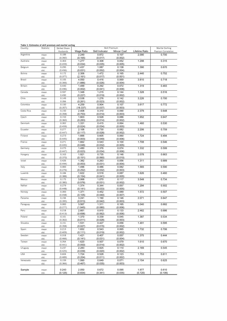
Table 1 reports the measures of the skill premium and sorting for each country.The first column reports the means and standard deviation of the fraction ofskilled husbands in our 36-45 years old husbands sample for each country. Thecolumn labelled “Skilled Share” gives the percent of the sample with more thanhigh-school education. The mean level of the share of skilled husbands acrosscountries in our sample is 24.3% with a standard deviation of around 12.5%. Thenext four columns show di erent measures of the skill premium. The averagelevels of both the wage ratio and of the lifetime income ratio is around 2 with astandard deviation close to 0.8 for the wage ratio and 0.7 for the lifetime incomeratio. The means and standard deviations for the skill indicator measure and theMincer coe cient are 0.67 (0.34) and 0.095 (0.035), respectively. The last columnreports the sample correlation measure of marital sorting. On average acrosscountries, the sample correlation between spouses’ years of schooling is about0.61 with a standard deviation of 0.11. The countries with the lowest skill premiaare Australia and Denmark (wage ratio) and Poland (Mincer coe cient), whileColombia and Brazil (wage ratio) and Bolivia and Paraguay (Mincer coe cient)have the highest. The correlation of the years of schooling across spouses is lowestfor Australia, and highest for Colombia and Ecuador. As shown in Table 2, ourfour measures of the skill premium are highly correlated with each other (over0.8). All of the correlations are significant at the 1% level.
3.3. Results
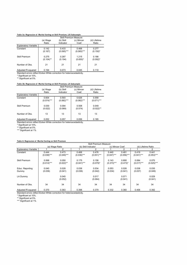
This section reports the main results of our empirical analysis. Note first fromTable 2 that marital sorting is positively and significantly correlated with allour measures of the skill premium (around 0.6 in each case). Table 3 showsthe results from a regression of marital sorting on the skill premium, using ourfour di erent measures of the skill premium. The standard errors of the OLSregression are based on the Eicker-White robust covariance matrix in order tocorrect for heteroskedasticity. For each measure of the skill premium we haveincluded two specifications of the regression. Specification 1 in Table 3 simplyregresses sorting on the skill premium. We find that this relationship is positiveand significant at the 1% level for all our measures. Thus, our first empirical testagrees with the basic prediction of our theory of a positive correlation betweenthese two variables.Figures 3 and 4 show the data used in the regressions of Tables 3 for the wage
ratio and the Mincer coe cient measures of the skill premium (the skill indica-
24
tor and lifetime income ratio estimates look similar to these). As is clear fromthese figures, Latin American countries tend to have a greater degree of inequalitythan the rest of our sample. One possible interpretation of this finding is thatthe Latin American countries are in a steady state with high inequality and highsorting whereas the rest of our sample (predominantly European countries) are ina low inequality-low sorting steady state with the variation within these subsam-ples being explained by country-specific factors (e.g., labor-market institutions,education and tax policy, credit markets, etc.). To make sure that our results arenot driven by some factor other than sorting that is common to Latin Americancountries, specification 2 in Table 3 introduces a Latin American dummy variableinto the regressions. As can be seen, sorting is still significant, although now atthe 5% level.31
We also examined the correlation between marital sorting and the skill pre-mium within our Latin American (LA) and LIS subsamples. For the LIS subsam-ple, the results, as shown in Table 3a, are similar to those of Table 3. .For the LAsubsample, the relation although positive is usually not significant, which is notsurprising, given the small size of the subsample.We next examine whether the way variables are reported and how we assign
years of education might a ect our results. As we have noted previously, some LIScountries report years of education whereas some report only the highest formallevel attained, such as high-school diploma or undergraduate degree. As a result,for some countries the years of education or skilled category includes only thosewho have completed college or the appropriate degree and excludes those who havenot obtained the pertinent degree but may have progressed beyond high school. Inorder to check whether this feature of our data a ects our results, the regressionsin Table 4 include a dummy variable that takes the value of 1 for countries whichreport the finer classifications of education and zero otherwise. As Table 4 shows,inclusion of this variable does not a ect the sign of the sorting e ect (althoughthe significance drops). Furthermore, when the Latin American dummy variableis included, the education-reporting variable has no additional explanatory powerand the adjusted R-squared is slightly lower. Again, this is to be expected, asall Latin American countries report years of schooling, which makes the dummyvariables very highly correlated.Another potential concern is that although we have examined each country’s
education system to understand how it progresses, the actual number of years of
31We also checked for outliers that shifted the estimated coe cient on the skill premium bymore than one standard deviation; there were no outliers.
25
schooling that we assign to each attainment level may a ect our measure of maritalsorting. A possible check is to use the Spearman rank correlation between yearsof schooling of husbands and wives as an alternative measure of sorting. Therank correlation measure of sorting and sample correlation measure are highlycorrelated (0.98). Our results also go through with this measure, although whena Latin American dummy is introduced the coe cient becomes insignificant fortwo of our skill premium measures.As noted previously, some countries report earnings net of taxes and some
report gross earnings. Since, due to progressive taxation, gross earnings will ingeneral tend to be more unequal than the net ones, this can create di erences inthe measured skill premium and a ect our results. In order to control for the wayincome is reported, we introduce a dummy variable that takes a value of 1 if thea country reports net earnings and 0 otherwise. The results are reported in Table5. The e ect of this dummy variable is positive but not significant. As in Table3, all four measures of the skill premium still have a positive and significant e ecton sorting, indicating that our results were not driven by this particular featureof the data.
3.4. Other Issues
In our model the e ect of the skill premium on marital sorting is independent ofthe fraction of the population that is skilled (other than endogenously through thee ect of on the skill premium). This, however, would not be the case in a largeset of models in which individuals meet others at random.32 Thus, one mightexpect that a population with a higher , for a given skill premium, would havea greater degree of sorting as skilled individuals (or more educated individuals)know that they have a higher chance of meeting another skilled individual in thefuture. This would tend to make them less willing to match with an unskilledindividual. In Table 6 we examine this issue by controlling for the fraction ofskilled individuals in each country in our OLS regression. In all specifications thee ect of the skill premium on sorting is positive and significant, at the 1% levelwithout a Latin American dummy, and at 5 or 10% with it.33 Furthermore, the
32Even if individuals would for sure be given the opportunity to meet only others from theirown skill group in the last period, a model with more than two rounds of matching and dis-counting would also produce dependence of the cuto quality level for a mixed match on thefraction of skilled people.33We also controlled for a quadratic relationship in with similar results.
26
e ect of the population skill level is negative, an issue that we investigate in moredetail below.Although our results in Table 3 indicate a positive and significant correlation
between marital sorting and the skill premium, a natural concern is that thecorrelation is driven by some third factor that is positively correlated with ourvariables. We next turn to an examination of various possible candidate variablesthat could be driving our results.A possible (presumably exogenous) variable that could a ect both sorting and
the skill premium, it could be argued, is the country’s degree of ethnic fraction-alization. Note though that the argument must be stronger than the fact thatindividuals tend to marry others from the same ethnic origin and that for variouspolitical economy arguments (e.g. Alesina, Beqir, and Easterly (1999)), countrieswith greater degrees of ethnic fractionalization have greater degrees of inequality.It must also argue that ethnic groups di er in their human capital so that sortingalong ethnic lines translates into sorting along the education dimension. Whythis should be so is not clear. One possibility, however, might be the reluctance ofan ethnically dominant group to invest in public services (such as schooling) forother ethnic groups (e.g. Easterly (2001)). We examine this issue by introducinga variable that captures the degree of ethno-linguistic fractionalization within thecountry. This variable, which take values between 0 and 100 with higher val-ues indicating more fractionalization, is taken from World Bank Growth Network(WBGN) data set.34 For our set of countries (excluding the Czech Republic,Hungary, Poland and Slovakia for which data was not available) the degree ofethno-linguistic fractionalization ranges from a minimum of 3 (Germany) to amaximum of 75 (Canada) with a mean value of 26.3 and a standard deviation of20.8.Next we consider the possibility that a country’s degree of urbanization may be
driving our results. Cities, it can be argued, are places where one may expect tohave greater mixing among di erent types than in the countryside where the skillacquisition may tend to be more uniform. Thus, if countries whose populationis more concentrated in cities tend to have lower skill premia (perhaps due tobetter borrowing opportunities in cities), this might be responsible for our findingof a positive correlation between sorting and the skill premium. To examine thishypothesis we introduce an urbanization variable which we take from the WBGNdata set as well. This is the fraction of a country’s population living in urbanareas in 1990 as reported to United Nations by each country. In our sample,
34This variable is available at http://www.worldbankorg/research/growth/GDNdata.htm
27
the lowest value for urbanization is 47.1 (Costa Rica) and the highest value is96.5 (Belgium). Overall, the mean value for urbanization is 73.3, with a standarddeviation of 13.2.Another possible concern is that our results are driven by the fraction of labor
force that is female. The argument here would have to be something alongthe lines that in countries in which a greater fraction of woman work, the skillpremium is lower (why women’s labor force participation should have this e ectis rather unclear), and furthermore there is less sorting as men and women fromdiverse educational backgrounds have greater opportunities to interact (i.e., theworkplace) than if women only went to school and then stayed out of the laborforce. This would then explain the positive correlation between the skill premiumand sorting. We examine this possibility by including a variable that measuresthe fraction of the labor force that is female. We take the 1990 values of thismeasure from World Bank (2001). In our sample (Luxemburg and Taiwan areexcluded since the data was not available), the lowest value for the fraction oflabor force that is female was 27.7 (Ecuador) and the highest was 48 (Finlandand Sweden) with a mean of 39.9 and a standard deviation of 6.2.A last concern is that all our results are driven by the level of GDP per capita.
Although GDP per capita is an endogenous variable in our model and hencelooking at its exogenous e ects is problematic (as we are unable to think of avalid instrument that survives the inclusion of a Latin American dummy), wenonetheless add it as a control (possibly reflecting aspects of income level that arenot captured in the model). The argument here would be that countries withlow income are more unequal (again, why this follows is not very clear—perhaps apolitical instability argument related to per capita GDP) and that when income islow, not marrying “down” matters more than when it is high.35 Thus, countrieswith low levels of GDP should also see higher levels of sorting. To evaluate thisargument we incorporate a measure of real per capita GDP (its 1997 value from theWBGN) into our regression analysis. The poorest country in our sample has a realGDP per capita of $1896 (Bolivia) and the richest one has $21974 (Luxembourg),while the average value for the whole sample is $9897, with a standard deviationof $5941.36
Table 7 reports the results of introducing each of these variables separatelyin a regression of marital sorting on the skill premium (using the wage ratio as
35This argument more generally depends on the the sign of the third derivative of the utilityfunction.36The data for Germany is from 1992.
28
the measure of the skill premium) as well as introducing them all jointly. As onemight expect from our argument above, ethnic fractionalization has a positiveand significant e ect on marital sorting. The e ect of urbanization on sortingis negative but not significant, whereas the faction of labor force that is femalehas a negative and significant e ect on marital sorting. In each specification(both with and without the additional control for Latin American) the coe cienton the skill premium remains positive and significant, although in the cases ofurbanization and GDP per capita, the significance drops to the 10% level whena Latin American dummy is included. In the regression with all the controlvariables, the positive e ect of the skill premium is significant at the 5% level.The results from these regressions indicate that the positive correlation be-
tween marital sorting and the skill premium is not an artifact either of the waysin which the data is reported nor of some obvious third factor. The positive corre-lation, nonetheless, does not allow us to determine whether the e ect of the skillpremium on sorting is truly positive or whether instead this relationship is drivenby the potentially positive e ect of sorting on the skill premium. We next turnto the question of causality.In our model both the skill premium and marital sorting are endogenously
determined variables. The timing of decisions though is that individuals firstsort given the expected skill premium. The e ect of current sorting, therefore,is only on future inequality rather than on the current skill premia since howindividuals sort a ects the proportion of individuals who will be able to becomeskilled the following generation. Consequently, the skill premium faced by our35-45 year olds is not simultaneously determined with their sorting patterns. Itcould be argued, however, that technology shocks that a ect the skill premiumtend to be serially correlated. If technology shocks are neutral and the productionfunction is constant returns to scale, however, then a measure such as the wageratio will not be a ected by these shocks. On the other hand, if shocks arenot neutral then this concern is valid since there will be a bias in the coe cientestimate resulting from the correlation of the explanatory variable with the errorterm. To correct for this endogeneity bias, we would like to find a variable thatis highly correlated with the explanatory variable but not with the error term inthe regression equation.Ex ante, an excellent candidate as an instrument for the skill premium would
appear to be the amount of capital per worker, since presumably it would bepositively correlated with the skill premium (if we think that capital and skilledlabor are more complementary than capital and unskilled labor), and there is no
29
reason to believe that it would have an independent e ect on the degree of sorting.The problem, however, with this instrument is that it does not capture enoughvariation across countries beyond those between countries from Latin Americanand the LIS sample.As an alternative, we also explored using a variable that measured the strength
of labor unions is a potential instrument since it could a ect the skill premium butshould not have any direct e ect on marital sorting. As an instrument, however,it has the same problem as capital per worker. While the strength of labor unionsis negatively and significantly correlated with the skill premium, the significantrelation disappears once we control for being a LA country.37
Another possible instrument for the skill premium is the average years ofschooling in a country, since one might expect countries with a higher skilledshare of the population (and hence a lower skill premium according to our model)to have higher average years of schooling. Furthermore, this is a variable thatevolves slowly over time. According to our model, this variable would not havean e ect on sorting other than through its e ect on the skill premium. As wediscussed above, however, one could easily modify the search portion of our sort-ing model such that the skilled share of the population (and hence presumablyaverage years of schooling) has an independent e ect on marital sorting. As aresult, when we use the years of schooling as an instrument, we also include thefraction of skilled population as an additional control.Table 8 shows our two-stage least squares (2SLS) estimates of the correlation
between our di erent measures of the skill premium and marital sorting. We usethe measures of average years of schooling for the population aged 25 and abovegiven in Barro and Lee (2000). Overall, in the first stage regressions without anadditional Latin American dummy, both years of schooling and the skilled share ofthe population are negatively and significantly correlated with di erent measuresof the skill premium (except for with the Mincer coe cient, for which the skilledshare has no significant e ect). Once we add an additional LA dummy into thefirst stage regressions, the e ect of the skilled share diminishes, possibly reflectingthe fact that LA countries in general have a lower skilled share.In the second stage regressions, the e ect of the skill premium on marital
sorting is positive and highly significant. Furthermore, as expected, the e ectof the skilled share of the population on marital sorting is positive. Indeed, the
37We used total trade union membership as a percentage of the total labor force and workerscovered by collective bargaining as a percentage of total salaried workers as two di erentmeasures of the strength of unions (data from Rama and Arcetona (2000))
30
estimates of the e ect of the skill premium on marital sorting are significantlylarger than the ones we obtained from OLS. The estimate of 0.15 on the wageratio, for example, implies that going from a more equal country like Sweden toan unequal one like Chile results in an increase in the correlation coe cient forspouses education of about 0.31 points. The fact that the e ect of being a LatinAmerican country on marital sorting is negative indicates that once we account forthe skill premium, Latin American countries tend to have lower marital sorting, aresult that is rather hard to interpret in light of our previous finding of a positivecoe cient on this dummy variable. Finally, the finding of larger estimates on ourvarious measures of the skill premium in the IV regressions above might suggestthat downward bias due to measurement error in the skill premium might be largerthan the potential reverse causality problem.A potential problem with our instrument, however, is that one could imagine
that years of schooling might have an independent (presumably negative) e ecton sorting by allowing people to mix for a greater amount of time before finallyseparating across skill lines. This consideration suggests that our IV resultsshould be approached with some caution.38
3.5. Per Capita Income, Skilled Population and Sorting
We now turn to an examination of another prediction of our model: the exis-tence of a negative relation between marital sorting and per capita income acrosscountries. Note that our model implies that across steady states, economies (withthe same technology) are characterized by a positive relationship between sort-ing and the skill premium and a negative relationship of these with the fractionof skilled individuals. Consequently, ceteris paribus, we expect economies withsimilar technologies but with greater sorting to have lower per capita income astheir level of human capital will be further below the e cient level. We turn toan examination of this relationship in the data.Figure 6 shows the relation between marital sorting and per capita income
where per capita income is real GDP per capita in 1997. Note that althoughper capita output is an endogenous variable in our model, the timing is suchthat sorting will a ect future output (rather than being a ected by it). Table9 shows the regression results for a specification in which the dependent variableis our measure of per capita income and the explanatory variable is the samplecorrelation measure of marital sorting with and without a Latin American dummy.
38We thank Torsten Persson for bringing this point to our attention.
31
The relation is significant and negative for both specifications as predicted by ourmodel.
4. Conclusion
This paper has examined the relationship between marital or household sortingand income inequality. Using a general equilibrium model in which individualsmake decisions over whether to become skilled or unskilled, about with whom tomatch, how much to consume, and the number of children to have, we find thatthere is a positive relationship between sorting and inequality (between skilled andunskilled workers). In particular, whether at a point in time, or across steadystates, economies with greater skill premia should also display a greater degree ofsorting. Our model also predicts that economies with greater skill premia shouldhave greater fertility di erentials, and (given identical technologies) economieswith greater sorting should have lower per capita income and smaller fractions ofskilled workers.Our empirical work is based on household surveys for 34 countries. From these
surveys we create our main sample for each country, a measure of marital sorting,and various measures of the skill premium. Our regression analysis supports ourcentral prediction of a positive relationship between sorting and inequality acrosscountries even after controlling for other possible sources of this correlation. Wealso find evidence in favor of a negative relationship between sorting and per capitaincome as predicted by our model as well.It should be noted that our story of greater pickiness with respect to household
partners in the face of an increased skill premium is of course not the only onecompatible with a positive correlation between these two variables. An alterna-tive story, with similar mechanics, would be of greater sorting into communities orschools in response to greater inequality (say, in response to fear of more crime).This could then lead to fewer opportunities to interact between individuals ofdi erent skill groups and consequently to a greater correlation of spouses in ed-ucation. We do not see this mechanism as being very di erent. Once again,private decisions that are sensitive to the degree of inequality (e.g., where to live,where to go to school) would feed through to marital decisions, which would thenhave important social consequences as a result of borrowing constraints.There are many directions in which this work could be extended. We have ab-
stracted from several issues, each of which are of interest in their own right. First,we have ignored di erences between men and women. An alternative formulation
32
of our model would be to have parents care about the quality and quantity of theirchildren and for parental time and education to be a factor in producing quality(perhaps by lowering the cost of the children becoming skilled). Thus, a parentwho stayed at home and took care of the children would contribute to householdutility by increasing the quality of their o spring. If, because of childbearingcosts this were predominantly the woman, men would still wish to match withmore educated women either because of their earning potential (as in the model)or because of the increased quality of the children. Thus, a major topic we wishto investigate (theoretically and empirically) is the relationship among sorting,female wage inequality and male wage inequality.39 This would also tie in withanother set of issues that we have chosen to ignore—that of household bargaining,the option to remain single and the possibility of divorce. Another avenue to ex-plore is the importance of bequests relative to education in the intergenerationaltransmission of inequality. Lastly, it would be interesting to examine the role ofpublic policy (education subsidies and welfare policy) in interacting with sortingand inequality. We plan to study several of these issues in future work.
39See Galor and Weil (1996) for a model in which exogenous di erences between women andmen leads to a large gap between the wages of these at low levels of capital, which is then reducedas capital accumulates. They use this model to help explain the demographic transition.
33
References
[1] Aiyagari, S. Rao, J. Greenwood, and N. Guner. “On the State of the Union.”Journal of Political Economy, 108 (2000), 213-244.
[2] Alesina, Alberto, R. Baqir, and W. Easterly, “Public Goods and Ethnic Di-visions,” Quarterly Journal of Economics, CXIV (1999), 1243-1284.
[3] Barro, Robert J. and J. W. Lee, “International Data on Educational Attain-ments: Updates and Implications,” mimeo, (2000).
[4] Becker, Gary S. “A Theory of Marriage: Part I,” Journal of Political Econ-omy, 81 (1973): 813-846.
[5] Becker, Gary S. and N. Tomes, “An Equilibrium Theory of the Distributionof Income and Intergenerational Mobility,” Journal of Political Economy, 87(1979), 1153-1189.
[6] , “Human Capital and the Rise and Fall of Families,” Journal ofLabor Economics, 4 (1986), S1-S39.
[8] Bergstrom, Theodore C., “A Survey of Theories of The Family,” in Handbookof Population and Family Economics, Edited by M. R. Rosenzweig and O.Stark, Elsevier Science, 1997.
[9] Bils, Mark and P. J. Klenow, “Does Schooling Cause Growth?” AmericanEconomic Review, 90 (2000), 1160-1183.
[10] Boulier, Bryan L. and M. R. Rosenzweig, “Schooling, Search, and SpouseSelection: Testing Economic Theories of Marriage and Household Behavior,”Journal of Political Economy, 92 (1984), 712-732.
[11] Burdett, Kenneth and M. G. Coles, “Marriage and Class,” Quarterly Journalof Economics, 112, (1997), 141-168.
[12] , “Transplants and Implants: The Economics of Self-Improvement,” mimeo, (1999).
34
[13] Cole, Harold L., G. Mailath, and A. Postlewaite, “Social Norms, SavingsBehavior and Growth,” Journal of Political Economy, 100 (1992), 1092-1125.
[14] Dahan, Momi and D. Tsiddon, “Demographic Transition, Income Distribu-tion and Economic Growth,” Journal of Economic Growth, 3 (1998), 29-52.
[15] Dahan, Momi and A. Gaviria, “Sibling Correlations and IntergenerationalMobility in Latin America,” mimeo, (1999).
[16] Durlauf, S., “A Theory of Persistent Income Inequality,” Journal of EconomicGrowth, 1 (1995), 75-93.
[17] Easterly, William, “The Middle Class Consensus and Economic Develop-ment,” mimeo, 2001.
[18] Fernandez, Raquel, “Education, Segregation, and Marital Sorting: Theoryand an Application to the UK,” mimeo, (2001).
[19] Fernandez, Raquel and C. A. Pissarides, “Searching for a Partner,” mimeo,(2001).
[20] Fernandez, Raquel and R. Rogerson, “Public Education and Income Distri-bution: A Dynamic Quantitative Evaluation of Education Finance Reform,”American Economic Review, 88 (1998), 813-833.
[22] Galor, Oded and J. Zeira, “Income Distribution and Macroeconomics,” Re-view of Economic Studies, 60 (1993), 35-52.
[23] Galor, Oded and D. Weil, “The Gender Gap, Fertility and Growth,” Ameri-can Economic Review, 86 (1996), 374-387.
[24] Greenwood, Jeremy, N. Guner and J. Knowles, “More on Marriage, Fertilityand the Distribution of Income,” mimeo, (1999).
[25] Knowles, John, “Can Parental Decisions Explain U.S. Income Inequality?”PhD Dissertation, University of Rochester, (1999).
[26] Kremer, Michael, “How Much does Sorting Increase Inequality,” QuarterlyJournal of Economics, 112 (1997), 115-139.
35
[27] Kremer, Michael and D. Chen, “Income Distribution Dynamics with En-dogenous Fertility,” American Economic Review Papers and Proceedings, 89(1999), 155-160.
[28] Laitner, John, “Household Bequests, Perfect Expectations, and the NationalDistribution of Wealth,” Econometrica, 47 (5), (1979), 1175-1194.
[29] Lam, David, “Marriage Markets and Assortative Mating with HouseholdPublic Goods: Theoretical Results and Empirical Implications,” Journal ofHuman Resources, 23 (1988), 462-487.
[30] Ljungqvist, Lars, “Economic Development: The Case of a Missing Marketfor Human Capital,” Journal of Development Economics, 40 (1993), 219-239.
[31] Loury, Glenn C. “Intergenerational Transfers and the Distribution of Earn-ings.” Econometrica, 49 (1981), 843-867.
[32] Mare, Robert D. “Five Decades of Educational Assortative Mating,” Amer-ican Journal of Sociology, 56, (1991), 15-32.
[33] Owen, Ann and D. Weil, “Intergenerational Earnings Mobility, Inequalityand Growth,” Journal of Monetary Economics, 41 (1998), 71-104.
[34] Perotti, Roberto, “Growth, Income Distribution, and Democracy: What theData Say,” Journal of Economic Growth, 1 (1996), 149-187.
[35] Pissarides, Chris, “From School to University: The Demand for Post-Compulsory Education in Britain,” Economic Journal, 92 (1982), 654-667.
[36] Rama, Martin and R. Artecona. “A Database of Labor Market IndicatorsAcross Countries,” The World Bank, mimeo (2000).
[37] Regalia, Ferdinando and J. V. Rios-Rull. “What Accounts for the Increasein Single Households and the Stability in Fertility?” mimeo (1999).
[38] Smits, Jeroen, W. Ultee, and J. Lammers, “Educational Homogamy in 65Countries: An Explanation of Di erences in Openness Using Country-LevelExplanatory Variables,” American Sociological Review, 63 (1998), 264-285.
36
[39] Weiss, Yoram. “The Formation and Dissolution of Families: Why Marry?Who Marries Whom? and What Happens upon Divorce?” in Handbookof Population and Family Economics, Edited by M. R. Rosenzweig and O.Stark, Elsevier Science, 1997.
[40] World Bank, World Development Indicators, 2001.
5. Appendix A
We will now show that all terms in the first curly bracket of equation (2.18) Beforedoing this, as we have already argued, q is strictly negative, since
q=
f 00
f 0(f 0(1 k) + f)| {z } ( ews wu)| {z }+
+ f 0(1 + k)(wu + ews )| {z }+
1
(1 )2< 0,(5.1)
where f 0(f 0(1 k) + f) = ews( ews + wu) > 0. Hence, all we want to determine isthe sign of the following expression
, this expression is increasing in wu, and we can evaluate at the limit
where wu = 2,
Aews¯¯wu= 2
= (1 + 2kQ + k2)( ews 2
4)
+(2k +Q k2 +Q )( ews + 2
4) 2 (k + k2Q ) ews.
38
Again, this expression is also increasing in ews (note that Q 1), therefore we canevaluate it at ews = 2
,
Aews¯¯ews= 2
,wu= 2
= (1+ 2kQ + k2)2
4+3 2
4(2k+Q k2+Q ) (k+ k2Q ) 2 > 0.
Thus A is increasing in ews and wu. To show that A is positive, we simply evaluateit at ews = wu = 2
:
A|ews= 2,wu= 2
= 0 + (2k +Q k2 +Q )3
4(k +Q )
3
4(k + k2Q )
3
4= 0
Hence, in Equation (2.18) all terms are negative except those withk.
6. Appendix B
The years of households surveys used in our empirical study are given in Ta-ble B1. All surveys are nationally representative samples, except for Argentinaand Uruguay for which we have only urban samples (70% of the population forArgentina and 90% for Uruguay). Table B1 also gives details of the income mea-sures available in each survey. The income in the Latin American countries is grossmonthly labor income from all sources. This definition varies across countries, butgenerally includes wages, income from self-employment, proprietor’s income, fromboth primary and secondary labor activities. Some LIS countries report grossannual earnings and income and some report these net of taxes.40 We use grosslabor earnings for LIS countries whenever it is available. The gross earnings mea-sure for LIS countries include all forms of cash wage and salary income, includingemployer bonuses, 13th month bonus, etc., (gross of employee social insurance con-tributions/taxes but net of employer social insurance contributions/taxes). Whilemost countries report gross earnings, the following countries report only the netearnings: Belgium, France, Hungary, Italy, Luxemburg, Poland, and Spain. Sincetaxation tends to be progressive in the countries we are comparing, inequality ofincome is likely to be higher than reported in those countries for which pre-taxincome is not reported. We do not adjust income measures in LIS or IDB for
40Some LIS countries are excluded because they do not report all of the variables requiredfor the analysis. Ireland and Austria do not report individual labor income. Ireland also doesnot report the education of the spouse in the household sample. Education variables are notavailable for Switzerland.
39
hours worked or weeks worked in order to arrive at a measure of total income,including leisure. This is because few countries collect hours or weeks series, andsome of those that do collect them, such as Slovakia or Spain, use discrete codesrather then report actual levels.Education in the Latin American data is reported as total years of schooling.
For the LIS countries the education units are quite idiosyncratic. We attempt tostandardize the LIS education variable by converting the reported units to years ofeducation. We define as skilled all agents who went beyond high school education.For some of the Latin-American data, this coincides with indicator variables forhigher education, as a few of these countries report attainment in addition to yearsof education. For the other Latin-America countries, this indicator is constructedusing the standard age-grade progression for that country. Thus, skilled workersin Costa Rica, for example, are those with more than 11 years of education, whilein Mexico, they are those with more than 12 years. For Britain we would havepreferred to define as skilled any individual with at least 2A levels passes (asin Fernandez (2001) or Pissarides (1982)), but as the data did not permit usto distinguish among individuals with di erent number of A levels, we insteadcategorized them all as unskilled. Our results are robust to categorizing them allas skilled instead. Table B2 reports our mapping of education measures into yearsof schooling and into an indicator for high school completions. For most countries,we were able to compare the percentage of adults with education beyond the high-school level to published sources, and to reconcile our statistics with the previouslypublished numbers.
40
δ = Ψ(λt+1; λt)
δ* (λt+1) = Vs(λt+1)-Vu(λt+1)
λt+1
δ
δ**
λ**
Figure 1
0.0 0.1 0.2 0.3 0.4 0.5 0.6 0.7 0.8 0.9
lambda
0.0
0.1
0.2
0.3
0.4
0.5
0.6
0.7
0.8
0.9
lam
bd
a-p
rim
e
45-degree
A
B
Figure 2
0.3 0.4 0.5 0.6 0.7 0.8
Sample Correlation Measure
1
2
3
4
5
Wa
ge
Ra
tio
ARGARG
AUSAUS
BELBEL
BOLBOL
BRABRA
BRIBRI
CANCAN
CHICHI
COLCOL
COSCOS
CZECZE
DENDEN
ECUECU
FINFIN FRAFRA
GERGER
HUNHUN
ISRISRITAITA
LUXLUX
MEXMEX
NETNETNORNOR
PANPAN
PARPAR
PERPER
POLPOL
SLOSLOSPASPA
SWESWE
TAITAI
URUURU
USAUSA
VENVEN
Figure 3 --- Inequality and Sorting
0.3 0.4 0.5 0.6 0.7 0.8
Sample Correlation Measure
0.04
0.06
0.08
0.10
0.12
0.14
0.16
0.18
Min
cer
Co
ef.
ARGARG
AUSAUS
BELBEL
BOLBOL
BRABRA
BRIBRI
CANCAN
CHICHI COLCOL
COSCOS
CZECZE
DENDEN
ECUECU
FINFIN
FRAFRA
GERGER
HUNHUN
ISRISR
ITAITA
LUXLUX
MEXMEX
NETNET
NORNOR
PANPAN
PARPAR
PERPER
POLPOL
SLOSLO
SPASPA
SWESWE
TAITAI
URUURU
USAUSA
VENVEN
Figure 4 --- Inequality and Sorting
0.3 0.4 0.5 0.6 0.7 0.8
Sample Correlation Measure
0
2000
4000
6000
8000
10000
12000
14000
16000
18000
20000
22000
GD
P p
er C
apita
Figure 5 --- GDP per capita and Sorting
ARGARG
AUSAUS
BELBEL
BOLBOL
BRABRA
BRIBRI
CANCAN
CHICHI
COLCOLCOSCOSCZECZE
DENDEN
ECUECU
FINFINFRAFRA GERGER
HUNHUN
ISRISR
ITAITA
LUXLUX
MEXMEX
NETNET
NORNOR
PANPAN
PARPARPERPER
POLPOLSLOSLO
SPASPA
SWESWE
TAITAI
URUURU
USAUSA
VENVEN
Table 1: Estimates of skill premium and marital sortingCountry Statistic Skilled Share Marital Sorting
Husbands Wage Ratio Skill Indicator Mincer Coef. Lifetime Ratio Pearson Correlation
Argentina mean 0.189 2.249 0.872 0.107 2.090 0.700std. (0.392) (0.165) (0.017) (0.002) . .
Australia mean 0.303 1.277 0.308 0.052 1.298 0.315std. (0.459) (0.034) (0.035) (0.005) . .
Adjusted R-squared 0.458 0.612Standard errors reflect Eicker-White correction for heteroscedasticity.* Significant at 10%.** Significant at 5%.*** Significant at 1%
TABLE B1: Survey InformationCountry Number of
Households
Australia 1994 Australian Bureau of Statistics
Belgium 1992 Centre for Social Policy 3821
INSEE
Division Conditions de vie des Ménages
Statistical Office of the Slovak Republic
Division of SocialStatistics and Demography
Statistics Sweden
Program for Income and Wealth
Academia Sinica
Bureau of Labor Statistics
16323 National
Australian Income and Housing Survey
Panel Survey of the Centre for Social Policy
Endre Sik / Istvan Toth
Israeli Central Bureau of Statistics
Ufficio Informazioni Statistiche
Centre d'Etudes de Populations, de Pauvreté et
de Politiques Socio-Economiques
Centraal Bureau voor de Statistiek
Statistics Norway
Venezuela 1996 Encuesta de Hogares por Mustreo Oficina Central de Estadistica e Informatica
Urban
1994 March Current Population Survey 66014 National
1996 Encuesta Continua de Hogares instituto nacional de Estadistica 19322
National
National
National
1995 Survey of Personal Income Distribution 14706 National
1995 Inkomstfördelningsundersokningen 16260
1990 Expenditure and Income Survey 11294 NationalInstituto Nacional de Estadistica
with Leaving ExamSpain 12 Secondary Education/Basic Tech. Edu.Sweden 12 Secondary SchoolTaiwan 10,12 Senior High/Vocational GraduateUruguay 11 N/AUSA 12 High School DiplomaVenezuela 11 N/A* Finland, Israel and Norway report years of education