Essays on Sovereign Default A THESIS SUBMITTED TO THE FACULTY OF THE GRADUATE SCHOOL OF THE UNIVERSITY OF MINNESOTA BY Laura Sunder-Plassmann IN PARTIAL FULFILLMENT OF THE REQUIREMENTS FOR THE DEGREE OF Doctor of Philosophy Timothy J. Kehoe May, 2014
Transcript
Essays on Sovereign Default
A THESIS
SUBMITTED TO THE FACULTY OF THE GRADUATE SCHOOL
OF THE UNIVERSITY OF MINNESOTA
BY
Laura Sunder-Plassmann
IN PARTIAL FULFILLMENT OF THE REQUIREMENTS
FOR THE DEGREE OF
Doctor of Philosophy
Timothy J. Kehoe
May, 2014
c� Laura Sunder-Plassmann 2014
ALL RIGHTS RESERVED
Acknowledgements
I am indebted to my adviser and the members of my committee without whom this thesis
would not exist: I would like to thank Tim Kehoe and Fabrizio Perri for all their support
and guidance throughout my time at Minnesota; I am very grateful to Cristina Arellano
for her advice, encouragement, and for her door being always open for me; and I would like
to thank Terry Roe for serving on my committee and for his feedback on my work. Finally,
thanks to my fellow grad students for their suggestions, comments, help and friendship.
i
Dedication
To my parents, Ulrich and Eva.
ii
Abstract
This thesis consists of three separate chapters. In the first chapter, I review the literature
on sovereign debt crises. In the second chapter, I analyze the role nominal debt plays
in sovereign debt crises, and in particular default and inflation policies. Using bond-level
data on government borrowing, I document that nominal obligations are a large fraction of
government debt in emerging market countries. I then show that default and inflation rates
vary systematically with debt denomination: high nominal debt shares are associated with
low inflation and default rates in these countries. I build a monetary model of sovereign debt
with lack of commitment, in which di↵erences in debt denomination generate this pattern,
and the government inflates more when debt is real. Issuing real instead of nominal debt
has two e↵ects in the model. On the one hand, real debt reduces the incentive to create
costly inflation because the value of the debt is fixed in real terms. It thus helps mitigate
the commitment problem. On the other hand, because the commitment problem is less
severe, real debt facilitates more debt accumulation over time, causing the government to
resort to the printing press after all to finance the debt burden. In a calibrated version
of the model this second e↵ect dominates: As in the data, inflation and default rates are
higher on average when debt is real instead of nominal. Default risk helps generate large
di↵erences in inflation and default rates across debt regimes as the government optimally
inflates in order to avoid default.
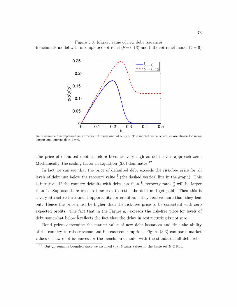
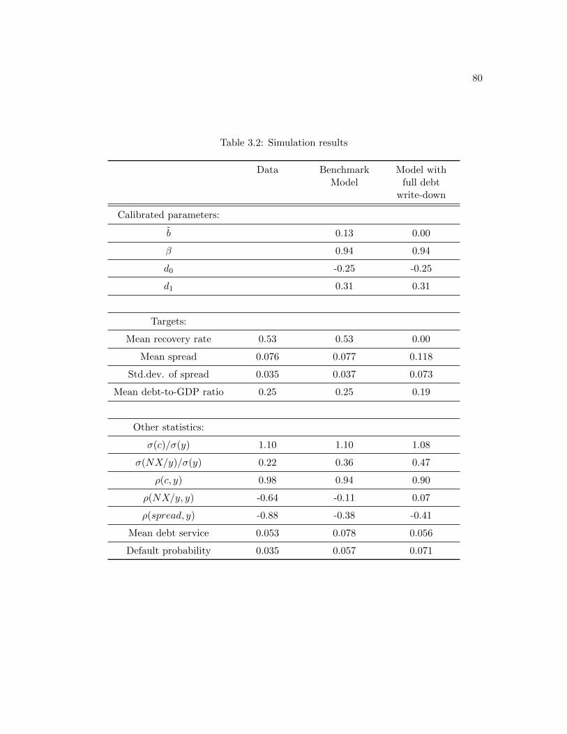
In the third chapter, I study incomplete debt relief in sovereign debt crises. I show that,
in the data, sovereign defaults typically do not result in a full debt write-down. On the
contrary, creditors recover on average more than half of their investment. I then build a
model of sovereign default and incomplete debt relief to study the causes and consequences
of incomplete debt relief. In the model, the degree of debt relief directly a↵ects default
incentives via bond prices. In particular, a high debt recovery rate - equivalently, little
debt relief - reduces recovery risk to investors and tends to o↵set the e↵ects of default
risk. In equilibrium, incomplete debt relief lowers spreads and increases debt-to-output
ratios and welfare. Default rates are non-monotonically related to debt relief and lowest
for intermediate, but relatively low degrees of debt relief. I use the model to analyze the
iii
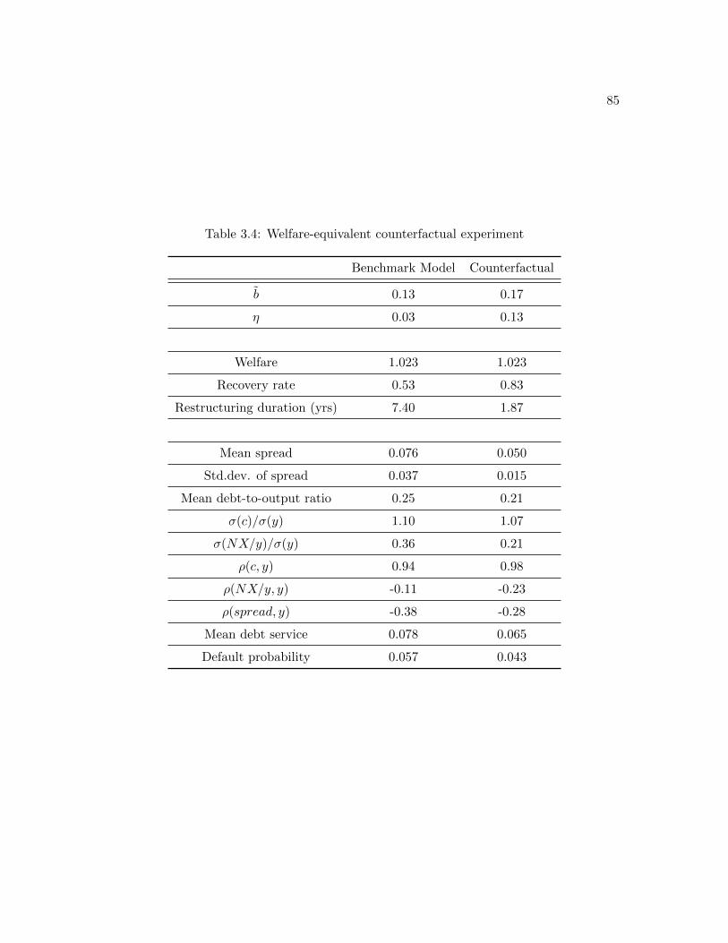
trade-o↵ between long renegotiations and low debt relief and show that the latter is a more
e↵ective tool for achieving low equilibrium default rates and high welfare. Finally, the
model predicts that countercyclical recovery rates are not welfare-improving.
3.6 The trade-o↵ between restructuring duration and debt relief . . . . . . . . 87
A.1 Aggregate bond debt in my sample of countries . . . . . . . . . . . . . . . . 110
A.2 Raw scatter plot of inflation against nominal debt share . . . . . . . . . . . 110
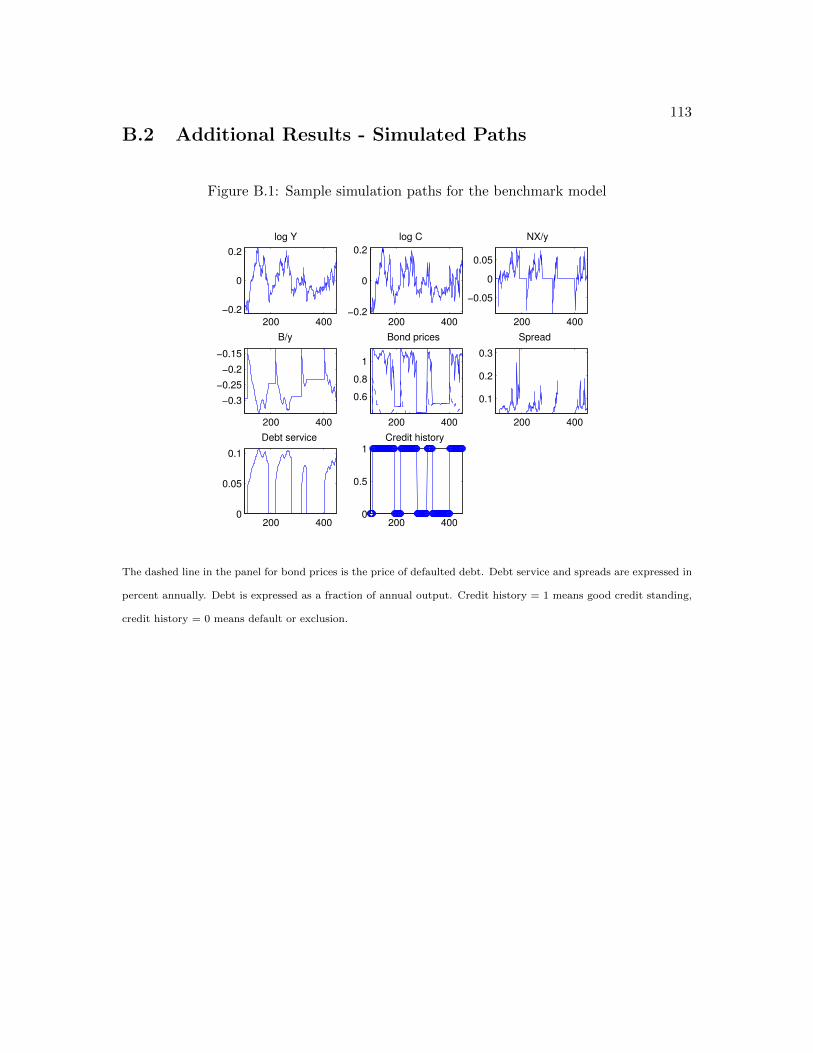
B.1 Sample simulation paths for the benchmark model . . . . . . . . . . . . . . 113
viii
Chapter 1
Critical Review
The key distinguishing feature of sovereign borrowing is the lack of incentives for the bor-
rowing country to repay its creditors. Sovereign borrowing unlike other types of borrowing
involves no recourse for lenders by the very nature of sovereignty. International lending
is typically unsecured, international courts do not have the legal authority to seize assets,
and there are no international bankruptcy laws. As a result, theoretical approaches to the
topic have in common a focus on modeling environments with limited commitment, and
dealing with the question of how debt is sustainable in equilibrium. Absent an enforcement
mechanism, the government cannot commit is tempted to default on any outstanding debt.
It is then not clear why creditors in turn would ever lend in the first place in such a set-
ting. The benchmark quantitative sovereign default theory that I focus on in this chapter
rationalizes borrowing as a consequence of impatience by the government and default as
an opportunity to create state contingency in otherwise incomplete markets. Default is an
infrequent event and equilibrium debt levels are positive in the theory because default is
costly in di↵erent ways.
While early theoretical studies were successful at accounting for some of the high level
empirical regularities - such as equilibrium default, countercyclical interest rates - they did
abstract from many other features of default and an active literature has developed that
is filling these gaps. Aspects that have received particular attention include theories of
the maturity structure of sovereign debt and its implications for default, debt renegotia-
tions and debt relief, the link between sovereign risk and other aspects of fiscal policy and
1
2
the real side of the economy, and the links of sovereign debt crises to other crises. These
theoretical advances have been accompanied by empirical studies documenting novel facts
about sovereign crises and calling attention to their heterogeneity and previously unexam-
ined details. This includes moving from treating default as a binary indicator to measuring
partial default, studying maturity and denomination of debt, determinants of haircuts and
other aspects of sovereign debt renegotiations, as well as the relation of sovereign borrowing
to the business cycle.
In the following, I will review this literature on sovereign debt and default, starting
with empirics before moving on to the theoretical literature and discussing how the two
match up.
1.1 Empirical Literature
In this section I will review aspects of empirical research on sovereign debt and default. I
will first discuss measurement and definitional issues before reviewing empirical regularities
that the literature has established. The two are closely linked and important progress has
been made in recent years by looking at sovereign debt markets and crises in a more
disaggregated manner and focusing on more careful measurement.
1.1.1 Concepts and Measurement
1.1.1.1 Types of Government Liabilities
What do we mean when we talk about sovereign debt? Most studies are concerned with
external debt. This can be taken to mean debt issued in foreign rather than domestic cur-
rency, debt held abroad rather than at home, or debt issued under a foreign jurisdiction.
In practice with debt being bonded and freely tradable, keeping track of the residence
or nationality of the holder of the debt is di�cult, so studies have more often used de-
nomination or jurisdiction when defining external sovereign debt. We can furthermore
distinguish between debt issued by the national government as opposed to local or regional
governments or net of cross-holdings by the central bank or other government branches.
Sovereign debt today most often comes in the form of bonds issued that can be traded
on secondary markets. Other forms of sovereign debt include bank loans and lending by
3
international institutions like the IMF - both of these are more di�cult to value at market
prices but studies like Tomz (2007) document bond finance outstripping bank loans for
the past two decades, and according to the WDI, while concessional debt is a substantial
fraction of external debt for some countries, it is below 3% of GDP every year since 1970
(GDP-weighted average across countries). Within the domain of bonded debt, there are
many di↵erent kinds of bonds that can be issued. Even though the majority of sovereign
bonds are plain vanilla type bonds - pay at maturity, simple deterministic coupon structure
- there are exceptions, for example inflation-indexed debt, hybrid bonds, callable bonds and
variable rate bonds.
The link between external debt and debt that is in foreign currency and held abroad is
becoming increasingly weak in the data. Traditionally when talking about external debt
studies tend to consider exclusively foreign currency denominated debt issued on foreign
markets, assumed to be held by foreign investors. There is evidence that these distinctions
are beginning to blur: Local currency debt is increasingly held by foreigners (Du and
Schreger (2013)) and foreign currency debt is issued at home (Chapter 2).
1.1.1.2 Valuation of Liabilities
How should government debt obligations be valued to construct a measure of a sovereign’s
indebtedness? Most sources, including for example the World Bank, use the face value
to arrive at a measure of the stock of sovereign debt - that is the undiscounted sum of
future principal payments. This has the advantage of being simple to compute but there
are drawbacks. For example, the measure does not take into account coupon payments,
which make up a substantial fraction of bond payments in emerging markets and Latin
America in particular - a bond with no coupon payments is treated as the same obligation
as a bond with the identical principal amount that in addition makes coupon payments
regularly before maturity. In addition, it does not discount payments to be made in the
future - the consol whose face value is due in an infinite number of period receives as much
weight when calculating the stock of debt as a payment that is due tomorrow.
Possible discounts for future payment streams are market rates, or alternatively fixed
interest rates that capture at least some of the opportunity cost of holding the given debt
instrument. In practice, bond markets except for large issuers are often too illiquid to
4
estimate yield curves and hence market rates, but certainly for developed countries and
large emerging market issuers these are readily available from public sources.
Examples where valuation questions are relevant include measuring the maturity and
currency composition of government debt. Both of these involve decisions on the best mea-
sure of debt to use - face value, market value, including or excluding coupons, converting
future payment streams from one currency to another. To take the example of the maturity
of debt, a common measure to use is Macaulay duration - a cash-flow weighted average of
the dates of future cash flows, where the discount used is typically a constant market yield,
so debt that is highly discounted will receive a lower weight. Absent new debt issuances,
during a crisis when yield curves are likely to be flatter than during normal times, short
debt would be given less weight on account of lower market values in calculating duration.
Similarly, for nominal debt or debt denominated in other currencies, inflation expectations
and expected exchange rate movements a↵ect the valuation of the debt and should factor
into the valuation of the debt - but are hard to come by in many cases where financial mar-
kets are not liquid enough and forward exchange rates or measures of inflation expectations
not readily available.1
It is worth pointing out that which measure of indebtedness is the appropriate one
depends often on the context and if the goal is to match a model to the data consistency
in measurement across model and data are important.
1.1.1.3 Defining Default
What does it mean for a government to default on its debt? Defining what constitutes
default is not uncontroversial. One common measure is a binary indicator as in Beers and
Chambers (2006) by Standard and Poor’s, for example. The ratings agency lists default
episodes back to 1824. They define a default as “the failure to meet a principal or interest
payment on the due date (or within the specified grace period)”. A default is defined
as resolved when “no further near-term resolution of creditors’ claims is likely”. When
payments are rescheduled, they are deemed a default in case the rescheduling is at less
favorable terms to the creditors than the original arrangement. Both of these are di�cult
to quantify precisely, as we will see in more detail below - the likelihood of no further
1 See more in Arellano and Ramanarayanan (2012), and Chapter 2
5
resolutions, and measuring whether reschedulings are at less favorable terms. Moreover,
this binary definition of default lumps together potentially very di↵erent situations - for
example, Argentina suspending payments on over 75% of its outstanding external debt,
compared with a rescheduling by a few months of interest payments on just one oil warrant
as in Venezuela in 2005. Recently there have been studies that to use arrears as a less coarse
measure of credit history; examples include Benczur and Ilut (2011), Arellano et al. (2013)
and De Paoli et al. (2009).
1.1.2 Empirical Regularities
Having described the main definitional and conceptual issues surrounding sovereign debt
and default, I will now outline empirical regularities regarding sovereign debt and default
that have been documented in the literature.
1.1.2.1 Default Frequency
Defaults occur with regularity throughout history. Tomz andWright (2008) study sovereign
crises for 176 sovereign entities going back to 1820. The unconditional default probability
in this sample - number of country-year pairs in default relative to total number of country-
year pairs - was 1.7%. Conditioning on defaulters or restricting the sample to post-1980
raises this number to 3% and 3.8% respectively. Given the discussion of the previous section
on measurement and definition of default episodes, Tomz and Wright (2008)’s caution that
a more robust measure of default frequency should be used to calibrate models - they
suggest the fraction of time spent in default, which is 18% in their sample.2
An alternative is to abandon the simple binary default structure and focus on arrears
instead, as mentioned above (for example in Arellano et al. (2013)). These measures
typically identify similar episodes but tend to di↵er on precise start and end dates of
default episodes. They have the advantage of taking a more disaggregated look at what
payments a sovereign refuses to make, given the heterogeneity in debt instruments that
countries typically issue (nominal or real, long or short debt, held abroad or domestically,
to name but a few examples). On the other hand, legal provisions in bond contracts where
2 Other references include Reinhart and Rogo↵ (2009) and Sturzenegger and Zettelmeyer (2007).
6
default on one bond triggers default on all others are increasingly common, so it remains
to be seen if partial default becomes a less relevant concept over time.
1.1.2.2 Cyclicality of Sovereign Defaults
Whether defaults happen during deep recessions (rather than causing them - see the pre-
vious section) remains controversial in the empirical literature. Tomz and Wright (2007)
find that default does appear to be associated with weak outcomes on the real side of the
economy, but perhaps only modestly so. In a sample of 175 countries between 1820 and
2005, defaults occurred in periods where output was below its HP-trend only 60% of the
time. The average deviation of output from trend at the start of a default episode was
1.6%. Output tended to recover during default episodes rather than deteriorate further.
De Paoli et al. (2009) on the other hand, in 39 defaults from 1970 to 2000, find large
output losses on the order of 5% per year during defaults, including during the first year of a
default. Like Tomz and Wright (2007) they use HP-filtered data to construct counterfactual
potential output, but they also run regressions to control for several other factors, unlike
Tomz and Wright (2007) who focus on unconditional correlations. Defaults in De Paoli
et al. (2009) are defined as a threshold on arrears rather than a contractual contract breach
(which should reduce the number of defaults they find, and/or shorten the time of a default
episode). De Paoli et al. (2009) highlight that twin crises are associated with larger output
declines than idiosyncratic default episodes. They also find that output losses increase the
longer a country takes to restructure their debts and exit default.3
Yeyati and Panizza (2011) using quarterly data for 39 emerging market countries be-
tween 1970 and 2005 find large recessions (GDP 3.4% below trend) just prior to a default.
They argue that quarterly data is the more suitable frequency at which to analyze data
to pick up sharp drops in output surrounding default episodes and resolve some of the
identification problem - did a country default because output was low, or was output low
because the country defaulted? This is discussed further in section 1.1.2.5.
3 This latter regularity is also documented in Benjamin and Wright (2009).
7
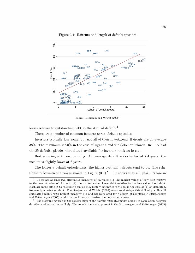
1.1.2.3 Haircuts and Debt Relief
Failure to pay on time - a default - does not mean that the payment or at least part of it will
never be made. In fact, despite lack of formal bankruptcy proceedings and enforcement
mechanisms, creditors to sovereigns recover on average more than half their investment
after a default. The flip side of this is that default does not actually reduce a borrower’s
indebtedness very much on average. Several recent papers have contributed to establishing
empirical facts on creditor losses or “haircuts” after sovereign defaults, including Cruces and
Trebesch (2011), Benjamin and Wright (2009) and Sturzenegger and Zettelmeyer (2005).
The main results from these empirical studies are that haircuts are high on average (37%
in the Cruces and Trebesch (2011) sample) and vary widely. Moreover, renegotiation length
is correlated with high haircuts, as is the cost of borrowing post-renegotiation. Cruces and
Trebesch (2011) also document that higher haircuts are associated with a lower likelihood
of regaining market access after a restructuring.4 It is to the best of my knowledge an
open an little researched question empirically whether debt relief is welfare improving (for
theoretical results on this see Chapter 3 and Section 1.2).5
Again, there are measurement issues involved: Benjamin and Wright (2009) base their
measure on WDI data which only considers face value reductions as haircuts, but not
maturity extensions like exchanging old instruments for new ones with later maturity dates.
In Sturzenegger and Zettelmeyer (2005)’s preferred measure they instead calculate haircuts
as the di↵erence in net present values between the original and the restructured debt. This
is harder to compute because it requires calculating prices of both the defaulted and newly
restructured debt at times of distress when markets are often illiquid and price quotes
not necessarily readily available. Cruces and Trebesch (2011) use the same measure of
haircuts but for a larger set of default episodes - the entire universe of sovereign debt
restructurings between 1970 and 2000, that is 182 restructurings by 68 separate countries.
Where comparisons between Benjamin and Wright (2009) and Cruces and Trebesch (2011)
are available, the measures are not close, so again, it is important to pick the appropriate
measure for the research purpose at hand and be sure empirical measures and model
4 Note that they define market access as borrowing after a successful restructuring of debt, not asmarket access during a default episode. See more on this in subsection 1.1.2.4.
5 There is a preliminary working paper by Wright et al. (2013) which finds welfare losses due to debtrelief.
8
counterparts are consistent (see Chapter 3).
1.1.2.4 Market Access
Several studies have examined whether and if so for how long defaulters are excluded from
borrowing again following a default - a quantity restriction rather than higher borrowing
costs. Some studies take “market access” to mean time until renegotiations are completed
successfully. Some take it to mean time until a defaulter can borrow again - which is a
di�cult question to answer for obvious endogeneity reasons.
Benjamin and Wright (2009) who belong to the first category of papers find that for
their sample of 90 defaults from 1989 to 2005 renegotiations took on average 8 years.
The Tomz and Wright (2007) sample leads to similar numbers. Gelos et al. (2011) define
market access as borrowing that leads to increased debt (in terms of face values) and find,
for defaults from 1980 to 2000, that it takes a much shorter amount of time after a default
until market access is restored - 4.7 years on average, and since 1990 even just 2.9 years.6
Cruces and Trebesch (2011) define market access as positive net transfers post-renegotiation
and find that it takes 5.1 years to regain market access.
Measurement di↵erences and questions of causality notwithstanding, regularities that
emerge from the literature are that there is at least some loss of market access following a
default, the length of exclusion is positively correlated with haircuts, and has fallen since
the 1980s.
1.1.2.5 Other Costs of Default
Aside from loss of capital market access and higher borrowing costs, many studies have
examined whether there are other costs of default.
Drops in GDP is one candidate that seems di�cult to pin down. Borensztein and
Panizza (2008) and Yeyati and Panizza (2011) for example have di�culty establishing
causality running from default to recessions and instead find evidence that recessions tend
to precede defaults and that output recovers in the course of default episodes. Clearly this
6 They exclude unresolved defaults like Argentina’s 2001 default. They measure market access as anincrease in debt in order to exclude cases where a country is unable to borrow but is able to rollover existingdebts.
9
needs to be taken with a grain of salt given the inherent endogeneity problem (see also
subsection 1.1.2.2).
Trade costs are another candidate where the evidence is inconclusive. Studies have
been able to identify falls in trade flows and trade credit. Rose (2005) finds in a sample
of 200 countries between 1948 and 1997 that Paris Club debt renegotiations are associated
with drops in bilateral trade of around 8% per year. Borensztein and Panizza (2010) using
industry level data show that especially exporters are a↵ected by these trade disruptions.
Borensztein and Panizza (2008) and Tomz and Wright (2013) argue that there is limited
evidence of direct trade embargoes following defaults, but Borensztein and Panizza (2008)
find evidence for trade credit disruptions arising from a spillover channel: Trade credit
becomes more expensive because private sector credit worthiness falls along with that of
the government. Arteta and Hale (2008) find similar evidence. There is no consensus
however on the exact channel through which default a↵ects either trade flows or trade
credit.
Cole and Kehoe (1998) in a theoretical contribution suggest reputational spillovers
from the sovereign’s willingness to repay to other areas of international relations. There is
relatively little empirical work on this but in one such study Tomz and Wright (2008) find
that sovereign default and other types of expropriation do not generally coincide, which
they say is at odds with the spillover hypothesis. Political costs of default more generally
are relatively under-researched empirically.7 Borensztein and Panizza (2008) note that
there is anecdotal evidence that defaults make political survival less likely, and that there
are reasons to suspect delay in initiating default on account of this. They argue that this
is one channel by which defaults could be more costly than otherwise the case.
1.1.2.6 Debt Maturity and Default
The maturity of debt varies significantly across countries and time, and how it changes with
risk of default depends on how it is measured. According to Tomz and Wright (2008) in a
sample of 137 low and middle income countries in the year 2000 the contractual maturity
(the payment date on any outstanding debt furthest into the future) ranged from 10 to
7 There is a large literature on costs of political instability, including debt accumulation and default,e.g. Easterly and Levine (1997).
10
40 years, whereas duration (the cash-flow weighted average of the dates of future cash
flows, discounted at a constant market yield) assuming a discount of 5% ranged from 3.4
to 14.2 years. Duration is shorter because of discounting, and because for emerging market
countries a relatively large part of obligations tends to come in the form of coupon payments
rather than the principal. Arellano and Ramanarayanan (2012) document that for four
major emerging market borrowers - Mexico, Russia, Brazil and Argentina - between 1996
and 2011, average duration for each country was between 6 and 7 years, maturity several
years longer at 9 to 12.
In terms of the relation of maturity to other aspects of sovereign debt crises, Arellano
and Ramanarayanan (2012) in their sample, in times of high spreads, duration shortens
whereas there is no clear pattern across countries regarding maturity. Broner et al. (2007)
show that countries are less likely to issue debt when spreads are high, and that the
maturity of issues shortens when term premia are high, that is when long rates are higher
than short rates.
1.1.2.7 Joint Crises
External debt defaults often do not occur in isolation, but instead jointly with other crises
banking crises, currency crises, or political crises.
Reinhart and Rogo↵ (2011b) document using a long historical time series going back as
far as 1800 that external debt crises are frequently accompanied and in fact often preceded
by banking crises. De Paoli et al. (2009) confirm this using a shorter sample post-1970
and di↵erent default definition, and consider currency crisis in addition to banking and
sovereign. They show that 75% of sovereign crises coincide with a currency crisis, and 67%
with a banking crisis. Almost 50% of crises are “triple crises”, and the authors estimate
that these twin or triple crises are more costly than sovereign defaults by themselves.
Arellano and Kocherlakota (2008) document that sovereign and private borrowing costs
co-move, and confirm the Reinhart and Rogo↵ (2011b) result that banking and sovereign
crises occur together more often than not, using a sample of emerging and middle income
countries between 1976 and 2012. Reinhart and Rogo↵ (2011b) also show that sovereign
defaults occur in “bouts” in the sense that there are periods throughout history when a
11
large fraction of sovereign debt issuers was in default simultaneously.
Reinhart and Rogo↵ (2011a) build a database of public debt together with external
debt, and show that external default often coincides with inflation or explicit domestic
default. Related to this, in Chapter 2 of this thesis I show that public debt is predominantly
nominal and its prevalence inversely related to inflation. Claessens et al. (2007) investigate
the determinants of the denomination of debt and find that political stability and rule of law
tend to go hand in hand with higher nominal debt shares. There is evidence that domestic
debt is becoming increasingly important as an investment class for international investors
(Du and Schreger (2013)) the implications and determinants of which are relatively little
researched empirically.
Sudden stops are another type of crisis that are highly correlated with sovereign de-
faults but there is little formal empirical work on this in the literature. More generally,
investigating the links between sovereign default and other types of crises is an interesting
area of research.
1.2 Theoretical Literature
1.2.1 Early Qualitative and Limited Enforcement Literature
Early studies of sovereign debt and default have focused on the conceptual issues of why
sovereigns repay their debt in the absence of legal enforcement, and consequently how debt
can be sustainable in equilibrium. Some of the seminal contributions include Eaton and
Gersovitz (1981), Grossman and Van Huyck (1988) and Bulow and Rogo↵ (1989). Eaton
and Gersovitz (1981) focus on non-legal costs of default that can deter a sovereign borrower
from defaulting - not extending new credit in particular as a form of retaliation. Bulow
and Rogo↵ (1989) in a well known critique of this line of argument show that such a form
of threatened retaliation does not sustain debt in equilibrium if the borrowers still has
access to savings instruments. Grossman and Van Huyck (1988), in an idea related to
Zame (1993), explore the idea of default as a way of introducing state contingencies into
otherwise noncontingent debt contracts and distinguish between default for such insurance
reasons (“excusable default”) and default that serves no such purpose and was not prices
into bonds (“inexcusable default”).
12
More recently, an active strand of the literature builds on models of limited enforcement
and complete asset markets, as in Kehoe and Levine (1993) and Thomas and Worrall
(1988), to study sovereign debt and default. This literature focuses largely on qualitative
theoretical contributions and is not the main focus of this chapter or thesis, so I will
only give a brief overview in what follows. See Aguiar and Amador (2015) for a recent
detailed review of this area of research. Sovereign governments in these studies are assumed
to have limited commitment, meaning that the borrower at any point can change his
mind and walk away from a debt contract. The conditions under which he would do
so depend on the value of the contract as well as the outside option which is typically
modeled as the value of autarky. In a sustainable non-autarkic equilibrium the borrower is
incentivized to participate in the asset market rather than choose the outside option. This
means that allocations are such that, at every point in time, in every state of the world,
staying in the contract is never strictly worse than the outside option. This amounts to a
limit on the level of debt sustainable in equilibrium under standard assumption on utility
functions which imply that the value of staying in the contract decreases monotonically
with debt. In terms of the allocations that are part of this equilibrium, the borrower
receives higher consumption in good states of the world than he would in an equilibrium
with full commitment where the outside option does not place additional constraints on
the equilibrium. Intuitively, in good states of the world risk sharing dictates that he make
payments and consume less than the endowment. In order to ensure that leaving the
contract is not too appealing, the equilibrium features higher consumption than the case
under full commitment. Conversely, in bad states of the world, the borrower receives lower
transfers than under full commitment.
Default in this framework can mean one of two things - state contingent payouts or
choosing the outside option - but neither type has clear data counterparts. Thinking of
default as the outside option is di�cult because of the implication that it only occurs
o↵-equilibrium and serves the purpose of sustaining the non-autarkic equilibrium. The
alternative are state contingent payments as in Grossman and Van Huyck (1988)’s “excus-
able” defaults.8
8 There are papers that extend this notion of default. Aguiar and Amador (2011) for example explainhow unobservable variation in the outside option generates market incompleteness and thus equilibriumdefault in the sense of the outside option being chosen in equilibrium. See also Hopenhayn and Werning
13
In terms of results, this area of research yields (i) that limited commitment impedes risk
sharing and thus reduces welfare, (ii) that harsher punishments or equivalently lower values
of the outside option are welfare improving because they make deviating less appealing to
the borrower, that (iii) limited commitment provides an incentive to save, or equivalently
to postpone consumption (see for example Perri (2008) and Aguiar and Amador (2011).
The latter is intuitive because a binding participation constraint reduces the marginal
value of borrowing today, or equivalently borrowing less can help relax the participation
constraint and associated impeded risk sharing. It is therefore related to the result that
high initial levels of debt yield allocations further away from the optimal allocations with
commitment. If the borrowing country is not more impatient than the market, this will
eventually lead him to save and achieve the unconstrained full commitment optimal allo-
cation; otherwise there are perpetual cycles in consumption allocations and implied debt/
net exports. In the quantitative models I discuss below, this incentive to borrowing less is
typically counteracted by incentives to borrow because of impatience.
1.2.2 Quantitative Sovereign Default Literature
There is a large and growing area of research concerned with the quantitative implications
of sovereign debt theories. Chapters 2 and 3 of this thesis follow this literature. It di↵ers
from the papers discussed previously in that it considers a more restrictive environment
in order to be able to take the models closer to the data - incomplete markets instead
of an Arrow-Debreu world,9 default defined as less than full face value repayment on
outstanding debt - and a more restrictive equilibrium concept - Markov perfect equilibria
as in Klein et al. (2008) rather than sustainable equilibria as in Chari and Kehoe (1990).10
The assumption of incomplete markets delivers equilibrium default in the intuitive sense
of the word: In bad states of the world the borrower may prefer to break the contract to
increase consumption today rather than pay its debt in full. Default introduces some state
contingency. Seminal papers that fit into this literature conceptually are Zame (1993)
and Eaton and Gersovitz (1981), and the earliest papers I am aware of that compute
(2008).9 There are papers, like Dovis (2013) in the context of sovereign default, that show that incomplete
markets can be justified as an implementation of the constrained e�cient allocation.10 Regarding di↵erences in the solution concept, there are remarkably few attempts to directly compare
these equilibrium concepts. One exception is Chang (1998).
14
models numerically and try to match them to the data are Arellano (2008) and Aguiar and
Gopinath (2006).
1.2.3 A Benchmark Model
The simplest benchmark version of a quantitative sovereign default model is an infinite
horizon small open exchange economy that receives a an endowment stream y 2 Y and
is populated by a representative household and a benevolent government that maximizes
discounted household lifetime utility. The household consumes a single non-storable con-
sumption good c and receives transfer payments from the government. It does not have
access to financial markets. The government has access to non-contingent one-period bonds
b 2 B that are denominated in units of the consumption good and can be sold to inter-
national competitive risk-neutral investors. The government chooses each period whether
to default or repay and, conditional on repayment, how much to borrow. The resource
constraint in this environment is given by c+ qb0 = y + b. The government’s problem can
be written recursively as
V o(b, y) = maxd2{0,1}
(1� d)V r(b, y) + dV d(y)
V r(b, y) = maxb
0u(y + b� q(b0, y)b0) + �
ˆy
0V o(b0, y0)dF (y0, y)
V d(y) = u(yd) + �
ˆy
0
⇣
⌘V o(0, y0) + (1� ⌘)V d(y0)⌘
dF (y0, y)
(1.1)
with equilibrium policy functions b(b, y) = b0 and d(b, y, ) = d. Bond prices reflect
repayment probabilities and are given by
q(b0, y) =1
1 + r
ˆy
0(1� d(b0, y0)dF (y0, y) (1.2)
A Markov Perfect Equilibrium of the economy are value functions V o, V r, V d, policy
functions b, d and a price q that solve the government’s problem (1.1) and satisfy (1.2).
The key assumption again is lack of commitment: The government is unable to commit
to its borrowing or repayment policies. This introduces a time consistency problem. In
15
order to borrow a large amount of resources and increase consumption today, the govern-
ment would like to increase the bond price as much as possible by credibly promising not
to default. But at the beginning of the next period, the inelastically supplied outstanding
stock of debt means that it is tempting for the government not to repay and instead de-
fault. The recursive equilibrium concept employed yields a solution that embodies the lack
of commitment but is time consistent. In this equilibrium, the government can condition
its policies on the current state only and take into account how its actions will a↵ect the
future state. But it cannot, for example, take into account how the history of its past
policy choices a↵ect the state it is faced with today.
Key properties of benchmark model are (see Arellano (2008) for proofs and details):
• Default incentives are increasing debt.
• Bond prices are decreasing in borrowing.
• Default incentives are decreasing in the endowment if the endowment is iid. This is
a result of the concavity of utility and the fact that if default risk is positive, the
government on net makes payments on its debt rather than increasing borrowing
(equivalently, net exports are positive, the economy experiences capital outflows). If
no amount of borrowing can increase consumption, default is relatively appealing.
This is increasingly the case for lower levels of income because of concavity of the
utility function.
• Interest rates are countercyclical. This is the case because demand for debt is higher
in recessions as the government wants to smooth consumption over time. It is helpful
to think about this in terms of the partial derivative of the bond price function with
respect to the endowment: @[q(b
0(b,y),y)]
@y
= @q
@b
0@b
0
@y
+ @q
@y
� 0. Default incentives are
increasing in debt, so the bond price is decreasing in debt. Since demand for debt is
decreasing in the endowment, the bond price overall rises with the endowment. Note
that this is true regardless of whether the second term is zero (in the iid case) or not.
• The trade balance is countercyclical provided shocks are persistent. It is procyclical
otherwise. This property, just like the previous one, is not a theorem but a quan-
titative property which in principle depends on parameters. To see why this is the
16
case, consider the following. The trade balance is countercyclical if the country raises
more bond revenue qb0 in good times. Then the trade balance falls when output is
high. It is helpful to think about the e↵ect of the endowment on bond revenue in
terms of the elasticity of the bond price, eb
0 and ey
:
@[q(b0(b, y), y)b0(b, y)]
@y=
✓
@q
@b0@b0
@y+
@q
@y
◆
b0 +@b0
@yq
=@b0
@yq
✓
1 +@q
b0b0
q
◆
+@q
@y
y
q
b0
y
=@b0
@yq (1� e
b
0) + ey
b0
y
If output is iid, the second term is zero since the bond price is not a function of
current output. In this case, if the bond price is inelastic (eb
0 is su�ciently small in
absolute terms), bond revenue is increasing in the endowment, and for a given level
of debt the trade balance rises with the endowment. Intuitively, demand for debt
is higher in recessions and provided the bond price is inelastic enough, that means
that you successfully generate more bond revenue, and thus a lower trade balance, in
recessions. If the endowment process is persistent on the other hand, the elasticity
of the bond price with respect to current output ey
is also important. In particular,
if the bond price is su�ciently elastic with respect to output, it can make the trade
balance countercyclical. Intuitively, in a recession the probability of being in one
again tomorrow is high, and the default probability is higher in recessions. This can
reduce the bond price su�ciently to lower bond revenues (reduce capital inflows)
and increase net exports in recessions. With persistent shocks, therefore, the trade
balance is more likely to be countercyclical in the benchmark model.
What generates equilibrium default in the model? If both value of default and repayment
are shifted equally by changes in output, then it is only borrowing that determines default.
Optimally the government will be able to avoid it and there will be no equilibrium default.
Arellano (2008), to counter this, introduces an asymmetric default cost that makes the
bond price relatively less sensitive to borrowing than to endowment fluctuations. In good
times the value of default moves less with output than the value of repayment, and moves
one for one only at low output levels. As a result, recessions can bring about defaults:
17
the value of repayment falls by more when you enter a recession than the value of default.
Aguiar and Gopinath (2006) generate higher default probabilities by making output more
variable, specifically by adding a shock to its trend. See Aguiar and Amador (2015) for
how this generates a less elastic bond price with respect to borrowing such that recessions
can push the economy into default.
In terms of quantitative results, the model underpredicts the level of spreads and debt,
and overpredicts the volatility of spreads. Moreover it can clearly not capture many of
the facts discussed in the empirical section - haircuts, partial default, currency and ma-
turity composition of debt name a few. I will discuss key ingredients to generating these
predictions, and fixing the shortcomings, next.
1.2.4 Model Predictions and Features
1.2.4.1 Haircuts, Debt Relief and Market Access
The baseline model makes strong assumption regarding the default process: All debt is
written o↵ and the sovereign lives in autarky for at least some time after default. This
is clearly at odds with the data and there are a number of studies that investigate the
consequences of relaxing these assumptions.
In terms of haircuts, Yue (2010) introduces a very simple bargaining protocol that
determines what fraction of defaulted debt to repay. Haircuts are tightly linked to one
parameter - bargaining power in a one-shot Nash bargaining game. The bargaining game
in the model starts after the default decision and takes place prior to re-entry to markets.
As a result, the government still re-enters capital markets with no debt, contrary to what
we observe in the data. Chapter 3 of this thesis incorporates haircuts in a model with
long term debt and bond prices that reflect repayment probabilities inclusive of expected
haircuts, both in good credit standing and during a default episodes. I show that harsher
punishments in the sense of lower expected debt relief are welfare improving.
Arellano et al. (2013) in a recent working paper model partial default and borrowing
while carrying debt in arrears. An ad hoc cost is what delivers partial default as a relatively
infrequent event. Borrowing during or after defaults when the country carries debt in
arrears is more expensive, as in the data.
The duration of renegotiation is treated in a highly stylized manner in the benchmark
18
model and is more di�cult to generalize than haircuts. If given the choice for when to
renegotiate the government will almost immediately choose to do so as there are limited
benefits to waiting in the benchmark model.
Benjamin and Wright (2009) build a stopping time model to generate observed renego-
tiation durations together with haircuts, and their positive correlation. The basic intuition
for delay in renegotiations and haircuts in their paper is that it pays to wait to renegotiate
until the economy is in a boom because that reduces future default risk. The Benjamin and
Wright (2009) model assumes no market access during debt renegotiations and calibrates
renegotiation duration to a relatively long 7.4 years (compared to the data, see section
(1.1)).
Bai and Zhang (2012) provide a theory for why bond restructuring are completed more
quickly than bank loan renegotiations.
1.2.4.2 Output Costs of Default
As established by the early qualitative literature on sovereign debt and default, costs of
default are essential, conceptually, to rationalize equilibrium sovereign borrowing. Costs
of default in the benchmark model are twofold: Direct output costs and exclusion costs.
First, output is exogenously reduced in default, yd y. Second, the country is excluded
from borrowing again in the period of the default and re-enters capital markets with some
constant probability each period thereafter. Conceptually, only one of these is necessary,
but it turns out that quantitatively the precise nature especially of the direct output cost
is crucial (see section (1.2.3)) in order to make the bond price su�ciently inelastic and
generate an area of the debt state space with positive but finite default probabilities.
It turns out that quantitatively the asymmetric cost assumed by Arellano (2008) is
more successful at generating a less elastic bond price than the higher variance of output
assumed by Aguiar and Gopinath (2006), and therefore higher equilibrium default frequen-
cies and spreads. In their benchmark model, they still only obtain default rates of 0.08%
with a very low discount factor of 0.8, and need to introduce bailouts - risk free loans up to
a specified upper threshold which e↵ectively subsidize default - to generate higher default
rates with lower impatience. This upper threshold introduces the asymmetry that in the
Arellano (2008) specification achieved the flattening of the bond price schedule. Chatterjee
19
and Eyigungor (2012) generalize Arellano (2008)’s default cost further and investigate its
numerical e↵ects on the level and volatility of spreads (in the context of a paper with a dif-
ferent primary focus - discussed further in section 1.2.4.3). They show that the asymmetry
plays an important role in delivering not just higher, but also more volatile spreads.
The reduced form direct default cost is often rationalized as simple way of capturing
disruptions to the domestic economy in the wake of a default, say via the banking sector
or through impaired trade relations. Mendoza and Yue (2012) build an extension of the
benchmark model that micro-founds this. The channel in their model is via trade in
intermediate inputs that is financed by working capital loans and disrupted when the
sovereign defaults. As a result, domestic production falls and the model endogenously
generates recessions during default crises - and in particular default costs that are higher
in booms. The authors broadly match facts on defaults and output co-movement with their
endogenous default cost model. In their benchmark parameterization, the model slightly
overstates the extent to which defaults go hand in hand with bad GDP outcomes. Defaults
happen in recessions roughly 80% of the time compared with 60% in the data, and 20%
of defaults are associated with severe recessions (2 standard deviations, that is at least
9.2% below trend), compared with 32% in their model. This is an improvement over the
benchmark model: Tomz and Wright (2007) show using the Aguiar and Gopinath (2006)
model that with transitory shocks all defaults occur with output below trend, and with
permanent shocks no less than 85% do.
Quantitative studies vary dramatically in terms of their calibrations of the time a
borrower is excluded from financial markets. Partly this is due to the fact that the relatively
limited number of empirical studies that exist di↵er widely in their estimates (see section
1.1) and often do not measure the model counterpart. In most models exclusion is complete,
so the data counterpart should be an estimate that attempts to measure full exclusion from
financial markets.
One interesting aspect of default costs is that the theoretical studies rely on vastly
di↵erent o↵-equilibrium default costs. Chatterjee and Eyigungor (2012), for example, cali-
brate their model such that a default at mean output levels costs around 5% of output, with
at most 20% if default occurs in the best states of the world and 0% for the lowest endow-
ment realizations. The loss is at least 5% in the worst state of the world in Hatchondo and
20
Martinez (2009) and reaches 67% for the highest output states. This implies that output
is reduced in default to a level lower than the worst realization in good credit standing. Of
course this does not mean that the realized default costs in the sense of how far output is
below trend are widely o↵ the mark, but it does mean that the slightly di↵erent models
and di↵erent calibrations rely on very di↵erent o↵-equilibrium forces.
A final interesting note on the cost of default is that conceptually, as noted in Perri
(2008), it is possible that in incomplete market models like the benchmark model, harsher
penalties could be detrimental to welfare. The benefit of default in generating some state
contingencies in payouts has to be balanced against the cost of making it too appealing
and thus debt unsustainable in equilibrium. In practice, it appears the the market in-
completeness is not su�cient to make weaker penalties welfare improving. In numerical
applications weak penalties consistently lead to high default rates, low equilibrium debt
levels and highly volatile consumption (see for example chapter (3). The flip side of this
is that policies like bailouts and debt relief are always a bad idea in terms of long run
outcomes because they make default easier and the government that cannot commit gives
in to the “temptation”. In some sense this reflects the finding that the di↵erence between
complete and incomplete markets is relatively small in other environments (e.g. Heathcote
and Perri (2002)). To my knowledge there is little existing research in the sovereign default
literature on what, if anything, might break this prediction.11
1.2.4.3 Asset Market Structure
The benchmark model assumes a very simple asset market structure: The only asset that
the government has access to is a claim that pays one unit of consumption next period.
Naturally it therefore cannot match facts about the maturity and composition along other
dimensions of sovereign debt. Subsequent studies have relaxed various aspects of the asset
market structure of the benchmark model which has yielded improvements in the perfor-
mance of the model, as well as important insights into the role that di↵erent aspects of
financial markets play for sovereign debt crises.
One modification that has been explored in some detail is to allow for bonds of longer
11 One exception is hyperbolic discounting - motivated for example by political reasons as in Aguiar andAmador (2011).
21
maturities, for example in Chatterjee and Eyigungor (2012), Hatchondo and Martinez
(2009), Arellano and Ramanarayanan (2012) and Bi (2006). These bonds are modeled as
either perpetuities with geometrically decaying coupon payments (Hatchondo and Mar-
tinez (2009), Arellano and Ramanarayanan (2012)) or bonds that mature with a constant
probability each period (Chatterjee and Eyigungor (2012)). Bi (2006) models explicitly one
and two period bonds. The other frameworks have the advantage of modeling an arbitrary
maturity without adding state variables. The papers in this strand of the literature show
that longer maturity bonds allow the model to match higher debt levels and spreads as
well as more volatile spreads and thus bring it closer to the data.
What changes in terms of the mechanics and economics of the model when debt is long
term? Mechanically, the bond price does not just reflect repayment probabilities in the
next period, but also in future periods. More borrowing today lowers the bond price both
because it increases the risk of default tomorrow as in the benchmark model, and because
it creates expectations of higher future borrowing and hence higher future default. Debt
dilution is one feature that studies of long term debt have focused on - the government
by issuing debt now has an incentive to dilute existing debt and create a capital loss for
existing bondholders, that is a transfer of resources to the borrower.
Arellano and Ramanarayanan (2012) study the implications that these price movements
have for bonds of short and long maturity. Short bonds have an advantage in that there is
no future risk of dilution - loosely speaking the incentive for the government not to repay
is higher. Long bonds on the other hand have a hedging benefit - if the long bond price
falls in bad times, then the government faces lower payments on existing debt. In terms of
which e↵ect is more important, Chatterjee and Eyigungor (2012) show that the government
prefers to hold short term debt. In other words, the hedging benefit is not large enough,
and it is cheaper to eliminate dilution risk for the government. Adding rollover risk, or in
other words an additional benefit to holding long term debt, can switch this welfare result.
There are some measurement caveat to these findings. First, it is not clear to what
extent the shortcoming of not being able to match spreads was there to begin with. The
early quantitative studies as well as the extensions to long maturity debt typically use
JP Morgan’s EMBI spreads to calibrate their models. These spreads are based on yields
of long term bonds of around 10 years. So given that the model bond is a one period
22
instrument whereas the data measure is a long term interest rate, perhaps at least some
of the di↵erence between data and model generated spread can be accounted for by term
premia.
In terms of debt levels and the improved ability of the long term debt model to match
empirically observed debt stocks, a similar criticism applies to at least some of the papers
that model long term debt. Hatchondo and Martinez (2009) measure debt stocks as the
sum of future principal and coupon payments, discounted at the risk free rate. This is not
what most empirical measures do, certainly not standard ones that these papers use to
calibrate their models - they neither discount nor include coupon payments. The model
in Chatterjee and Eyigungor (2012) is calibrated consistently because their bond measure
excludes coupon payments and they do not discount.
Measuring duration is related to this. In the Chatterjee and Eyigungor (2012) for-
mulation of the asset market structure, duration is a constant parameter. With decaying
coupons, the duration of a bond is measured as the weighted sum of future payment dates
where the weights are given by the fraction of the bond’s value paid on that date. This
measure of duration mechanically shortens even in the absence of changes in borrowing
when default risk is high and bond prices low. In Arellano and Ramanarayanan (2012)
with an explicit portfolio choice, they are able to show that the share of short debt, mea-
sured at market value, increases when bond prices fall. So despite the fact that short bonds
become relatively more expensive (the spread curve flattening or inverting), the share of
short term borrowing increases.12
There are many other extension of the asset market structure that are being investigated
in the literature and an exhaustive list would go beyond the scope of this chapter. But to
discuss a few - allowing the government to save has been studied in Bianchi et al. (2012)
with the goal of explaining reserve accumulation as a way of avoiding default.
Nominal debt is analyzed in Chapter 2 of this thesis. There are earlier qualitative stud-
ies on this - see the literature section of the chapter. The main early conclusion emerging
from this study is that nominal debt is welfare improving and allows the government to
borrow more cheaply - even though it introduces an additional temptation to renege on
12 They use WDI data to calibrate the debt levels and the model underpredicts the overall levels. TheWDI data is face value data whereas in the model they use market values.
23
promised payments through implicit default, i.e. inflation, this is dominated by the addi-
tional flexibility that nominal debt provides.
There are studies that relax the assumption that households have no access to asset
markets. Kim and Zhang (2012) study an externality that arises if borrowing is decen-
tralized and done by households but default centralized and a choice of the sovereign, for
example. The interaction of sovereign and private borrowing seems like an interesting area
of future research.
1.2.4.4 Joint Crises
One relatively underexplored aspect of sovereign default is that in the data it frequently
occurs in combination with other crises - banking crises, currency crises, episodes of high
inflation, crises in other countries, political upheaval, sudden stops.
Arellano and Kocherlakota (2008) build a model in which private sector defaults on bank
loans force the government to default externally in order to make up the revenue shortfall
from lower tax revenues. Liquidation constraints like the one in this model provide one
rationale for observing banking crisis prior to, or contemporaneously with, sovereign crises.
Arellano and Bai (2013) investigate spillovers and contagion in sovereign debt crises.
In their model default in one country can trigger default in another country if they are
linked through a common lender. Default by one country increases default probabilities
for two reasons. First, lenders make losses when one country defaults, which increases
borrowing cost for other countries and hence, all else equal makes, default more attractive.
Second, default becomes less costly because borrowers have more bargaining power in
renegotiations with the common lender if there are many of them. One implication of the
model is that a country may default purely because its neighbor is defaulting rather than
for “fundamental” reasons like low productivity.
A large literature going back to Cole and Kehoe (2000) studies self-fulfilling defaults
where if debt is high enough an exogenous shock can trigger a stop in lending by foreigners
(“rollover risk”) and thus a default. Their original paper is more stylized than the papers
in this quantitative literature, but Chatterjee and Eyigungor (2012) for example add the
possibility of self-fulfilling default to explain the long observed debt maturity, as do Bianchi
et al. (2012) to explain the holding of reserves.
24
A number of papers have explored theoretically the link between debt crises and other
aspects of fiscal policy and politics more generally. Cuadra et al. (2010) rationalize pro-
cyclical government spending in a model of sovereign default. Cuadra and Sapriza (2008)
introduce political turnover risk as an additional source of default risk. D’Erasmo (2011)
adds unobservable types of governments and applies this to explain delays in debt rene-
gotiations. In Chapter 2 of this thesis I study monetary policy and its interaction with
default.
1.3 Conclusion
In this chapter I have reviewed the literature on sovereign debt and default. Recent ad-
vances on both the empirical and theoretical side have focused on bringing models and data
closer together by taking a more disaggregated, detailed look at sovereign debt crises. The
following two chapters fit into this strand of work by analyzing two underexplored aspects
of sovereign defaults: Incomplete debt write o↵, and the denomination of government debt.
Chapter 2
Inflation, Default, and the
Denomination of Sovereign Debt
2.1 Introduction
Emerging market governments actively manage the denomination of their sovereign debt.
Brazil has a declared target of 30-35% inflation indexed debt, South Africa aims for 70%
nominal debt, citing the composition of debt as “one of the major risk concerns”.1 At the
same time, these countries experience debt crises with default and high inflation episodes.
The denomination of government debt determines how countries handle such crises: When
debt is nominal, the government can reduce its debt burden through inflation or outright
default, whereas with real debt, the government can only default on the debt. Theoretical
studies on emerging markets debt crises, however, have largely ignored the denomination of
debt. This paper studies the e↵ect of debt denomination on inflation, default and debt crises
when governments lack commitment to future policies. The main finding is that nominal
debt provides incentives for governments to induce paths of lower average inflation, and
to default less frequently, because this allows governments to get better terms on their
sovereign debt. Issuing real debt does not reduce the government’s incentives to reduce
inflation su�ciently.
1 Sources: “Optimal Federal Public Debt Composition: Definition of a Long-Term Benchmark” by theBrazilian Treasury, 2011. “Debt Management Report 2011/2012” by the South African Treasury.
25
26
I document that, empirically, emerging market countries borrow largely in nominal
terms, that is in terms such that domestic inflation a↵ects the debt burden. I construct
measures of government debt stocks based on Bloomberg bond level data for 27 countries
that comprise over 80% of all emerging market countries in terms of GDP and all major
issuers in emerging sovereign bond markets, including Brazil, Mexico, China and India. I
find that on average in this sample over the past two decades, 75% of sovereign bond debt
is nominal. Real and foreign currency emerging market government debt is the exception
rather than the rule. I then show that inflation and default rates vary systematically with
the share of debt that is in nominal terms. Emerging market countries with high shares of
nominal debt tend to experience lower than average inflation and default rates. Average
inflation in nominal debt countries was around 5%, but as high as 20% annually for real
debt issuers. The numbers are similar for default rates.
The paper then builds a dynamic monetary model of sovereign debt with endogenous
default that can rationalize this pattern. I consider two environments, one with nominal
and one with real debt, to analyze the e↵ects that debt denomination has on inflation
and default incentives. On the one hand, denomination a↵ects how strong incentives are
to inflate today. Inflation is more useful when debt is nominal instead of real because it
generates seigniorage revenue and erodes the real value of the debt. It is less useful when
debt is real since the value of the debt is fixed. On the other hand, the denomination
a↵ects borrowing decisions. The government in the model takes into account that more
borrowing today increases incentives for future governments to inflate or default. It does
so via bond prices, which reflect expected inflation and default. More borrowing will lower
bond prices and hence revenues today to the extent that the borrowing creates expectations
of future inflation and default. When debt is nominal, borrowing is more restrictive since
bond prices fall when inflation expectations rise. When debt is real, bond prices carry
no inflation premia so the government can issue bonds without directly reducing revenues
through higher inflation premia. It is thus able to borrow more and may inflate after all
for su�ciently high debt levels or default risk. The paper finds that in the long run, this
second e↵ect dominates and that an economy with real debt has on average higher inflation
and default rates.
The paper focuses on an optimal policy problem without commitment. In the model,
27
a benevolent government decides on inflation, default, and new borrowing to finance a
stochastic stream of government expenditures and to service the debt. Households provide
labor, consume cash and credit goods and lend to the government. Inflation is costly
because it distorts cash relative to credit good consumption due to a cash in advance
constraint. Default incurs an exogenous resource cost and temporary exclusion from credit
markets. As in any Markov environment without commitment, the government takes as
given the optimal policy functions of future governments and internalizes the households
equilibrium conditions. Importantly, the price of bonds compensates households for future
inflation or default risk.
Borrowing in the model is driven by the government’s lack of commitment. Bonds
provide a lump sum means of raising revenue because bond issuance does not distort
private sector allocations. Ex post, however, outstanding debt creates an incentive for
the government to inflate and default in order to relax the budget constraint. Incentives
to inflate and default are increasing in the level of debt, which is reflected in bond price
functions being decreasing in the level of borrowing. Since the government takes into
account the e↵ect of borrowing on bond prices, this therefore limits equilibrium borrowing
and debt levels.
Debt denomination in the model a↵ects the extent to which the government uses in-
flation, default or bonds to finance its expenditures. With nominal debt, it uses inflation
more readily since it can both raise seigniorage revenue and devalue the debt. Households
holding bonds need to be compensated for expected inflation, which lowers the price of
nominal bonds and curbs equilibrium borrowing by the government. Real debt provides
less of an incentive for the government to inflate since it only generates seigniorage rev-
enue. Real bond prices in turn only need to compensate households for default risk so
the government can rely more heavily on bond finance than seigniorage. It will resort to
inflationary finance only if the debt burden that needs to be financed is too high, bond
revenues are too low because of default risk or it does not want to default instead.
In a simplified version of the model I characterize the trade o↵ between inflation and
default in partial equilibrium. I show that, for a given constant level of debt that is being
rolled over each period, the government inflates and defaults relatively more when this debt
is real than when it nominal to satisfy its budget constraint and maintain the optimal mix
28
of inflation and default taxes. The intuition is that, when moving from a nominal debt to
a real debt economy, higher default incentives hurt bond prices and thus revenue, while
lower inflation incentives provide no o↵setting boost to revenues via bond prices. On net,
the government would be left with too little revenue and must raise additional revenue
either via inflation, or borrowing which is associated with more inflation and default, in
order to make up the shortfall. This simplified partial equilibrium version can feature large
di↵erences in inflation and default across the two economies even for the same level of debt.
I evaluate the quantitative e↵ect of debt denomination on inflation and default in a
stochastic general equilibrium version of the model that includes cash and credit consump-
tion goods as well as labor income taxes. The nominal debt economy is calibrated to match
the observed inflation and default rates in nominal debt issuing countries, and compared to
an otherwise identical real debt economy. I find that in the real debt world the government
optimally chooses higher inflation and default rates, as in the data. Quantitatively, the
model captures the di↵erence in inflation across the two debt regimes, and generates about
two thirds of the di↵erence in default rates.
The dynamics of the model shed light on the role of debt denomination in shaping
equilibrium outcomes. For low levels of debt, a real debt regime is better able to contain
inflation and default probabilities. This reflects the fact that incentives to inflate today are
higher with nominal debt: it generates seigniorage and devalues the debt. For higher levels
of debt, however, the picture switches. As the real debt economy enters the region of the
state space where default risk is positive but finite, bond revenues fall since bond prices
reflect the default risk, and the government begins to raise revenue through seigniorage.
For the calibrated default cost that generates observed default frequencies in a nominal
debt world, default risk is relatively sensitive to debt levels in the real debt economy beyond
a certain level of debt. Inflation rates in the real debt economy match this rapid rise as
the country substitutes bond finance for inflationary finance. The properties of the shock
process together with the default cost ensure that the government in the real debt economy
frequently visits this region of the state space where default risk and hence inflation are
higher than in the nominal debt economy.
The model captures the co-movement that is observed in the data between inflation
and default - inflation tends to rise in the run up to default episodes. Simulated seigniorage
29
and bond revenues as a percentage of GDP are realistic. In terms of debt levels, the real
debt economy features higher debt to GDP ratios than the nominal debt economy, but the
di↵erences are modest compared to the di↵erences in inflation and default rates. Default
risk is important in generating the large di↵erences in inflation rates that we see in the data.
Absent default risk, the government in a real debt world accumulates substantially more
debt than its nominal bond counterpart, and inflates at modestly higher rates, driven by
the higher debt burden that it needs to finance. Issuing nominal debt is welfare improving,
with small but positive lifetime consumption equivalent welfare gains of around 0.12%.
These gains are the result of both lower average inflation and default costs, as well as lower
volatility of allocations.
The paper highlights the importance of the connection between lack of commitment to
monetary and fiscal policy. Real debt in the framework presented here does not remove
the incentive to inflate. The paper emphasizes that real debt leads to worse outcomes in
terms of countries’ ability to manage debt crises. When the government cannot commit
to either inflation or default, addressing the commitment problem on the fiscal front by
issuing real debt can exacerbate the inflationary commitment problem.
Related Literature
The model is a monetary version of quantitative sovereign default models as in Arellano
(2008). It shares with this literature that default is modeled as endogenous and dependent
on fundamentals, and that governments lack commitment. I introduce costs of inflation
and default in standard ways. Inflation is costly because of a cash in advance constraint on
consumption as in Lucas and Stokey (1987) and Svensson (1985). Default is costly because
it incurs a cost in terms of resources, akin to output costs used in many sovereign default
studies.
The paper di↵ers from existing papers in two key dimensions. First, it focuses on the
di↵erence between expropriation through inflation versus outright default as qualitatively
di↵erent phenomena. Other studies restrict attention to inflation when analyzing the role
of debt denomination (for example Diaz-Gimenez et al. (2008)), while the sovereign default
literature predominantly assumes real, foreign currency external debt. Second, the paper
distinguishes between the cost of inflation and debt denomination. In particular, even when
30
bonds are real there is still an incentive to inflate in my framework. This corresponds to
an economy where the government issues indexed debt but still has control over its own
currency. Issuing real debt is not equated to dollarization or joining a monetary union.
Two papers that are closely related to mine are Martin (2009) and Diaz-Gimenez et al.
(2008). The former studies the determination of nominal public debt levels in a setting
without commitment. His application focuses on war finance in advanced economies. He
does not consider real debt or default. The latter analyzes monetary policy under di↵erent
debt denominations in an economy as in Nicolini (1998). The authors find that the welfare
e↵ect of nominal versus indexed debt are in general ambiguous and show how they depend
on parameters, specifically the intertemporal elasticity of substitution. Both papers model
money demand as arising from a cash in advance constraint on consumption, and both
address lack of commitment on the part of the government, as does this paper. Neither
considers the interaction of monetary policy with default which is a key focus here.
Domestic or nominal debt and self-fulfilling sovereign debt crises are the topic of a
number of recent papers, including Aguiar et al. (2013), Lorenzoni and Werning (2013),
Da-Rocha et al. (2013) and Araujo et al. (2013). They focus on self-fulfilling, expectations
driven debt crises as in Calvo (1988) and Cole and Kehoe (2000) whereas I consider default
driven by weak fundamentals. Another important di↵erence is that these papers compare
economies without any role for domestic monetary policy - a currency union of dollarization
- with economies with nominal debt and monetary policy. I focus on an environment where
money always plays a role and the country has control over its monetary policy; the issue
of debt denomination is distinct from the choices of whether to relinquish control of the
printing press. Other related papers that study sovereign default and foreign currency debt
are Arellano and Heathcote (2010) in a model of dollarization and limited enforcement,
and Gumus (2013) in a two-sector model and bonds that are either denominated in terms
of tradables or nontradables. The latter paper finds in a result resembling the one in this
paper that debt whose repayment value fluctuates with the state of the world (nontradable
debt that is not subject to exchange rate fluctuations) yields better outcomes in terms of
default rates and welfare.
Less closely related in terms of modeling approach, but related in terms of topic are
31
numerous papers that address the benefits and costs of indexed versus nominal debt, in-
cluding Missale (1997), Bohn (1990)who discusses the benefits of nominal debt in terms
of making returns state contingent, Barro (1997) and Alfaro and Kanczuk (2010) who
argue in favor of indexed debt (without considering explicit default as an option for the
government. There is a large literature that explores optimal taxation, including through
inflation and default, under full commitment, including in Chari and Kehoe (1999). The
computation of Markov equilibria in macroeconomic dynamic models was first developed
by Klein et al. (2008).
On the empirical side, there are a number of papers that study the currency compo-
sition of sovereign debt, as well as the connection between domestic default and inflation.
Reinhart and Rogo↵ (2011a) focus on domestic debt and default over a long period of time.
They document that inflation and default episodes tend to occur together, that domestic
default, even though less prevalent than external default, does occur with some frequency.
Claessens et al. (2007) explore empirically the determinants of local currency debt as well
as debt shares using non-publicly available data from the BIS. Cowan et al. (2006)construct
a detailed debt database with a focus on Latin American countries, Guscina and Jeanne
(2006) analyze debt composition for a subset of the countries I consider.
2.2 Nominal Government Debt in the Data
In this section I will first document that the majority of emerging market government bond
debt is denominated in nominal, local currencies, and second show that in these economies
high nominal debt shares tend to be associated with low inflation and default rates.
2.2.1 Bond Data
I construct local and foreign currency government bond debt estimates for a range of
emerging market countries using Bloomberg bond-level data. The data set contains all
sovereign bond issues that were outstanding at some point between January 1, 1990 and
December 31, 2012. For each issue, it includes information on the face value, the currency,
the coupon structure, the maturity and issue date.
The countries I consider are a broad set of 27 emerging market countries, as classified
32
Table 2.1: Emerging bond market characteristics in 2012
All LatAm Asia Europe Africa
Local currency 85.44 72.45 96.28 77.11 91.55
Domestic market 84.60 72.42 96.04 72.45 94.46
Zero coupon 18.05 28.05 11.83 12.38 35.63
Fixed rate 64.36 47.40 71.93 71.67 64.27
Pay at maturity 93.78 82.22 99.72 94.91 100.00
Inflation indexed 4.93 10.51 0.47 7.10 5.27
Defaulted/ Restructured 1.31 4.54 0.01 0.02 0.00
Percent. Bonds are valued using discounted US dollar face values. Percentages for regions are out of region totals.
by the IMF in 2012. They account for just over 80% of total emerging market GDP on
average over the last two decades and and include the top 20 largest emerging market
bond issuers.2 The countries are not restricted to a particular continent and include
Eastern European, Latin American, Asian and African economies. I include Korea which
is classified as advanced according to the IMF. The set contains both defaulters and non-
defaulters.3
To calculate debt stocks for each of these countries, I restrict attention to bonds with
a simple payout structure. I only include bonds whose face value is paid back at maturity
(“bullet” bonds rather than callable, sinkable or hybrid bonds with equity-like structure),
and that have deterministic coupon payments (zero, fixed rate or step rate coupons). I
also exclude defaulted bonds.
This is not restrictive as the vast majority of bonds do in fact have such a simple
payout structure, as shown in Table (2.1). The table breaks the the data set down by bond
characteristics at the end of 2012.4 It shows that across regions the majority of debt
2 The top 5 as of 2012 are Brazil, China, India, Korea and Mexico.3 See a full list in the appendix. For some countries the time series starts later than 1990 because there
are no bonds in the data set early in the sample. See precise start dates in the appendix.4 These statistics are based on bonds valued as the discounted sum of their face value. I use this
simple measure because it is easy to construct for all bonds, including the ones that I do not include inthe calculation of the debt stock later on. It abstracts from coupon payments and assume that bonds thatcan be redeemed before maturity are never expected to be. Note that many measures of government debt
33
is in local currencies, issued on domestic markets, with either fixed or zero coupons and
payable at maturity. Less than 5% of al debt is indexed, with the highest share in Brazil.
Defaulted (and not restructured) bonds are a small fraction of the total.
2.2.2 Debt Stocks
I construct debt stock estimates as the sum of discounted future payments over all out-
standing bonds. I first calculate the value bn,t
of each bond issue n at time t, as
bn,t
=S
X
s=0
Cn,s
+ Pn,s
(1 + r)s
where Cn,s
and Pn,s
are coupon and principal payments, respectively, at time t+ s, and S
is the number of periods to maturity. I discount future payments at the constant annual
interest rate r = 4%.
If the bond is denominated in a currency other than US dollars, I convert the future
payment stream using the exchange rate at time t. This means that the value of a bond can
change over its lifetime not just because coupon payments are made, but also because of
revaluation due to exchange rate movements. The principal and coupon values of indexed
bonds are adjusted by multiplying by the so-called index factor - the change in the CPI
between the issuance date and time t. The CPI is available monthly for most countries so
I interpolate between dates.
The stock of bond debt Bt
is then calculated as the sum over all bonds outstanding at
time t:
Bt
=N
X
n=1
bn,t
=N
X
n=1
¯
S
X
s=0
Cn,s
+ Pn,s
(1 + r)s
where N are the number of bond issues outstanding at time t, and S is the maximum
number of periods left to maturity for all bonds. The frequency I choose is daily.
stocks do in fact not include any coupon payments, including the external debt estimates by the WorldBank WDI.
34
Figure 2.1: Aggregate bond debt as a fraction of aggregate GDP
0.0
5.1
.15
.2.2
5%
of G
DP
1992 1997 2002 2007 2012
My measure BIS
Figure (2.1) plots the aggregate debt stock for all countries in my sample over time as
a fraction of aggregate GDP. This amounted to around 30% in 2012. In the Appendix,
Figure (2.1) shows that total bond debt issued in my sample of emerging market countries
was worth around 4 trillion current US$ in 2012 - much smaller than in advanced economies
but growing over time.
In order to assess the accuracy of my estimates I compare them to aggregate data
available from the BIS debt securities database. This database records quarterly general
government debt securities outstanding for both domestic and international bonds from
1993Q3. The series for domestic securities is less complete - there are data for 16 of my
countries and the series start late for some of them.
The sum of domestic and international debt from the BIS is plotted in the Figures
alongside my estimates. The two series co-move closely and the levels match up well. The
uptick and subsequent drop around 1998/1999 in my series reflects the Russian default and
increases in mainly local currency debt - one reason why this is not captured by the BIS
is that the series for domestic debt does not start until 2005 for Russia.
The hump-shaped path of debt-to-GDP ratios in the early 2000s is driven by Latin
American countries. All of them except Ecuador increased their debt stocks rapidly at
the beginning of the millennium from very low levels, and experienced a sharp drop at the
onset of the financial crisis, relative to GDP. Most countries saw their bond debt-to-GDP
35
Figure 2.2: Nominal debt shares in 2012
0.2
.4.6
.81
No
min
al d
eb
t sh
are
EC
U
AR
G
VE
N
BG
R
UK
R
RO
U
IDN
PO
L
PE
R
PH
L
HU
N
TU
R
RU
S
BR
A
ME
X
CH
L
CO
L
MA
R
ZA
F
VN
M
EG
Y
PA
K
MY
S
KO
R
TH
A
CH
N
IND
ratios fall around the time of the financial crisis in 2009.5
It is worth noting that the clear upward trend in bond debt levels is not exclusively
driven by the move towards bond markets and away from bank debt finance. Gross general
government debt according to the IMF WEO shows a similar pattern as the bond debt
measure shown here. On average over time, bond debt according to both my and the
BIS measure constitutes around half of gross general government debt (which includes in
addition liabilities such as social security and pensions), and this fraction actually falls
slightly over time.
2.2.3 Nominal Debt Shares
I now turn to the question of how much emerging markets rely on foreign currency compared
to local currency debt. I construct measures of the debt stock as above, separately for local
currency and foreign currency denominated bonds. Figure (2.2) plots the resulting local
currency debt share for each country at the end of 2012.
The Figure shows that the majority of emerging market debt is in local currencies. The
unweighted average across countries in 2012 is 75%, a GDP-weighted average is slightly
higher. All countries except four have local currency shares above 40%. Ecuador has a
share of zero since it is dollarized, Argentina, Venezuela and Bulgaria are the other three
5 The gap towards the end of the sample between my and the BIS measure is driven by my estimates ofBrazil’s debt stock being too low especially for the last five years of the sample. I am working on improvingthis.
36
Figure 2.3: Nominal debt share over time, simple average across countries
.4.5
.6.7
.8
Nom
inal debt share
1992 1997 2002 2007 2012
countries that rely mostly on foreign currency denominated debt. At the other end of
the spectrum, India has not issued a single foreign currency bond (in 2012 or the entire
sample). Thailand, Korea, Malaysia, China and Pakistan all have local currency shares in
excess of 95%.
Over time the share of debt issued in local currencies has increased substantially. This
is shown in Figure (2.3) where we can see that the average local currency share stood at
around 50% in 1990. The GDP-weighted average is lower at around 20% as the two largest
countries in the sample in the early 1990s (in terms of constant US$ GDP), Mexico and
Brazil, issued exclusively foreign currency debt.
Latin American countries generally have seen the largest shifts over time from foreign to
local currency. In Asia local currency was more prevalent even early in the sample. Some
countries have consistently issued mostly local currency debt: India, Korea, Malaysia,
Pakistan, South Africa and Morocco.
I cross-checked my results against data from the IMF’s Public Sector Debt (PSD)
database as far as possible. Data on the currency composition of public debt is available
in the PSD for only 7 of my countries and a short sample. For Brazil, Indonesia, Peru, the
Philippines and Poland the series start in 2010, for Mexico in 2005 and only for Hungary
do they go back to 1999. Where available, the local currency shares from this data source
match mine well.
37
2.2.4 Nominal Debt, Inflation, and Default Rates
Next I document the correlation between high nominal debt shares and low inflation and
default rates.
High inflation and default were widespread in the countries I am considering for at least
part of the sample. Only 9 countries never defaulted between 1990 and 2012, with default
defined by Standard & Poor’s sovereign ratings: China, Colombia, Egypt, Hungary, India,
Korea, Malaysia and Thailand and Turkey. Turkey’s sovereign crisis in 2001 crisis is not
classified as a default by S&P.
Inflation was very high in many of the countries in the sample: 11 of them, all in
Latin America or Europe, recorded annual CPI inflation of at least 100% at some point.6
Turkey, Venezuela, Ecuador and Romania had the highest median inflation over the whole
period, all over 20%. Median inflation was the lowest in Morocco, Malaysia, Thailand and
Korea with under 4%. Peru’s median is actually also just below 4%, mainly because its
hyperinflation ended just after the beginning of my sample.
I pool the data across countries and time, and split the observations into deciles by
nominal debt share. I then compute average inflation and default rates for each decile. For
inflation I exclude episodes of inflation that exceed 100% annually. Including these would
make the results only stronger since the hyperinflation episodes are concentrated in the
lower deciles of local currency shares.
The left panel of Figure (2.4) shows the resulting graph for inflation. There is a clear
negative relationship between nominal debt shares and inflation. For the observations with
the highest 10% of nominal debt shares, inflation was on average 8% annually. The lowest
10% in terms of nominal debt shares saw prices increase at a rate of 25%. The right panel
of Figure (2.4) shows the analogous graph for default rates.7 As in the case of inflation,
nominal debt debt shares and default rates are negatively correlated, with default rates
for the highest nominal debt decile of around 7% compared with 27% for the set with the
lowest local share of nominal debt.8
6 Argentina, Brazil, Bulgaria, Ecuador, Peru, Poland, Romania, Russia, Turkey, Venezuela and theUkraine.
7 Default rates are defined as the total number of default states relative to the total number of statesper decile. A default state is a country/year pair in which the country was in default - say Argentina in2003. All states are all country/year pairs that fall in the given decile.
8 See the Appendix for unpooled, raw scatter plots of inflation against nominal debt shares. Raw scatter
38
Figure 2.4: Inflation rates and default against deciles of nominal debt shares.0
5.1
.15
.2.2
5
Inflation
0 .2 .4 .6 .8 1
Nominal debt share
0.0
5.1
.15
.2.2
5
Defa
ult r
ate
0 .2 .4 .6 .8 1
Nominal debt share
Pooled data. X-axis: Nominal debt share deciles, 642 obs per decile.
Y-axis left panel: Average inflation per decile. Y-axis right panel: #default obs / #obs per decile.
The correlations from both previous graphs are significant and robust to several modi-
fications, including using median instead of mean inflation, period averages or period end
inflation rates, and computing the deciles using local currency shares weighted by GDP. In
addition, the Appendix contains the results from pooled and panel regressions of nominal
debt shares on inflation and multinomial logistic regressions on default that control for
a variety of factors. These controls include GDP, GDP per capita, debt levels, reserves,
an index of democratic institutions, exchange rate regimes, independence of monetary au-
thorities and inflation targeting dummies. Even after controlling for these factors, nominal
debt shares are found to have a significant e↵ect on inflation and the probability of default.
2.3 Model
In this section I will present a dynamic monetary model of sovereign borrowing without
commitment, and use it to study the interaction between inflation, default and the denom-
ination of debt. I will first discuss an economy where the government issues only nominal
bonds, and then show what changes when instead it sells claims that are indexed to the
price level.
plot of default are not informative obviously since it is a binary variable.
39
Environment Time is discrete and infinite. The economy is populated by a represen-
tative agent with preferences over consumption and leisure, and a benevolent government
that faces stochastic exogenous public consumption expenditures. Asset markets are in-
complete with only money and one-period noncontingent bonds. The government has the
monopoly over printing money and issuing bonds, and it lacks commitment to inflation,
default and borrowing policies. When bonds are nominal it can devalue its debt through
inflation, whereas real bonds are indexed to the price level. It can default on bonds of
either denomination at any point. Inflation is costly because agents are subject to a cash-
in-advance constraint on a subset of their consumption purchases, and default incurs a
resource cost and temporary exclusion from credit markets.9
Households The representative agent maximizes the expected discounted lifetime utility
from consumption of cash and credit goods, and leisure. He enters every period with
nominal money balances mt
and, if the government is not in default, sovereign bonds Bt
.
Households split into a shopper who makes consumption purchases and a producer who
transforms labor into output with a linear technology. He receives labor income net of
taxes. I assume that the shopper must purchase the cash good c1t
using money balances
that they hold at the start of the period
pt
c1t
mt
(2.1)
The can use bond holdings and labor income to finance credit good consumption. My
timing assumption follows Svensson (1985) and Lucas and Stokey (1987) and implies that
unexpected inflation is costly since agents are unable to adjust their balances after uncer-
tainty is resolved. If the cash in advance constraint binds, agents spend all their money on
cash consumption goods ((2.1) holds with equality). Higher than expected inflation then
reduces the real purchasing power of the money that agents hold to buy c1t
.
Securities markets opens and households decide how to allocate receipts from cash god
sales and invoices from credit good sales between money mt+1
and bonds Bt+1
to carry
into the next period. In equilibrium prices will adjust such that money and bond markets
clear and households hold exactly as much money and bonds as the government issues.
9 I abstract from endogenous renegotiation and partial default in this paper.
40
The household therefore faces the budget constraint
pt
c1t
+ pt
c2t
+ mt+1
+ qnt
Bt+1
= (1� ⌧)pt
nt
+ mt
+ Bt
if the government is not in default and
pt
c1t
+ pt
c2t
+ mt+1
= (1� ⌧)pt
nt
+ mt
if it has defaulted. The labor tax rate ⌧ is fixed exogenously. I introduce it since la-
bor income taxes are an important source of government revenue empirically, but their
determination is not the focus of this paper.
Following Cooley and Hansen (1991), in order to make the problem stationary I divide
all nominal variables by the aggregate money supply, that is x ⌘ x
¯
M
, and define the money
growth rate as µt
⌘ ¯
Mt+1¯
Mt� 1. Note that xt+1
¯
Mt= xt+1
¯
Mt+1
¯
Mt+1¯
Mt= xt+1
¯
Mt+1(1 + µ
t
). With this
normalization, the households solves the problem
max{c1t,c2t,nt,mt+1,Bt+1}
1t=0
E0
1X
t=0
�tu(c1t
, c2t
, 1� nt
)
subject to
pt
c1t
+ pt
c2t
+ (1 + µt
)(mt+1
+ qnt
Bt+1
) = (1� ⌧)pt
nt
+mt
+Bt
if the government is not in default,
pt
c1t
+ pt
c2t
+ (1 + µt
)mt+1
= (1� ⌧)pt
nt
+mt
if it is in default, and the cash in advance constraint
pt
c1t
mt
as well as a nonnegativity constraint on money balances. I do not impose the constraint
that the agent cannot be in debt (Bt
< 0) but in a distortionary equilibrium that features
positive inflation and default rates they will lend to the government rather than the other
41
way around. The utility function satisfies the standard properties.
Competitive Equilibrium and Asset Prices We can use the first order conditions of
the household problem to characterize the competitive equilibrium in this economy. The
cash-in-advance constraint implies
u1t
� u2t
� 0 (2.2)
and as already mentioned in a competitive equilibrium where the cash in advance constraint
binds such that u1t
� u2t
> 0, we have
c1t
=m
t
pt
Labor is pinned down by
ult
= (1� ⌧)u2t
We can derive expressions for asset prices from the household’s problem. The first order
conditions to his problem give rise to an equation for the money growth rate
µt
= �Et
u1,t+1
u2,t
pt
pt+1
�
� 1 (2.3)
Define consumer price inflation as ⇡t+1
⌘ pt+1
pt�1 and note that consumer price inflation
and the money growth rate are related through
1 + ⇡t+1
= (1 + ⇡t+1
)(1 + µt
)
so we can alternatively express equation (2.3) as an equation for the price of money
1 = �Et
u1,t+1
u2,t
1
1 + ⇡t+1
�
(2.4)
From equations (2.3), (2.4) and (2.2) we see that in a nonstochastic steady state mone-
tary policy follows the Friedman rule - negative money growth and inflation at the rate of
time preference - only if the cash in advance constraint does not bind. Outside the steady
state, higher expected future inflation implies higher expected marginal utility of the cash
42
good: If inflation is high, agents are cash-strapped and value cash good consumption rela-
tively more.
Denote the states of the world in which the government chooses to default tomorrow
by �t+1
. The household problem implies the following expression for the bond price:
qnt
= �Et
u2,t+1
u2,t
1
1 + ⇡t+1
(1� �t+1
)
�
(2.5)
The price of nominal bonds reflects default, inflation and risk premia. The higher
the risk of default �t+1
and future inflation ⇡t+1
, the lower the price at which the bond
sells today - agents demand a higher return to be compensated for the risk. The ratio of
marginal utilities u2,t+1
u2treflects movements in the risk free rate. If this ratio is high, agents
want to shift consumption from today to tomorrow by saving in bonds, driving up their
price.
Government The government is benevolent and wants to finance exogenous public ex-
penditures in the least distortionary way. It can print money, issue one-period noncontin-
gent bonds, raise taxes, and default. It makes its decisions before the goods and securities
markets for households open but after the shock has been realized. The government budget
constraint if it repays is given by
Mt
+ Bt
+ pt
gt
= ⌧ pt
nt
+ Mt+1
+ qnt
Bt+1
whereas in default they need to finance all of their expenditures with labor tax revenues
and by printing money
Mt
+ pt
gdt
= ⌧ pt
nt
+ Mt+1
with gd � g.10 As in the household case, I normalize to get
1 +Bt
+ pt
gt
= ⌧pt
nt
+ (1 + µt
)(1 + qnt
Bt+1
)
and
1 + pt
gdt
= ⌧pt
nt
+ (1 + µt
)
10 Whether it is households or the government paying the cost is not crucial.
43
in repayment and default respectively.
I assume that the government is unable to commit to its policies and analyze Markov
perfect equilibria of the economy throughout the paper. Thus I assume that the govern-
ment, when making its decisions, can only condition them on current fundamentals - debt
Bt
and the shock zt
- and take as given the policies implemented by future governments
as well as the competitive equilibrium. In particular, it is unable to take into account that
its policies today a↵ected yesterday’s outcomes. To make this concrete, the government
would like to be able to promise to only inflate today and never again, but it cannot cred-
ibly commit to doing that. The government tomorrow only considers current and future
tradeo↵s and ignores promises made yesterday. The government today therefore knows and
must take into account that inflating today will make it more expensive for the govern-
ment tomorrow to borrow. Mechanically this can be seen from expressions (2.4) and (2.5),
which enter the government budget constraint today but are functions of future inflation
and default policies.
Real Debt In an economy where bonds are real instead of nominal, their value is fixed in
units of the consumption good. Denote a claim to one unit of consumption by b =¯
B
p
and
its price by qr
. Then the household faces the following budget constraint if the government
does not default
pt
c1t
+ pt
c2t
+ mt+1
+ pt
qrt
bt+1
= (1� ⌧)pt
nt
+ mt
+ pt
bt
and the government budget constraint is
Mt
+ pt
bt
+ pt
gt
= ⌧ pt
nt
+ Mt+1
+ pqrt
bt+1
There are two main di↵erence between issuing real compared to nominal debt. The first is
that the value of outstanding liabilities is fixed in terms of consumption units for real debt.
This can be seen by comparing the budget constraints of households and government in the
two economies. An increase in the price level does not devalue the debt - the government
cannot inflate it away.
The other di↵erence arises from bond prices. We can derive bond prices in the same
44
way as for the nominal debt economy to obtain
qrt
= �Et
u2,t+1
u2,t
(1� �t+1
)
�
(2.6)
Compare this with (2.5): Because real debt cannot be inflated away, it does not carry an
inflation premium and future inflation does not lower revenue from selling bonds today.
It is useful to note that bond prices can alternatively be written as follows, using the
expression for the money growth rate (2.3) and inflation (2.4) which are the same in either
economy:
qnt
= Et
u2,t+1
u1,t+1
(1� �t+1
)
�
(2.7)
qrt
= Et
u2,t+1
u1,t+1
(1 + ⇡t+1
)(1� �t+1
)
�
(2.8)
This way of writing bond prices highlights the link between money and bonds as alternative
assets in the model. For both real and nominal debt we see that the more the cash in
advance constraint is expected to bind, that is the lower u2,t+1
u1,t+1, the lower bond prices are
today. The reason is that money is in higher demand. Households would prefer to hold
more money to avoid being short of cash in the next period.
In addition we can see that real bond prices are higher the higher inflation is tomorrow.
This may seem counterintuitive, but is in fact also related to money and bonds being
alternative assets. When inflation is expected to be high, real bonds are a more appealing
investment than money since households know it cannot be devalued. This drives up bond
prices relative to the price of money.
It is important to remember then that even if debt is real, the bond price is not
independent of inflation because households are the holders of both money and bonds
in the economy. The net e↵ect of higher inflation on real bond prices is ambiguous: On
the one hand, agents want to hold more money to avoid the cash in advance constraint
binding which drives bond prices down, on the other, inflation makes real bonds the more
attractive investment which drives their price up. In a nominal debt economy, bond prices
unambiguously fall with higher inflation.
I will discuss the implications of this in the next sections after defining equilibria of
45
both economies.
2.3.1 Recursive Equilibrium
I will state the problem recursively in order to define an equilibrium. The state of the nom-
inal debt economy is B, the bond to money ratio, and the shock to government expenditure
z. Assume B 2 B ⇢ R+
and z 2 Z ⇢ R. In an equilibrium the government maximizes
the representative household’s utility subject to the government’s budget constraint and
the competitive equilibrium conditions. I am going to let B0, p and d be the government’s
choice variables. The cash in advance constraint links prices to cash consumption, and the
first order conditions pin down equilibrium money growth residually.11 The commitment
problem, as discussed above, means that borrowing today a↵ects future price and default
policies and that the government recognizes this, that is p0 = P (B0, z0) and d0 = D(B0, z0).
Denote the exogenous probability of re-entering capital markets after a default by ⌘.
Nominal Debt The government’s option value of default is then given by
V (B, z) = maxn
V r(B, z), dV d(z)o
(2.9)
where the value of repayment is
V r(B, z) = maxp,B
0u (c
1
, c2
, 1� n) + �
ˆz
0V (B0, z0)dFz0 (2.10)
11 Alternatively and equivalently, think about the economy starting the period with a fixed money stock.Then the price level is pinned down by the cash in advance constraint during the goods market, and thedi↵erence between start and end of period money stocks pin down the money growth rate. The governmentdecides on the money stock next period which shapes expectations for the price level tomorrow (see equation2.4), and similarly for borrowing levels which a↵ect default expectations.
46
subject to
1 +B + pg(z) = ⌧pn+⇥
1 + µ(p,B0, z)⇤ ⇥
1 + qn
(p,B0, z)B0⇤ (2.11)
c1
+ c2
+ g(z) = n (2.12)
c1
=1
p(2.13)
uc
� ul
� 0 (2.14)
ul
= (1� ⌧)u2
(2.15)
µ(p,B0, z) = �
ˆz
0
u01
(P r(B0, z0), z0)
u2
(p, z)
p
P r(B0, z0)
�
dF (z0, z)� 1 (2.16)
qn
(p,B0, z) = �
ˆz
0
u02
(P r(B0, z0), z0)
u2
(p, z)
p
P r(B0, z0)(1�D(B0, z0))
�
dF (z0, z)(2.17)
that is, the budget constraint, the resource constraint, the cash in advance constraint, the
intratemporal competitive equilibrium condition pinning down labor, the cash in advance
inequality condition from the household problem, and expressions for the money growth
rate and bond prices.
In default the value is
V d(z) = maxp
u (c1
, c2
, 1� n) + �
ˆz
0
h
⌘V (0, z0) + (1� ⌘)V d(z0)i
dFz0 (2.18)
subject to the analogous conditions
1 + pgd(z) = ⌧pn+ [1 + µ(p, 0, z)] (2.19)
c1
+ c2
+ gd(z) = n (2.20)
c1
=1
p(2.21)
ul
= (1� ⌧)u2
(2.22)
uc
� ul
� 0 (2.23)
µ(p,B0, z) = �
ˆz
0
u01
(P d(z0), z0)
u2
(p, z)
p
P d(z0)
�
dF (z0, z)� 1 (2.24)
with gd = g + h(g), h(g) � 0. Note that both in repayment and default money growth
rates depend on future prices, but the relevant price functions are di↵erent - in repayment,
47
future price levels depend on the level of borrowing. In default - as I will show below -
they reflect the probability of re-entering capital markets with zero debt. We can define
an equilibrium price function P (B, z) as
P (B, z) = 1⇣
V r(B, z) � V d(z)⌘
P r(B, z) + 1⇣
V r(B, z) < V d(z)⌘
P d(z) (2.25)
and for default
D(B, z) = 1⇣
V r(B, z) < V d(z)⌘
(2.26)
Definition 1. Let V : B ⇥ Z ! R, P : B ⇥ Z ! R++
, H : B ⇥ Z ! B and D : B ⇥ Z !{0, 1}. A Markov perfect equilibrium of the nominal debt economy are functions V, P,D,H
as well as c1
(B, z), c2
(B, z), n(B, z) and prices µ(P,H, z) and qn
(P,H, z) that solve the
government’s problem (2.9) through (2.26) and where B0 = H(B).
Real Debt Analogously to the nominal debt economy, the recursive problem of the
government in a real debt economy is the following: Its option value to default is given by
V (b, z) = maxn
V r(b, z), dV d(z)o
(2.27)
where the value of repayment is
V r(b, z) = maxp,b
0u (c
1
, c2
, 1� n) + �
ˆz
0V (b0, z0)dFz0 (2.28)
48
subject to
1 + pb+ pg(z) = ⌧pn+⇥
1 + µ(p, b0, z)⇤
+ qr
(p,B0, z)pb0 (2.29)
c1
+ c2
+ g(z) = n (2.30)
c1
=1
p(2.31)
ul
= (1� ⌧)u2
(2.32)
u1
� u2
� 0 (2.33)
µ(p, b0, z) = �
ˆz
0
u01
(P r(b0, z0), z0)
u2
(p, z)
p
P r(b0, z0)
�
dF (z0, z)� 1 (2.34)
qr
(p, b0, z) = �
ˆz
0
u02
(P r(b0, z0), z0)
u2
(p, z)(1�D(b0, z0))
�
dF (z0, z) (2.35)
and the value of default is
V d(z) = maxp
u (c1
, c2
, 1� n) + �
ˆz
0
h
⌘V (0, z0) + (1� ⌘)V d(z0)i
dFz0 (2.36)
subject to
1 + pgd(z) = ⌧pn+⇥
1 + µ(p,B0, z)⇤
(2.37)
c1
+ c2
+ gd(z) = n (2.38)
c1
=1
p(2.39)
ul
= (1� ⌧)u2
(2.40)
u1
� u2
� 0 (2.41)
µ(p,B0, z) = �
ˆz
0
u01
(P d(z0), z0)
u2
(p, z)
p
P d(, z0)
�
dF (z0, z)� 1 (2.42)
with gd = g + h(g), h(g) � 0, and P and D satisfy
P (B, z) = 1⇣
V r(B, z) � V d(z)⌘
P r(B, z) + 1⇣
V r(B, z) < V d(z)⌘
P d(z) (2.43)
D(B, z) = 1⇣
V r(B, z) < V d(z)⌘
(2.44)
49
Definition 2. Let V : B⇥Z ! R, P : B⇥Z ! R++
, H : B⇥Z ! B and D : B⇥Z ! {0, 1}.A Markov perfect equilibrium of the real debt economy are functions V, P,D,H as well as
c1
(B, z), c2
(B, z), n(B, z) and prices µ(P,H, z) and qn
(P,H, z) that solve the government’s
problem (2.27) through (2.44) and where b0 = H(b).
Note that we can use the competitive equilibrium conditions for prices as well as the
resource constraint to express the government’s problem purely in terms of the state, choice
for borrowing as well as current and future prices and default decisions (see the Appendix).
2.4 Inflation, Default and Borrowing in Equilibrium
In this section I analyze the channels through which the denomination of bonds a↵ects the
equilibrium of this model. We will see that the government in general prefers to spread the
costs of inflation and default and thus uses both. Real debt on the one hand makes inflation
less appealing because the debt burden is fixed in real terms and cannot be devalued. But
on the other hand the government is less worried about causing inflation in the future
because expected inflation does not depress bond prices when debt is real. In addition,
the equilibrium level of borrowing a↵ects the degree to which the government chooses to
repudiate and monetize its liabilities. If the government borrows more then this adds to
upward pressure on prices and default risk.
In order to draw out the main forces at work in the model I use a simplified version
in this section. The key simplification is that I assume default is a continuous variable
with the government choosing a default rate d 2 [0, 1] each period. Defaulting incurs costs
t(d), td
> 0, tdd
� 0. There is no exclusion after default. With this assumption I can use
first order conditions at an interior solution to the problem and characterize tradeo↵s more
precisely. I also abstract from uncertainty, labor income taxes and credit consumption
goods. See the Appendix for a full definition of this simplified model.
Consider a nominal debt economy first. We can rewrite the government budget con-
straint purely in terms of allocation by using the competitive equilibrium conditions to
substitute out prices. Then the constraints on the government’s problem can be written
50
Figure 2.5: Static tradeo↵ between inflation and default
0 0.1 0.2 0.3 0.4
0
0.05
0.1
0.15
0.2
Inflation
Defa
ult r
ate
For a given B and income (borrowing B
0with associated seigniorage and bond revenue)
as12
Gn(B, p, d,B0, P (B0), D(B0)) ⌘ �u2
✓
1 + (1� d)B
p+ g + t(d)
◆
+�
✓
u01
+ u02
(1�D(B0))B0
P (B0)
◆
= 0
(2.45)
and
F (p, d) ⌘ u1
(p, d)� u2
(p, d) � 0
The first order conditions are
�uc
� ul
p2+ �G
p
+ �Fp
= 0
�ul
Td
+ �Gd
+ �Fd
= 0
�
✓
Gb
0 +GP
@P (B0)
@B0 +GD
@D(B0)
@B0
◆
+ ��0G0b
= 0 (2.46)
At an interior solution where F (p, d) > 0 such that the cash in advance constraint is
binding, the ratio of the first two conditions characterize the intratemporal optimal tradeo↵
12 See the Appendix for a full derivation
51
between inflation and defaultu1
� u2
p2(u2
td
)=
Gn
p
Gn
d
(2.47)
where
Gn
p
=@Gn
@p= u
2
(1 + (1� d)B)
p2+ (u
12
� u22
)1
p2
(1 + (1� d)B)
p+ g + t(d)
�
(2.48)
Gn
d
=@Gn
@d= u
2
B
p� u
2
td
+ u22
td
(1 + (1� d)B)
p+ g + t(d)
�
(2.49)
The left hand side of (2.47) is the relative cost of inflating compared to defaulting. The
government is willing to trade o↵ a fall in prices that reduces distortions by u1�u2p
2 for an
increase in default that creates distortions u2
td
. Figure (2.5) illustrates this. It shows an
“indi↵erence curve” for default and inflation rates.13 Along the curve, utility is held
constant. The marginal rate of substitution between default and inflation, in other words
the slope of this indi↵erence curve, is given by the left hand side of equation (2.47).
The right hand side of equation (2.47) represents the relative benefit to the govern-
ment of devaluing through inflation compared to default in terms of relaxing its budget
constraint. For a given level of income (the right hand side of (2.45)) and debt B, the
picture plots the pairs of default and inflation rates that satisfy the government budget
constraint. The slope of this line is equal to the negative of the right hand side of (2.47).
At an optimum the government picks the lowest default and inflation pair that is feasible,
at the point of tangency, the red dot in the picture.
The previous discussion focused purely on the intratemporal decision, holding borrow-
ing and revenue fixed, but there are of course dynamic e↵ects. It is not possible to solve
analytically for the policy function for debt or the steady state, but we can use the in-
tertemporal first order condition of the government’s problem to gain insight into what
drives equilibrium borrowing and how it a↵ects the tradeo↵ between inflation and default.
The intertemporal Euler condition for the government’s problem, equation(2.46), describes
the tradeo↵s involved. It states that the government at an optimum equates the marginal
benefit of borrowing today with the cost of repaying tomorrow. Borrowing more today
13 The figure plots the tradeo↵s in terms of inflation rather than price levels for expositional clarity.Analogous figures in terms of the price level look the same. See the Appendix for functional forms andparameters used in this example.
52
lowers bond revenues but increases seigniorage revenue, which is reflected in the terms
GP
@P (B
0)
@B
0 and GD
@D(B
0)
@B
0 . The faster the sum of these terms falls with the level of debt, the
less debt the government will accumulate in equilibrium. Note that we can derive analytical
expressions for GP
and GD
but not for the partials with respect to the equilibrium policy
functions, @P (B
0)
@B
0 and @D(B
0)
@B
0 .14 Numerically both prices and default rates are increasing
in debt levels, such that higher equilibrium debt levels translate to upward pressure on
inflation and default.
In terms of Figure (2.5), higher borrowing and debt tend to shift the budget constraint
out. The government partly finances a higher debt burden through inflation and default
taxes since additional bond sales do not generate su�cient revenue.
2.4.1 Debt Denomination
When debt is real, incentives to inflate and default change. The relative cost of inflation
compared to default is una↵ected by the denomination of the debt since we are in a closed
economy and debt does not a↵ect utility directly via a resource constraint. What does
change is the relative benefit from inflating, both today and tomorrow.
In terms of the intratemporal trade o↵ that the government faces, inflation becomes
less appealing when debt is real. We can see this by looking at the budget constraint for
real debt
G(b, p, d, b0, P (b0), D(b0)) ⌘ �u2
✓
1
p+ (1� d)b+ g + t(d)
◆
+ �
✓
u01
P (b0)+ u0
2
(1�D(b0))b0◆
14 An alternative way of expressing the Euler equation without substituting out prices is
�⇣
1+µp qn + @µ
@B0
⇣1p + qnB0
p
⌘+ @qn
@B0(1+µ)B0
p
⌘= ��0 1�d0
p0 . The first term in brackets represents the direct
additional revenue from selling a marginal unit of debt, qn, in real terms. The second term captures addi-tional seigniorage revenue. An increase in borrowing increases money growth and thus seigniorage revenue.The third term is the e↵ect of increased borrowing on bond prices. Future expected inflation and defaultdrive down bond prices and thus revenue today. The right hand side is the marginal cost of repaying thedebt, in real terms.
53
Figure 2.6: Nominal and real debt: Substitution and income e↵ects on inflation and default
0 0.1 0.2 0.3 0.4
0
0.05
0.1
0.15
0.2
X
Y
Z
Inflation
Defa
ult r
ate
Fixed
Bp = b. X: Nominal bonds. Z: Real bonds. X ! Y : Substitution e↵ect. Y ! Z: Income e↵ect.
and comparing
Gp
= u2
1
p2+ (u
12
� u22
)1
p2
1
p+ (1� d)b+ g + t(d)
�
Gd
= u2
b� u2
td
+ u22
td
1
p++(1� d)b+ g + t(d)
�
with the corresponding expressions for nominal debt, equations (2.48) and (2.49). Gd
is unchanged, but the second term in (2.48), u2
(1�d)B
p
2 > 0 is missing in the analogous
expression for real debt. Intuitively, the same drop in inflation now requires a smaller
increase in default rates to satisfy the budget constraint, since the lower inflation did not
increase the real value of outstanding bonds.
Figure (2.6) plots this along with the previous tradeo↵ from the nominal debt economy.
It shows that the dashed budget constraint for the real debt economy has a flatter slope.
Everything else equal, if the government in the nominal debt economy chooses a point like
X, the government in the real debt economy with the same real debt burden and revenue
would choose point Y - higher default and lower inflation.
How is revenue a↵ected when debt is real instead of nominal? Recall that nominal bond
54
prices in this model incorporate risk, default and inflation premia. In particular, the higher
expected default and inflation tomorrow, the lower the bond price today since investors
need to be compensated for the risk. This provides incentives for the government today
to avoid inducing inflation tomorrow by borrowing more. The payout of real bonds on the
other hand is not a↵ected by inflation - there are no inflation premia in these bonds. As
a result, the government today has less of a disincentive to cause inflation tomorrow by
borrowing.
An alternative way of seeing this is to consider a steady state in which the real value
of bond debt is the same across the two economies. Suppose the economy has been a
nominal debt economy at a point like X in Figure (2.6), and suppose one morning all
bond debt is suddenly indexed. As discussed above, holding revenue constant, the static
e↵ect is to increase default rates and lower inflation rates (moving to Y ). We held revenue
fixed, but the Markov government takes into account future policies which change with
the denomination of the debt. In particular, with debt being real, a decrease in inflation
rates will not be reflected in bond prices and thus give no boost to revenue, while an
increase in default rates still hurts revenues. In terms of the budget constraint, as a result,
without adjusting borrowing, revenues are too low. The government must either increase
borrowing, or increase distortions today to make up the di↵erence, and move to a point
like Z in Figure (2.6). In the Appendix I prove under simplifying assumptions on utility
and default costs, inflation and default are higher in a steady state where real debt levels
are identical across a real and a nominal debt economy.
In this section we discussed how inflation, default rates and the level of borrowing are
determined in the model. The government in general uses both default and inflation. When
debt is real instead of nominal, there are two countervailing e↵ects on equilibrium default
and inflation: On the one hand, the government is less likely to use inflation because it is less
e↵ective at relaxing its budget constraint - real debt cannot be devalued through inflation.
On the other hand, precisely because bond revenues are not hurt by future inflation, this
encourages debt accumulation and for su�ciently high debt levels and default rates, the
government may resort to higher inflation to generate seigniorage revenue after all. The
next section explores which of these e↵ects dominates quantitatively.
55
2.5 Quantitative Exercise
In this section I use the quantitative version of the model to evaluate which of the forces
identified in the previous section dominate and to what extent the model can capture the
data.
2.5.1 Parameters and Functional Forms
Utility is assumed to exhibit constant elasticity of substitution between cash and credit
good consumption, and is separable in leisure:
u(c1
, c2
, 1� n) =
⇣
(↵c⇢1
+ (1� ↵)c⇢2
)1⇢
⌘
1��
1� �+ ⌫
(1� n)1�✓
1� ✓
Government spending in the model is given by g = Aez
zt+1
= ⇢zt
+ ✏t+1
, ✏ ⇠ N(0,�✏
)
I calibrate the economy to match inflation and default rates in the average nominal debt
issuing country in my sample. Average public consumption to GDP ratio in the data is
15%. Given a calibrate value for average hours worked, this pins down the value for A.
Instead of estimating the shock process based on the process for government spending for a
particular country, I pick typical values for its persistence and volatility that are observed in
a range of emerging market countries. I do not calibrate it to a particular time series since
my question and calibration target is a cross-sectional observation. The average income
tax rate is 15%. The long run growth rate of GDP is around 2% annually, so I choose
� = 0.98 which implies an annual real risk free rate in the model economy of around 2%.
Government expenditures in default are parameterized as
gd = g + h(g)
= g +max
(
0,�1
E[g]g
+ �2
✓
E[g]g
◆
2
)
56
Table 2.2: Parameters
Parameter Value Description/ Target
� 0.98 Discount factor
⌧ 0.10 Labor income tax rate
A 0.04 E[g]⇢ 0.95 Persistence of AR(1) of g
�✏
0.0075 Volatility of AR(1) of of g
⌘ 0.25 Probability of exclusion
⌫, ✓ 1.93,8.51 Leisure level/ curvature
↵ 0.01 Cash good weight
⇢ -2.89 Cash - credit elasticity
�1
,�2
-0.59,0.66 Default cost
� 4.39 Risk aversion
My specification implies that default is more expensive when government expenditures are
low. This is analogous to papers in the sovereign default literature that assume that the
cost of default is higher in good times. Without this assumption the value of default is
too sensitive a function of the state and the model cannot generate large regions of the
state space in which the country borrows with positive but finite default risk. I choose the
probability of re-entry ⌘ such that the average default episode takes 4 years.
The remaining parameters are chosen to match moments from the data: Inflation,
default rates, the debt-to-GDP ratio and ratio of cash to credit goods in the average
nominal debt issuing country in my sample, as well as average hours worked of 0.3. Table
(2.2)summarizes the chosen parameter values.
2.5.2 Simulation Results
Table (2.3) presents statistics from the simulated model and compares them to the data.
The targeted statistics for the nominal debt economy and the data counterparts are in the
57
Table 2.3: Data and simulated model statistics
Nominal Real
Data Model Data Model
Inflation 5.5 6.7 21.1 23.0
Default probability 2.0 2.9 19.8 12.7
Cash-credit good ratio 30.4 30.4 21.9 29.8
Debt-to-GDP ratio 18.0 17.5 12.3 22.0
All statistics are in percent, model statistics are averages over periods of good credit standing, excluding
the first 10 periods after the end of a default episode.
first two columns. The third and fourth column contain data and model statistics for real
debt issuers.
As in the data, inflation and default rates are higher in the model when debt is real than
when it is nominal. In terms of magnitudes the model slightly overpredicts the increase in
inflation, and captures around two thirds of the change in default rates across debt regimes.
Cash to credit goods ratios do not change much. The model predicts that debt levels in
the real debt economy are higher than in the nominal debt economy but the di↵erence is
smaller across debt regimes than for inflation and default rates.
Figure 2.7 plots how the government accumulates debt over time in both economies. At
a constant mean expenditure shock, the government begins to accumulate debt to finance
expenditures. Inflation and default probabilities rise together with debt. In the real debt
economy, the country begins to inflate later. At low debt levels expenditures plus debt
service are low enough for the country to not resort to inflation. Only at su�ciently high
debt levels inflation and default probabilities begin to rise.15 An important feature of the
graph is that inflation and default probabilities rise rapidly in the real debt economy. Given
the calibrated default process, default risk rises quickly beyond a given debt threshold and
the country counteracts that with equally rapidly rising inflation. Debt accumulation levels
o↵ as default risk rises.15 I plot realized inflation since that is my data counterpart, unexpected inflation looks qualitatively
similar.
58
Figure 2.7: Debt, default and inflation dynamics in the model economies (percent)
0.02
0.03
0.04
0.05
G shock
NominalReal
0
0.1
0.2
0.3
0.4Debt/GDP
0
0.05
0.1
0.15
Default probability
0
0.05
0.1
0.15
0.2
Inflation
Figure 2.8 shows how seigniorage is used in both economies to o↵set the reduction in
net bond revenues that occurs as bond prices fall. In the nominal debt economy this occurs
sooner (at lower debt levels) and less suddenly. Even at low inflation rates bond prices fall
with future expected inflation, lowering bond revenues and causing the country to switch to
seigniorage. With real debt, the country uses bonds to generate revenue and only switches
to seigniorage at higher debt levels.
To assess the welfare consequences of debt denomination policies I compute the con-
sumption equivalent welfare gain of living in nominal debt economy. Specifically, I compute
the fraction of aggregate lifetime consumption ! that agents born into the in real debt
economy with no assets give up to live in nominal debt economy:
E0
X
t
�tu(cn,t
, 1� nnt
) = E0
X
t
�tu(cr,t
(1 + !), 1� nrt
)
which with power utility is the ! that solves
! =
✓
´Vr
(0, z)dF (z)´Vn
(0, z)dF (z)
◆
11��
� 1
59
Figure 2.8: Sources of revenue in the model economies as a percent of GDP
−0.03
−0.02
−0.01
0
0.01
Net bond revenue
Nominal
Real0
0.01
0.02
0.03
0.04
Seigniorage
−0.02
−0.015
−0.01
−0.005Primary Surplus
In my benchmark calibration the welfare gain from living in the nominal debt economy is
0.12% of lifetime consumption - small but positive.
In the real debt economy the rise in inflation is closely linked to default risk. In order
to understand to what extent debt accumulation compared to default risk drive the result
that inflation is higher in a world with real debt I conduct a counterfactual experiment:
What happens under both debt regimes when default is prohibitively costly such that
it is not observed in equilibrium? Table 2.4 summarizes the main model statistics from
this experiment along with the baseline results. It shows that without default risk, debt
levels are substantially higher in the real debt economy while the di↵erence across debt
regimes in inflation is much smaller than in the baseline. This suggests that default risk
is an important factor in generating the observed di↵erences in inflation rates between
nominal and real debt issuing countries. Without default risk di↵erences in inflation rates
are driven by debt accumulation with both the level and di↵erence across debt regimes
being counterfactually high. Default risk brings the model closer to the data.
60
Table 2.4: Model simulations: Prohibitively costly default
Baseline No default
Nominal Real Nominal Real
Inflation 6.7 23.0 15.2 28.7
Default probability 2.9 12.7 0.0 0.0
Debt-to-GDP ratio 17.5 22.0 26.0 58.1
All statistics are in percent, model statistics are averages over periods of good credit standing, excluding
the first 10 periods after the end of a default episode.
2.6 Conclusion
In this paper I have studied sovereign inflation and default policies, and how these depend
on debt denomination. In the data, countries that issue nominal debt tend to achieve
lower inflation and default rates. A monetary model of sovereign borrowing and lack of
commitment can account for this observation as a result of a change in debt denomination
alone. Real debt lowers incentives to inflate today since it cannot be monetized, but it
increases incentives to borrow and thus inflate tomorrow since real bond prices carry no
inflation premia and inducing future inflation is less costly for the government. The second
of these two forces dominates in a quantitative version of the model, leading to higher
inflation and default rates, and lower welfare, in a real debt economy compared with an
otherwise identical nominal debt economy.
The model highlights that even if bonds are real, money still plays a role and a↵ects
borrowing decisions. In particular, issuing real debt does not remove incentives to inflate.
In terms of policy, the model suggests that issuing real debt in an attempt to address weak
commitment by the policy maker may be short sighted and in fact exacerbate inflationary
commitment problems. Considering lack of commitment as the only relevant factor, that
is even absent institutional reforms, the model suggests that nominal debt issuance is a
desirable policy.
In the paper I restrict attention to a setting where the debt denomination is a primitive
and explore the consequences of debt regimes for government debt, default and inflation
61
policies. It would be interesting to extend the paper in this dimension and explore whether
and under what conditions the model can replicate the observed portfolios of nominal and
real debt. Relatedly, studying the extent to which changes in institutional factors might
a↵ect these portfolios and changes in them over time is an interesting avenue of future
research.
Chapter 3
Sovereign Default with Incomplete
Debt Relief
3.1 Introduction
Sovereign default episodes tend to be associated with less than complete debt relief for the
defaulting country. Creditors recover on average more than half their investment, and in
around 13% of cases investors get paid back in full after a default.1 This is an important
aspect of default episodes: The degree of debt relief after a default directly a↵ects the
default incentives that a country faces. Intuitively, if a sovereign expects to have to repay
a large fraction of any debt it defaults on, default becomes a less attractive option.
Studying the implications of incomplete debt relief is therefore important for evaluating
the costs and benefits of alternative default restructuring processes. The international
community runs several programs explicitly designed to provide debt relief, for example
the Heavily Indebted Poor Countries (HIPC) Initiative by the IMF and World Bank, whose
aim is “to ensure that no poor country faces a debt burden it cannot manage”, or the Paris
Club of lenders. In this paper I develop a framework to analyze the motivation underlying
these programs. Should debt relief be a priority when the goal is to lessen the costs
associated with sovereign debt crises?
1 For the remainder of this paper I will use the words haircut and debt relief interchangeably. Therecovery rate is 1 minus the haircut. High debt relief therefore is equivalent to low a recovery rate. I willdefine what these measures are in the data and in the model below.
62
63
I first document features of sovereign debt default episodes. Recovery rates in the data
are positive and range from 10 to 100%. Restructuring negotiations are time-consuming
and take on average more than 7 years. There is a link between debt relief and the time it
takes to settle a sovereign default: The longer renegotiations take, the larger the eventual
haircut for investors tends to be. Interestingly, recovery rates are not strongly related to
macroeconomic conditions during default episodes.
I then build a model of sovereign default with long-term bonds and incomplete debt
relief to study the the implications of these features of the data. The model is based
on Eaton and Gersovitz (1981) and Arellano (2008). As in their studies, there is lack of
commitment, markets are incomplete, so default occurs in equilibrium, and default risk
is endogenous. The calibrated model matches the Argentinian economy well; it replicates
its debt-to-GDP ratio, average spreads, their volatility, observed debt recovery rates, and
does well on a number of other emerging markets business cycle dimensions.
In this setting, debt relief turns out not to be welfare-improving in general. The key
feature that drives this result is the fact that lower recovery risk now a↵ects bond prices.
In the standard model with complete debt write-down, there is a one-to-one link between
higher default rates and lower bond prices, as bond prices simply reflect the probability of
repayment. In this paper, there is an additional factor: incomplete debt relief. Now the
investor can recover some of his investment after a default, which makes defaulted debt
valuable. This is reflected in the price of current debt because it is taken into account when
borrowing decisions take place.
Non-zero recovery rates therefore drive a wedge between default probabilities and bond
prices. They make bond prices less sensitive to pure default risk. Incomplete debt relief in
this sense weakens the e↵ects of default risk on spreads. Lower spreads in turn allow the
country to extend the region of the asset space in which it can borrow without defaulting,
leading to higher average debt-to-GDP ratios and higher ex-ante welfare. The welfare
di↵erence are large, more than 4% of lifetime consumption.
I use the model to study the trade-o↵ between length of renegotiations and debt relief.
On the one hand, more time spent restructuring raises the costs of default, but on the other
hand, higher haircuts make default more attractive since upon re-entry to capital markets
the debt burden will be lower. In the model, recovery rates turn out to be the stronger
64
of these two forces in the sense that the prospect of little debt relief is more e↵ective
at improving equilibrium outcomes than protracted renegotiations. Renegotiation length
matters, but increasingly less so the higher recovery rates become.
Finally, I extend the model to allow for procyclical recovery rates - countries pay back
more of what they owe if they can a↵ord to because macroeconomic conditions are good.
The model predicts that more lenient restructuring terms lead to worse outcomes in equi-
librium. Spreads and default rates are higher, sustainable debt levels and welfare lower.
The results in this paper shed light on features that a financial system designed to
mitigate the e↵ects of sovereign defaults should have. They highlight the importance of
debt relief in shaping equilibrium outcomes, and to some extent restructuring durations.
Note that I focus throughout on the e↵ects of debt relief rather than attempting to
explain the recovery rates that we see in the data. There are studies that deliver the
outcomes whose e↵ects I study from micro-foundations, for instance Benjamin and Wright
(2009). But for the purposes of this paper, I take observed debt resolution patterns as
given and focus on analyzing their implications.
The paper builds on the literature of sovereign default models with incomplete markets.
Arellano (2008) studies business cycles of emerging economies in a setting with short
term debt and zero recovery rates. Yue (2010) models renegotiation but imposes re-entry
to capital markets with no debt. Benjamin and Wright (2009) build a bargaining model
with one-period debt that delivers delays and haircuts observed in the data under certain
specifications of the bargaining powers of the parties.
To think about restructuring, we need to consider bond contracts that last longer than
one period. There are a number of recent papers that introduce longer term debt. Bi (2006)
considers one and two-period bonds with endogenous renegotiation, but no restructuring
- her two-period bonds come due at the end of the renegotiation by construction so the
sovereign re-enters capital markets with zero debt. Hatchondo and Martinez (2009) as well
as Chatterjee and Eyigungor (2012) model long term debt in an otherwise standard default
model (no renegotiation, no restructuring).2 They show that these are better able to
simultaneously generate high spreads and debt levels compared to short term debt models.
Arellano and Ramanarayanan (2012) model both short and long term debt to study
2 Hatchondo et al do not model exclusion, but let the country borrow in the period of the default; notethis is not restructuring, the value of the old debt is written o↵ entirely.
65
the maturity composition and term structure e↵ects of sovereign defaults. They emphasize
that long term debt is useful for consumption smoothing, while short term bonds provide
higher incentives to repay.
The rest of the paper is structured as follows. Section 3.2 documents empirical regu-
larities of sovereign default episodes and restructuring, Section 3.3 presents the model. I
characterize the equilibrium and explain the main mechanism of the model in Section 3.4.
For the quantitative exercise of the paper, I calibrate the model in Section 3.5 and present
the main results in Section 3.6. I consider extensions to the benchmark model in Section
3.7. Section 3.8 concludes.
3.2 Data
In this section I document features of sovereign defaults for 70 countries and 85 default
episodes that started and ended between 1979 and 2005.3
I define default as in Benjamin and Wright (2009), which is based on the most widely
used source on sovereign defaults published by the ratings agency Standard & Poor’s (Beers
and Chambers (2006)). S&P define a default to have started in a given year if interest
or principal payments are not made within the grace period, or if debts are rescheduled
on “less favorable terms than the original contract”. A default ends in the year that a
settlement occurs and when “no further near-term resolution of creditors claims is likely”.
Benjamin and Wright (2009) adjust this definition to account for the fact that defining
the start of a default when contracts are rescheduled may underestimate the true length
of a default. They also use additional sources to determine the month in which a default
started and ended.
Haircut estimates are taken from Benjamin and Wright (2009), the most comprehen-
sive source available. Their estimates are based on data from the World Bank Global
Development Finance database (GDF hereafter). In particular, they calculate losses as
the cumulative sum of interest and principal forgiven, debt reduction and debt buyback
throughout a given default episode. They discount the cumulated losses back to the start of
the default using a constant 10% interest rate. Haircuts are then given by these discounted
3 The main sources are Benjamin and Wright (2009), Sturzenegger and Zettelmeyer (2005) and theWorld Bank Global Development Finance (GDF) database. See the data appendix for details.
66
Figure 3.1: Haircuts and length of default episodes
AGO
ALB
ARG
ARGBFA
BGR
BOL
BRA
CAF
CHL
CIV
CIV
CMR
COL
CPVCRI
DMA
DOM
DZA
ECU
ECU
ETHGAB
GAB
GIN
GIN
GMB
GTM
GUY
HND
HRV
HTI
JAM
JOR
KEN
LKA
MAR
MDA
MDA
MDG
MEX
MKD
MNG
MOZ
MRT
NER
NGA
NGA
NIC
PAK
PAN
PER
PER
PHL
POL
PRY
PRY
ROM
RUSRUS
SEN
SEN
SLB
SLE
SLE
SLV
SRB
STP
SYC
TGO
THATTO
TZA
UGA
UKR
URY
URY
VEN
VENVENVEN
YEM
ZAF
ZMB
ZWE
020
40
60
80
100
Haircu
t (%
)
0 5 10 15 20 25Length of default (years)
Source: Benjamin and Wright (2009)
losses relative to outstanding debt at the start of default.4
There are a number of common features across default episodes.
Investors typically lose some, but not all of their investment. Haircuts are on average
38%. The maximum is 90% in the case of Uganda and the Solomon Islands. In 11 out of
the 85 default episodes that data is available for investors took no losses.
Restructuring is time-consuming. On average default episodes lasted 7.4 years, the
median is slightly lower at 6 years.
The longer a default episode lasts, the higher eventual haircuts tend to be. The rela-
tionship between the two is shown in Figure (3.1).5 It shows that a 1 year increase in
4 There are at least two alternative measures of haircuts: (1) The market values of new debt relativeto the market value of old debt; (2) the market value of new debt relative to the face value of old debt.Both are more di�cult to calculate because they require estimates of yields, in the case of (1) on defaulted,frequently non-traded debt. The Benjamin and Wright (2009) measure sidesteps this di�culty while stillcorrelating highly with haircut measures (1) and (2) calculated for a subset of countries in Sturzeneggerand Zettelmeyer (2005), and it is much more extensive than any other source.
5 The discounting used in the construction of the haircut estimates makes a positive correlation betweenduration and haircut more likely. The correlation is also present in the Sturzenegger and Zettelmeyer (2005)
67
default episode length is associated with 2.8 percentage point increase in haircuts. This is
statistically significant at more than the 1% level.
Cyclical conditions are not clearly related to haircuts. Recovery rates are lower if the
country defaults in a year with negative year-on-year output growth. 1 percentage point
lower growth rates mean 1 percentage higher haircuts in this case. But defaulting when
output is below trend is unrelated to haircuts. As for cyclical conditions at the end of
default episodes, either measure is unrelated to haircuts - it is not the case that countries
that emerge from a default episode in good times pay back more.
I now turn to presenting a model that captures these patterns of sovereign default and
restructuring episodes.
3.3 Model
Consider a small open economy. Time is discrete and infinite. A benevolent government
maximizes the present discounted value of consumption of the domestic residents:
1X
t=0
�tu(ct
)
where u(·) is continuous, strictly increasing and strictly concave and � 2 (0, 1) is the
discount factor.
Income is stochastic and given each period by
w = y +m
Here y 2 Y ⇢ R++
follows a finite-state Markov process and m 2 M = [�m, m] is drawn
iid from a continuous distribution with mean zero. I follow Chatterjee and Eyigungor
(2012) in introducing the continuous state variable m in order to make robust computation
of the model possible. Its variance is set to a small number in the application such that it
does not a↵ect the dynamics.6
estimates, however, whose measure does not rely on this discounting.6 Intuitively, it smooths over discrete jumps in behavior that can occur in response to small changes in
prices when the state space is completely discretized. It does so by e↵ectively introducing randomizationover choices. Discrete jumps cause convergence problems of the price functions. These problems, while
68
Financial markets are incomplete. There are non-contingent, long-term bonds b that
the government can trade with risk-neutral, competitive international investors in order
to smooth household consumption. The government cannot commit to repaying, nor to
its future borrowing and default decisions. In choosing new debt issuances, it takes into
account that these will a↵ect the price at which it can sell them. When it defaults, the
sovereign loses access to capital markets and receives a lower endowment each period it
spends in autarky. This endowment loss is meant to represent the cost of default and is
standard in the literature. With a fixed probability it restructures its debt and re-enters
capital markets with the new debt.
I assume that b takes on values in the finite set B ⇢ R��.7 In line with the literature,
I focus on Markov perfect equilibria, that is I assume that the government’s borrowing and
default decisions depend only on payo↵-relevant state variables.
3.3.1 Debt Contracts
Long-term debt is modeled as in Chatterjee and Eyigungor (2012). Bond contracts consist
of the principals and coupons they pay and mature probabilistically. Each period, with
probability � a contract of size b matures and pays the principal b. If it does not mature,
with probability 1 � �, it pays a coupon zb, where z 2 [0, 1). Total principal and coupon
payments in each period t on outstanding contracts of size bt
are therefore given by
bt
[�+ (1� �)z]
This is typically the definition of the stock of debt. Note in a standard model with one-
period, zero coupon bonds, � = z = 0 and this reduces to bt
.
Debt issuance between period t and t+ 1 is given by
bt+1
� (1� �)bt
The average maturity of a bond contract in this setup is simply the reciprocal of the
present in standard default models, are exacerbated in a setting with long-term debt because prices arerecursive. See Chatterjee and Eyigungor (2012) for details.
7 The fact that it is strictly negative is important to be able to prove existence of a pricing function,but the highest level can be arbitrarily close to zero and the bound will not be binding in simulations.
69
probability of maturing, 1/�. The advantage of specifying bond contracts in this way is
that it allows for a parsimonious state space. Instead of keeping track of all past issuances
not yet matured, the government only needs to keep track of one state variable, b, when it
solves its decision problem. This is what I describe next.
3.3.2 Decision Problem
Consider the problem of a government with outstanding contracts b 2 B and endowments
(y,m) 2 (Y ⇥M) that is in good credit standing.
The government has the option to default with value
V (b, y,m) = maxd2{0,1}
n
(1� d)V r(b, y,m) + dV d(y,�m)o
(3.1)
where V r(b, y,m) is the value of repaying and V d(y, b,�m) is the value of defaulting. For
simplicity I assume the country gets the minimum value of the low variance shock m in
the case of default.8
The value of repaying is
V r(b, y,m) = maxb
02Bu(c) + �E
y
0,m
0|y⇥
V (b0, y0,m0)⇤
(3.2)
c = y +m+ [�+ (1� �)z] b� q(b0, y)⇥
b0 � (1� �)b⇤
(3.3)
Here b0 are new debt contracts issued and q(b0, y) is their price. The budget constraint
holds with equality and implies that households consume their income, less principal and
coupon payments on outstanding bonds, plus revenues from new debt issuances.9 Next
period the government again has the option to default with expected discounted value of
�Ey
0,m
0|y [V (b0, y0,m0)].
The value of defaulting is
V d(y,m) = u(�(y) +m) + �Ey
0,m
0|y
h
(1� ⌘)V d(y0,m0) + ⌘V (b, y0,m0)i
(3.4)
8 I do not need it to help the computation of V d since the value of default is independent of optimalpolicy functions and prices. Given that the shock has small variance, setting it to any fixed value 2 M willsimplify the computations and not a↵ect the dynamics.
9 Note b < 0 is debt.
70
In default, the government cannot borrow and su↵ers output cost �(y) y, �0(y) > 0,
so consumption is given by c = �(y) +m. In the next period, the country will remain in
autarky with probability 1 � ⌘. With probability ⌘ the sovereign restructures the debt it
defaulted on to b and re-enters capital markets with these new obligations, facing again
the option to default.
In the benchmark model I assume that b is exogenous and fixed. This is generalized
later to allow the level of restructured debt to depend on cyclical conditions at the time
of restructuring, b = H(y0). Note that I assume full default on all payments due since
during autarky neither interest or coupon payments enter the budget constraint. I also do
not consider the possibility that restructuring alters the coupon or maturity structure of
bonds; z and � remain fixed parameters.
Denote the optimal policy functions associated with the decision problem in 3.1 through
3.4 by d = d(b, y,m) and b0 = a(b, y,m).
3.3.3 Bond Prices and Equilibrium
Under perfect competition and risk-neutrality, international investors earn zero expected
profits and payo↵s are equal to the probability of repayment. This determines the prices
of sovereign bonds in the model.
We can write long-term debt prices recursively as follows. The price of one unit of
The first term on the right hand side is the expected payo↵ from a unit investment if the
government chooses not to default. In this case, the investor receives with probability �
the principal and with probability 1� � the coupon payment plus the value of the invest-
ment tomorrow. Note that the value tomorrow depends on the optimal policy function
a(b0, y0,m0): Lenders in pricing long-term bonds use the policy rule to forecast tomorrow’s
bond values.
The second term on the right hand side corresponds to the case when the government
71
defaults. The debt becomes delinquent rather than non-existent as in standard models,
and therefore has a value, qD
(b, y).
This value of a unit of delinquent debt in turn is given by the following expression:
qD
(b, y) = Ey
0|y
"
(1� ⌘)qD
(b, y0)
1 + r+ ⌘
b
b
q(b, y0)
1 + r
#
(3.6)
With probability 1 � ⌘ the debt stays delinquent and is carried forward into the next
period. With probability ⌘, the debt is restructured and becomes current. In this case I
need to scale by˜
b
b
since q(b0, y) is defined in units of current rather than defaulted debt.
Note that the debt is carried forward without accruing interest. I abstract from this
possibility for technical reasons and because as a fraction of total external public debt,
interest arrears are small. The median throughout defaults is 3% on average in the set of
countries I have data for.10
A Markov perfect equilibrium then are policy functions d(b, y,m) and a(b, y,m), value
functions V (b, y,m), V r(b, y,m) and V d(y,m) and prices q(b, y) and qD
(b, y) such that, (i)
taking prices as given, the policy and value functions solve the decision problem in (3.1),
(3.2) and (3.4), and (ii) bond prices satisfy investors’ zero expected profits and reflect
optimal default and repayment decisions.
3.4 Properties of the Recursive Equilibrium
How does the introduction of incomplete debt relief a↵ect the properties of the model?
In this section I will show how bond prices, default incentives and spreads are related to
recovery rates in the model.
For this, I need a few results that I state here as propositions:
Proposition 1. The value function V (b, y,m) exists, is strictly decreasing in indebtedness,
strictly increasing in m, and continuous in m.
10 If I wanted interest to accrue, I would have to choose the rate at which it does - either the debt-specificinterest rate 1
qD(b,y0) or the risk-free rate 1+ r. The former would make the model intractable. The secondruns into the problem of an unbounded state space of defaulted debt - if a constant interest accrued andthe country had a string of bad luck and remained in autarky for a very large number of periods, the valueof the defaulted debt would not be bounded.
72
Figure 3.2: Bond price schedules
0 0.1 0.2 0.3 0.40
0.5
1
1.5Current bond price q(b,y)
b0 0.1 0.2 0.3 0.4
0
0.5
1
1.5
Delinquent bond price qD
(b,y)
b" b
Debt b is expressed as a fraction of mean annual output. The price schedules are shown for mean output.
Proposition 2. Default decisions d(b, y,m) are increasing in indebtedness.
Proposition 3. If price schedules q(b0, y) and qD
(b, y) are decreasing in debt, then borrow-
ing decisions a(b, y,m) are decreasing in debt.
Proposition 4. There exists price schedules q(b0, y) and qD
(b, y) that are decreasing in
debt.
These are straightforward extensions of the results in Chatterjee and Eyigungor (2012).11
Figure (3.2) illustrates the result from Proposition (4) by plotting an example of the
equilibrium price functions from the quantitative part of the paper. Schedules are shown
conditional on repayment and default, respectively. We can see that both price schedules
are decreasing in debt. What determines their precise shapes? Notice that the price of
current debt is bounded above by the risk-free price which here is given by �+(1��)z
r+�
⇡ 1.3.
For very low levels of debt, default risk is small and the bond price almost risk-free.
11 Chatterjee and Eyigungor (2012) also prove that default decisions d(b, y,m) are decreasing in m, andborrowing decisions a(b, y,m) are increasing in m. It is also easy to show that in this model, as in othermodels in this strand of literature, the policy, value and price functions are increasing in the endowment.These results are well-known and the proofs standard and do not change with the introduction of b 6= 0, soI omit them here.
73
Figure 3.3: Market value of new debt issuancesBenchmark model with incomplete debt relief (b = 0.13) and full debt relief model (b = 0)
0 0.1 0.2 0.3 0.4 0.50
0.05
0.1
0.15
0.2
0.25
b
q(b
’,y)b
’
b = 0b = 0.13
Debt issuance b is expressed as a fraction of mean annual output. The market value schedules are shown for mean
output and current debt b = 0.
The price of defaulted debt therefore becomes very high as debt levels approach zero.
Mechanically, the scaling factor in Equation (3.6) dominates.12
In fact we can see that the price of defaulted debt exceeds the risk-free price for all
levels of debt just below the recovery value b (the dashed vertical line in the graph). This
is intuitive: If the country defaults with debt less than b, recovery rates˜
b
b
will be larger
than 1. Suppose there was no time cost to settle the debt and get paid. Then this is
a very attractive investment opportunity for creditors - they receive more than they lent
out. Hence the price must be higher than the risk-free price to be consistent with zero
expected profits. The fact that in the Figure qD
exceeds the risk-free price for levels of
debt somewhat below b reflects the fact that the delay in restructuring is not zero.
Bond prices determine the market value of new debt issuances and thus the ability
of the country to raise revenue and increase consumption. Figure (3.3) compares market
values of new debt issuances for the benchmark model with the standard, full debt relief
12 But qD remains bounded since we assumed that b takes values in the finite set B ⇢ R��
74
model. I assume for simplicity that current debt b = 0, so the expressions for market values
are given by the simpler expressions q(b0, y)b0 and qD
(b, y)b respectively. The Figure shows
that introducing incomplete debt relief leads to higher market values throughout that peak
at a higher level of debt - in other words, the country can borrow more before prices start
falling. Conversely, any desired level of revenue can be achieved with lower debt levels.
Note that the graphs in the Figure are market values, not revenues from new debt
issuances. Put di↵erently, the price schedules used to value debt issuances take into account
default decisions. This explains why market values are flat for su�ciently high debt levels
in the model with incomplete debt relief: Beyond a certain debt level, default is certain (as
discussed below) but in the model with incomplete debt relief the price of defaulted debt
remains positive. It is never optimal for the country to borrow in this range since it can
achieve the equivalent revenue with smaller debt issuance and thus lower future expense.13
The revenue for the government on the other hand continues to fall in this model as in
the standard model, as debt rises since the price of current debt falls to zero for su�ciently
high debt levels. This distinction between market values and revenues is absent in the
model with full debt relief since the price of defaulted debt there is zero.
Why can the country borrow more when debt relief is incomplete? This result is driven
by the fact that defaulted debt is valuable in this model. When the country enters default,
prices fall, but not to zero, since creditors will receive at least some of their investment in a
settlement. As a result, prices in good credit standing are less sensitive to borrowing levels
than in the standard model, too, since they reflect the fact that debt remains valuable even
in default. This is clear from Equation (3.5) and illustrated in Figure (3.4). Spreads for
the model with non-zero recovery rates rise more slowly with debt than in the case of full
debt relief.
Consistent with this, default rates rise more slowly with debt when recovery rates are
non-zero. This is also shown in Figure (3.4). Default probabilities in the benchmark model
with incomplete debt relief are 0% at debt-to-output of around 0.25, for example, whereas
in the model with full debt relief, default rates are 60% at the same level of indebtedness.
13 We need to ensure that market values are maximized when default probabilities are less than 1. This issatisfied provided restructuring durations are not too short and recovery rates not too high (from Equations(3.5) and (3.6)). As long as restructuring does not happen with probability 1, for example, we can haverecovery rates greater than 1. These conditions are are not too restrictive when relating the model to thedata, and they are satisfied in the numerical examples in this paper.
75
Figure 3.4: Default probabilities and spreadsBenchmark model with incomplete debt relief (b = 0.13) and full debt relief model (b = 0)
0 0.05 0.1 0.15 0.2 0.25 0.3 0.350
0.1
0.2
0.3
0.4
0.5
0.6
0.7
b
Def prob b = 0
Spread b = 0
Def prob b = 0.13
Spread b = 0.13
Debt b is expressed as a fraction of mean annual output. Default probabilities and spreads are at mean output.
Spreads are annual.
76
In addition, the Figure shows how incomplete debt relief decouples spreads and default
rates. When default probabilities are 10% for example, spreads are around 22% in the
model with full debt relief, but only 15% in the model with incomplete debt relief. This
reflects the fact that default risk is mitigated to some extent when recovery rates are
non-zero.
We have seen that bond prices fall in default, but not to zero. What determines how far
they fall? Suppose the recovery rate is 1. Then debt is essentially risk-free except for the
time it takes to restructure. So the floor of the price will be very close to the risk-free price.
As recovery rates fall, delinquent debt prices decrease to reflect the increased recovery risk
in addition to the risk of delayed payment. For the benchmark calibration, prices fall to
around 0.35 which implies an average annual spread in default and restructuring of 52%.
3.5 Calibration
For the quantitative exercises in the paper, I calibrate the model to Argentina at quarterly
frequency. Data on debt relief and default episode duration are available for the last two
Argentinian defaults. The first episode took place from 1982 to 1993, the second from 2001
to 2005, with an average duration over the two episodes of 7.4 years. Debt relief was 53%
on average.
For the income process, I estimate an AR(1) process of linearly detrended, quarterly
real GDP from 1980Q1 to 2001Q4 from the Argentinian Ministry of Finance (MECON),
ln yt
= ⇢ ln yt�1
+ ✏t,
✏ ⇠ N(0,�2
✏
)
and discretize the estimated process to a 200-state Markov chain. For the transitory shock,
I assume that
m ⇠ trunc N(0,�m
)
with truncation points �m and m. I set these points as well as the variance of the shock as
in Chatterjee and Eyigungor (2012). The important considerations in choosing them are
that (i) the standard deviation of the transitory shock must be su�ciently high to ensure
convergence of the pricing function, and (ii) the truncation point must be su�ciently small
77
to ensure that in default and exclusion with the output cost, the household still has positive
consumption for each output realization.
I specify the persistent component of output in default and exclusion, following Chat-
terjee and Eyigungor (2012), as
�(y) = y �max(0, d0
y + d1
y2)
where in the calibration d0
< 0 and d1
> 0. Note that this implies that the output cost
rises more than proportionately with output, as in Arellano (2008), which has the e↵ect of
making default relatively more costly in booms than recessions.
Period utility is standard CRRA given by
u(c) =c1��
1� �
The risk-free rate is set to 1%, the average real rate of return on 3-month US Trea-
sury bills. Coupon rates and average maturities are based on Broner et al. (2007). The
probability of re-entry in the baseline calibration is set to match an average time between
default and settlement for Argentina’s default episodes.
Finally, the discount factor �, the two parameters of the output cost function, d0
and
d1
, and the recovered debt level b are calibrated to match (i) Argentina’s average debt-to-
GDP ratio, (ii) average spreads, (iii) their volatility while not in default or exclusion, and
(iv) the average recovery rate of defaulted debt.
The data for these targeted statistics are from the World Bank and Global Financial
Data. Spreads are EMBI spreads from the Global Financial Database, the series starts in
1993:4. Debt-to-GDP is annual public and publicly guaranteed debt relative to GDP in
US$ from the World Bank GDF database for 1993 to 2001.
The GDF database defines the face value of external debt as the sum of all future
undiscounted principal payments. Coupon payments are not treated as an obligation un-
til they are past due. The model analogue of this measure, given the structure of debt
contracts, is simply b
y
, and correspondingly˜
b
y
for restructured debt. To see this note
that the principal due in the future from b units of bonds outstanding today is given by
�b+ (1� �)�b+ (1� �)2�b+ ... =P1
s=1
�(1� �)s�1b = b.
78
Table 3.1: Parameters
Parameter Description Target Value
� Risk aversion 2
r Risk free rate US T-bill rate 0.01
z Coupon rate Broner et al. (2007) 0.03
� Debt maturity of 1
�
quarters Broner et al. (2007) 0.05
⌘ Avg. default length of 1
⌘
quarters Benjamin and Wright (2009) 0.034
⇢ Persistence of y Argentinian GDP 0.945
�✏
Standard deviation of y Argentinian GDP 0.025
m Bounds on m Argentinian GDP 0.006
�m
Standard deviation of m Argentinian GDP 0.003
What do haircuts correspond to in the model? In the data, the measure I am using
is based on the face value of losses, discounted to the time of default. Therefore I use
face values in the model as well, instead of market values. The components of haircuts
in the data include interest forgiven, principal forgiven and debt stock reduction/ debt
buybacks. In the GDF, principal forgiven and debt reduction/buyback together make up
on average 83% of these, and in the case of Argentina’s defaults even 100%. In the model, I
therefore abstract from interest arrears and do not explicitly distinguish between the other
components, so all components are captured by b. Putting this together, the recovery rate
in the model is simply given by˜
b
b
and the haircut, or debt relief, is 1� ˜
b
b
.14
The baseline parameterization for the pre-set parameters is summarized in Table (3.1).
The parameters that are set to match statistics are shown in the results section along with
the targeted moments.
The asset space is discretized to a 350-point equally spaced grid. The computational
algorithm for a simpler version of the model with long-term debt but without restructuring
is described in detail in Chatterjee and Eyigungor (2012) and generalizes to this model, so
14 Strictly speaking I need to discount since that is what Benjamin and Wright (2009) say they do. Theyuse a constant rate, so this would just scale things. I will do this as a robustness check, but have not in theresults I present below.
79
I will not repeat it here.
3.6 Simulation Results
In this section I discuss the quantitative properties of the model. Table (3.2) summarizes
the simulation results. I simulate the model for 5000 periods and report statistics based
on periods of good credit standing (that is, I exclude default and exclusion periods).15 I
compare the model-generated statistics to data from Argentina, and to the model with full
debt write-down.
The Argentinian business cycle statistics are based on quarterly, seasonally adjusted,
real series on GDP, consumption and net exports from the Argentinian Finance Ministry
MECON, starting in 1980:1 (net exports start in 1993:1). In the data, as in the model,
output and consumption are in logs and linearly detrended, and net exports are expressed
as a fraction of output. The measures of debt, spreads and recovery rates are discussed in
the calibration section.
The model matches the data well. It replicates key features of emerging market busi-
ness cycles: Consumption is more volatile than output, the trade balance is volatile and
countercyclical, and spreads are countercyclical. The model with zero recovery rates on
the other hand generates debt-to-output ratios that are too low and spreads that are too
high and volatile. The default rate also increases compared to the benchmark model.16
We can see that incomplete debt relief allows the country to borrow more and at a lower
price.17
3.6.1 The Role of Debt Relief
In this subsection I analyze how the model dynamics vary with the degree of debt relief. I
solve and simulate the model for a range of values of b and calculate the implied recovery
15 Figure (B.1) in the Appendix shows a sample path of the simulations. Simulating for longer orrepeatedly did not change the results.
16 Argentina’s default frequency considering just the past 30 years that I have debt relief data on is 6.7%.Over the course of its history since independence in 1811, Argentina defaulted 7 times in total, making fora default rate of around 3.5%. I use the latter in the results but do not target either statistic.
17 The model with full debt write-down also generates a weakly pro-cyclical trade balance in my bench-mark calibration. This is very sensitive to the discount factor, with � = 0.95 for example the correlationbecomes negative.
80
Table 3.2: Simulation results
Data BenchmarkModel
Model withfull debt
write-down
Calibrated parameters:
b 0.13 0.00
� 0.94 0.94
d0
-0.25 -0.25
d1
0.31 0.31
Targets:
Mean recovery rate 0.53 0.53 0.00
Mean spread 0.076 0.077 0.118
Std.dev. of spread 0.035 0.037 0.073
Mean debt-to-GDP ratio 0.25 0.25 0.19
Other statistics:
�(c)/�(y) 1.10 1.10 1.08
�(NX/y)/�(y) 0.22 0.36 0.47
⇢(c, y) 0.98 0.94 0.90
⇢(NX/y, y) -0.64 -0.11 0.07
⇢(spread, y) -0.88 -0.38 -0.41
Mean debt service 0.053 0.078 0.056
Default probability 0.035 0.057 0.071
81
rates, business cycle statistics as well as welfare. My welfare measure is certainty equivalent
consumption, that is the constant level of consumption c such that
c1��
(1� �)(1� �)=
X
y
V (bmin
, y, 0)�y
(3.7)
where the right-hand side is the expected lifetime value under the minimum amount of
debt, no iid shock, and the stationary distribution �y
0 of the Markov chain for y.
Table (3.3) shows the results for equilibrium recovery rates between 4 and 107%. Figure
(3.5) plots the key series - the recovery rate, debt-to-output ratio, default probability and
average spread - for the whole range of recovery levels. The coordinates in the figure
corresponding to the benchmark model and the model with full debt-relief are marked
with red and green dots, respectively.
The Figure shows that the degree of debt relief has large e↵ects on the model dynamics.
Raising recovery rates from 0 to 1 increases debt ratios by roughly a factor of 2.5. In the
model with full debt write-down, the country can only sustain debt of 18% of output, while
with recovery rates around 1 this increases to 45%. Average spreads with full debt relief
are 3 times as high as spreads with virtually no haircuts: annually 12% compared to 4%.
Default rates, unlike debt ratios and spreads, are non-monotonically related to recovery
rates. The minimum of 3.7% occurs at relatively high recovery rates of around 0.9. With
no debt relief, countries default 4.5% of the time. It is interesting that default rates at
the maximum simulated recovery rate of 1.07 are about as high as at the opposite extreme
when there is full debt relief, approximately 8%.
Note that recovery rates, default frequencies and spreads are closely linked. We can
see that lower recovery risk o↵sets some of the e↵ect of default risk, as discussed in the
theoretical section above. The guarantee of a haircut less than 100% e↵ectively takes some
of the “bite” out of default and drives a wedge between default probabilities and spreads.
The same intuition explains why default rates are non-monotonically related to recovery
rates. For recovery rates below 0.9, both higher recovery rates and lower default probabil-
ities act to reduce spreads. For recovery rates above 0.9, however, spreads stop falling as
the increase in default rates o↵sets the e↵ect of higher recovery rates on bond prices. The
country e↵ectively borrows with higher risk of default, which is not reflected in bond prices
82
Figure 3.5: Varying recovery levels
0 0.2 0.40
0.2
0.4
0.6
0.8
1
b
Recovery rate
0 0.2 0.40.1
0.2
0.3
0.4
0.5
b
Debt−to−output ratio
0 0.2 0.40.02
0.04
0.06
0.08
b
Default probability
0 0.2 0.40
0.05
0.1
b
Spread
The recovery level ˜b on the x-axis is expressed as a fraction of mean annual output. The top left panel shows the
recovery rate, bb . Spreads are annual. The red dots correspond to the benchmark model, the green triangles to the
model with full debt relief.
83
Table 3.3: Varying the recovery level b
Recovery level b0.01 0.05 0.13 0.21 0.53
Mean recovery rate 0.04 0.22 0.53 0.70 1.07
Welfare 1.012 1.015 1.023 1.032 1.054
Mean spread 0.118 0.103 0.076 0.057 0.040
Std.dev. of spread 0.069 0.058 0.037 0.024 0.017
Mean debt-to-output ratio 0.18 0.21 0.25 0.30 0.45
�(c)/�(y) 1.08 1.09 1.11 1.12 1.21
�(NX/y)/�(y) 0.51 0.43 0.36 0.33 0.40
⇢(c, y) 0.89 0.92 0.95 0.96 0.95
⇢(NX
y
, y) 0.09 0.00 -0.12 -0.23 -0.36
⇢(spread, y) -0.37 -0.40 -0.39 -0.35 -0.44
Mean debt service 0.04 0.22 0.53 0.70 1.07
Default probability 0.08 0.07 0.06 0.04 0.07Welfare is certainty equivalent consumption with b = m = 0. The recovery level is debt expressed as a percentage of
annual mean output. The recovery rate is
˜
b/b.
because of the o↵setting e↵ect of higher recovery rates. In fact, the lack of increase in bond
prices is precisely what enabled the country to sustain revenues from new bond issuances
in the first place. Default still happens more frequently with higher levels of debt, because
it turns out that cost of defaulting more often are outweighed by the benefit of being able
to borrow more.
In terms of welfare, less debt relief is always better in this framework, as shown in row
2 in Table (3.3), and the model suggests that the welfare di↵erences can be large, more
than 4% of permanent consumption.
Why is welfare unambiguously higher for higher recovery rates? Note that what I am
measuring is ex-ante welfare. The value of default is decreasing in recovery rates, while the
value of repaying is increasing in recovery rates for su�ciently low levels of outstanding
debt, and including for the minimum level of debt which is what the welfare measure is
84
based on. This drives up ex-ante welfare. Ex-post of course the country does sometimes
default and su↵er the explicit and implicit costs attached to it.
It is worth noting that the level of recovered debt b, which is what is exogenous in my
model, cannot be increased indefinitely. Equilibrium recovery rates˜
b
b
reach a maximum of
1.07 but then fall back and plateau at 1 for even higher levels of recovered debt. At the
same time, default rates keep increasing up to 1. Intuitively, for su�ciently high levels of
b, a default pushes the country in settlement to a level of debt so high that it is optimal to
default again immediately in every state. It will then continually default on this same level
of debt and owe it again after settlement. This extreme case is probably not relevant for
the analysis here, although it could be interesting. One interpretation is that punishments
over and above debt owed, for example in the form of austerity measures that have a similar
e↵ect on country’s balance sheets, can be counterproductive.
3.7 Extensions
In this section I analyze the interaction between recovery rates and (i) the length of rene-
gotiation and (ii) cyclical conditions at the time of restructuring.
3.7.1 The Trade-o↵ between Restructuring Duration and Debt Relief
In the data, we observe a negative correlation between restructuring duration and recovery
rates. In the model, too, there is trade-o↵ between the times it takes to settle a default
and the outcome of the default: On the one hand, shorter settlement times make default
less costly in terms of output costs and loss of market access. On the other hand, high
recovery rates take away from one of the benefits of default, namely debt relief.
We can ask what would have been a restructuring outcome that is welfare-equivalent
for Argentina but took less time and involved lower haircuts. Welfare here is defined as in
the last section (Equation (3.7)).
Solving and simulate the benchmark model under such a counterfactual restructuring
scenario that yields the same level of welfare, I find that Argentina would have been
as well o↵ if it had restructured in just 1.8 years and accepted recovery rates of 83%.
This corresponds to a 5.6 year reduction in default episode length in exchange for a 26
In this section, I ask if countries that emerge from default under good macroeconomic
conditions should pay back more of what they owe. The assumption that countries that
fare poorly should be granted greater debt relief is implicit in many policy discussions.
What are the costs of benefits of cyclical recovery rates in the model?
In order to address this question, I extend the benchmark model to allow for recovery
levels b to depend on the state y at the time of restructuring. I focus on a simple functional
form and analyze varying degrees of cyclicality of recovery rates.
The dynamic program in this case is very similar to the benchmark. The value of the
option to default, the value of repaying and the price of current, non-defaulted debt are
unchanged from equations (3.1),(3.2) and (3.5) so I will not repeat them here. The value
of default changes to reflect the fact that b is now a function of output at the time of
re-entering capital markets, b = H(y)
V d(y,m) = u(�(y) +m) + �Ey
0,m
0|y
h
(1� ⌘)V d(b, y0,m0) + ⌘V (H(y0), y0,m0)i
(3.8)
Similarly, the value of one unit of defaulted debt is now given by
qD
(b, y) = Ey
0|y
"
(1� ⌘)qD
(b, y0)
1 + r+ ⌘
b(y0)
b
q(H(y0), y0)
1 + r
#
(3.9)
Note that the level of restructured debt depends on output in the period the country
emerges from restructuring. So when making the default decision, and during exclusion,
the government forms expectations over the outcome of restructuring rather than knowing
it for certain. The definition of equilibrium is unchanged from the baseline model.
I assume that H(y) takes the form
b = H(y) = ↵0
+ ↵1
log y
where y is output in log deviations from trend. I solve the model such that the recovery
value when output is at trend (log y = 0) is the same as in the benchmark, and for a range
of ↵1
2 [�1, 4]. Negative values of ↵1
correspond to procyclical recovered debt levels -
89
Table 3.5: Cyclical recovery rates
↵1
Recovery rate Welfare Mean spread Std.dev. of spread Debt Default prob.
-1 0.46 1.019 0.093 0.050 0.25 0.069
0 0.53 1.023 0.076 0.037 0.25 0.057
1 0.60 1.028 0.058 0.024 0.26 0.045
4 0.83 1.037 0.037 0.011 0.30 0.039Debt is expressed as a fraction of annual output. ↵0 = �0.133. ↵1 < 0 means that debt relief is procyclical.
more debt relief in bad times. For example, ↵1
= �1 implies that an increase in output
10% above trend is associated with 1 percentage point more recovered debt (recall that
b < 0 is debt and that it is expressed as a fraction of mean output).19
Table (3.5) compares the model outcomes for a range of cyclical recovery rates. Con-
sistent with the earlier findings, procyclical recovery rates are not welfare-improving. It
is better not to give the sovereign more lenient restructuring terms in a recession. The
intuition is as before: Acyclical or even countercyclical recovery rates increase the ex-ante
cost of default and thus result in equilibrium in low default rates, low spreads and high
levels of borrowing.
3.8 Conclusion
In this paper I have developed a framework to think about the costs and benefits of debt
relief and its interaction with two other important aspects of sovereign default - restruc-
turing length and cyclical conditions. Less debt relief, or equivalently a low haircut for
investors, turns out to have positive e↵ects on default rates, spreads and welfare in equilib-
rium. Incomplete debt relief lowers recovery risk and thus acts to o↵set the negative e↵ects
of pure default risk on spreads and the sovereign’s ability to borrow. From the country’s
perspective, little debt relief is a deterrent that makes default a less attractive option.
19 In the data, the OLS estimates of the coe�cients are ↵0 = �0.57 (significant at 1% level) and↵1 = �0.42 (not statistically significant, p-value 0.3). This reflects that countries in the cross-sectionexit default with a median debt-to-GDP ratio of 51%, GDP on average 6% below trend, and the level ofrestructured debt not being significantly cyclical.
90
This e↵ects turns out to be stronger than the prospect of protracted renegotiations. And
consistently with these findings, countercyclical recovery rates are not welfare-improving
in the model because they increase equilibrium recovery and default risk by making default
relatively more appealing.
The model has implications for policy and in particular the design of an international
financial architecture that prevents defaults or lessens its adverse e↵ects. Given the large
apparent costs of sovereign defaults in the data, identifying factors that contribute to
better sovereign default outcomes is important. The framework in this paper suggests
that recovery rates have large e↵ects on default outcomes and influencing them should
therefore be a policy priority. Lengthy renegotiations are relevant, but less e↵ective than
the prospect of little debt relief. Not allowing for higher haircuts because of weak cyclical
conditions would also help equilibrium outcomes.
It would be interesting to extend the current framework to think about other dimen-
sions of debt restructuring, for example changes to maturity and coupon structures, as well
as considering the implementation of e↵ective policies by modeling restructuring endoge-
nously. This is left for future work.
References
Aguiar, M. and M. Amador: 2011, ‘Growth in the Shadow of Expropriation’. The Quarterly
Journal of Economics 126(2), 651–697. 8, 1.2.1, 11
Aguiar, M. and M. Amador: 2015, ‘Sovereign Debt’. In: E. Helpman, K. Rogo↵, and G.
Gopniath (eds.): Handbook of International Economics Vol 4, Vol. 4. Elsevier, pp. 647
– 687. 1.2.1, 1.2.3
Aguiar, M., M. Amador, E. Farhi, and G. Gopinath: 2013, ‘Crisis and Commitment:
Inflation Credibility and the Vulnerability to Sovereign Debt Crises’. Mimeo, Stanford
University. 2.1
Aguiar, M. and G. Gopinath: 2006, ‘Defaultable debt, interest rates and the current ac-
count’. Journal of International Economics 69(1), 64–83. 1.2.2, 1.2.3, 1.2.4.2
Alfaro, L. and F. Kanczuk: 2010, ‘Nominal versus indexed debt: A quantitative horse
race’. Journal of International Money and Finance 29(8), 1706–1726. 2.1
Araujo, A., M. Leon, and R. Santos: 2013, ‘Welfare analysis of currency regimes with
defaultable debts’. Journal of International Economics 89(1), 143–153. 2.1
Arellano, C.: 2008, ‘Default Risk and Income Fluctuations in Emerging Economies’. Amer-