30
Estimating “Heritability” using Genetic Data David Evans University of Queensland
| Date post: | 19-Dec-2015 |
| Category: |
Documents |
| Upload: | lambert-greer |
| View: | 222 times |
| Download: | 2 times |
Estimating “Heritability” using Genetic Data
David EvansUniversity of Queensland
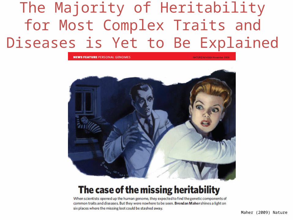
The Majority of Heritability for Most Complex Traits and Diseases is Yet to Be Explained
Maher (2009) Nature
Places the Missing Heritability Could be Hiding
• In the form of common variants of small effect scattered across the genome
• In the form of low frequency variants only partially tagged by common variants
• Estimates of heritability from twin models are inflated (GASP!!!)
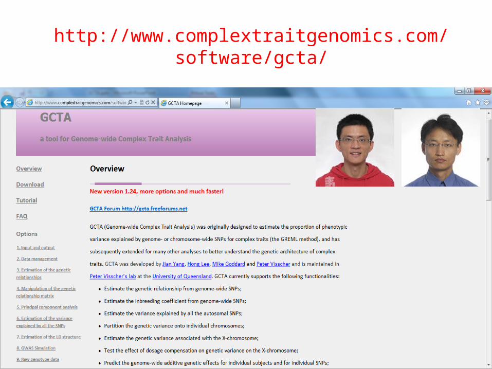
http://www.complextraitgenomics.com/software/gcta/

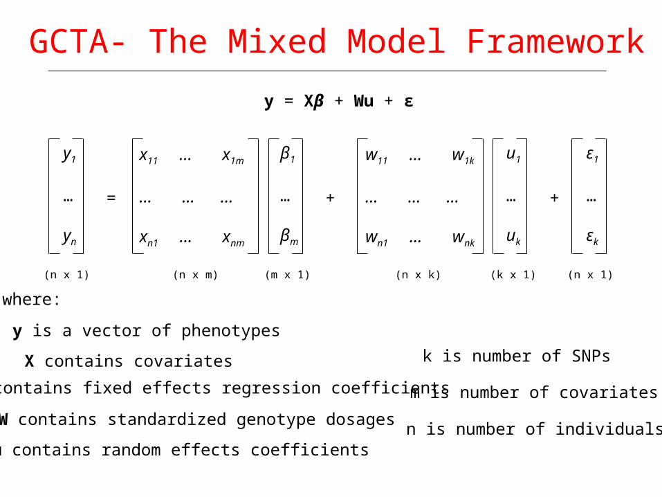
GCTA- The Mixed Model Framework
y = Xβ + Wu + ε
y1
…
yn
=
x11 … x1m
… … …
xn1 … xnm
β1
…
βm
+
w11 … w1k
… … …
wn1 … wnk
u1
…
uk
+
ε1
…
εk
(n x 1) (n x m) (m x 1) (n x k) (k x 1) (n x 1)
n is number of individuals
m is number of covariates
k is number of SNPs
where:
β contains fixed effects regression coefficients
W contains standardized genotype dosages
y is a vector of phenotypes
X contains covariates
u contains random effects coefficients
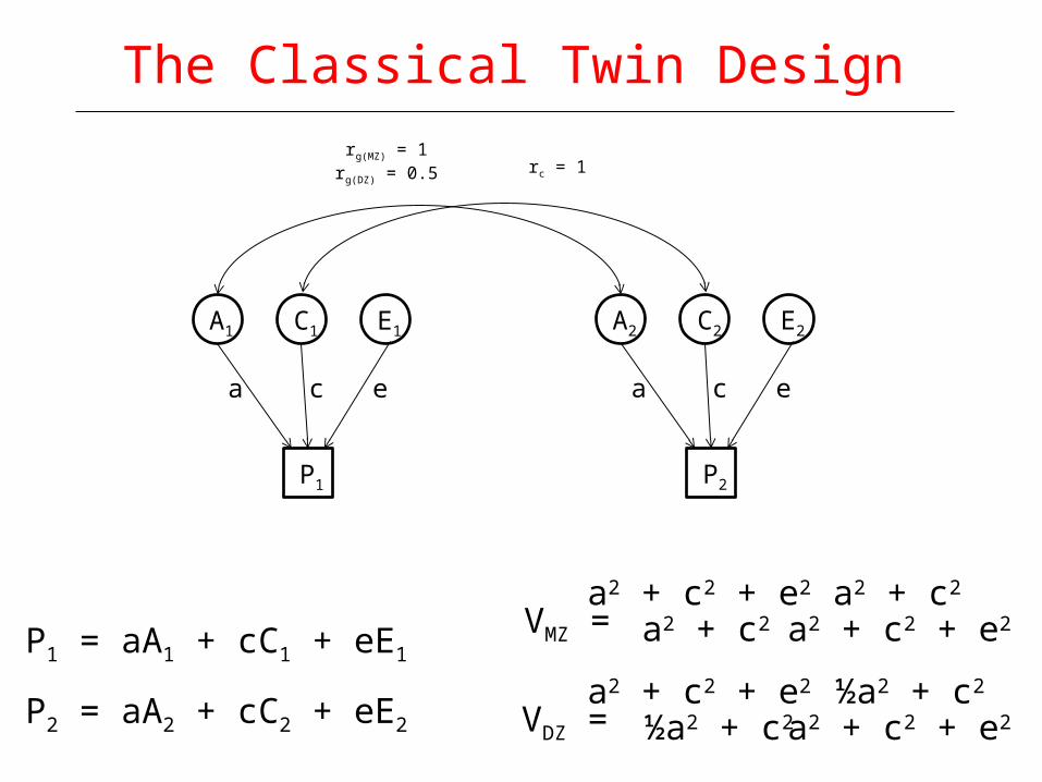
The Classical Twin Design
A1 C1 E1
P1
a ec
A2 C2 E2
P2
a ec
rg(MZ) = 1rg(DZ) = 0.5 rc = 1
VMZ = a2 + c2 + e2
a2 + c2 + e2 a2 + c2a2 + c2
VDZ = a2 + c2 + e2
a2 + c2 + e2 ½a2 + c2½a2 + c2
P1 = aA1 + cC1 + eE1
P2 = aA2 + cC2 + eE2
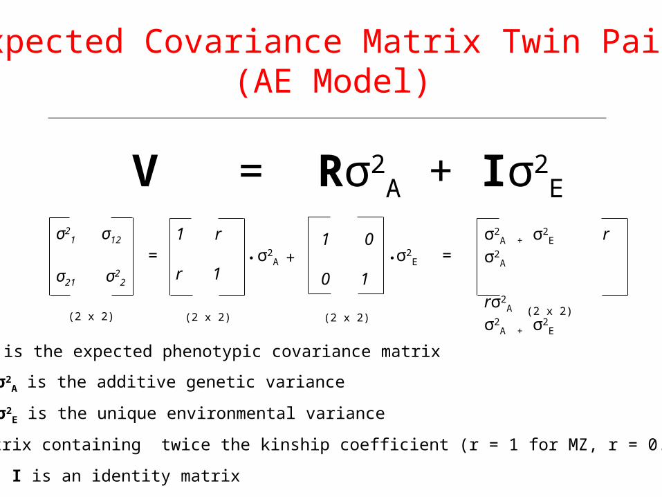
Expected Covariance Matrix Twin Pairs(AE Model)
V = Rσ2A + Iσ2
E
σ21 σ12
σ21 σ22
(2 x 2)
=1 r
r 1
(2 x 2)
+1 0
0 1
σ2A σ2
E. .
(2 x 2)
=σ2
A + σ2E r σ2
A
rσ2A σ2
A + σ2E
(2 x 2)
V is the expected phenotypic covariance matrix
σ2A is the additive genetic variance
σ2E is the unique environmental variance
R is a matrix containing twice the kinship coefficient (r = 1 for MZ, r = 0.5 for DZ))
I is an identity matrix
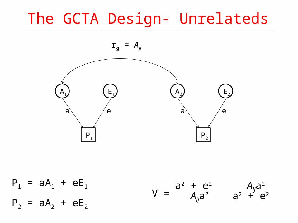
The GCTA Design- Unrelateds
A1 E1
P1
a e
A2 E2
P2
a e
rg = Aij
V = a2 + e2
a2 + e2 Aija2 Aija2P1 = aA1 + eE1
P2 = aA2 + eE2
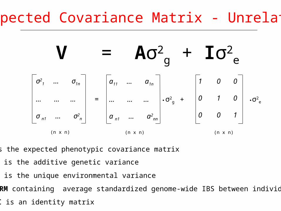
Expected Covariance Matrix - Unrelateds
σ21 … σ1n
… … …
σ n1 … σ2n
(n x n)
=
a11 … a1n
… … …
a n1 … a2nn
(n x n)
+
1 0 0
0 1 0
0 0 1
(n x n)
σ2g σ2
e. .
V = Aσ2g + Iσ2
e
V is the expected phenotypic covariance matrix
σ2g is the additive genetic variance
σ2e is the unique environmental variance
A is a GRM containing average standardized genome-wide IBS between individual i and j
I is an identity matrix
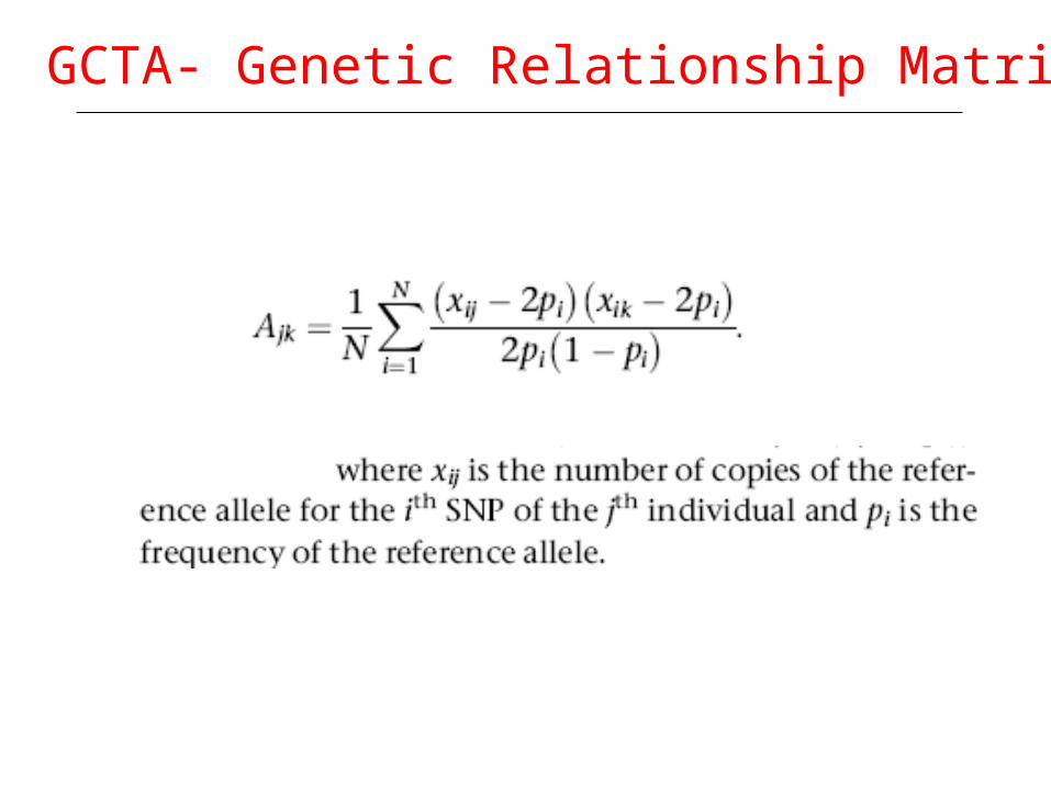
GCTA- Genetic Relationship Matrix
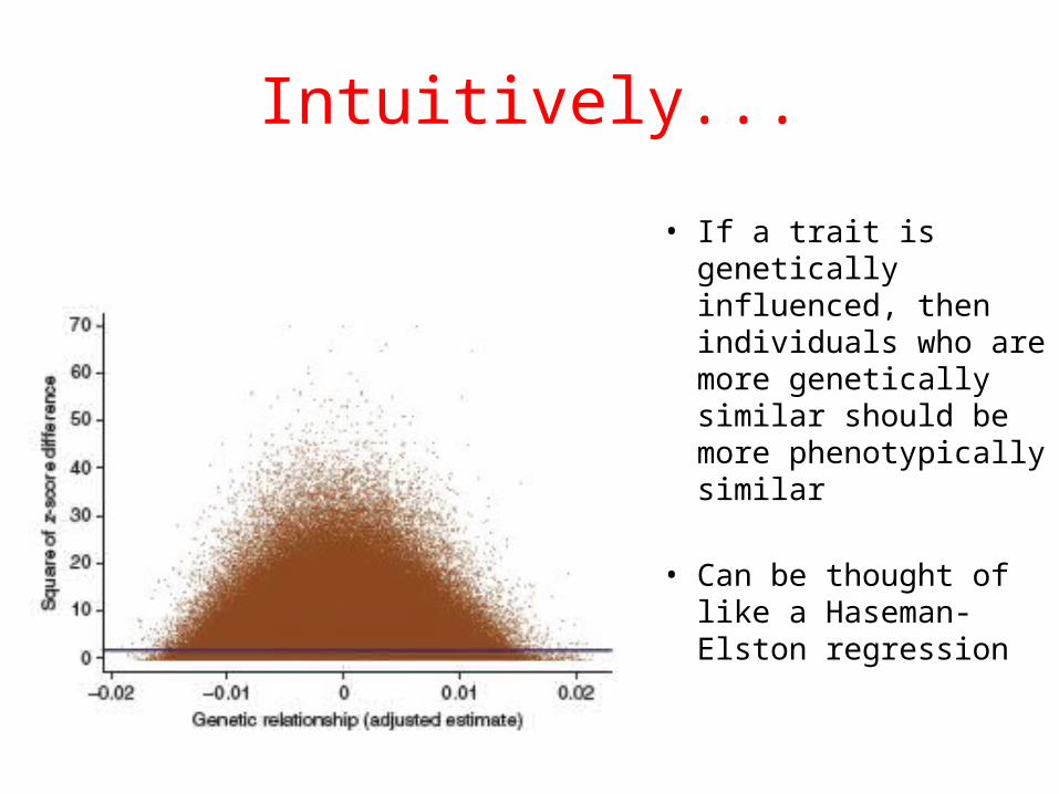
Intuitively...
• If a trait is genetically influenced, then individuals who are more genetically similar should be more phenotypically similar
• Can be thought of like a Haseman- Elston regression
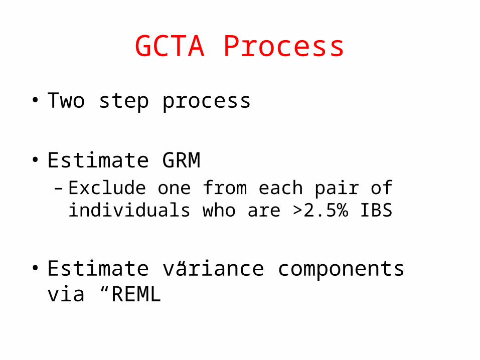
GCTA Process
• Two step process
• Estimate GRM– Exclude one from each pair of individuals who are
>2.5% IBS
• Estimate variance components via “REML”
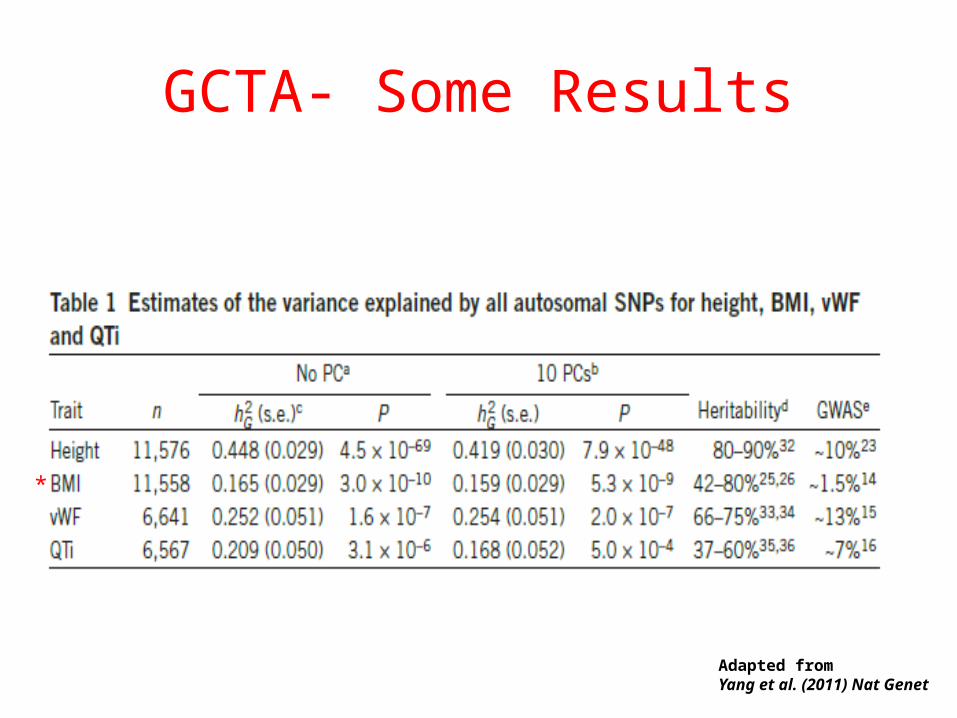
GCTA- Some Results
Adapted from Yang et al. (2011) Nat Genet
*
GCTA Interpretation
• GCTA does not estimate “heritability”
• GCTA does not estimate the proportion of trait variance due to common SNPs
• GCTA tells you nothing definitive about the number of variants influencing a trait, their size or their frequency
GCTA- Some Assumptions
• The GRM accurately reflects the underlying causal variants
• Underlying variants explain the same amount of variance– Relationship between MAF and effect size
• Independent effects– Contributions to h2 overestimated by causal
variants in regions of high LD and underestimated in regions of low LD
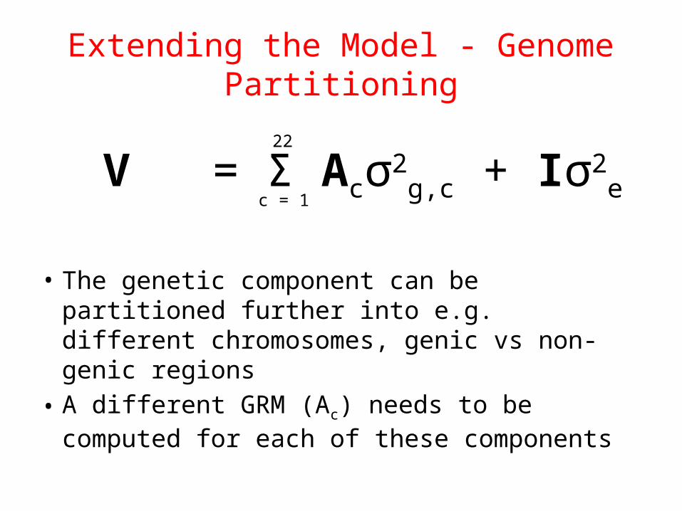
Extending the Model - Genome Partitioning
• The genetic component can be partitioned further into e.g. different chromosomes, genic vs non-genic regions
• A different GRM (Ac) needs to be computed for each of these components
V = Σ Acσ2g,c + Iσ2
ec = 1
22
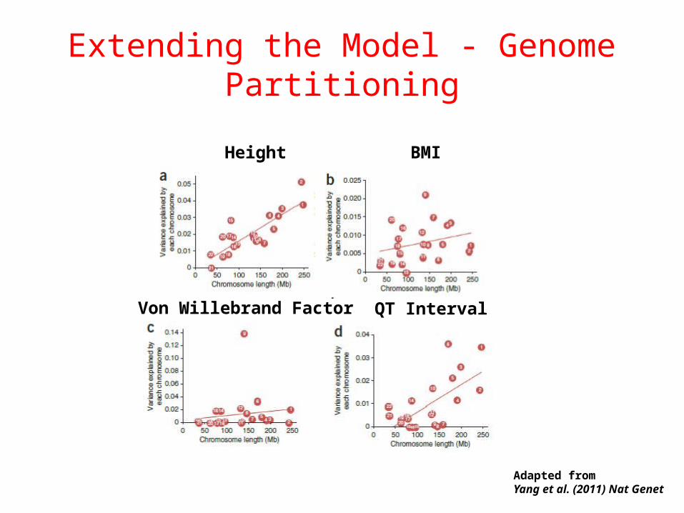
Extending the Model - Genome Partitioning
Height BMI
Von Willebrand Factor QT Interval
Adapted from Yang et al. (2011) Nat Genet
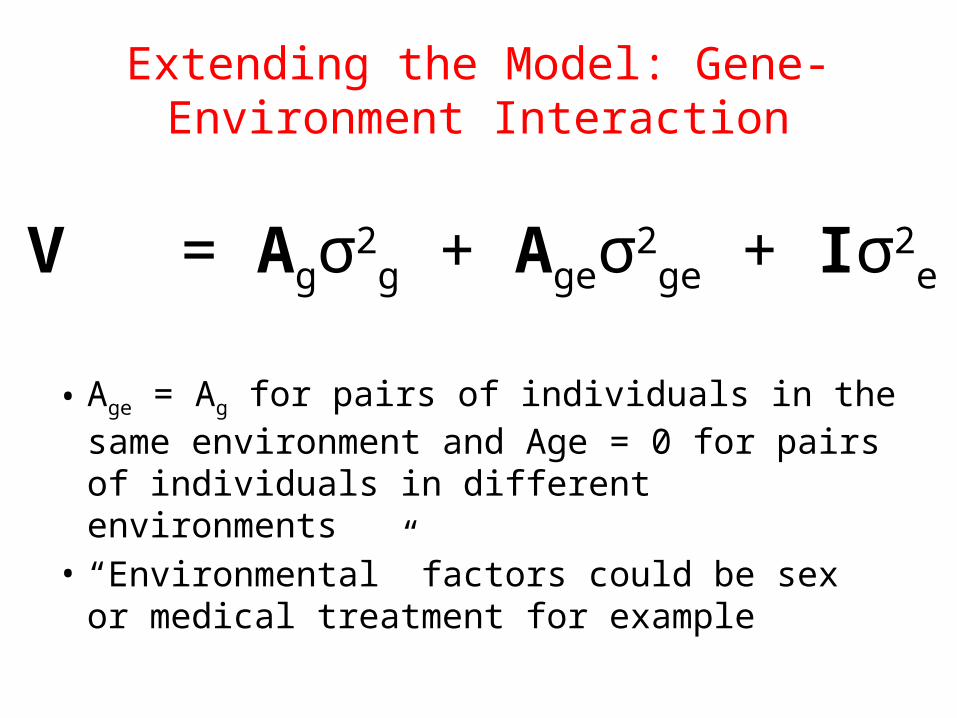
Extending the Model: Gene-Environment Interaction
• Age = Ag for pairs of individuals in the same environment and Age = 0 for pairs of individuals in different environments
• “Environmental” factors could be sex or medical treatment for example
V = Agσ2g + Ageσ2
ge + Iσ2e
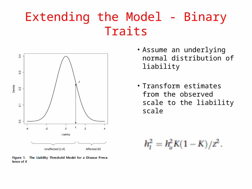
Extending the Model - Binary Traits• Assume an underlying
normal distribution of liability
• Transform estimates from the observed scale to the liability scale
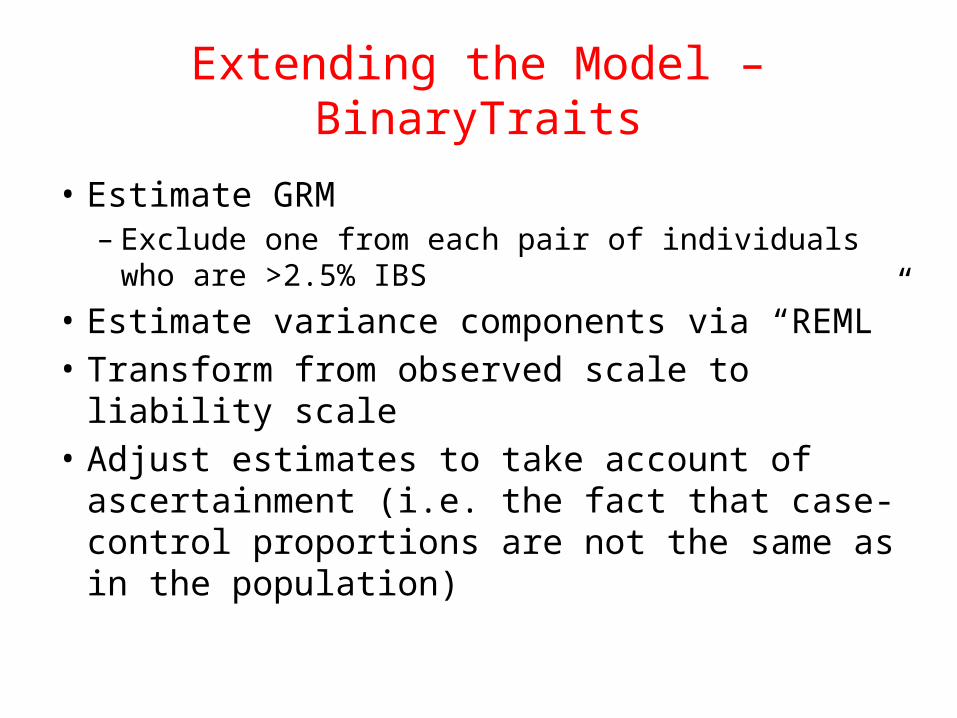
Extending the Model – BinaryTraits
• Estimate GRM– Exclude one from each pair of individuals who are
>2.5% IBS• Estimate variance components via “REML”• Transform from observed scale to liability scale• Adjust estimates to take account of
ascertainment (i.e. the fact that case-control proportions are not the same as in the population)
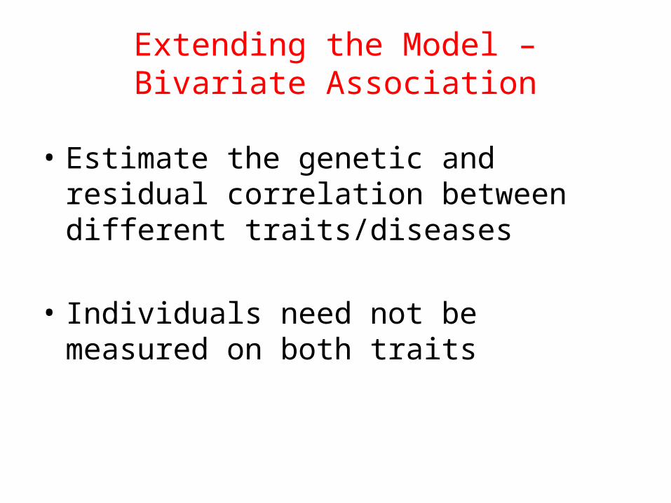
Extending the Model – Bivariate Association
• Estimate the genetic and residual correlation between different traits/diseases
• Individuals need not be measured on both traits
1 4
2 41 3
31
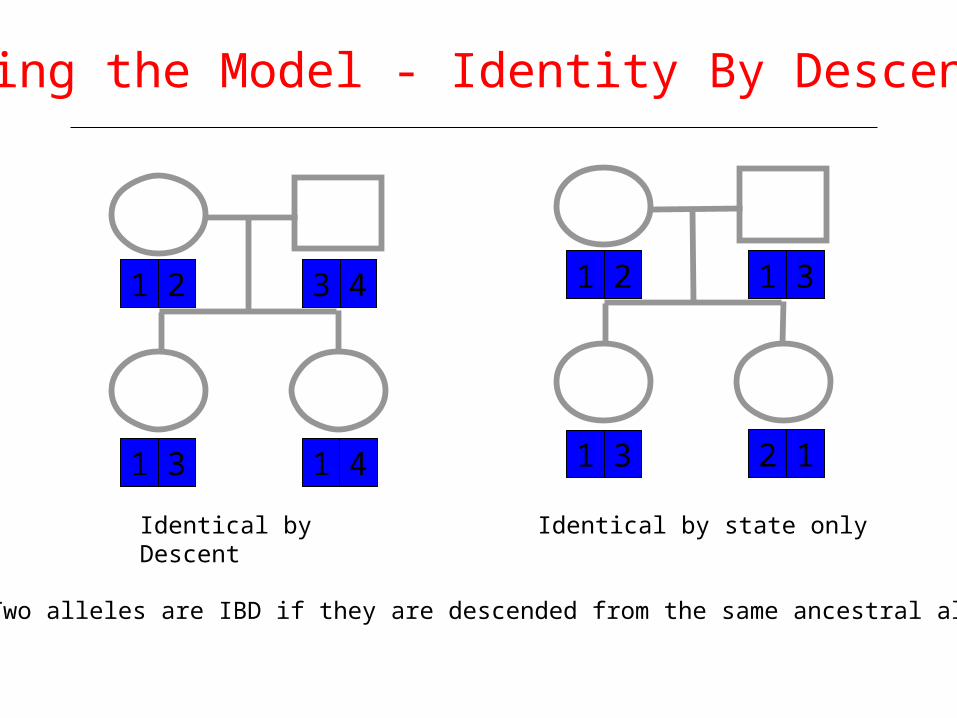
Identical by Descent
2 1
2 31 1
31
Identical by state only
Two alleles are IBD if they are descended from the same ancestral allele
Extending the Model - Identity By Descent (IBD)
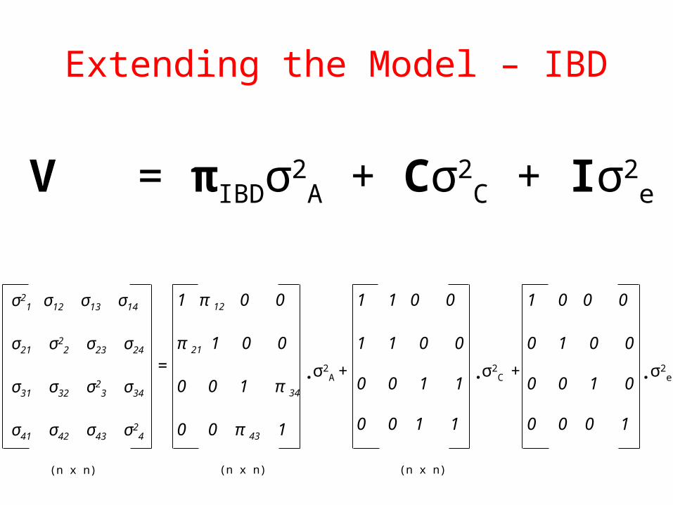
Extending the Model – IBD
V = πIBDσ2A + Cσ2
C + Iσ2e
σ21 σ12 σ13 σ14
σ21 σ22 σ23 σ24
σ31 σ32 σ23 σ34
σ41 σ42 σ43 σ24
(n x n)
= +σ2A.
1 π 12 0 0
π 21 1 0 0
0 0 1 π 34
0 0 π 43 1
(n x n)
.
1 1 0 0
1 1 0 0
0 0 1 1
0 0 1 1
(n x n)
σ2C .
1 0 0 0
0 1 0 0
0 0 1 0
0 0 0 1
σ2e+
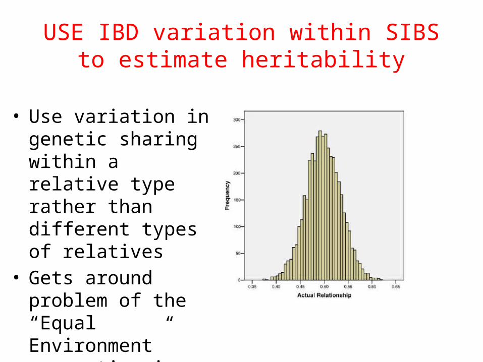
USE IBD variation within SIBS to estimate heritability
• Use variation in genetic sharing within a relative type rather than different types of relatives
• Gets around problem of the “Equal Environment” assumption in twin studies
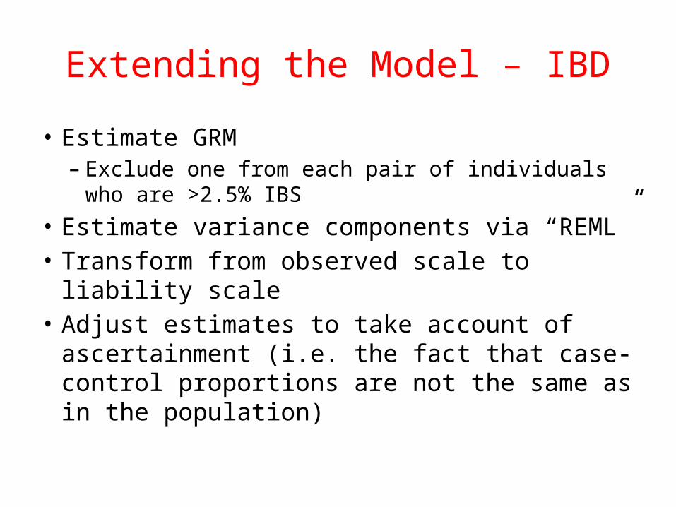
Extending the Model – IBD
• Estimate GRM– Exclude one from each pair of individuals who are
>2.5% IBS• Estimate variance components via “REML”• Transform from observed scale to liability scale• Adjust estimates to take account of
ascertainment (i.e. the fact that case-control proportions are not the same as in the population)
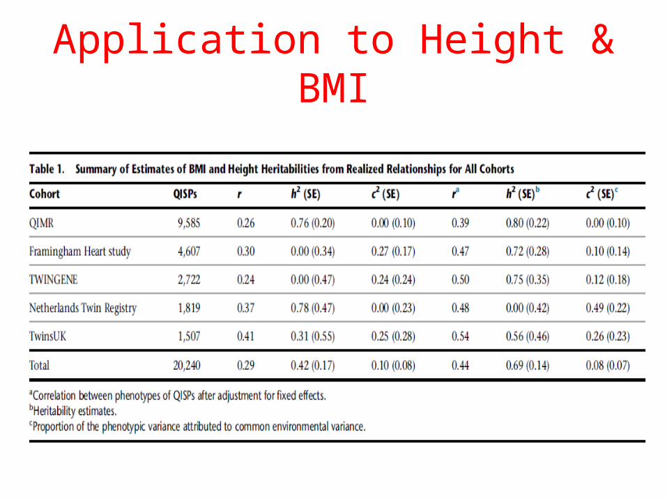
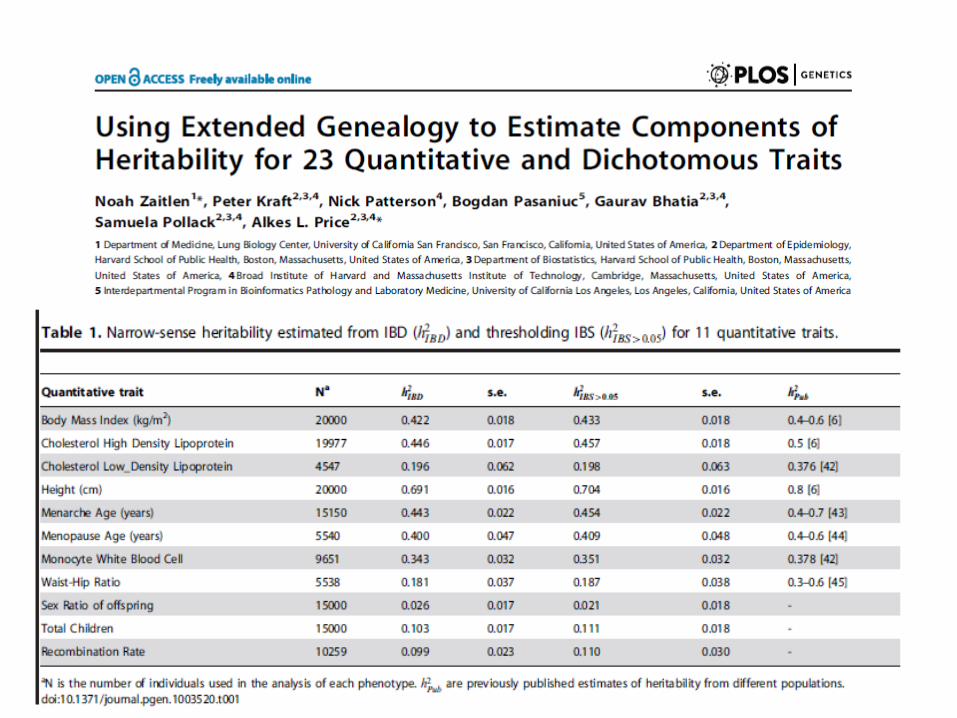
Application to Height & BMI
Idea…
• It should be obvious now, that pretty much all the models that we have touched on this week can be expressed within this GCTA framework
• Yet only a small proportion of these have been parameterized in GCTA
• Considerable scope exists for parameterization of the GCTA framework in Mx…


