================

Estimating Panel Data Models in thePresence of Endogeneity and Selection

Anastasia SemykinaDepartment of EconomicsFlorida State University

Tallahassee, FL 32306-2180asemykina@fsu.edu

Jeffrey M. WooldridgeDepartment of EconomicsMichigan State University

East Lansing, MI 48824-1038wooldri1@msu.edu

This version: May 2, 2008

1

Abstract

We consider estimation of panel data models with sample selection when the equation

of interest contains endogenous explanatory variables as well as unobserved heterogeneity.

We offer a detailed analysis of the pooled two-stage least squares (pooled 2SLS) and fixed

effects-2SLS (FE-2SLS) estimators and discuss complications in correcting for selection

biases that arise when instruments are correlated with the unobserved effect. Assuming

that appropriate instruments are available, we propose several tests for selection bias

and two estimation procedures that correct for selection in the presence of endogenous

regressors. The first correction procedure is valid under the assumption that the errors

in the selection equation are normally distributed, while the second procedure drops

the normality assumption and estimates the model parameters semiparametrically. In

the proposed testing and correction procedures, the error terms may be heterogeneously

distributed and serially dependent in both selection and primary equations. Correlation

between the unobserved effects and explanatory and instrumental variables is permitted.

To illustrate and study the performance of the proposed methods, we apply them to

estimating earnings equations for females using the Panel Study of Income Dynamics

data and perform Monte Carlo simulations.

Keywords: Fixed Effects, Instrumental Variables, Sample Selection, Mills Ratio, Semi-

parametric

2

1 Introduction

Due to the increased availability of longitudinal data and recent theoretical advances,

panel data models have become widely used in applied work in economics. Common

panel data methods account for unobserved heterogeneity characterizing economic agents,

something not easily done with pure cross-sectional data.

In many applications of panel data, particularly when the cross-sectional unit is a

person, family, or firm, the panel data set is unbalanced. That is, the number of time

periods differs by cross-sectional unit. Standard methods such as fixed effects and ran-

dom effects are easily modified to allow unbalanced panels, but simply implementing the

algebraic modifications begs an important question: Why is the panel unbalanced? If the

missing time periods result from self-selection, applying standard methods may result in

inconsistent estimation.

A number of studies have addressed the problems of heterogeneity and selectivity

under the assumption of strictly exogenous explanatory variables. Verbeek and Nijman

(1992) proposed two kinds of tests of selection bias in panel data models. The first kind of

tests – simple variable addition tests – rely on the assumption of no correlation between

the unobserved effects and explanatory variables. Some of their other tests – Hausman-

type tests – do not require this assumption, although no suggestion is made on how

one can consistently estimate parameters of the model if the hypothesis of no selection

bias is rejected. Wooldridge (1995) proposed test and correction procedures that allow

the unobserved effects and explanators be correlated in both the selection and primary

equations. Distributional assumptions are specified for the error terms in the selection

equation, but not for the errors in the primary equation. The model allows idiosyncratic

errors in both equations be serially correlated and heterogeneously distributed.

A semiparametric approach to correcting for selection bias was suggested by Kyriazi-

3

dou (1997). Both the unobserved effects and selection terms are removed by taking the

difference between any two periods in which the selection index is the same (or, in prac-

tice, “similar”). An important assumption here is that equality of selection indices has

the same effect of selection on the dependent variable in the primary equation. Formally,

it is assumed that idiosyncratic errors in both equations in the two periods are jointly

identically distributed conditional on the explanatory variables and unobserved effects in

both equations – a conditional exchangeability assumption. [The conditional exchange-

ability assumption does not always hold in practice – for example, if variances change

over time. Additionally, identification problems may arise when using Kyriazidou’s esti-

mator. For a detailed discussion of these issues see Dustmann and Rochina-Barrachina

(2007).] Rochina-Barrachina (1999) also uses differencing to eliminate the time-constant

unobserved effect; however, in her model the selection is explicitly modeled rather than

differenced-out. She assumes trivariate normal distribution of the error terms in the

selection and differenced primary equations to derive the selection correction term.

The estimators of Wooldridge (1995), Kyriazidou (1997) and Rochina-Barrachina

(1999) help to resolve the endogeneity issues that arise because of non-zero correlation be-

tween individual unobserved effects and explanatory variables. However, other endogene-

ity biases may arise due to a different factor – a nonzero correlation between explanatory

variables and idiosyncratic errors. Such type of endogeneity can become an issue due to

omission of relevant time-varying factors, simultaneous responses to idiosyncratic shocks,

or measurement error. The resulting biases cannot be removed via differencing or fixed

effects estimation, and hence, require special consideration.

Extensions to allow for endogenous explanatory variables in the primary equation

have been proposed by Vella and Verbeek (1999). In particular, they provide a method

for estimating panel data models with censored endogenous regressors and selection, but

they do not allow for correlation between the unobserved effects and exogenous variables

4

in the primary equation. Additionally, when they have more than one endogenous re-

gressor, their approach generally involves multi-dimensional numerical integration, which

can be computationally demanding. Kyriazidou (2001) considers estimation of dynamic

panel data models with selection. In her model, lags of the dependent variables may

appear in both the primary and selection equations, while all other variables are assumed

to be strictly exogenous. Charlier, Melenberg, van Soest (2001) show that using instru-

mental variables (IV) in Kyriazidou’s (1997) estimator produces consistent estimators in

the presence of endogenous regressors under the appropriate conditional exchangeability

assumption, where the conditioning set includes the instruments and unobserved effects

in the primary and selection equations. Furthermore, they apply this method to esti-

mating housing expenditure by households. Askildsen, Baltagi, and Holmas (2003) use

the same approach when estimating wage elasticity of nurses’ labor supply. A somewhat

different estimation strategy was proposed by Dustmann and Rochina-Barrachina (2007),

who suggest using fitted values in Wooldridge’s (1995) estimator, an IV method with

generated instruments in Kyriazidou’s (1997) estimator, and generalized method of mo-

ments (GMM) in Rochina-Barrachina’s (1999) estimator. 1 They apply these methods

to estimating females’ wage equations. Since starting this research, we have come across

other extensions of Wooldridge’s estimator. Those most closely related to the current

work are Gonzalez-Chapela (2004) and Winder (2004). Gonzalez-Chapela uses GMM

when estimating the effect of the price of recreation goods on females’ labor supply, while

Winder uses instrumental variables to account for endogeneity of some regressors when

estimating females’ earnings equations. Both papers use parametric correction that as-

sumes normality of the error terms in the selection equation. Furthermore, the discussion

of the underlying theory in these two papers is quite brief.

As a separate strand of the literature, Lewbel (2005) proposes an estimator that

1Additional discussion of how first differencing combined with a double index assumption can be usedin the estimation of models with endogenous regressors can be found in Rochina-Barrachina (2000).

5

addresses endogeneity and selection in panel data models under the assumption that

one of explanatory variables is conditionally independent of unobserved heterogeneity

and idiosyncratic errors in both primary and selection equations and is conditionally

continuously distributed on a large support. The approach employs weighting to address

selection and removes fixed effects via differencing. The estimator is a two stage least

squares or GMM estimator on the transformed data.

In this study we contribute to the existing literature in several ways. First, we consider

two commonly known estimators used in panel data models with endogenous regressors:

the pooled two-stage least squares (pooled 2SLS) estimator and fixed effects-2SLS (FE-

2SLS) estimator. We show how the presence of unobserved heterogeneity in the selection

and primary equation may complicate selection bias correction when the unobserved effect

is correlated with exogenous variables. Among other things, our analysis demonstrates

that applying cross-sectional correction techniques (such as, for example, the nonpara-

metric estimator of Das, Newey and Vella, 2003) to panel data produces inconsistent

estimators, unless one is willing to make a strong assumption that instruments are uncor-

related with (or even independent of) the unobserved heterogeneity.

We propose simple variable addition tests that can be used to detect endogeneity of

the sample selection process. These tests, which use functions of the selection indicators

from other time periods, can detect correlation between the idiosyncratic error at time

t and selection in other time periods. In contrast to Verbeek and Nijman (1992), the

proposed tests are robust to the presence of arbitrary correlation between unobserved

heterogeneity and explanatory variables. Furthermore, we consider testing for contem-

poraneous selection bias when enough exogenous variables are observed in every time

period. Testing for selection bias is an important first step in analyzing an unbalanced

panel because, while one wants to guard against selection bias, selection correction pro-

cedures tend to reduce the precision of estimated parameters. Applicability of the tests

6

described in Verbeek and Nijman (1992) and Wooldridge (1995) is limited because they

do not allow for endogenous regressors; they may conclude there is selection bias even if

there is none. Our tests are based on the FE-2SLS estimation method, which accounts

for endogeneity of regressors in the primary equation, as well as correlated unobserved

heterogeneity.

In the case when the test does not reject the hypothesis of no selection bias, we suggest

using the FE-2SLS estimator, as it is robust to any type of correlation between unobserved

effects and explanatory and instrumental variables, does not require specification of the

reduced form equations for endogenous variables, and makes no assumptions of errors

distribution.(More efficient GMM estimation is always a possibility, too.) If the hypothesis

of no selection bias is rejected, we propose selection correction based on the pooled 2SLS

estimator.

We propose two approaches that consider the estimation of population parameters in

the presence of endogenous regressors and selection. The first approach is parametric and

it uses assumptions that are akin to those specified in Wooldridge (1995). In particular,

we assume normality of the errors in the selection equation, and linear conditional mean

of the error in the primary equation to derive the correction term. As an alternative

approach, we propose a semiparametric estimator that makes no distributional assump-

tions in the selection and primary equations. Within this approach, the correction term

is estimated semiparametrically using series estimators. Both estimators permit hetero-

geneously distributed and serially dependent errors in the selection equation. Similarly,

time heteroskedasticity and arbitrary serial correlation are permitted in the primary equa-

tion. Thus, our approach is complementary to Kyriazidou’s method (Kyriazidou, 1997) in

that our methods allow for arbitrary dynamics in the errors of both equations. Moreover,

our semiparametric estimator does not rely on distributional assumptions as in Rochina-

Barrachina (1999), and it does not require the availability of a conditionally independent

7

variable as in Lewbel (2005).

We apply our methods to Panel Study of Income Dynamics (PSID) data, using the

years 1980 to 1992. Similarly to Dustmann and Rochina-Barrachina (2007), we estimate

earnings equations for females. The finite sample properties of the test and proposed

estimators are studied via Monte Carlo simulations.

2 Consistency of Pooled 2SLS

We begin with analyzing the assumptions under which the pooled 2SLS estimator applied

to an unbalanced panel is consistent. At this point, we do not explicitly model unobserved

heterogeneity, but rather leave it as a part of an error term. Specifically, the main equation

of interest is

yit = xitβ + vit, t = 1, . . . , T (1)

where xit is a 1 × K vector that contains both exogenous and endogenous explanatory

variables, β is a K×1 vector of parameters, and vit is the error term. Additionally, assume

there exists a 1 × L vector of instruments (L ≥ K), zit, such that the contemporaneous

exogeneity assumption holds for all variables in zit: E(vit|zit) = 0, t = 1, . . . , T . Unless

stated otherwise, vectors xit and zit always contain an intercept. Instruments are assumed

to be sufficiently partially correlated with the explanatory variables in the population

analog of equation (1). In fact, zit includes all the variables in xit that are exogenous in

(1). Under the specified assumptions the pooled 2SLS estimator on a balanced panel is

consistent.

As a next step, we introduce selection (or incidental truncation) into the model. Let

sit be a selection indicator, which equals one if (yit, xit, zit) is observed, and zero otherwise.

8

Then the pooled 2SLS estimator on an unbalanced panel is

β2SLS = β +

(N−1

N∑i=1

T∑t=1

sitx′itzit

) (N−1

N∑i=1

T∑t=1

sitz′itzit

)−1

×(

N−1

N∑i=1

T∑t=1

sitz′itxit

)]−1 (N−1

N∑i=1

T∑t=1

sitx′itzit

)

×(

N−1

N∑i=1

T∑t=1

sitz′itzit

)−1 (N−1

N∑i=1

T∑t=1

sitz′itvit

). (2)

For fixed T with N → ∞, we can essentially read off conditions that are sufficient for

consistency of the pooled 2SLS estimator. These conditions extend those in Wooldridge

(2002, Section 17.2.1) for the pure cross sectional case. We summarize with a set of as-

sumptions and a proposition.

ASSUMPTION 2.1: (i) (yit, xit, zit) is observed whenever sit = 1; (ii) E(vit|zit, sit) = 0,

t = 1, . . . , T ; (iii) rank E(∑T

t=1 sitz′itxit

)= K; (iv) rank E

(∑Tt=1 sitz

′itzit

)= L.

PROPOSITION 2.1: Under Assumption 2.1 and standard regularity conditions, the

pooled 2SLS estimator is consistent and√

N -asymptotically normal for β.

Assumption 2.1(iv) imposes nonsingularity on the outer product of the instrument

matrix in the selected sample. Typically, it is satisfied unless instruments are redundant or

the selection mechanism selects too small a subset of the population. Assumption 2.1(iii)

is the important rank condition – again, on the selected subpopulation – that requires

that we have enough instruments (L ≥ K) and that they are sufficiently correlated with

xit. Any exogenous variable in xit would be included in zit.

Assumption 2.1(ii) is the sense in which selection is assumed to be exogenous in (2).2

2As is seen from equation (2), a weaker sufficient condition, E(sitz′itvit) = 0, can be used instead of

9

It requires that vit is conditionally mean independent of zit and selection in time period

t. This assumption will be violated if sit is correlated with vit, including cases where vit

contains a time-constant unobserved effect that is related to selection. As we will see

in Section 5, often an augmented equation will satisfy Assumption 2.1(ii) even when the

original population model does not, in which case we can apply pooled 2SLS directly to

the augmented equation (provided we have sufficient instruments). Assumption 2.1(ii) is

silent on the relationship between vit and sir, r 6= t. In other words, selection is assumed to

be contemporaneously exogenous but not strictly exogenous. Consequently, consistency

of the pooled 2SLS estimator can hold even if yit reacts to selection in the previous

time period, si,t−1, or if selection next period, si,t+1, reacts to unexpected changes in yit

(as measured by vit). Of course, if vit contains time-constant unobserved heterogeneity

that is correlated with sit, then sir is likely to be correlated with vit, too. Similarly,

if instruments are correlated with omitted unobserved heterogeneity, Assumption 2.1(ii)

will fail. Nevertheless, in Section 5 we will put Proposition 2.1 to good use in models

with unobserved heterogeneity that is correlated with both instrumental variables and

selection.

Importantly, Proposition 2.1 does not impose restrictions on the nature of the endoge-

nous elements of xit. For example, we do not need to assume reduced forms linear in zit

with additive, independent, or even zero conditional mean, errors. Consequently, Propo-

sition 2.1 can apply to binary endogenous variables or other variables with discreteness in

their distributions. The rank condition Assumption 2.1(iii) can hold quite generally, and

is essentially a restriction on the linear projection of xit on zit in the selected subpopula-

tion.

Assumption 2.1(ii). Here, we focus on the conditional mean assumption, as selection correction and testswill be based on that assumption.

10

3 FE-2SLS and Simple Variable Addition Tests

In many applications of panel data methods, we want to include unobserved heterogeneity

in the equation that can be correlated with explanatory variables, and even instrumental

variables. In this and subsequent sections we explicitly model the error term as a sum of

an unobserved effect and an idiosyncratic error. Therefore, the model is now

yit = xitβ + ci + uit, t = 1, . . . , T, (3)

where ci is the unobserved effect and uit are the idiosyncratic errors. We allow for arbitrary

correlation between the unobserved effect and explanatory variables. In addition, we

allow some elements of xit to be correlated with the idiosyncratic error, uit, as occurs in

simultaneous equations models, measurement error, and time-varying omitted variables.

In order to allow for correlation between the regressors and the idiosyncratic errors, we

assume the existence of instruments, zit, which are strictly exogenous conditional on

ci. This permits for unspecified correlation between zit and ci, but requires zit to be

uncorrelated with uir : r = 1, ..., T. The dimensions of xit and zit are the same as in the

previous section, but, since the FE estimator involves time-demeaning, we assume that

all variables in xit and zit are time-varying.

We want to determine assumptions under which ignoring selection will result in a

consistent estimator. For each i and t, define xit≡xit − T−1i

∑Tr=1 sirxir, where Ti =

11

∑Tt=1 sit, and similarly for zit, yit. Then the FE-2SLS estimator can be written as

βFE−2SLS =

(N−1

N∑i=1

T∑t=1

sitx′itzit

)(N−1

N∑i=1

T∑t=1

sitz′itzit

)−1

×(

N−1

N∑i=1

T∑t=1

sitz′itxit

)]−1 (N−1

N∑i=1

T∑t=1

sitx′itzit

)

×(

N−1

N∑i=1

T∑t=1

sitz′itzit

)−1 (N−1

N∑i=1

T∑t=1

sitz′ityit

), (4)

which, using straightforward algebra, can be shown to be equal to

β +

(N−1

N∑i=1

T∑t=1

sitx′itzit

)(N−1

N∑i=1

T∑t=1

sitz′itzit

)−1

×(

N−1

N∑i=1

T∑t=1

sitz′itxit

)]−1 (N−1

N∑i=1

T∑t=1

sitx′itzit

)

×(

N−1

N∑i=1

T∑t=1

sitz′itzit

)−1 (N−1

N∑i=1

T∑t=1

sitz′ituit

). (5)

The benefit of the within transformation is that it removes the unobserved effect, ci. Of

course, it also means that we cannot estimate coefficients on any time-constant explana-

tory variables.

Denote zi = (zi1, . . . , ziT ) and si = (si1, . . . , siT ). For consistency of the FE-2SLS

estimator on an unbalanced panel, we make the following assumptions:

ASSUMPTION 3.1: (i) (yit, xit, zit) is observed whenever sit = 1; (ii) E(uit|zi, si, ci) =

0, t = 1, . . . , T ; (iii) rank E(∑T

t=1 sitx′itzit

)= K; (iv) rank E

(∑Tt=1 sitz

′itzit

)= L.

PROPOSITION 3.1: Under Assumption 3.1 and standard regularity conditions, the

FE-2SLS estimator is consistent and√

N -asymptotically normal for β.

12

Assuming we have sufficient time-varying instruments, Assumption 3.1(ii) is the crit-

ical assumption. By iterated expectations, 3.1(ii) guarantees that E(∑T

t=1 sitz′ituit

)= 0.

Thus, the last term in equation (5) converges to zero in probability as N →∞.

Assumption 3.1(ii) always holds if the zit are strictly exogenous, conditional on ci,

and the sit are completely random – so that si is independent of (uit, zi, ci) in all periods.

It also holds when sit is a deterministic function of (zi, ci) for all t. In either case we

have E(uit|zi, si, ci) = E(uit|zi, ci) = 0, t = 1, . . . , T . Allowing for arbitrary correlation

between sit and ci is why fixed effects methods are attractive for unbalanced panels when

one suspects different propensities to attrit or otherwise select out of the sample based on

unobserved heterogeneity. Random effects (RE) estimation would require, in addition to

3.1(ii), E(ci|zi, si) = 0, and so RE is not preferred to fixed effects unless selection is truly

exogenous.

Allowing for arbitrary correlation between sit and ci does come at a price. In par-

ticular, Assumption 3.1(ii) is not strictly weaker than Assumption 2.1(ii) because 3.1(ii)

requires that uit is uncorrelated with selection indicators in all time periods. If we ap-

ply Assumption 2.1(ii) to the current context, the pooled 2SLS estimator is consistent if

E(ci + uit|zit, sit) = 0. Granted, with the presence of ci, it is unlikely that 2.1(ii) would

hold when 3.1(ii) does not. But, without an unobserved effect – for example, in a model

with a lagged dependent variable and no unobserved effect – 2.1(ii) becomes much more

plausible than 3.1(ii). The distinctions between these two assumptions will surface again

in Section 5.

Inference for the FE-2SLS estimator on the unbalanced panel can be carried out

using standard statistics or, even better, statistics that are robust to heteroskedasticity

and serial correlation in uit : t = 1, ..., T. See Wooldridge (1995) for the case of strictly

exogenous regressors; the arguments are very similar.

13

Assumption 3.1 suggests some simple variable addition tests for selection bias. Be-

cause Assumption 3.1(ii) implies that uit is uncorrelated with sir for all t and r, we can

add time-varying functions of the selection indicators as explanatory variables and obtain

simple t or joint Wald tests. For example, we can add si,t−1 or si,t+1 to (3) and test

their significance; we lose a time period (either the first or last) in doing so. Two other

possibilities are∑t−1

r=1 sir (the number of times in the sample prior to time period t) and∑T

r=t+1 sir (the number of times in the sample after time period t). For cases of attrition,

where attrition is an absorbing state, neither si,t−1 or∑t−1

r=1 sir varies across i for the se-

lected sample, so they cannot be used to test for attrition bias. But si,t+1 and∑T

r=t+1 sir

can be used to test for attrition bias.

Adding functions of the selection indicators from other time periods is simple and

should have power for detecting selection mechanisms that cause inconsistency in the

FE-2SLS estimator. Insofar as the selection indicators are correlated over time, the tests

described here will have some ability to detect contemporaneous selection. However, cor-

relation between sit and uit cannot be directly tested by adding selection indicators in

an auxiliary regression: it never makes sense to add sit at time t because, by definition,

sit = 1 for all t in the selected sample. The next section allows us to test for contempo-

raneous correlation between uit and sit if the set of exogenous instrumental variables is

observed in each time period.

14

4 Testing for Selection Bias Under Incidental Trun-

cation

One way to test for contemporaneous selection bias is to model E(vit|zit, sit) in equation

(1). We could then estimate the equation with the additional term inserted and test

for selection using the t-test or the Wald test. This type of test has been proposed by

Verbeek and Nijman (1992) for panel data models with exogenous explanatory variables.

However, if vit includes an unobserved effect, we might conclude there is selection bias

simply because the unobserved effect is correlated with some explanatory variables. Here,

we build on the test proposed by Wooldridge (1995), which tests for selection bias after

estimation by fixed effects. In particular, we extend this approach to allow the possibility

that some explanatory variables are not strictly exogenous even after we remove the

unobserved effect.

Because fixed effects methods allow selection to be correlated with unobserved hetero-

geneity, it has advantages over random effects methods. Our approach here is to assume

that, in the absence of evidence to the contrary, a researcher applies fixed effects 2SLS to

an unbalanced panel. The goal is to then test whether there is sample selection correlated

with the idiosyncratic error in the primary equation.

To accommodate specific models of selection, we change the notation slightly from

the previous section and write the primary equation as

yit1 = xitβ1 + ci1 + uit1, t = 1, . . . , T, (6)

where xit is a 1×K vector of explanatory variables (some of which can be endogenous),

β1 is a K×1 vector of parameters, ci1 is the unobserved effect and uit1 is the idiosyncratic

error. Let zit still denote a 1 × L vector of instruments, which are strictly exogenous

15

conditional on ci1. It is assumed that both xit and zit contain an intercept. In most panel

data models, different time intercepts are usually implicit. Unlike in the previous section

we now assume that the instrumental variables zit are always observed, while (yit1, xit1)

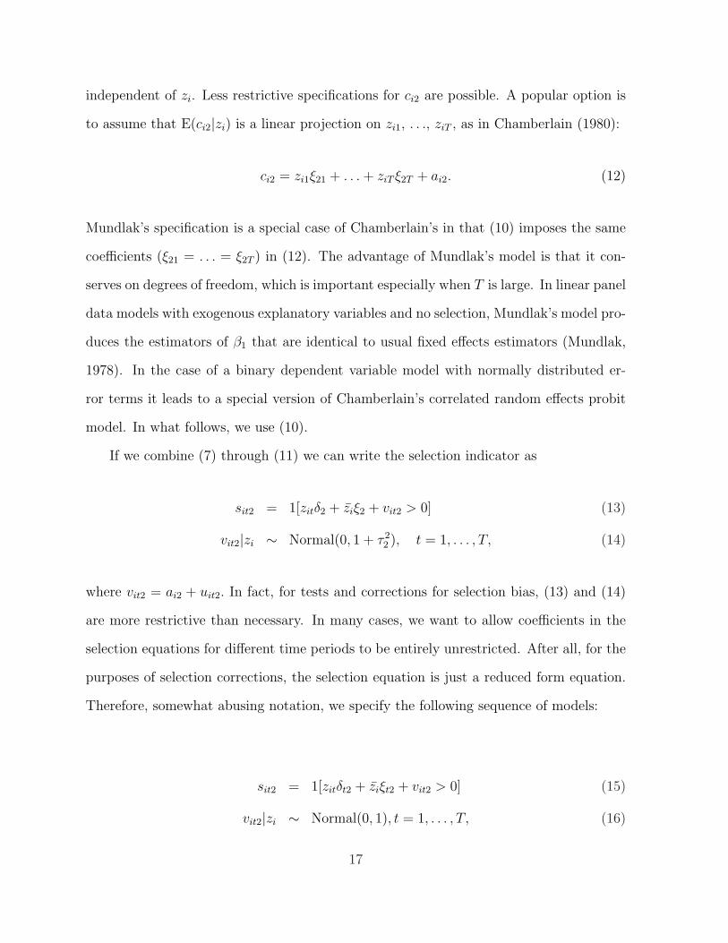
are only observed when the selection indicator, now denoted sit2, is unity. To obtain a

test it is convenient to define a latent variable, s∗it2,

s∗it2 = zitδ2 + ci2 + uit2, t = 1, . . . , T. (7)

Here ci2 is an unobserved effect and uit2 is an idiosyncratic error. The selection indicator,

sit2, is generated as

sit2 = 1[s∗it2 > 0] = 1[zitδ2 + ci2 + uit2 > 0], (8)

where 1[·] is the indicator function. We will derive a test under the assumption

uit2|zi, ci2∼Normal(0, 1), t = 1, . . . , T, (9)

so that sit2 follows an unobserved effects probit model. We allow arbitrary serial depen-

dence in uit2.To proceed further, we model the relationship between the unobserved effect, ci2, and

the strictly exogenous variables, zi. We use the modeling device as in Mundlak (1978). In

particular, assume that the unobserved effect can be modeled as

ci2 = ziξ2 + ai2, (10)

ai2|zi ∼ Normal(0, τ 22 ), t = 1, . . . , T, (11)

which assumes that the correlation between ci2 and zi acts only through the time averages

of the exogenous variables, while the remaining part of the unobserved effect, ai2, is

16

independent of zi. Less restrictive specifications for ci2 are possible. A popular option is

to assume that E(ci2|zi) is a linear projection on zi1, . . ., ziT , as in Chamberlain (1980):

ci2 = zi1ξ21 + . . . + ziT ξ2T + ai2. (12)

Mundlak’s specification is a special case of Chamberlain’s in that (10) imposes the same

coefficients (ξ21 = . . . = ξ2T ) in (12). The advantage of Mundlak’s model is that it con-

serves on degrees of freedom, which is important especially when T is large. In linear panel

data models with exogenous explanatory variables and no selection, Mundlak’s model pro-

duces the estimators of β1 that are identical to usual fixed effects estimators (Mundlak,

1978). In the case of a binary dependent variable model with normally distributed er-

ror terms it leads to a special version of Chamberlain’s correlated random effects probit

model. In what follows, we use (10).

If we combine (7) through (11) we can write the selection indicator as

sit2 = 1[zitδ2 + ziξ2 + vit2 > 0] (13)

vit2|zi ∼ Normal(0, 1 + τ 22 ), t = 1, . . . , T, (14)

where vit2 = ai2 + uit2. In fact, for tests and corrections for selection bias, (13) and (14)

are more restrictive than necessary. In many cases, we want to allow coefficients in the

selection equations for different time periods to be entirely unrestricted. After all, for the

purposes of selection corrections, the selection equation is just a reduced form equation.

Therefore, somewhat abusing notation, we specify the following sequence of models:

sit2 = 1[zitδt2 + ziξt2 + vit2 > 0] (15)

vit2|zi ∼ Normal(0, 1), t = 1, . . . , T, (16)

17

Time varying coefficients on the time average can arise from a standard probit model if

we allow the variance of the idiosyncratic term to change over time or if we make the

effect of ci2 in equation (8) time varying. Typically, there would be some restrictions on

the parameters over time, but we will use the flexibility of (15) and (16) because it is

more robust.

Given the above (nominal) assumptions and some additional ones, we can derive a

test for selection bias. Similar to Wooldridge (1995), suppose (uit1, vi2) is independent

of (zi, ci1), where vi2 = (vi12, . . . , viT2)′, and (uit1, vit2) is independent of (vi12, . . ., vi,t−1,2,

vi,t+1,2, . . ., viT2). Then, if E(uit1|vit2) is linear,

E(uit1|zi, ci1, vi2) = E(uit1|vi2) = E(uit1|vit2) = ρ1vit2, t = 1, . . . , T, (17)

where, for now, we assume a regression coefficient, ρ1, constant across time. Independence

of vi2 and ci1 would not be a good assumption if vi2 contains an unobserved effect, as we

expect, but, at this point, we are using these assumptions to motivate a test for selection

bias. In Section 5 we will be more formal about stating assumptions used for a consistent

correction procedure.

From Assumption 3.1 we know that for the FE-2SLS estimator to be consistent on

an unbalanced panel, it should be that E(uit1|zi, ci1, si2) = 0. If selection is not random,

this expectation will depend on the selection indicators and the zit. Under the previous

assumptions, we can write

E(uit1|zi, ci1, si2) = ρ1E(vit2|zi, ci1, si2) = ρ1E(vit2|zi, sit2), t = 1, ..., T. (18)

Now, we can augment the primary equation as

yit1 = xitβ + ci1 + ρ1E(vit2|zi, sit2) + eit1, t = 1, ..., T, (19)

18

where, by construction, E(eit1|zi, ci1, si2) = 0, t = 1, ..., T. It follows that, if we knew

E(vit2|zi, sit2), then a test for selection bias is obtained by testing H0 : ρ1 = 0 in (19),

which we can estimate by FE-2SLS. Of course, since we are only using observations with

sit2 = 1 we need only find E(vit2|zi, sit2 = 1), and this follows from the usual probit

calculation:

E(vit2|zi, sit2 = 1) = λ(zitδt2 + ziξt2), t = 1, . . . , T, (20)

where λ(·) denotes the inverse Mills ratio. Then the following procedure can be used to

test for sample selection:

PROCEDURE 4.1 (Valid under the null hypothesis, Assumption 3.1):

(i) For each time period, use the probit model to estimate the equation

P(sit2 = 1|zi) = Φ(zitδt2 + ziξt2). (21)

Use the resulting estimates to obtain the inverse Mills ratios, λit2≡λ(zitδt2 + ziξt2).

(ii) For the selected sample, estimate (19) using FE-2SLS, but where λit2 is in place of

E(vit2|zi, sit2). In addition to λit2, we can also add the interactions of the inverse Mills

ratio with time dummies to allow for different correlations between the idiosyncratic

errors uit1 and vit2 (to allow ρ1 be different across t).

(iii) Use the t-statistic for ρ1 to test the hypothesis H0 : ρ1 = 0, or, in the case when the

interactions of the inverse Mills ratio and time dummies are added, use the Wald

test to test joint significance of those terms. The variance matrix robust to serial

correlation and heteroskedasticity should be used.

If the null hypothesis is true, that is, there is no selection problem, then the FE-2SLS

19

estimator is consistent, although this particular test only checks for contemporaneous se-

lection. As we discussed in Section 3, the FE-2SLS estimator is consistent even if there is

arbitrary correlation between the unobserved effect and the instrumental variables, and it

allows selection to be correlated with ci1, too. It does not require us to specify the reduced

form equations for the endogenous variables and it imposes no distributional assumptions

on uit1. Finally, the serial correlation in uit1 is not restricted in any way. Generally, the

test in Procedure 4.1 should be useful for detecting selection at time t that is correlated

with uit1. The tests in Section 3 can be used to determine if selection in time period t is

correlated with the idiosyncratic errors in other time periods – another condition required

for consistency of FE-2SLS.

5 Correcting for Selection Bias

5.1 General Setup

If the test described in Section 4 rejects the hypothesis of no selection bias (that depends

on the idiosyncratic errors), then a selection correction procedure is needed. As noted

earlier, the procedure described in the previous section works for testing, but it can not be

used to correct for selection bias. The main problem is the appearance of an unobserved

effect inside the index of the probit selection model. If an unobserved effect is present

in the selection equation, the error terms in that equation are inevitably serially corre-

lated, which implies a very complicated form for the conditional expectation E(vit2|zi, si2).

(Plus, some of the other assumptions would be unrealistic, too.) Fortunately, provided

we make appropriate linearity assumptions about the conditional expectation of ci1, as

in Chamberlain (1980) and Mundlak (1978), we can obtain a valid selection correction.

20

Specifically, model the unobserved effect as

ci1 = ziξ1 + ai1, (22)

E(ai1|zi) = 0. (23)

This condition is akin to (10) and may seem a bit restrictive. However, it in fact is

very similar in spirit to the traditional fixed effects estimator. As mentioned earlier, im-

posing assumptions (22) and (23) in linear panel data models with exogenous explanatory

variables (xit = zit, t = 1, . . . , T ) produces the estimators of slope parameters that are

identical to fixed-effects estimators when the estimation is performed on a balanced panel

(Mundlak 1978). In equation (22), zi contains all exogenous variables from the original

equation, and hence the effects of those variables in the primary equation are identified

off of their deviations from the individual-specific means. With regard to the endogenous

variables, their coefficients are identified off of the deviations in the instrumental variables

from their within-individual average values. This is very similar to traditional fixed-effects

estimation, where the unobserved heterogeneity is assumed to be time-invariant. Natu-

rally, individual-specific time means of exogenous variables vary with T ; however, this

does not cause a threat to the consistency of the estimator. The asymptotic properties of

the considered estimators are for T fixed with N →∞. Even though the time means are

imprecise and change as the time span changes, the corresponding discrepancies go away

when averaged across individuals.

Another key feature of condition (22) is that the time means of exogenous variables are

obtained on the data that are not distorted by selection (here we exploit the assumption

that zit are observed for all i and t). This is one feature that crucially distinguishes the

proposed estimator from a standard fixed-effects estimator that performs time-demeaning

on a selected sample. While being ideologically similar to fixed effects, the model in (22)

21

and (23) is free of selection biases, which makes it an attractive modeling device.

Given condition (22) and (23), we can plug into (6) and obtain

yit1 = xit1β1 + ziξ1 + ai1 + uit1 = xit1β1 + ziξ1 + vit1, t = 1, . . . , T, (24)

where vit1 ≡ ai1 + uit1 and is mean-independent of zi in the balanced panel. Once we

introduce selection that is correlated with unobserved heterogeneity and idiosyncratic

errors in the primary equation, it is useful to write

yit1 = xit1β1 + ziξ1 + E(vit1|zi, sit2) + eit1, (25)

E(eit1|zi, sit2) = 0, t = 1, . . . , T. (26)

So, if we know E(vit1|zi, sit2), the consistency of the pooled 2SLS estimator would follow

by Proposition 2.1.

Note how we do not assert that E(eit1|zi, si2) = 0; in fact, generally eit1 will be

correlated with selection indicators sir2 for r 6= t. This is an important benefit of the

current approach: we can ignore selection in other time periods that might be correlated

with uit. Equations (25) and (26) also show that applying the Mundlak-Chamberlain

device to the unbalanced panel, even without a selection term, can be consistent even when

the fixed effects estimator is not. Recall that for consistency of the FE-2SLS estimator

on the unbalanced sample, selection must be strictly exogenous conditional on ci1. It is

plausible that vit1 and vit2 might be uncorrelated – so E(vit1|zi, sit2) = 0 – even though

si,t−1,2 is correlated with uit1. If so, FE-2SLS is generally inconsistent but adding zi in

each time period and using pooled 2SLS is consistent. (Of course, this assumes we observe

zit in every time period.)

Generally, equations (25) and (26) show how we can correct for selection by applying

pooled 2SLS to (25), at least once we find E(vit1|zi, sit2). It is possible to make paramet-

22

ric assumptions and find the exact expression for E(vit1|zi, sit2), or use semiparametric

methods. We consider both approaches below.

5.2 Parametric Correction

A formal set of assumptions that allow us to derive the correction term in parametric

setting is as follows.

ASSUMPTION 5.2.1: (i) zit is always observed while (xit1, yit1) is observed when

sit2 = 1; (ii) Selection occurs according to equations (15) and (16); (iii) ci1 satisfies (22)

and (23); (iv) E(vit1|zi, vit2) ≡ E(uit1+ai1|zi, vit2) = E(uit1+ai1|vit2) = γt1vit2, t = 1, . . . , T .

From parts (iii) and (iv) of Assumption 5.2.1 it follows that

yit1 = xit1β1 + ziξ1 + γt1E(vit2|zi, sit2) + eit1 (27)

E(eit1|zi, sit2) = 0, t = 1, ..., T. (28)

Conditioning on the selection indicator in the above equation is necessary, as we do

not observe vit2. It also suggests that we need to find E(vit2|zi, sit2) to be able to correct

for selection. We already derived this expectation in the previous section, at least for

sit2 = 1 (which is all we need). With a slight abuse of notation, it is convenient to think

of writing the equation for sit2 = 1:

yit1 = xit1β1 + ziξ1 + γt1λit2 + eit1, t = 1, . . . , T. (29)

This means we can estimate β1, ξ1, and (γ11, ..., γT1) by pooled 2SLS once we replace λit2

(the inverse Mills ratio) with λit2. We summarize the method for estimating β1 with the

following procedure:

23

PROCEDURE 5.2.1:

(i) For each time period, run probit of sit2 on 1, zit, zi, i = 1, . . . , N , and obtain the

inverse Mills ratios, λit2.

(ii) For the selected sample, estimate equation (29) (with λit2 replaced by λit2) by pooled

2SLS using 1, zit, zi, λit2 as instruments. Note that (29) implies different coefficients

for λit2 in each time period. As before, this can be implemented by adding the

appropriate interaction terms in the regression. Alternatively, one may estimate a

restricted model with γt1 = γ1 for all t.

(iii) Estimate the asymptotic variance as described in Appendix A.

Instead of using analytical formulae for the asymptotic variance, one can apply “panel

bootstrap.” This involves resampling cross-sectional units (and all time periods for each

unit sampled) and using the bootstrap sample to approximate the distribution of the

parameter vector. Such a bootstrap estimator will be consistent for N →∞ and T fixed.

Moreover, to perform Procedure 5.2.1, we should have a sufficient number of instru-

ments. In particular, if there are Q endogenous variables in xit1, then zit should contain

at least Q + 1 exogenous elements that are not also in xit1. Effectively, we should have at

least one instrument for each endogenous variable, plus at least one additional instrument

that affects selection. If we do not have an additional variable that has some separate

effect on selection, then the parameters in equation (29) are identified only because of the

nonlinearity of the inverse Mills ratio. Often, λit2 will be well approximated by a linear

function of most of its range, and the resulting collinearity if λit2 does not depend on a

separate variable can lead to very large standard errors.

24

5.3 Semiparametric Correction

In this section, we relax the assumption of normally distributed errors in the selection

equation and propose a semiparametric estimator that is robust to a wide variety of actual

error distributions.

As demonstrated below, semiparametric correction permits identification of parame-

ters in β1 only in the presence of an exclusion restriction. To emphasize this condition

formally, we define a vector of instruments used for estimating the primary equation, zit1,

t = 1, . . . , T , where zit1 has dimension 1 × L1, with K ≤ L1 < L. We maintain the

assumption that all exogenous elements of xit are included in the set of instruments and

also assume that all elements of zit1 are included in zit (i.e. zit1 is a subset of zit). Because

the intercept is not identified when estimating the model semiparametrically, the constant

is excluded from the vectors of explanatory and instrumental variables.

To derive the estimating equation, we formulate the following assumptions.

ASSUMPTION 5.3.1: (i) zit is always observed while (xit1, yit1) is observed when

sit2 = 1; (ii) Selection occurs according to equation (15); (iii) ci1 satisfies (22), so that the

primary equation is given by (24); (iv) The distribution of (vit1, vit2) is either independent

of zi or is a function of selection index (zitδt2 + ziξt2).

Notice that Assumption 5.3.1 does not specify a particular form of error distribution,

which makes the resulting estimator robust to variations in the distribution of (vit1, vit2).

Moreover, it leaves us agnostic about the relationship between the error terms in different

time periods, thus, permitting serial correlation, as well as arbitrary relationships between

vit1 and vis2 for s 6= t. Part (iv) of Assumption 5.3.1, albeit somewhat restrictive, is

routinely used in the literature on semiparametric estimation (Powell, 1994).

25

From parts (ii) and (iv) of Assumption 5.3.1 it follows that

E(vit1|zi, sit2 = 1) = ϕt(zitδt2 + ziξt2) ≡ ϕit, (30)

where ϕt(·) is an unknown function that may be different in each time period. Hence,

combining equations (25) and (30), we can write for sit2 = 1:

yit1 = xit1β1 + ziξ1 + ϕit + eit1, t = 1, . . . , T. (31)

To estimate equation (31), we use an approach similar to the one proposed by Newey

(1988) and employ series estimators to approximate the unknown function ϕt(·). Specif-

ically, the focus is on power series and splines – estimators that are commonly used in

economic applications. These are the polynomial and piecewise polynomial functions of

the selection index, respectively, and can be easily implemented in practice. In case of

splines, the attention is limited to splines with fixed evenly spaced knots.

For estimation purposes it may be preferred to limit the size of the selection index,

which in the case of the power series estimator can be done by applying a strictly mono-

tonic transformation τit ≡ τ(zitδt2 + ziξt2). Several simple possibilities proposed by Newey

(1988, 1994) are logit transformation (τit = [1 + exp(zitδt2 + ziξt2)]−1), standard normal

transformation (τit = Φ(zitδt2 + ziξt2)), and the inverse Mills ratio. Such a transformation

will not alter consistency of the estimator, but will reduce both the effect of outliers and

multicollinearity in the approximating terms (Newey, 1994). Similarly, B-splines can be

used in place of usual splines to avoid the multicollinearity problem.

Define the vector of M approximating functions as

pit ≡ p(τit) = (p1(τit), p2(τit), . . . , pM(τit)). (32)

26

Assuming that consistent estimators of δt2 and ξt2 (and hence, τit) are available, an

estimator of β1 can be obtained by applying pooled 2SLS to equation (31), where ϕit is

replaced with a linear combination of approximating functions p(τit), τit ≡ τ(zitδt2+ ziξt2).

Before formulating consistency assumptions, it is convenient to write the estimator

explicitly. Define vectors wit = (xit1, zi), hit = (zit1, zi), qit = (zit, zi), θ = (β′1, ξ′1)′,

and πt = (δ′t2, ξ′t2)

′. Also, define linear projections of wit and hit on the approximating

functions, pit ≡ p(τit):

mwit = pit

(N∑

i=1

sit2p′itpit

)−1 (N∑

i=1

sit2p′itwit

),

mhit = pit

(N∑

i=1

sit2p′itpit

)−1 (N∑

i=1

sit2p′ithit

), t = 1, . . . , T. (33)

Using the results for partial regression, the estimator of θ can be written as

θ =

T∑t=1

N∑i=1

sit2(wit − mwit)′hit

(T∑

t=1

N∑i=1

sit2(hit − mhit)′hit

)−1

×T∑

t=1

N∑i=1

sit2(hit − mhit)′wit

−1 T∑t=1

N∑i=1

sit2(wits − mwit)′hit

×(

T∑t=1

N∑i=1

sit2(hit − mhit)′hit

)−1 T∑t=1

N∑i=1

sit2(hit − mhit)′yit1. (34)

Notice that linear projections mwit and mh

it are semiparametric estimators of conditional

means, mwt ≡ E(wit|qitπt, sit2 = 1) and mh1

t ≡ E(hit|qitπt, sit2 = 1), respectively. In other

words, the estimator can be obtained by removing the selection effect via “demeaning,”

and then applying pooled 2SLS estimator to the transformed data. In this sense, the

estimator in (34) is similar to Robinson’s estimator (Robinson, 1988).

Given the expression in (34), we can specify the identification assumption:

27

ASSUMPTION 5.3.2: (i) For A ≡ ∑Tt=1 E

[sit2(wit −mw

t )′(hit −mht )

], rank(A) =

K + L; (ii) For B ≡ ∑Tt=1 E

[sit2(hit −mh

t )′(hit −mh

t )], rank(B) = L1 + L; (iii) For

Ω ≡ E[(∑T

t=1 sit2(hit −mht )′eit1

)(∑Tt=1 sit2eit1(hit −mh

t ))]

, rank(Ω) = L1 + L.

Assumption 5.3.2 imposes certain restrictions on the instruments and explanatory

variables. In particular, it implies that the number of explanatory variables in the se-

lection equation should be strictly greater than the number of instruments used in the

estimation of the primary equation. If this is not the case, “demeaned” instruments may

be perfectly linearly related, so that matrices A, B and Ω will not have full rank. The

usual requirement that demeaned instruments are sufficiently correlated with demeaned

endogenous variables applies.

The following regularity conditions are the same as or similar to those stated in Newey

(1988).

ASSUMPTION 5.3.3: (i) E(sit2‖wit‖2+ν) < ∞ for some ν > 0, t = 1, . . . , T , where the

Euclidean norm is defined as ‖C‖ = [tr(C ′C)]1/2; (ii) E(sit2‖hit‖2) < ∞ for t = 1, . . . , T ;

(iii) Var(wit|qitπt, sit2 = 1) is bounded for t = 1, . . . , T ; (iv) Var(hit|qitπt, sit2 = 1) is

bounded for t = 1, . . . , T ; (v) E(e2it1|qitπt, sit2 = 1) is bounded for t = 1, . . . , T .

Assumption 5.3.3 imposes restrictions on conditional and unconditional moments of

the variables. These conditions permit the use of the law of large numbers and central limit

theorem, as well as secure that series approximations lead to the consistent estimation of

the approximated functions.

We further assume that a semiparametric estimator of πt is available and satifies the

following assumption:

28

ASSUMPTION 5.3.4: For some ψit,√

N(πt − πt) = N−1/2∑N

i=1 ψit + op(1)d−→

Normal(0, Vt2), and there exists an estimator Vt2, such that Vt2p−→ Vt2 = E(ψitψ

′it)

for t = 1, . . . , T .

Assumption 5.3.4 states that the first-step semiparametric estimator can be approx-

imated as a sample average and is√

N -consistent and asymptotically normal. Such es-

timators exist and are described in the literature, the estimators of Ichimura (1993) and

Klein and Spady (1993) being the well-known examples. Hence, the first-step estimation

should not cause any serious problems, at least in theory.

The last assumption defines properties of ϕt, conditional variable means, and approx-

imating functions, and is very similar to the assumptions formulated by Newey (1988).

ASSUMPTION 5.3.5: (i) Functions ϕt, mwt , and mh

t are continuously differentiable in

their argument of orders d, dw and dh, respectively, for t = 1, . . . , T ; (ii) The distribution

of τ(qitπt) has an absolutely continuous component with p.d.f. bounded away from zero

on its support, which is compact. The first and second derivatives of τ(qitπt) with respect

to the selection index are bounded for πt in a neighborhood of πt. All variables in qit are

bounded; (iii) M →∞, N →∞ so that√

NM−d−dh+1 → 0 and (a) p(τ) is a power series,

d ≥ 5, and M7/N → 0; or (b) p(τ) is a spline of degree l, with l ≥ dh − 1, d ≥ 3, and

M4/N → 0.

Smoothness conditions in part (i) of Assumption 5.3.5 control for the bias when func-

tions ϕt, mwt , and mh

t are approximated by power series or splines. These conditions,

combined with parts (iii)-(v) of Assumption 5.3.3, guarantee that ϕt, mwt , and mh

t con-

verge in probability to their true values as the number of approximating terms grows.

Similarly, additional smoothness requirements in part (iii) of Assumption 5.3.5 are neces-

29

sary to ensure consistent estimation of θ and the first derivative of ϕt. These smoothness

assumptions are not restrictive and are commonly used in the literature. Moreover, as

noted by Newey (1988), and Donald and Newey (1994), from part (iii) of Assumption 5.3.5

it appears that√

N -consistency of θ does not require undersmoothing, i.e. the number of

the approximating terms need not grow faster than the optimum in order to reduce the

approximation bias of ϕt. If mht is smooth enough, then undersmoothing for ϕt is not nec-

essary. Part (ii) of Assumption 5.3.5 imposes restrictions on the transformation function

and the variables in the selection equation. Boundedness of τit and hit is not restrictive

in practice, while the requirement for τit to have p.d.f. which is bounded away from zero

is somewhat restrictive. Both conditions are needed, however, for series approximations

to work.

PROPOSITION 5.3.1: Under Assumptions 5.3.1-5.3.5, θ is consistent and√

N -

asymptotically normal for θ.

In summary, θ can be obtained by implementing the following two-step procedure:

PROCEDURE 5.3.1:

(i) For each time period, use a semiparametric estimator that satisfies Assumption 5.3.4

to obtain πt, t = 1, . . . , T ; compute p(τit).

(ii) For the selected sample, estimate equation (31) (with ϕit replaced by the set of

approximating functions) by pooled 2SLS using zit1, zi, p(τit) as instruments. One

can allow the selection correction to be different in each time period by adding the

appropriate interaction terms in the regression.

(iii) Estimate the asymptotic variance as described in Appendix A.

30

6 Empirical Application

The estimation and testing procedures described above can be used in a variety of settings.

Here we estimate a wage offer equation for females, similar to the analysis in Dustmann

and Rochina-Barrachina (2007). The main goal is to obtain estimates for the return to

labor force experience.

As discussed in the literature, longitudinal earnings equations for females are likely

to suffer from heterogeneity, endogeneity, and selection biases. Heterogeneity is usually

associated with individual ability and motivation. Since these factors are likely to be

correlated with at least some explanatory variables (for instance, education), simple esti-

mation methods, such as pooled OLS, will not produce consistent estimators. Endogeneity

of experience is another potential problem. Apart from the fact that experience can be

correlated with ability, if the participation decision in each period depends on the wage

offer, then an exogenous shock to wages in the past will be correlated with the number

of years of experience we observe today. Thus, experience cannot be regarded as strictly

exogenous even after conditioning on the unobserved effect. Finally, selection is a poten-

tial problem because we observe the wage offer only for women who choose to work, and

participation is possibly correlated with idiosyncratic changes in the wage offer.

These three problems can be tackled by applying estimation and testing methods

discussed in the previous sections of this paper. At this point, we offer a word of caution

about how one implements the selection methods in Sections 4 and 5. It is important

to implement the methods as described, avoiding temptation to generate fitted values

from a first-stage estimation and then plug those fitted values into the primary equation

before correcting for selection bias. To see why, suppose that the model includes only one

endogenous explanatory variable, xitk, which is always observed. Then we can think of

using the entire sample to estimate a linear reduced form,

31

xitk = η1zit1 + ... + ηLzitL + bi + rit, t = 1, ..., T, (35)

where bi is an unobserved effect. However, estimating (35) by fixed effects and plugging the

fitted values, say xitk, in for xit, is tantamount to replacing xitk with η1zit1+ ...+ηLzitL+bi

and then putting rit as part of the idiosyncratic error. In other words, first estimating this

equation by fixed effects and substituting in the fitted values is tantamount to applying

selection correction to the composite term rit + vit1, rather than just vit1. This may be

legitimate, but for certain kinds of endogenous variables xitk, the assumptions used in

deriving the correction term will fail, thus invalidating the correction procedure. For

example, if xitk is binary, then rit is the error in a linear probability model, and E(rit|vit2)

is definitely not linear. Consequently, E(rit + vit1|vit2) will be nonlinear and part (iv) of

Assumption 5.2.1 will fail. Applying pooled 2SLS directly to (29) or (31) is the most

robust procedure because it does not take a stand on the nature of xitk, and, therefore, it

does not impose strong restrictions on its reduced form.

Plugging in fitted values is even more problematical when some endogenous explana-

tory variables are nonlinear functions of other endogenous variables. Typical wage equa-

tions – and ours is no exception – include experience as a quadratic (or some more

complicated polynomial). The way to handle such equations is to view any function of

an endogenous variable as just another endogenous variable, in which case we need to

find instruments for these nonlinear functions. To be clear on this point, assume there

is no sample selection problem, and consider a model that contains a single endogenous

explanatory variable, xitk, in level form and through the known, nonlinear, function g(·):

yit1 = β1xit1 + ... + βk−1xit,k−1 + βkxitk + βk+1g(xitk) + ci + uit, t = 1, ..., T. (36)

Using our approach, we would simply define xit,k+1 ≡ g(xitk) and then ignore the fact

32

that xit,k+1 is a known function of xitk. Naturally, our choice of instruments for xit,k+1

would recognize the functional dependence, but how one uses those instruments would

not. For example, if g(xitk) = x2itk, the extra instruments would include the squares of at

least some elements of zit, possibly along with cross products.

Plugging in fitted values obtained from (35) has no known asymptotic properties for

T fixed and N →∞ (and they are unlikely to be good). Consider the equation

yit = β1xit1 + ... + βxit,k−1 + βkxitk + βk+1g(xitk) + ci + errorit, t = 1, ..., T, (37)

where errorit contains estimation error but also errors that arise from replacing a variable

with its linear projection. Plus, by inserting xitk into g(·), we are effectively saying that the

linear projection operator passes through nonlinear functions. An additional problem now

is that xitk depends on “estimates” of the bi. With small T , this introduces an incidental

parameters problem, and makes it difficult to derive any asymptotic properties of the

estimator. [Even without the incidental parameters problem that arises from estimating

the bi, (37) is an example of a “forbidden” regression. See, for example, Wooldridge

(2002, Section 9.5.2).]

We now turn to estimation of a wage offer equation using data from the Panel Study

of Income Dynamics (PSID) for the years 1980-1992 (survey years 1980-1993). The sam-

ple is limited to white females who were either heads of households or “wives,” and who

remained in the sample during the considered period. 3 The raw sample consists of 1,716

individuals, and it reduces to 864 individuals after imposing age restrictions, excluding

self-employed and agricultural workers, and dropping observations with inconsistent or

missing data. In particular, a woman was excluded from the analysis if one of the fol-

3These sample restrictions are dictated by the fact that years of actual experience are available onlyfor household heads and “wifes.” Also, as is standard in the literature, the correction procedures areobtained under the assumption that zi are always observed, i.e. there is no attrition.

33

lowing happened in at least one year during 1980 to 1992: self-reported age exceeded the

age constructed using information on the year of birth by more than two years or self-

reported age was smaller than constructed age by more than one year (76 observations);

the woman was less than 18 or more than 65 years old (346 observations); the woman was

self-employed (352) or an agricultural worker (15 observations); experience was missing

(17 observations); the woman’s age exceeded her experience by less than six years (1 ob-

servation); the woman reported positive work hours and zero earnings (11 observations);

spouse’s weeks of unemployment was missing (21 observations); or the change in years of

schooling between 1976 and 1985 was negative and exceeded one year in absolute value (13

observations). In cases when the reported decrease in years of schooling was one year, the

minimum of the two reported values was assigned in all periods. The final sample consists

of 11,232 observations, out of which 8,254 observations contain information on earnings.

When estimating earnings equations we restrict our sample to females who worked in at

least two years during 1980-1992. The loss of observations due to this restriction is quite

modest (18 observations).

In choosing the set of explanatory and instrumental variables we follow Dustmann

and Rochina-Barrachina (2007) fairly closely. Using the notation from Sections 4 and 5,

the dependent variable in the main equation of interest, yit1, is the log of real average

hourly earnings. The average hourly earnings are defined as a ratio of the individual’s

annual labor income and annual hours worked; all earnings data were deflated to 1983

dollars using the consumer price index. The vector of explanatory variables, xit1, includes

education measured in years of schooling, experience, experience squared, and time dum-

mies. In the PSID, experience is not available for each survey year. We construct this

variable by taking the information about prior experience from 1976 survey year or from

the year when the individual entered the sample for the first time, and then updating this

information annually. In each year experience was increased by one if the annual work

34

hours were 2000 or more, and it was increased by the number of hours worked divided by

2000 if the annual work hours were less than 2000. Education is considered to be strictly

exogenous conditional on the unobserved effect, while experience is not strictly exogenous.

The set of instruments, zit, consists of the following variables: years of schooling, time

dummies, age and its square, an indicator for marital status, other family income and

its square, number of children in the family in three age categories, age of the spouse

(who can be either a legal spouse or an important other residing together) and its square,

spouse’s education and its square, number of weeks the spouse was unemployed, and an

indicator for whether the spouse’s weeks of unemployment were not reported for various

reasons. The selection rule is for labor force participation. A woman is considered to be

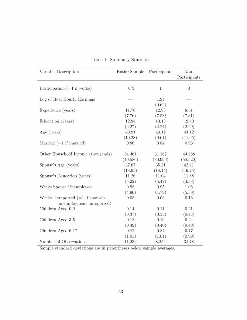
a participant if she reports positive work hours in a given year. Summary statistics for

the variables used in the analysis are presented in Table 1.

As discussed in the previous section, the semiparametric Procedure 5.3.1 will produce

consistent estimators of parameters in β1 only if exclusion restrictions are available. In

the considered application, the decision to work or not to work is likely to be affected by

spouse’s employment status in the current period. On the other hand, current employ-

ment status of the spouse should not affect woman’s current experience, since experience

is determined by past labor-leisure choices. This restriction validates the exclusion of

spouse’s weeks of unemployment and an indicator of whether this information was not

reported from the set of instruments used in the estimation of the primary equation. We

impose this exclusion restriction when using the semiparametric estimator.

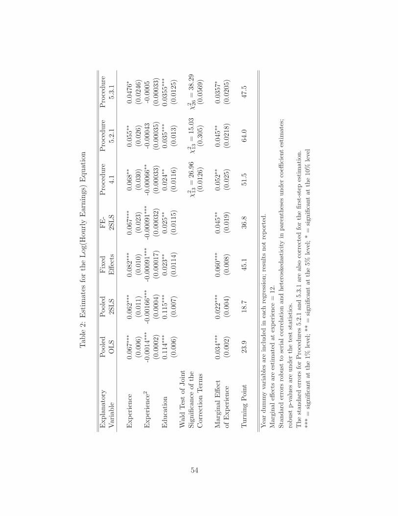
Table 2 reports the coefficient estimates from seven different estimation methods.

Pooled OLS assumes that all explanatory variables are uncorrelated with unobserved het-

erogeneity and are also strictly exogenous. Pooled 2SLS instruments for the experience

variables, but does not remove an unobserved effect. (So, for example, schooling is as-

sumed to be uncorrelated with unobserved ability and motivation.) Fixed effects allows

35

for correlation between the explanatory variables and unobserved heterogeneity while

FE-2SLS further allows experience (and its square, of course) to be correlated with the

idiosyncratic errors. Nevertheless, FE-2SLS assumes that selection into the workforce is

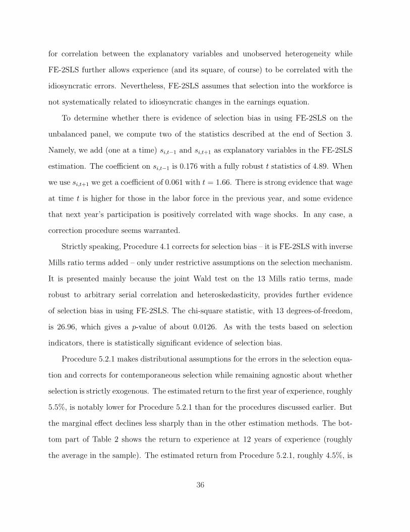
not systematically related to idiosyncratic changes in the earnings equation.

To determine whether there is evidence of selection bias in using FE-2SLS on the

unbalanced panel, we compute two of the statistics described at the end of Section 3.

Namely, we add (one at a time) si,t−1 and si,t+1 as explanatory variables in the FE-2SLS

estimation. The coefficient on si,t−1 is 0.176 with a fully robust t statistics of 4.89. When

we use si,t+1 we get a coefficient of 0.061 with t = 1.66. There is strong evidence that wage

at time t is higher for those in the labor force in the previous year, and some evidence

that next year’s participation is positively correlated with wage shocks. In any case, a

correction procedure seems warranted.

Strictly speaking, Procedure 4.1 corrects for selection bias – it is FE-2SLS with inverse

Mills ratio terms added – only under restrictive assumptions on the selection mechanism.

It is presented mainly because the joint Wald test on the 13 Mills ratio terms, made

robust to arbitrary serial correlation and heteroskedasticity, provides further evidence

of selection bias in using FE-2SLS. The chi-square statistic, with 13 degrees-of-freedom,

is 26.96, which gives a p-value of about 0.0126. As with the tests based on selection

indicators, there is statistically significant evidence of selection bias.

Procedure 5.2.1 makes distributional assumptions for the errors in the selection equa-

tion and corrects for contemporaneous selection while remaining agnostic about whether

selection is strictly exogenous. The estimated return to the first year of experience, roughly

5.5%, is notably lower for Procedure 5.2.1 than for the procedures discussed earlier. But

the marginal effect declines less sharply than in the other estimation methods. The bot-

tom part of Table 2 shows the return to experience at 12 years of experience (roughly

the average in the sample). The estimated return from Procedure 5.2.1, roughly 4.5%, is

36

equal to the estimate obtained from the FE-2SLS regression. However, the standard error

is somewhat larger once selection is accounted for. Procedure 5.2.1 also estimates a larger

turning point: the estimated return to experience becomes negative only after 64 years,

which far past the highest experience in the sample (roughly 45 years). Thus, according

to these estimates, the return to experience never becomes negative over the range of the

data and beyond that.

Not surprisingly, the years of schooling estimate is reduced dramatically by controlling

for an unobserved effect, but it is still statistically significant.

Before applying semiparametric estimation, we perform a series of specification tests

in the selection equation to find out whether the normality assumption may not hold.

In each time period, we estimate equation (21) by probit and use resulting estimates to

compute fitted values for the selection index. Then, the selection equation was augmented

by the second and third powers of the selection index and estimated by probit. We use the

standard Wald test to test the hypothesis that additional terms are jointly insignificant,

i.e. initial probit model is correct. The hypothesis was rejected at the 10% level in two

cases, at the 5% level – in two cases, and at the 1% level – in two cases, suggesting that

the parametric assumptions of Section 5.2 may be too strong.

When implementing the semiparametric approach of Section 5.3, we estimate the

selection equation by Ichimura’s (1993) estimator. Prior to estimation, a linear transfor-

mation was applied to the explanatory variables to obtain the sample covariance equal to

an identity matrix. The bandwidth was selected using the method proposed by Hardle,

Hall and Ichimura (1993), who suggest minimizing the mean squared error simultaneously

with respect to both parameters and the bandwidth. The search for the optimal band-

width was performed on the interval [0.1, 0.4] at 10 grid points. The kernel function was

chosen to be Gaussian. In the primary equation, we use the standard normal transforma-

tion of the selection index to construct the approximating functions. Linear and quadratic

37

terms, as well as their interactions with time dummies, were used to approximate ϕit.4

Estimates from the semiparametric correction procedure are reported in the last col-

umn of Table 2. Procedure 5.3 produces the coefficient estimate on the linear experience

term of about 4.8%, which is somewhat smaller than the estimate from Procedure 5.2.

In other words, the return to the first year of experience reduces further when we use

semiparametric correction. The marginal effect of experience evaluated at 12 years is

also smaller (only 3.6%). Due to lower estimated returns, Procedure 5.3.1 also gives a

smaller turning point (roughly 48 years), although it is still beyond the maximal years

of experience in the sample. In summary, correcting for endogeneity of experience and

sample selection results in flattening of the earnings-experience profile. Not surprisingly,

it also gives larger standard errors.

7 Simulations

In this section we present the results of limited Monte Carlo simulations that demonstrate

the properties of the test and estimators in finite samples. We consider a model described

by equations (6) and (8), where xit is a scalar, zit is a vector of two variables, and

β1 = δ21 = δ22 = 1. Unobserved effects, ci1 and ci2, are independent across i and

distributed as Normal(0, σ2c ). Idiosyncratic errors, uit1 and uit2, are independent across

i and t and distributed as Normal(0, σ2u). The total variance of the composite errors,

ci1 + uit1 and ci2 + uit2, is σ2 = σ2c + σ2

u = 1; the proportion of the total variance due

to the unobserved effect, σ2c/σ

2u, varies across experiments. The correlation between the

4We also tried including third and forth order polynomials of the transformed selection index and thecorresponding interactions with time dummies, but the higher power functions turned out to be highlycollinear with the linear and quadratic terms. Moreover, including more approximating functions hadlittle influence on the estimated coefficients of education, experience, and experience squared. Therefore,we chose to limit out attention to linear and quadratic terms.

38

unobserved effects is equal to 0.7, while ρu1,u2 ≡ Corr(uit1, uit2) varies depending on the

experiment.

The endogenous and exogenous variables were generated as follows:

zit1 = bi1 + εit1,

zit2 = bi2 + εit2,

xit = zit1 + ζuit1 + bi3 + εit3, (38)

where unobserved effects, bi1, bi2, and bi3, are independent across i and distributed as

Normal(0, σ2b ); idiosyncratic errors, εi1, εi2, and εi3, are independent across i and t and

distributed as Normal(0, σ2ε ). The total variance is σ2 = σ2

b + σ2ε = 1, and the proportion

of the total variance due to the corresponding unobserved effect changes from experiment

to experiment. The correlation between any two unobserved effects (including ci1 and ci2)

is equal to 0.7. Thus, all variables are correlated with each other through the unobserved

effects, whenever the unobserved heterogeneity is present. There is also a non-zero cor-

relation between xit and the idiosyncratic component of zit1. Coefficient ζ varies across

experiments. When performing simulations, we use zit = (zit1, zit2) as regressors in the

selection equation and use zit1 as an instrument for xit.

Table 3 presents Monte Carlo results for the size and power of the test described in

Section 4. Simulations were performed for N = 200 and 500, and T = 5 and 10, using

1000 replications. Because selection bias may arise due to unobserved heterogeneity, as

well as non-zero correlation between uit1 and uit2, the computed size of the test appears

on the intersection of the first column and the first row in each panel of the table. In all

experiments, the computed size of the test is close to the nominal size. The power of the

test increases with N and T , as well as when the correlation between the idiosyncratic

errors, ρu1,u2 , increases. However, when the proportion of the variance due to unobserved

39

heterogeneity rises, the power of the test is reduced because the share of σ2u falls.

When evaluating the performance of the estimators discussed in Section 5, we focus

on the following cases:

(i) σ2c = σ2

b = ζ = ρu1,u2 = 0. That is, there is no unobserved heterogeneity, xit is

strictly exogenous, and the idiosyncratic errors in the primary and selection equa-

tions are independent.

(ii) σ2c = σ2

b = 0.5, ζ = ρu1,u2 = 0. Here we introduce unobserved heterogeneity, but

maintain the assumption of zero correlation with idiosyncratic errors.

(iii) σ2c = σ2

b = ζ = 0.5, ρu1,u2 = 0. In addition to unobserved heterogeneity, we

introduce endogeneity of xit due to it being correlated with the idiosyncratic error

in the primary equation.

(iv) σ2c = σ2

b = ζ = ρu1,u2 = 0.5. In this case, we have all three components present:

unobserved heterogeneity, endogeneity, and selection due to correlation between the

idiosyncratic errors.

(v) σ2c = σ2

b = ζ = 0.5, ρu1,u2 = −0.5. This is almost like case (iv), but the idiosyncratic

errors in the selection and primary equation are negatively correlated.

We run simulations for N = 200 and T = 5. Number of replications is 1000. 5

Results are reported in Table 4. We computed the bias, average standard error and root

mean square error (RMSE) for six estimators: OLS, 2SLS, FE, FE-2SLS, the parametric

estimator discussed in Section 5.2, and the semiparametric estimator described in Section

5.3. Because in our simulations the number of regressors is equal to the number of

instruments, the 2SLS estimator is the same as the instrumental variables (IV) estimator.

5When using the semiparametric estimator described in Section 5.3, we estimate the selection equa-tion by Ichimura’s (1993) estimator. To reduce the computational burden, the bandwidth was fixed at(NT )−1/5.

40

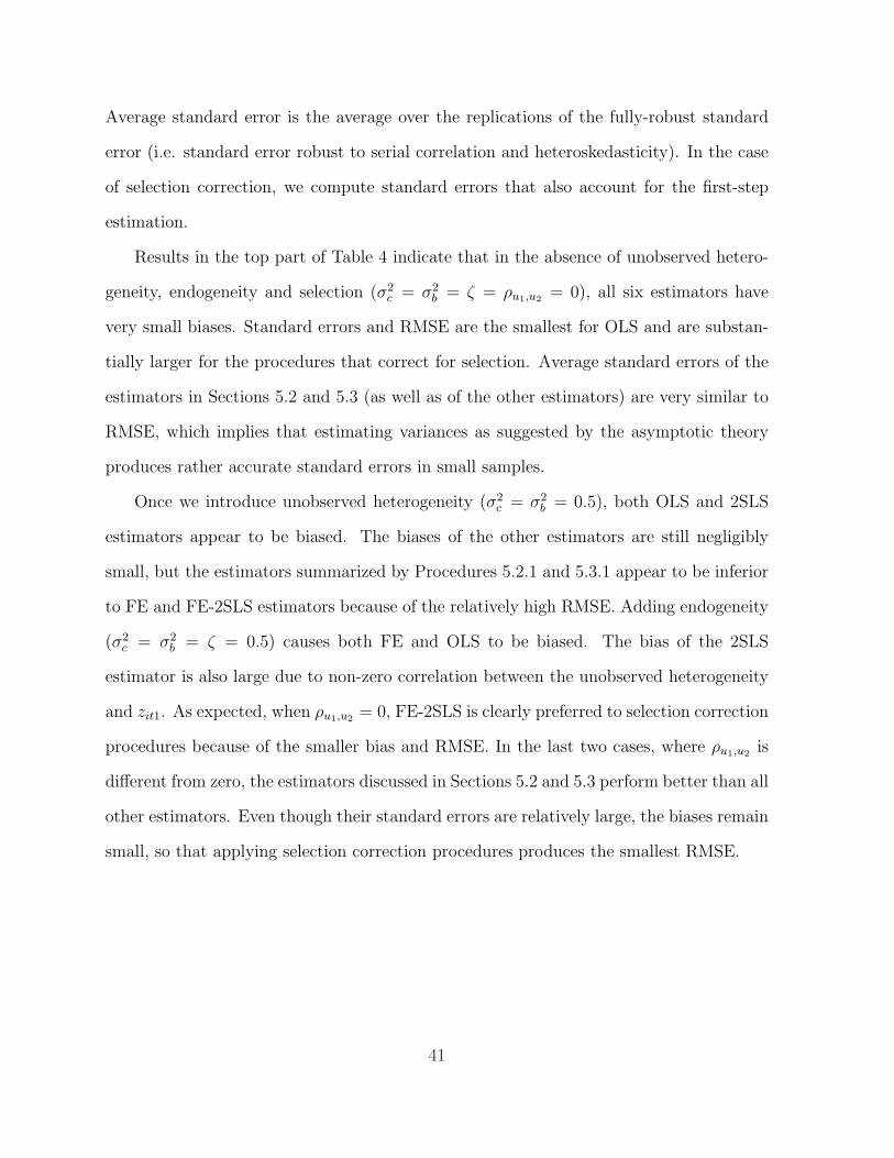
Average standard error is the average over the replications of the fully-robust standard

error (i.e. standard error robust to serial correlation and heteroskedasticity). In the case

of selection correction, we compute standard errors that also account for the first-step

estimation.

Results in the top part of Table 4 indicate that in the absence of unobserved hetero-

geneity, endogeneity and selection (σ2c = σ2

b = ζ = ρu1,u2 = 0), all six estimators have

very small biases. Standard errors and RMSE are the smallest for OLS and are substan-

tially larger for the procedures that correct for selection. Average standard errors of the

estimators in Sections 5.2 and 5.3 (as well as of the other estimators) are very similar to

RMSE, which implies that estimating variances as suggested by the asymptotic theory

produces rather accurate standard errors in small samples.

Once we introduce unobserved heterogeneity (σ2c = σ2

b = 0.5), both OLS and 2SLS

estimators appear to be biased. The biases of the other estimators are still negligibly

small, but the estimators summarized by Procedures 5.2.1 and 5.3.1 appear to be inferior

to FE and FE-2SLS estimators because of the relatively high RMSE. Adding endogeneity

(σ2c = σ2

b = ζ = 0.5) causes both FE and OLS to be biased. The bias of the 2SLS

estimator is also large due to non-zero correlation between the unobserved heterogeneity

and zit1. As expected, when ρu1,u2 = 0, FE-2SLS is clearly preferred to selection correction

procedures because of the smaller bias and RMSE. In the last two cases, where ρu1,u2 is

different from zero, the estimators discussed in Sections 5.2 and 5.3 perform better than all

other estimators. Even though their standard errors are relatively large, the biases remain

small, so that applying selection correction procedures produces the smallest RMSE.

41

8 Conclusion

We have shown how to estimate panel data models in the presence of selection when

the primary equation contains endogenous explanatory variables, where endogeneity is

conditional on the unobserved effect. These models arise in various economic applications,

such as estimation of earnings equations and labor supply models; therefore, the methods

discussed in this paper should provide a useful tool for applied economic research. The

proposed tests offer robust ways of testing for selection bias in the presence of endogenous

regressors. The suggested correction procedures provide an important alternative to some

existing methods, as they allow general serial correlation on idiosyncratic errors in the

primary and selection equations. Additionally, our semiparametric estimator shares the

properties of all semiparametric estimators in the sense that it is robust to a wide variety

of error distributions. The results of Monte Carlo simulations show that the estimators

perform reasonably well in small samples.

An avenue for further research is in relaxing the single-index assumption for the selec-

tion equation. Semiparametric and nonparametric procedures that relax the separability

of the unobserved effect from the effects of other variables in binary response panel data

models (see, for example, Altonji and Matzkin, 2005), can add to the flexibility of the

approach.

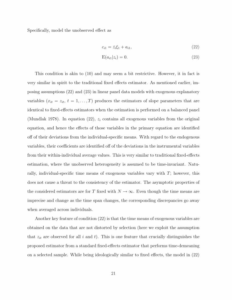
Appendix A

In this section, we present the derivation of the asymptotic variance of the estimators

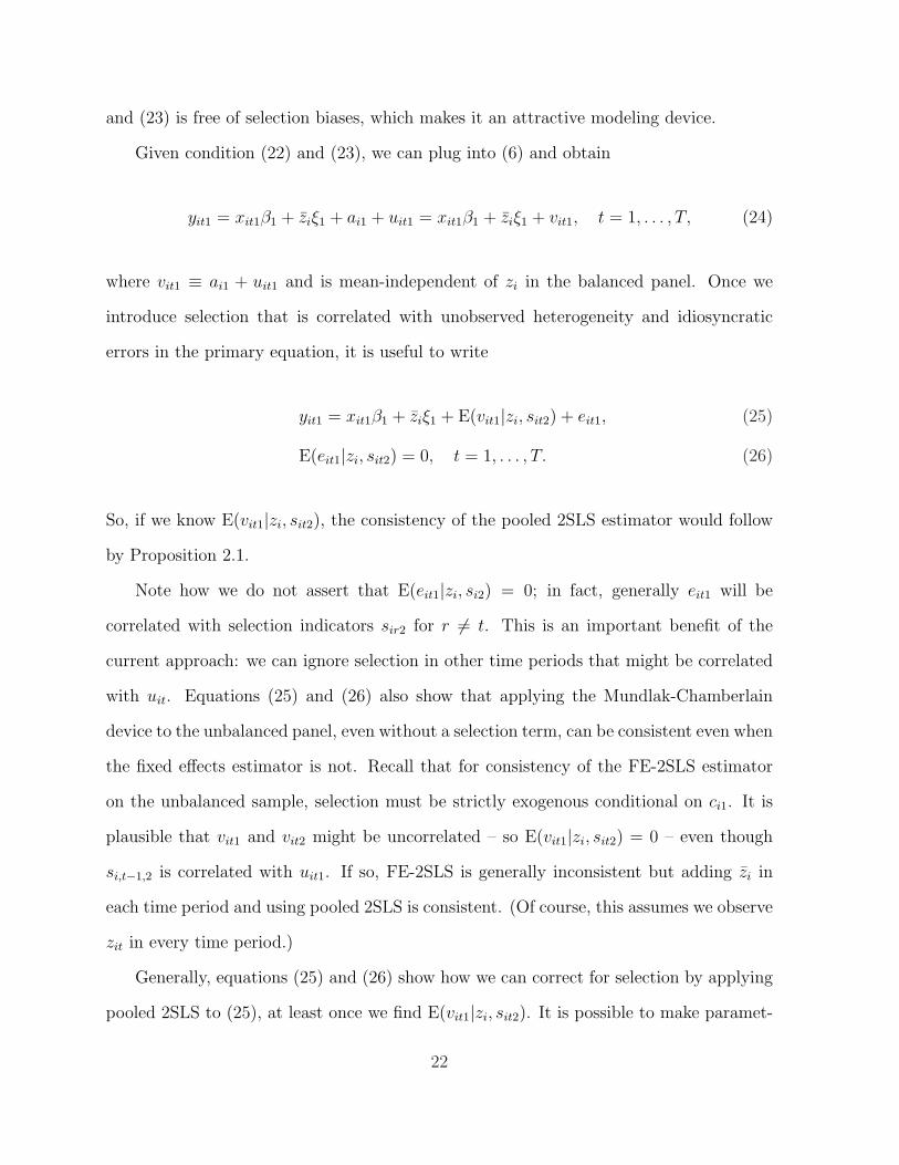
discussed in Procedures 5.2.1 and 5.3.1. Let either Assumption 5.2.1 hold so that yit1 can

be written as in (29), or let Assumption 5.3.1 hold and write yit1 as in (31). Technically,

we should use equation (25) with the parametric or semiparametric form of E(vit1|zi, sit2)

42

substituted in, but this expectation disappears for sit2 = 0, anyway. Therefore, we abuse

notation slightly and express yit1 as in (29) or (31) for the selected sample.

Define the generated regressors and instruments for time period t as wit = ( xit1,

zi, 0, . . ., 0, dit2, 0, . . ., 0) and hit = (zit1, zi, 0, . . ., 0, dit2, 0, . . ., 0), respectively,

where dit2 = λit2 (the inverse Mills ratio) if using Procedure 5.2.1, and dit2 = pit2 (the

set of approximating functions) if using Procedure 5.3.1. In the primary equation, the

parameter vector is θ = (β′1, ξ′1, γ

′11, . . . , γ

′T1)

′, where γt1 is a scalar when using parametric

correction, and it is an m × 1 vector when using series approximations. In the selection

equation, the parameter vectors are πt = (δ′t2, ξ′t2)

′, and π = (π′1, π′2, . . . , π

′T )′. When we

drop the “ˆ” over wit and hit, these are evaluated at the unknown population parameter,

π, rather than π.

The pooled 2SLS estimator on the selected sample, after plugging in the first-stage

estimates from the selection equations, is

θ =

(N∑

i=1

T∑t=1

sit2w′ithit

)(N∑

i=1

T∑t=1

sit2h′ithit

)−1 (N∑

i=1

T∑t=1

sit2h′itwit

)−1

×(

N∑i=1

T∑t=1

sit2w′ithit

)(N∑

i=1

T∑t=1

sit2h′ithit

)−1 (N∑

i=1

T∑t=1

sit2h′ityit1

); (39)

since yit1 = witθ + eit1 = witθ + (wit − wit)θ + eit1, we have upon substitution

43

√N(θ − θ) =

(N−1

N∑i=1

T∑t=1

sit2w′ithit

)(N−1

N∑i=1

T∑t=1

sit2h′ithit

)−1

×(

N−1

N∑i=1

T∑t=1

sit2h′itwit

)]−1

×(

N−1

N∑i=1

T∑t=1

sit2w′ithit

)(N−1

N∑i=1

T∑t=1

sit2h′ithit

)−1

×(

N−1/2

N∑i=1

T∑t=1

sit2h′it[(wit − wit)θ + eit1]

)

= (C ′D−1C)−1C ′D−1

×(

N−1/2

N∑i=1

T∑t=1

sit2h′it[(wit − wit)θ + eit1]

)+ op(1), (40)

where C ≡ E(∑T

t=1 sit2h′itwit

)and D ≡ E

(∑Tt=1 sit2h

′ithit

). [Naturally, the representa-

tion in (40) assumes regularity conditions, but we suppress those here.] Using an argument

similar to Wooldridge (2002, Chapter 6) and E(eit1|hit, sit2) = 0,

(N−1/2

N∑i=1

T∑t=1

sit2h′it[(wit − wit)θ + eit1]

)

= −E

[T∑

t=1

sit2h′it(θ

′∇πw′it)

]√N(π − π)

+N−1/2

N∑i=1

T∑t=1

sit2h′iteit1 + op(1), (41)

where ∇πw′it is the Jacobian of w′

it with respect to π. Because π is either a vector of

probit maximum likelihood estimators for each t, or a vector of semiparametric estimators

44

satisfying Assumption 5.3.4, we have

√N(π − π) = N−1/2

N∑i=1

ψi(π) + op(1), (42)

where ψi(π) depends on the expected Hessians and scores for either the probit log-

likelihoods or the first-step semiparametric estimators; more on this below. It follows

that

(N−1/2

N∑i=1

T∑t=1

sit2h′it[(wit − wit)θ + eit1]

)

= N−1/2

N∑i=1

[T∑

t=1

sit2h′iteit1 − Fψi(π)

]+ op(1), (43)

where F = E[∑T

t=1 sit2h′it(θ

′∇πw′it)

]. Combining (43) and (40) gives

√N(θ − θ)

= (C ′D−1C)−1C ′D−1

(N−1/2

N∑i=1

[T∑

t=1

sit2h′iteit1 − Fψi(π)

])

+op(1) (44)

and so√

N(θ − θ)a

˜Normal[0, (C ′D−1C)−1C ′D−1GD−1C(C ′D−1C)−1] (45)

where

G = Var

(T∑

t=1

sit2h′iteit1 − Fψi(π)

)≡ Var[gi(θ, π)].

Consistent estimation of Avar[√

N(θ − θ)] is straightforward by replacing unknown pa-

45

rameters with their consistent estimators. Consistent estimators of C, D, and G are

C ≡ N−1

N∑i=1

T∑t=1

sit2h′itwit (46)

D = N−1

N∑i=1

T∑t=1

sit2h′ithit (47)

G = N−1

N∑i=1

gig′i, (48)

respectively, where gi =∑T

t=1 sit2h′iteit1 − F ψi, eit1 = yit1 − witθ, and F =

N−1∑N

i=1

∑Tt=1 sit2h

′it(θ

′∇πw′it). Only F and ψi require some work to compute. For

F we need to obtain ∇πw′it. But, for each (i, t), ∇πw′

it is easily seen to be a block matrix

with all blocks zero except one. Namely, if we let qit ≡ (zit, zi), then

∇πw′it =

0 0 · · · 0

0 0 · · · 0

...... · · · ...

0 0 −qitµit2 0

0 0 0 0

...... · · · ...

0 0 · · · 0

(49)

where µit2 = λit2 · (qitπt + λit2) [the derivative of the inverse Mills ratio, see Wooldridge

2002, p. 522] if use Procedure 5.2.1, and µit2 = ∇qitπtp′it if use Procedure 5.3.1. Further,

θ′∇πw′it = (0, . . . , 0,−γt1qitλit2 · (qitπt + λit2), 0, . . . , 0, ) for the parametric correction, and

θ′∇πw′it = (0, . . . , 0,−qit

dpitγt1

d(qitπt), 0, . . . , 0, ) if correct for selection semiparametrically. So,

if use Procedure 5.2.1,

46

F = −N−1

N∑i=1

T∑t=1

[0, . . . , 0, sit2h

′itγt1qitλit2 · (qitπt + λit2), 0, . . . , 0

]. (50)

And, if use Procedure 5.3.1,

F = −N−1

N∑i=1

T∑t=1

[0, . . . , 0, sit2h

′itqit

dpitγt1

d(qitπt), 0, . . . , 0

]. (51)

The expressions for ψi, will depend on the first-step estimator used for obtaining the

parameter estimates in the selection equation. In the semiparametric case, the formulae

will be different depending on the choice of the first-step semiparametric estimator. In the

case of parametric correction summarized by Procedure 5.2.1, the formulae are known.

Specifically, from standard results for probit, for each i and t we have vectors

ψit = H−1t Φ(qitπt)[1− Φ(qitπt)]−1φ(qitπt)q

′it[sit2 − Φ(qitπt)], (52)

where

Ht ≡ N−1

N∑i=1

Φ(qitπt)[1− Φ(qitπt)]−1[φ(qitπt)]2q′itqit (53)

is the consistent estimator of minus the expected Hessian, and πt is the maximum like-

lihood estimator from probit of sit2 on qit, i = 1, ..., N . For each i, we stack the ψit to

obtain ψi, which are then used in equation (48).

Appendix B

In this section, we provide the proof of Proposition 5.3.1. This proof relies on the results

derived by Newey (1988).

47

Define vectors of variables as in Section 5.3. Specifically, let wit = (xit1, zi), hit =

(zit1, zi), qit = (zit, zi), θ = (β′1, ξ′1)′, and πt = (δ′t2, ξ

′t2)

′. Rewrite (34) to obtain

θ = θ

+

T∑t=1

N∑i=1

sit2(wit − mwit)′hit

(T∑

t=1

N∑i=1

sit2(hit − mhit)′hit

)−1 T∑t=1

N∑i=1

sit2(hit − mhit)′wit

−1

×T∑

t=1

N∑i=1

sit2(wit − mwit)′hit

(T∑

t=1

N∑i=1

sit2(hit − mhit)′hit

)−1

×T∑

t=1

N∑i=1

sit2(hit − mhit)′(ϕit + eit1), (54)

where ϕit ≡ ϕt(qitπt). Consider vector rit = (wit, hit) and define

mrt ≡ E(rit|qitπt, sit2 = 1),

mrit = pit

(N∑

i=1

sit2p′itpit

)−1 (N∑

i=1

sit2p′itrit

), t = 1, . . . , T. (55)

From parts (i)-(iv) of Assumption 5.3.3 and Assumptions 5.3.4 and 5.3.5, it follows

as in Newey (1988), proof of Theorem 1, that

N−1

N∑i=1

sit2(rit − mrit)′rit

p−→ E [sit2(rt −mrt )′(rt −mr

t )] , t = 1, . . . , T. (56)

48

Therefore,

N−1

N∑i=1

sit2(wit − mwit)′hit

p−→ E[sit2(wit −mw

t )′(hit −mht )

], t = 1, . . . , T,

N−1

N∑i=1

sit2(hit − mhit)′hit

p−→ E[sit2(hit −mh

t )′(hit −mh

t )], t = 1, . . . , T,

N−1

T∑t=1

N∑i=1

sit2(wit − mwit)′hit

p−→ A,

N−1

T∑t=1

N∑i=1

sit2(hit − mhit)′hit

p−→ B. (57)

Then, under Assumptions 5.3.2(i) and 5.3.2(ii), rearranging equation (54) will give

√N(θ − θ) = (AB−1A)−1AB−1 1√

N

T∑t=1

N∑i=1

sit2(hit − mhit)′(eit1 + ϕit) + op(1). (58)

Also, from parts (ii), (iv) and (v) of Assumption 5.3.3, Assumptions 5.3.4 and 5.3.5,

it follows as in Newey (1988), proof of Theorem 1, that for t = 1, . . . , T ,

1√N

N∑i=1

sit2(hit − mhit)′(eit1 + ϕit) =

1√N

N∑i=1

[sit2(hit −mh

t )′eit1 − Ftψit

]+ op(1),

where Ft = E[sit2(hit −mh

t )′ dϕit

d(qitπt)qit

]. Consequently,

1√N

T∑t=1

N∑i=1

sit2(hit − mhit)′(eit1 + ϕit)

=1√N

N∑i=1

[T∑

t=1

sit2(hit −mht )′eit1 −

T∑t=1

Ftψit

]+ op(1), (59)

So, by the central limit theorem,√

N(θ − θ)d−→ Normal(0, V ), where V is the

asymptotic variance of θ that can be consistently estimated using the estimator described

in Appendix A. The proof of consistency of V is available from the authors upon request.

49

References

Altonji, J.G. and Matzkin, R.L. 2005, Cross section and panel data estimators for non-

separable models with endogenous regressors. Econometrica 73, 1053-1102.

Askildsen, J.E., B.H. Baltagi and T.H. Holmas, 2003, Wage policy in the health care

sector: a panel data analysis of nurses’ labour supply, Health Economics 12, 705-719.

Chamberlain, G., 1980, Analysis with qualitative data, Review of Economic Studies 47,

225-238.

Charlier, E., B. Melenberg, and A. van Soest, 2001, An analysis of housing expenditure

using semiparametric models and panel data, Journal of Econometrics 101, 71-107.

Das, M., W.K. Newey, and F. Vella, 2003, Nonparametric estimation of sample selection

models. Review of Economic Studies 70, 33-58.

Donald, S.G. and W.K. Newey, 1994, Series estimation of semilinear models. Journal of

Multivariate Analysis 50, 30-40.

Dustmann, C. and M.E. Rochina-Barrachina, 2007, Selection correction in panel data

models: An application to the estimation of females’ wage equations. Econometrics

Journal 10, 263-293.

Hardle, W., P. Hall, and H. Ichimura, 1993, Optimal smoothing in single-index models.

Annals of Statistics 21, 157-178.

Ichimura, H., 1993, Semiparametric least squares (SLS) and weighted SLS estimation of

single-index models. Journal of Econometrics 58, 71120.

Gonzalez-Chapela, J., 2004, On the price of recreation goods as a determinant of female

labor supply. Unpublished manuscript.

50

Klein, R.L. and R.H. Spady, 1993, An efficient semiparametric estimator for binary

response models. Econometrica 61, 387421.

Kyriazidou, E., 1997, Estimation of a panel data sample selection model. Econometrica

65, 1335-1364.

Kyriazidou, E., 2001, Estimation of dynamic panel data sample selection models, Review

of Economic Studies 68, 543-572.

Lewbel, A., 2005, Simple endogenous binary choice and selection panel model estimators.

Unpublished manuscript, Boston College.

Mundlak, Y., 1978, On the pooling of time series and cross section data, Econometrica

46, 69-85.

Newey, W.K., 1988, Two step series estimation of sample selection models. Unpublished

manuscript, MIT (revised version January 1999).

Newey, W.K., 1994, The asymptotic variance of semiparametric estimators. Economet-

rica 62, 1349-1382.

Newey, W.K., 1997, Convergence rates and asymptotic normality for series estimators.

Journal of Econometrics 79, 147-168.

Powell, J.L., 1994, Estimation of semiparametric models, in: R.F. Engle and D. McFad-

den, (Eds.), Handbook of Econometrics, Vol. 4. North Holland, Amsterdam, pp.

2444-2521.

Robinson, P.M., 1988, Root-N-consistent semiparametric regression. Econometrica 56,

931-954.

Rochina-Barrachina, M.E., 1999, A new estimator for panel data sample selection mod-

els. Annales d’Economie et de Statistique 55/56, 153-181.

51

Rochina-Barrachina, M.E., 2000, New semiparametric pairwise difference estimators for

panel data sample selection models. The 5th chapter of the thesis dissertation

“Panel data sample selection models” at University College London (University of

London).

Vella, F. and M. Verbeek, 1999, Two-step estimation of panel data models with censored

endogenous variables and selection bias, Journal of Econometrics 90, 239-263.

Verbeek, M. and T. Nijman, 1992, Testing for selectivity bias in panel data models,

International Economic Review 33, 681-703.

Winder, K.L, 2004, Reconsidering the motherhood wage penalty. Unpublished manuscript.

Wooldridge, J.M., 1995, Selection corrections for panel data models under conditional

mean independence assumptions, Journal of Econometrics 68, 115-132.

Wooldridge, J.M., 2002, Econometric analysis of cross section and panel data. MIT

Press: Cambridge, MA.

52

Table 1: Summary Statistics

Variable Description Entire Sample Participants Non-Participants

Participation (=1 if works) 0.73 1 0

Log of Real Hourly Earnings — 1.94 —(0.62)

Experience (years) 11.76 12.93 8.51(7.76) (7.58) (7.31)

Education (years) 12.94 13.13 12.40(2.27) (2.24) (2.29)

Age (years) 40.91 40.12 43.12(10.28) (9.61) (11.65)

Married (=1 if married) 0.86 0.84 0.93

Other Household Income (thousands) 34.461 31.167 44.268(40.586) (30.996) (58.520)

Spouse’s Age (years) 37.07 35.21 42.21(18.05) (18.14) (16.75)

Spouse’s Education (years) 11.26 11.04 11.88(5.22) (5.47) (4.38)

Weeks Spouse Unemployed 0.98 0.95 1.06(4.96) (4.79) (5.39)

Weeks Unreported (=1 if spouse’s 0.08 0.06 0.16unemployment unreported)

Children Aged 0-2 0.14 0.11 0.21(0.37) (0.33) (0.45)

Children Aged 3-5 0.18 0.16 0.24(0.42) (0.40) (0.49)

Children Aged 6-17 0.82 0.84 0.77(1.01) (1.01) (0.99)

Number of Observations 11,232 8,254 3,978Sample standard deviations are in parentheses below sample averages.

53

Tab

le2:

Est

imat

esfo

rth

eLog

(Hou

rly

Ear

nin

gs)

Equat

ion

Exp

lana

tory

Poo

led

Poo

led

Fix

edFE

-P

roce

dure

Pro

cedu

reP

roce

dure

Var

iabl

eO

LS

2SLS

Effe

cts

2SLS

4.1

5.2.

15.

3.1

Exp

erie

nce

0.06

7∗∗∗

0.06

2∗∗∗

0.08

2∗∗∗

0.06

7∗∗∗

0.06

8∗∗

0.05

5∗∗

0.04

76∗

(0.0

06)

(0.0

11)

(0.0

10)

(0.0

23)

(0.0

30)

(0.0

26)

(0.0

246)

Exp

erie

nce2

-0.0

014∗∗∗

-0.0

0166∗∗∗

-0.0

0091∗∗∗

-0.0

0091∗∗∗

-0.0

0066∗∗

-0.0

0043

-0.0

005

(0.0

002)

(0.0

004)

(0.0

0017

)(0

.000

32)

(0.0

0033

)(0

.000

35)

(0.0

0033

)E

duca

tion

0.11

4∗∗∗

0.11

5∗∗∗

0.02

3∗∗

0.02

5∗∗

0.02

4∗∗

0.03

5∗∗∗

0.03

55∗∗∗

(0.0

06)

(0.0

07)

(0.0

114)

(0.0

115)

(0.0

116)

(0.0

13)

(0.0

125)

Wal

dTes

tof

Join

tSi

gnifi

canc

eof

the

χ2 13

=26

.96

χ2 13

=15

.03

χ2 26

=38

.29

Cor

rect

ion

Ter

ms

(0.0

126)

(0.3

05)

(0.0

569)

Mar

gina

lE

ffect

0.03

4∗∗∗

0.02

2∗∗∗

0.06

0∗∗∗

0.04

5∗∗

0.05

2∗∗

0.04

5∗∗

0.03

57∗

ofE

xper

ienc

e(0

.002

)(0

.004

)(0

.008

)(0

.019

)(0

.025

)(0

.021

8)(0

.020

5)

Tur

ning

Poi

nt23

.918

.745

.136

.851

.564

.047

.5

Yea

rdu

mm

yva

riab

les

are

incl

uded

inea

chre

gres

sion

;re

sult

sno

tre

port

ed.

Mar

gina

leff

ects

are

esti

mat

edat

expe

rien

ce=

12.

Stan

dard

erro

rsro

bust

tose

rial

corr

elat

ion

and

hete

rosk

edas

tici

tyin

pare

nthe

ses

unde

rco

effici

ent

esti

mat

es;

robu

stp-

valu

esar

eun

der

the

test

stat

isti

cs.

The

stan

dard

erro

rsfo

rP

roce

dure

s5.

2.1

and

5.3.

1ar

eal

soco

rrec

ted

for

the

first

-ste

pes

tim

atio

n.**

*=

sign

ifica

ntat

the

1%le

vel;

**=

sign

ifica

ntat

the

5%le

vel;

*=

sign

ifica

ntat

the

10%

leve

l

54

Table 3: Computed Size and Power of the Test (Procedure 4.1), σ2 = 1, ζ = 0.5

ρu1,u2 σ2c = σ2

b =0 σ2c = σ2

b =0.3 σ2c = σ2

b =0.5 σ2c = σ2

b =0.7

N = 200, T = 5

0.0 0.052 0.060 0.056 0.0460.1 0.120 0.082 0.081 0.0660.2 0.244 0.187 0.147 0.1250.3 0.501 0.340 0.260 0.1760.4 0.750 0.568 0.408 0.2660.5 0.904 0.750 0.579 0.419

N = 200, T = 10

0.0 0.053 0.040 0.063 0.0390.1 0.181 0.134 0.126 0.0940.2 0.556 0.369 0.292 0.1950.3 0.866 0.707 0.567 0.3690.4 0.986 0.901 0.822 0.5950.5 1.000 0.989 0.946 0.793

N = 500, T = 5

0.0 0.048 0.065 0.050 0.0550.1 0.154 0.126 0.099 0.1040.2 0.539 0.359 0.277 0.1900.3 0.885 0.672 0.552 0.3920.4 0.984 0.904 0.762 0.5730.5 1.000 0.978 0.924 0.772

N = 500, T = 10

0.0 0.045 0.054 0.039 0.0460.1 0.386 0.261 0.216 0.1530.2 0.902 0.753 0.604 0.4230.3 0.999 0.983 0.915 0.7570.4 1.000 1.000 0.992 0.9480.5 1.000 1.000 1.000 0.996The table displays the fraction of rejections of the null hypothesis thatρ1 = 0 (see equation 19) out of 1000 replications.The nominal size of the test is 0.05.

55

Table 4: Performance of Parametric and Semiparametric Estimators, σ2 = 1, N = 200,T = 5

OLS 2SLS FE FE-2SLS Procedure 5.2.1 Procedure 5.3.1

σ2c = σ2

b = ζ = ρu1,u2 = 0

Bias -0.0005 0.0004 0.0008 0.0021 -0.0014 0.0041Average std. err. 0.0335 0.0507 0.0427 0.0649 0.0671 0.0683RMSE 0.0326 0.0499 0.0424 0.0628 0.0686 0.0679

σ2c = σ2

b = 0.5, ζ = ρu1,u2 = 0

Bias 0.1928 0.1657 -0.0009 -0.0008 -0.0015 0.0015Average std. err. 0.0369 0.0488 0.0389 0.0567 0.0636 0.0669RMSE 0.1964 0.1729 0.0395 0.0546 0.0626 0.0672

σ2c = σ2

b = ζ = 0.5, ρu1,u2 = 0

Bias 0.3336 0.1608 0.2628 -0.0034 -0.0056 -0.0002Average std. err. 0.0331 0.0474 0.0363 0.0571 0.0643 0.0669RMSE 0.3354 0.1679 0.2654 0.0577 0.0648 0.0672

σ2c = σ2

b = ζ = ρu1,u2 = 0.5

Bias 0.2903 0.0965 0.2359 -0.0686 -0.0026 -0.0042Average std. err. 0.0338 0.0503 0.0368 0.0604 0.0630 0.0664RMSE 0.2924 0.1096 0.2389 0.0912 0.0635 0.0686

σ2c = σ2

b = ζ = 0.5, ρu1,u2 = −0.5

Bias 0.3734 0.2252 0.2810 0.0601 -0.0010 0.0039Average std. err. 0.0326 0.0453 0.0347 0.0529 0.0639 0.0660RMSE 0.3749 0.2299 0.2831 0.0823 0.0668 0.0671

Monte Carlo results are obtained using 1000 replications.Averaged standard errors are robust to serial correlation and heteroskedasticity.Standard errors for Procedures 5.2.1 and 5.3.1 are also corrected for the first-step estimation.

56