1 Estimating Summertime Evapotranspiration Across Indiana Principal Investigators: Johnny Nykiel Undergraduate Department of Earth and Atmospheric Science Ryan Knutson Undergraduate Department of Earth and Atmospheric Science Jesse Steinweg-Woods Ph.D. student Texas A&M University Department of Atmospheric Science Ken Scheeringa Associate State Climatologist Dr. Dev Niyogi Associate Professor of Agronomy and Earth & Atmospheric Sciences and Indiana State Climatologist First Submission: July 2011 Second Submission: July 2012
Transcript
1
Estimating Summertime Evapotranspiration Across Indiana
Principal Investigators:
Johnny Nykiel
Undergraduate Department of Earth and Atmospheric Science
Ryan Knutson
Undergraduate Department of Earth and Atmospheric Science
Jesse Steinweg-Woods
Ph.D. student Texas A&M University Department of Atmospheric Science
Ken Scheeringa
Associate State Climatologist
Dr. Dev Niyogi Associate Professor of Agronomy and Earth & Atmospheric Sciences
and Indiana State Climatologist
First Submission: July 2011
Second Submission: July 2012
2
Abstract
Evapotranspiration (ET) describes the sum of plant transpiration and evaporation into the
atmosphere from soils. This is a critical component of the regional water cycle. Yet historical
measurements of ET do not exist in Indiana. Therefore, models are needed to develop ET
estimates. It is anticipated that using these models with verification from limited ET
measurements, the development of an Indiana ET climatology can be completed.
ET gages were installed at two Purdue Agricultural Centers (PAC) in the 2008 growing
season and nine PAC locations in the 2009 and 2010 growing seasons over a grass “reference”
vegetative surface. Comparisons were made between these reference ET (RefET) measurements
and several RefET models. The model weather inputs included temperature, solar radiation,
wind, and dew point temperature. Solar radiation serves as a proxy for net radiation which is not
measured at the PAC. The comparisons were divided into two categories. The first compared
RefET measurements with the simulation models when all measured weather inputs were taken
at the PAC sites. The second category of comparisons focused on model weather inputs
observed at nearby airports. These locations were determined by the proximity of the airport to
the RefET gage location at the PAC. Six airport locations were used in this study. The airports
and the paired RefET gage PAC include Valparaiso (PPAC), Evansville (SWPAC), Lafayette
(ACRE and TPAC), Cincinnati (SEPAC), Fort Wayne (NEPAC), and Muncie (DPAC).
A correlation analysis was undertaken comparing the measured and modeled RefET. In
both study categories, 11 separate models were run to calculate RefET to compare with the
RefET gage measurements. The results suggest the FAO 56 Penman-Monteith and Full ASCE
Penman-Monteith model performed best compared to the measurements. Depending on crop
type, the typical RefET rates for a growing season across Indiana are approximately 75 mm per
month or about 45 mm of crop ET loss per month.
Keywords: ET, Evapotranspiration, evaporation, transpiration, water cycle, RefET
3
1. Introduction
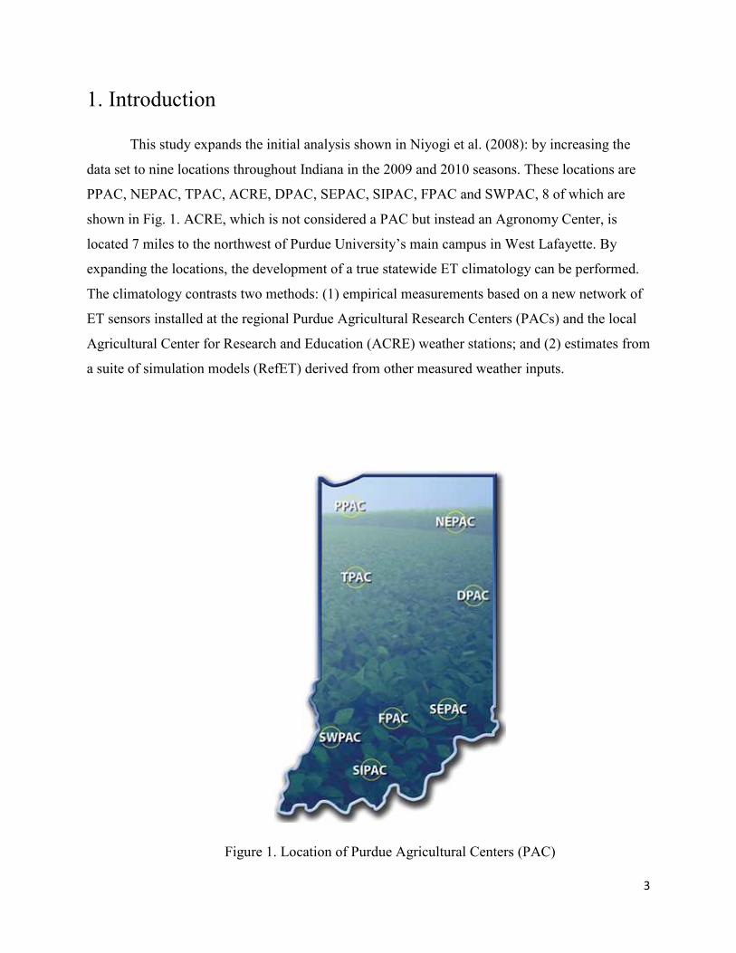
This study expands the initial analysis shown in Niyogi et al. (2008): by increasing the
data set to nine locations throughout Indiana in the 2009 and 2010 seasons. These locations are
PPAC, NEPAC, TPAC, ACRE, DPAC, SEPAC, SIPAC, FPAC and SWPAC, 8 of which are
shown in Fig. 1. ACRE, which is not considered a PAC but instead an Agronomy Center, is
located 7 miles to the northwest of Purdue University’s main campus in West Lafayette. By
expanding the locations, the development of a true statewide ET climatology can be performed.
The climatology contrasts two methods: (1) empirical measurements based on a new network of
ET sensors installed at the regional Purdue Agricultural Research Centers (PACs) and the local
Agricultural Center for Research and Education (ACRE) weather stations; and (2) estimates from
a suite of simulation models (RefET) derived from other measured weather inputs.
Figure 1. Location of Purdue Agricultural Centers (PAC)
4
1.1. What is Reference Evapotranspiration?
Evaporation is a form of vaporization in which a liquid is converted into a gas or vapor.
On the other hand, transpiration is the process in which there is a loss of water vapor from the
plant’s stomata. Often these occur together in nature and are referred to as evapotranspiration
(ET), that is, it includes both the evaporation and transpiration components. The rate of ET is
highly regulated by plant and growth stage. To allow general application to many crop types, ET
measurements are referenced to a standard crop, either grass or alfalfa. According to Niyogi et al
(2008), international criteria have been set to define what a standard crop of grass and alfalfa are.
The standard crop is an extensive surface of clipped grass or alfalfa that is well-watered and fully
shades the ground. The clipped grass reference should be a cool-season variety such as perennial
fescue or rye grass. Alfalfa that is greater than 30 cm in height and has full ground cover
complies with the reference standard. In common usage the suggested height of the standard
alfalfa crop is fixed at 50 cm.
The term RefET (Reference ET) is defined as ET measurements for these standard crops.
According to Niyogi et al (2008), “in order to apply RefET results to all other non-standard
crops, multiplier crop coefficients (K) have been developed to convert the reference data to each
alternate crop and growth stage. Two sets of coefficients are available for each non-standard
crop: one for conversion from a grass reference crop and the second set for an alfalfa reference
crop. Only one of these sets of K is necessary depending on which standard crop exists in the
immediate areas of the atmometer installation.”
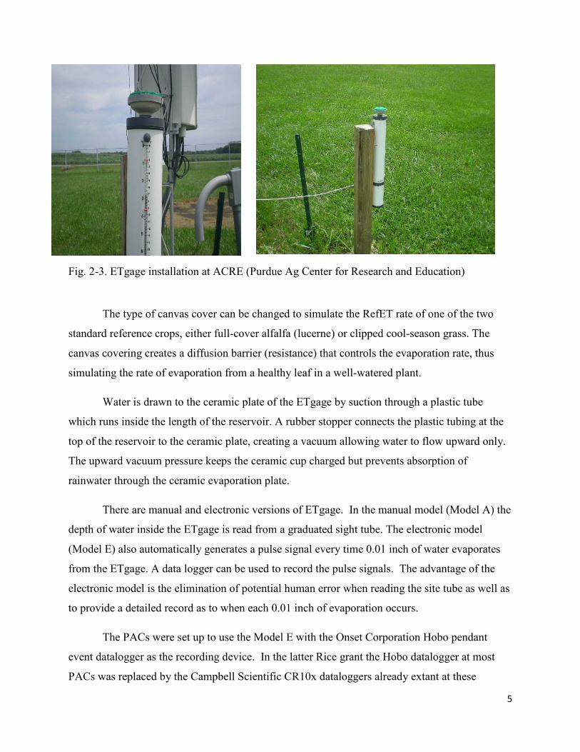
2. Materials and Methods An atmometer was used in this study to directly measure RefET. The gage used was the
modified Bellani Plate type, manufactured by ET Gage Company of Loveland, Colorado. Figure
2 and 3 show the ETgage with its ceramic plate mounted on top of the distilled water reservoir.
The reservoir capacity is 11.8 inches in depth. A green canvas (Gore-Tex) material covers the
ceramic plate. This canvas fabric mimics the absorption of incoming solar radiation and outgoing
water loss as if it were the crop canopy.
5
Fig. 2-3. ETgage installation at ACRE (Purdue Ag Center for Research and Education)
The type of canvas cover can be changed to simulate the RefET rate of one of the two
standard reference crops, either full-cover alfalfa (lucerne) or clipped cool-season grass. The
canvas covering creates a diffusion barrier (resistance) that controls the evaporation rate, thus
simulating the rate of evaporation from a healthy leaf in a well-watered plant.
Water is drawn to the ceramic plate of the ETgage by suction through a plastic tube
which runs inside the length of the reservoir. A rubber stopper connects the plastic tubing at the
top of the reservoir to the ceramic plate, creating a vacuum allowing water to flow upward only.
The upward vacuum pressure keeps the ceramic cup charged but prevents absorption of
rainwater through the ceramic evaporation plate.
There are manual and electronic versions of ETgage. In the manual model (Model A) the
depth of water inside the ETgage is read from a graduated sight tube. The electronic model
(Model E) also automatically generates a pulse signal every time 0.01 inch of water evaporates
from the ETgage. A data logger can be used to record the pulse signals. The advantage of the
electronic model is the elimination of potential human error when reading the site tube as well as
to provide a detailed record as to when each 0.01 inch of evaporation occurs.
The PACs were set up to use the Model E with the Onset Corporation Hobo pendant
event datalogger as the recording device. In the latter Rice grant the Hobo datalogger at most
PACs was replaced by the Campbell Scientific CR10x dataloggers already extant at these
6
automated weather stations.
In 2007 a first local installation permitted us to become familiar with the operation of the
ETgage and data collection by Onset Corporation Hobo Pendant data loggers. These loggers
only store point data when an ET event occurs, that is, a pulse signal that another .01 inch of ET
has evaporated. As these events are random points in time, the data were assigned to the
corresponding 30 minute time slot during the day in which the event occurred. This was done
for compatibility with the CR10x loggers which would replace most of the Hobo loggers in
2009.
The ETgage was easy to install and required little maintenance. It was mounted on a
wooden post 39 inches (one meter) above the ground, located over grass at a site representative
of the immediate area. The PAC ETgages were installed 3 to 7 feet away from the automated
weather station towers, enabling convenient connection to the data loggers. The ETgage ceramic
plate should not be shaded, which could reduce the RefET rate. Nor should it be installed near
tall trees, buildings, or tall crops that may prevent full exposure of the gauge to prevailing winds
and other environmental factors affecting RefET. The installations at the PAC automated
weather stations were in compliance with these requirements.
The ETgage reservoir was filled with distilled water. This prevents accumulation of salts
in the ceramic plate that could reduce its porosity and affect the evaporation rate. The ETgage
cannot be exposed to freezing temperatures and the canvas cover should be kept as clean as
possible. Bird spikes came with the ETgage to discourage birds from perching on the plate.
Two more installations were added in 2008, one at NEPAC and a second at ACRE.
These installations are co-located with official NWS cooperative weather stations. The ACRE
site is also equipped with a Class A evaporation pan. Again the PACs were set up to use the
ETgage Model E with the Hobo data logger as the recording device.
ET gages were installed at nine Purdue Agricultural Centers (PAC) in the 2009 and 2010
growing seasons to extend the data record and expand the RefET network statewide.. At this
time the Hobo data logger at most PACs were replaced by the Campbell Scientific CR10x data
loggers at these automated weather stations.
7
Estimation of ET for specific crops ((ETc) is calculated by multiplying RefET by the appropriate
crop coefficient Kc:
ETc = ETr x Kc
where ETr is the evapotranspiration (ET) of the reference crop (grass or alfalfa), expressed in
units of water depth per unit time (inches per day, week, etc).
3. Measurements vs. Models 3.1. Measurements
The Hobo pendant logger is designed to record an event and the timestamp at which the
event occurred. An event in our application occurs when the ETgage sends an electronic pulse to
the Hobo logger as each new 0.01 inch of ET evaporates from the canvas cover of the ETgage.
In our case it is easier to analyze the data in uniform time intervals rather than as random events.
With the expectation that in future years the Hobo logger would be replaced with a higher order
data logger, the format change to uniform time intervals made sense.
Our first data task then was to reformat the Hobo data into uniform hourly data intervals.
Software was written to do this conversion by assigning each event to the corresponding hourly
time bin. This was done for each ETgage location where the Hobo data logger was installed.
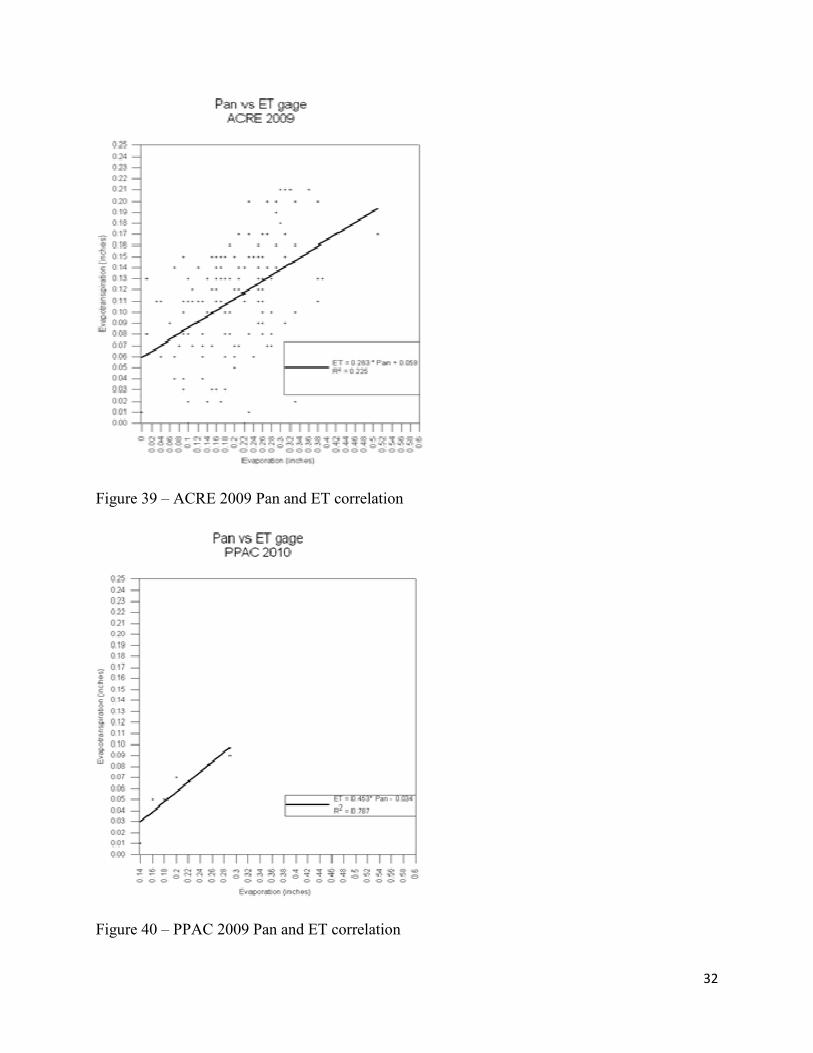
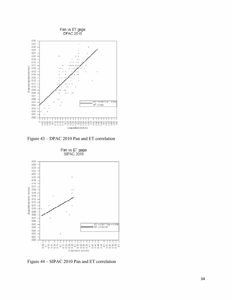
The ETgage data were summed by calendar day. The hourly and daily ETgage values
were then entered into an Excel spreadsheet. A column was added to the daily table to include
evaporation pan measurements where available.
Unfortunately, the data for the two stations SIPAC and FPAC were frequently missing (in
some cases, over 50% of the time) due to reliability issues with the Hobo loggers that were used
exclusively at these two sites. Because of this, no conclusions could be drawn from these two
stations.
8
3.2. Models
The software title Ref-ET (University of Idaho) offers many calculation models for
estimating reference evapotranspiration using equations currently in practice throughout the
United States and Europe. Figure 4 displays the full list of these models.
Method Timesteps Type a) “full” ASCE Penman-Monteith with resistances by Allen et al, 1989 (M, D, or H)** ETo ETr b) “full” ASCE Penman-Monteith with user supplied surf. resistance (M, D, or H)* ETo ETr c) Standardized form of the ASCE Penman-Monteith by ASCE 2005 (M, D, or H)* ETo ETr d) 1982 Kimberly Penman (Wright, 1982; 1987; 1996) (M, D, or H)* ETo ETr e) FAO 56 Penman-Monteith (1998)1 with resistance for 0.12 m grass (M, D, or H)* ETo f) 1972 Kimberly Penman (fixed wind func.) (Wright & Jensen 1972) (M, D, or H)* ETr g) 1948 or 1963 Penman (Penman, 1948; 1963) (M, D, or H) ETo h) FAO-24 Corrected Penman (Doorenbos and Pruitt, 1975, 1977) (M or D) ETo i) FAO-PPP-17 Penman (Freres and Popov, 1979) (M or D) ETo j) CIMIS Penman (hourly only) with FAO-56 Rn and G=0 (H) ETo k) FAO-24 Radiation Method (Doorenbos and Pruitt, 1975, 1977) (M or D) ETo l) FAO-24 Blaney-Criddle (Doorenbos and Pruitt, 1975, 1977) (M or D) ETo m) FAO-24 Pan Evaporation Method (Doorenbos and Pruitt, 1977) (M or D) ETo n) 1985 Hargreaves Temperature Method (Hargreaves and Samani) (M or D) ETo o) Priestley-Taylor (1972) Radiation and Temperature Method (M or D)* ETo p) Makkink (1957) Radiation and Temperature Method (M or D)* ETo q) Turc (1961) Radiation and Temperature Method (M or D)* ETo Figure 4 – Full list of Calculation Models
In this study, these models were run and the results were compared to the empirical
measurements. Weather inputs used in these models are the hourly data available from the
Purdue automated weather stations. Since the data is run through the software as hourly data, the
models return hourly products. The hourly ET model outputs were then summed into a daily
RefET value for comparison to the actual ET measurements. Not all models were able to produce
data. In some cases, required parameters and other criteria were not available. As a result, only
9
10 models were run for the case 1 study and 11 models for the case 2 study. Details on each case
are described later. The following models did not provide results for either case:
• “full” ASCE Penman-Monteith with user supplied surface resistance
• FAO-24 Corrected Penman (Doorenbos and Pruitt)
• FAO-PPP-17 Penman (Freres and Popov)
• FAO-24 Radiation Method (Doorenbos and Pruitt)
• FAO-24 Blaney-Criddle (Doorenbos and Pruitt)
• FAO-24 Pan Evaporation Method (Doorenbos and Pruitt)
• 1985 Hargreaves Temperature Method
In addition the following model did not provide results in case 1:
• “full” ASCE Penman-Monteith with user supplied surface resistance
3.3. Model Advantages
Why is it important to understand and estimate ET through models?
1. ET plays a major role in the regional water cycle balance. During drought conditions,
evapotranspiration continues to deplete the remaining water supply in lakes, streams,
vegetation and soil.
2. ET measurements cannot be made on days with subfreezing temperatures; therefore,
models become the only method for estimating RefET. Although the RefET values
during such subfreezing days are quite low, cold season precipitation does play a major
role in the recharge phase of the water cycle.
3. Models are useful for filling in missing data when measurements become unavailable.
Given good correlation with measurements, models can estimate the results for these
missing data points.
10
3.4. Model Disadvantages
1. RefET models require measured weather inputs; therefore it is necessary to perform
quality assurance on this source data in order to trust model accuracy.
2. Some weather variables are not commonly measured and can be difficult to obtain, such
as solar radiation.
3. Automated weather station maintenance is necessary so they continue working properly
and the technology stays updated. Some common problems can include communication
failures, dead backup batteries, sensor malfunction, and improper refilling of the ETgage.
The installation of the ETgage does require time to install initially and refill in mid-
season.
4. Results
Some questions can now be assessed to determine which model performs best in
determining evapotranspiration under two scenarios or case studies. The first study compared
hourly RefET measurements to simulation models when all weather inputs were present at a
single PAC location. The second study compared measurements to models when model weather
inputs except solar radiation were made at nearby airports.
4.1. Case 1: Hourly RefET measurements and models at the same location.
Regression correlations can be run to compare the models to the observed ETgage data.
In doing so, this can quantify the strength of the relationship between the models and the actual
ETgage data. The correlation results for the years 2009 and 2010 for all locations are shown in
fig. 5-11.
11
Figure 5 – ACRE station correlation results
Figure 6 – NEPAC station correlation results
12
Figure 7 – DPAC station correlation results
Figure 8 – TPAC station correlation results
13
Figure 9 – SEPAC station correlation results
Figure 10 – SWPAC station correlation results
14
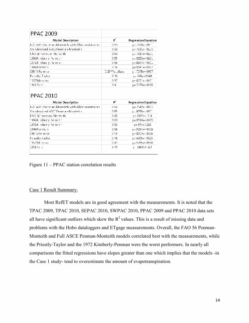
Figure 11 – PPAC station correlation results
Case 1 Result Summary:
Most RefET models are in good agreement with the measurements. It is noted that the
TPAC 2009, TPAC 2010, SEPAC 2010, SWPAC 2010, PPAC 2009 and PPAC 2010 data sets
all have significant outliers which skew the R2 values. This is a result of missing data and
problems with the Hobo dataloggers and ETgage measurements. Overall, the FAO 56 Penman-
Monteith and Full ASCE Penman-Monteith models correlated best with the measurements, while
the Priestly-Taylor and the 1972 Kimberly-Penman were the worst performers. In nearly all
comparisons the fitted regressions have slopes greater than one which implies that the models -in
the Case 1 study- tend to overestimate the amount of evapotranspiration.
15
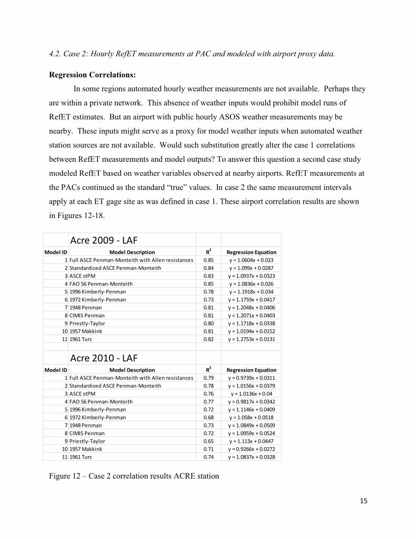
4.2. Case 2: Hourly RefET measurements at PAC and modeled with airport proxy data.
Regression Correlations:
In some regions automated hourly weather measurements are not available. Perhaps they
are within a private network. This absence of weather inputs would prohibit model runs of
RefET estimates. But an airport with public hourly ASOS weather measurements may be
nearby. These inputs might serve as a proxy for model weather inputs when automated weather
station sources are not available. Would such substitution greatly alter the case 1 correlations
between RefET measurements and model outputs? To answer this question a second case study
modeled RefET based on weather variables observed at nearby airports. RefET measurements at
the PACs continued as the standard “true” values. In case 2 the same measurement intervals
apply at each ET gage site as was defined in case 1. These airport correlation results are shown
in Figures 12-18.
Figure 12 – Case 2 correlation results ACRE station
Acre 2009 - LAFModel ID Model Description R2 Regression Equation
1 Full ASCE Penman-Monteith with Allen resistances 0.85 y = 1.0604x + 0.0232 Standardized ASCE Penman-Monteith 0.84 y = 1.099x + 0.02873 ASCE stPM 0.83 y = 1.0937x + 0.03234 FAO 56 Penman-Monteith 0.85 y = 1.0836x + 0.0265 1996 Kimberly-Penman 0.78 y = 1.1918x + 0.0346 1972 Kimberly-Penman 0.73 y = 1.1759x + 0.04177 1948 Penman 0.81 y = 1.2048x + 0.04068 CIMIS Penman 0.81 y = 1.2071x + 0.04039 Priestly-Taylor 0.80 y = 1.1718x + 0.0338
10 1957 Makkink 0.81 y = 1.0194x + 0.015211 1961 Turc 0.82 y = 1.2753x + 0.0131
Acre 2010 - LAFModel ID Model Description R2 Regression Equation
1 Full ASCE Penman-Monteith with Allen resistances 0.79 y = 0.9739x + 0.03112 Standardized ASCE Penman-Monteith 0.78 y = 1.0156x + 0.03793 ASCE stPM 0.76 y = 1.0136x + 0.044 FAO 56 Penman-Monteith 0.77 y = 0.9817x + 0.03425 1996 Kimberly-Penman 0.72 y = 1.1146x + 0.04096 1972 Kimberly-Penman 0.68 y = 1.058x + 0.05187 1948 Penman 0.73 y = 1.0849x + 0.05098 CIMIS Penman 0.72 y = 1.0959x + 0.05249 Priestly-Taylor 0.65 y = 1.113x + 0.0447
10 1957 Makkink 0.71 y = 0.9266x + 0.027211 1961 Turc 0.74 y = 1.0837x + 0.0328
16
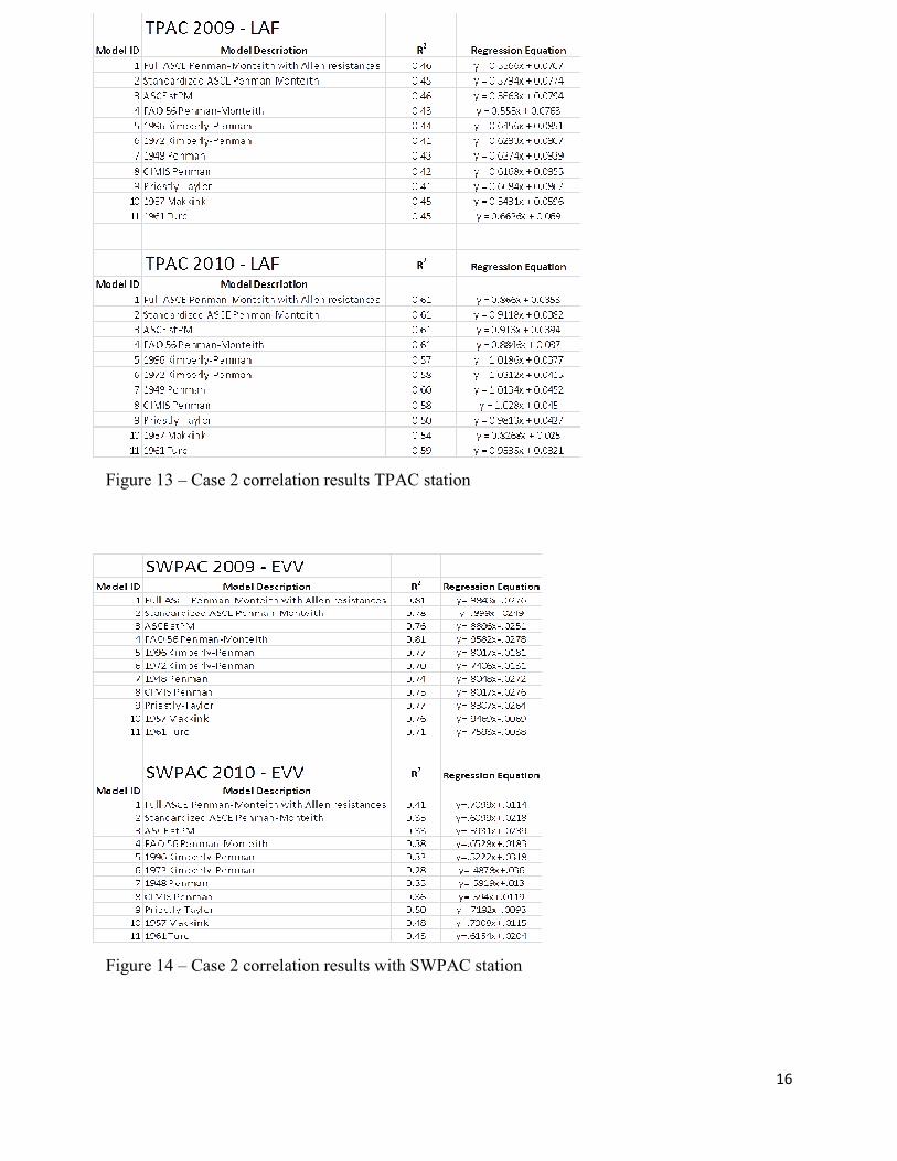
Figure 13 – Case 2 correlation results TPAC station
Figure 14 – Case 2 correlation results with SWPAC station
17
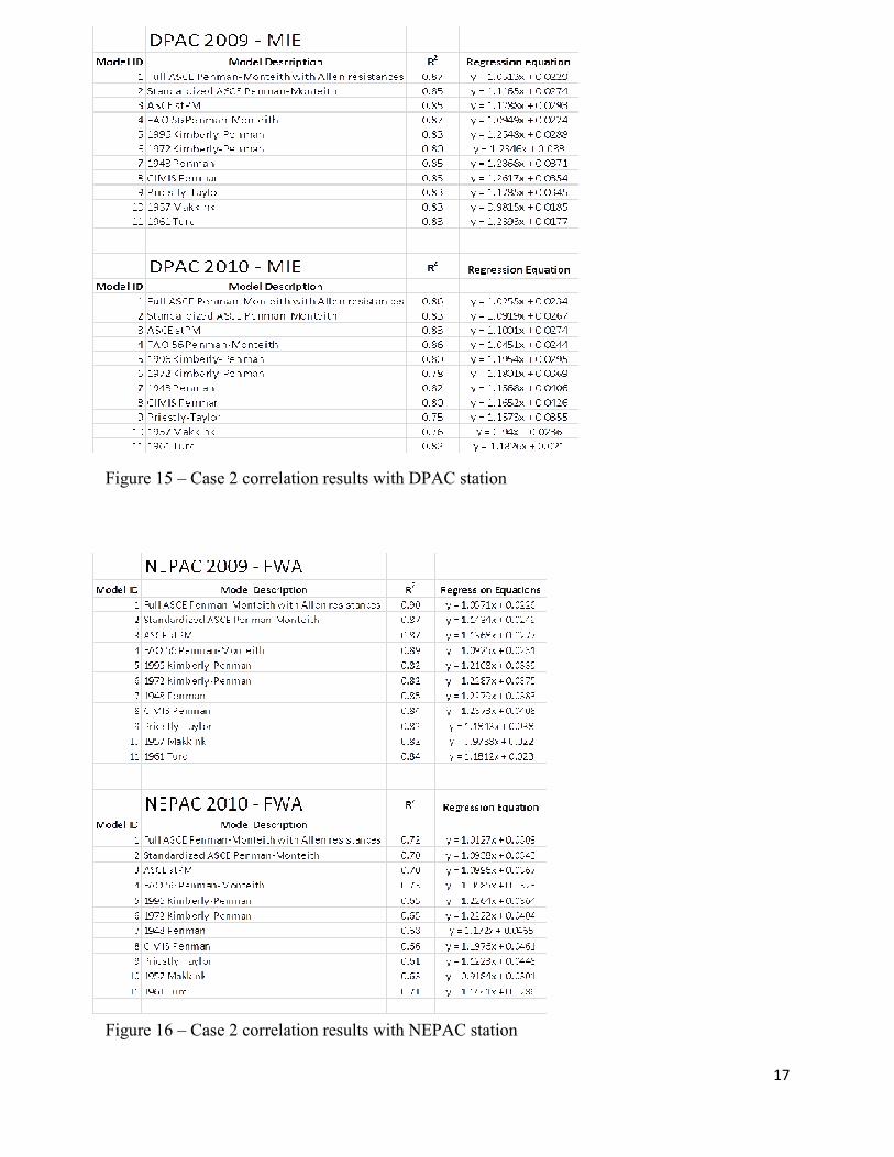
Figure 15 – Case 2 correlation results with DPAC station
Figure 16 – Case 2 correlation results with NEPAC station
18
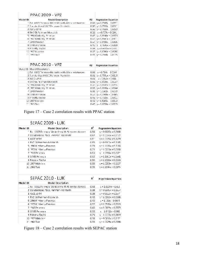
Figure 17 – Case 2 correlation results with PPAC station
Figure 18 – Case 2 correlation results with SEPAC station
19
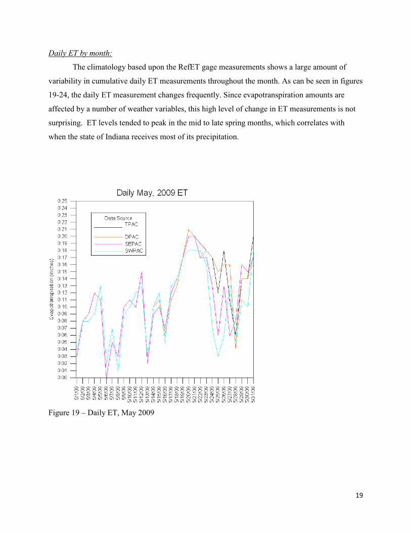
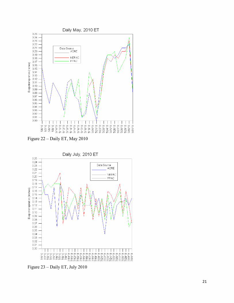
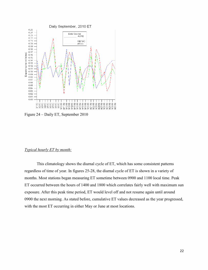
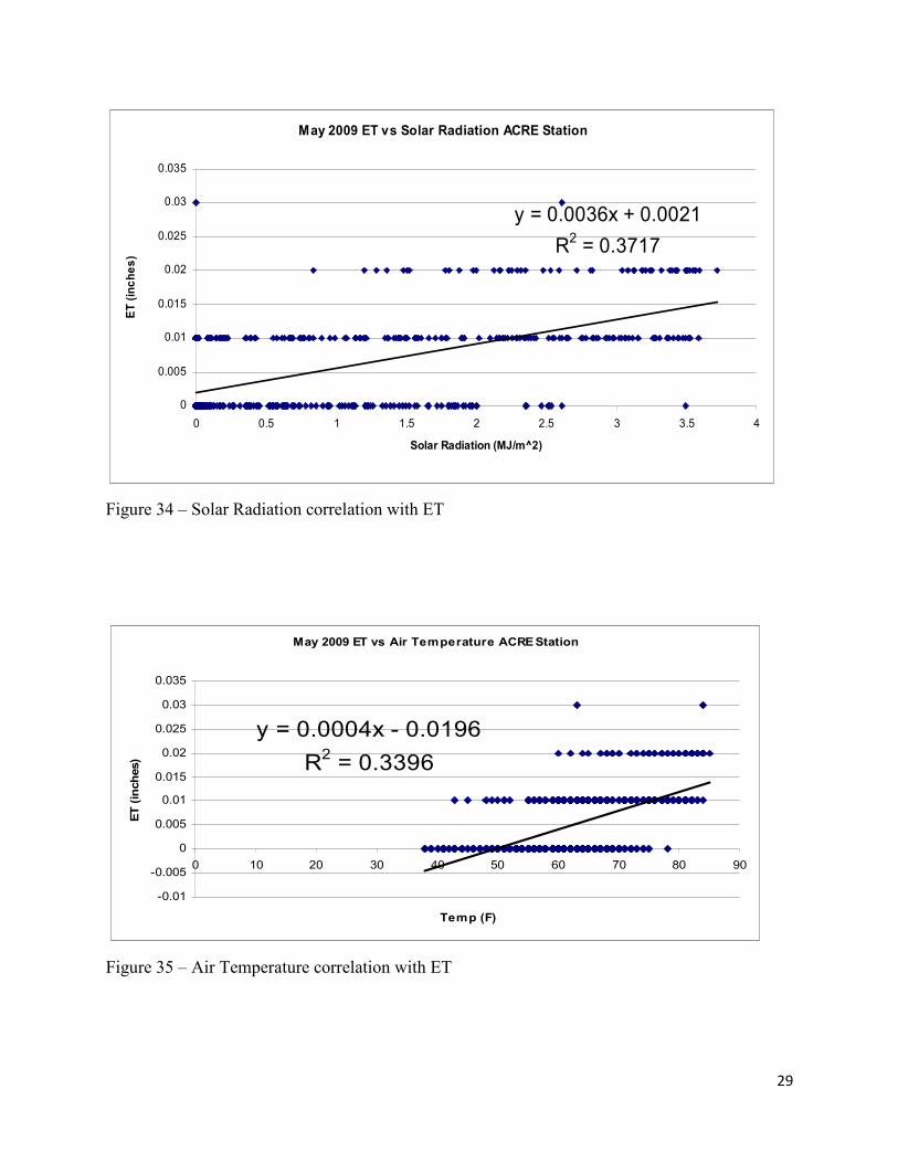
Daily ET by month:
The climatology based upon the RefET gage measurements shows a large amount of
variability in cumulative daily ET measurements throughout the month. As can be seen in figures
19-24, the daily ET measurement changes frequently. Since evapotranspiration amounts are
affected by a number of weather variables, this high level of change in ET measurements is not
surprising. ET levels tended to peak in the mid to late spring months, which correlates with
when the state of Indiana receives most of its precipitation.
Figure 19 – Daily ET, May 2009
20
Figure 20 – Daily ET, June 2009
Figure 21 – Daily ET, August 2009
21
Figure 22 – Daily ET, May 2010
Figure 23 – Daily ET, July 2010
22
Figure 24 – Daily ET, September 2010
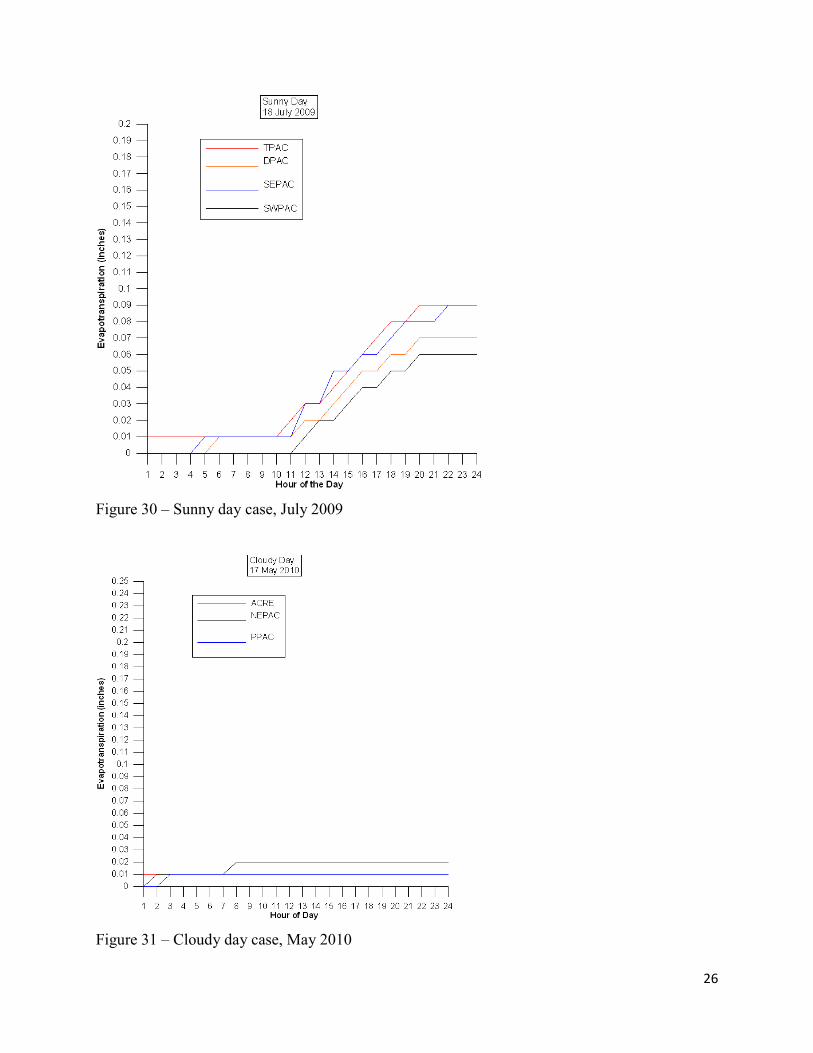
Typical hourly ET by month:
This climatology shows the diurnal cycle of ET, which has some consistent patterns
regardless of time of year. In figures 25-28, the diurnal cycle of ET is shown in a variety of
months. Most stations began measuring ET sometime between 0900 and 1100 local time. Peak
ET occurred between the hours of 1400 and 1800 which correlates fairly well with maximum sun
exposure. After this peak time period, ET would level off and not resume again until around
0900 the next morning. As stated before, cumulative ET values decreased as the year progressed,
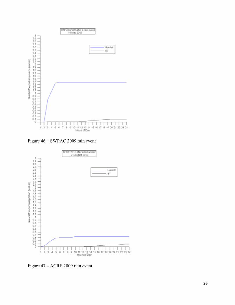
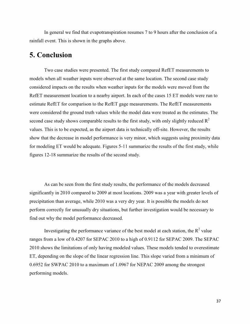
with the most ET occurring in either May or June at most locations.