Estimation of Lens Distortion Correction from Single Images

Miroslav Goljan and Jessica Fridrich

Department of ECE, SUNY Binghamton, NY, USA, {mgoljan,fridrich}@binghamton.edu

ABSTRACT

In this paper, we propose a method for estimation of camera lens distortion correction from a single image.Without relying on image EXIF, the method estimates the parameters of the correction by searching for amaximum energy of the so-called linear pattern introduced into the image during image acquisition prior tolens distortion correction. Potential applications of this technology include camera identification using sensorfingerprint, narrowing down the camera model, estimating the distance between the photographer and thesubject, forgery detection, and improving the reliability of image steganalysis (detection of hidden data).

1. MOTIVATION

Thanks to the increasing power of processors currently used in consumer digital cameras, manufacturers beganimplementing various computational imaging technology inside the camera to allow the photographer to takebetter images using cheaper hardware and optics. Most cameras today compensate for the imperfections of theoptical system by correcting for the geometrical lens distortion (LD) and chromatic aberration inside the camerabefore saving the resulting image to the memory card. Such processing leaves detectable traces that can beexploited for a variety of forensic purposes.

In this paper, we introduce a technique that can estimate the parameters of the lens distortion correctionfrom a single image. The method makes use of the so-called linear pattern (LP)1, 2 commonly present in digitalimages. It manifests through non-zero sums of rows and columns in the image noise residual. The LP is causedby several processes that are applied at different times in the image acquisition pipeline. The first component ofthe LP, L0, is due to sensor signal readout; this part is present in the raw sensor output. Another component, L1,is added during color interpolation (demosaicking) and JPEG compression. The part of the LP that is introducedbefore the LD correction is applied becomes deformed in the image corrected for the LD and thus can be usedas a template to estimate the parameters of the LD. The method proposed here estimates the parameters of theinverse LD correction transformation using the energy of the LP, particularly of the component L0.

We work under the assumption that a forensic analyst has one image under investigation (the test image)and, optionally, knows the model of the camera that took the image. In particular, we assume no knowledgeof the image EXIF header as this meta data can be replaced or lost when editing the image. Additionally, weassume that the image was not off-center cropped, rotated, or corrected for perspective distortion.∗ The analystdesires to estimate the amount of LD correction that was applied to the test image. There are numerous potentialapplications of such an estimation method:

1. It can be used as a front-end for camera identification using sensor fingerprints.2 Sensor fingerprints mustbe resynchronized with the noise residual of the test image prior to applying a correlation-based detector.4

The proposed technique can be used to resynchronize the residual with the fingerprint, thus saving onprocessing time when a large number of fingerprints need to be checked.

2. By detecting the presence or absence of camera LD correction, one could potentially narrow down themodel of the camera that took the test image, e.g., eliminate cameras whose optical system cannot notintroduce distortion of a certain strength.

∗The method could be potentially extended to these cases at the expense of increased computational complexity andlowered accuracy.

3. When the camera model is known, the estimated parameters could be used to determine the focal length(zoom) at which the image was taken. This could be further used to estimate the proximity of thephotographer to the object.

4. The image resampling due to LD correction introduces a specific global structure of pixel correlations intothe image† that might be locally disturbed when an object in the image (region of interest) is replaced,deleted, or manipulated. This may be useful for forgery detection.7

5. The symmetry of the deformed LP can also be used to determine the optical center of the image and thusdetect off-center image cropping. This would require an appropriate extension of the LD model used inthis paper.

6. It has been established that the reliability of steganalysis (detection of the presence of data hidden in animage) can be highly sensitive to local correlations within pixels or other resampling artifacts.8 Since LDcorrection involves resampling, knowing that an image, which is suspected to contain secretly embeddeddata, has been corrected for LD is important to the steganalyst. For example, the steganalyst can traina steganography detector on an appropriate cover source (images corrected for LD) to avoid the negativeimpact of the cover source mismatch3, 5, 9, 10 and improve the reliability of steganalysis.

In the next section, we describe the lens distortion model that will be used in this paper and we also contrast thiscontribution with previous art. In Section 3, we define the concept of the linear pattern, describe the methodfor estimating the parameters of the lens distortion, and investigate further possible adjustments and their effecton parameter estimation accuracy. We also describe the method using which we determine the ground truthto allow for a quantitative assessment of the proposed method. All experimental results appear in Section 4.We experiment with a total of six cameras and report the percentage of successful determination of the lensdistortion parameters including the cases when no distortion correction was applied. The paper is summarizedin Section 5.

1.1 Notation and preliminaries

Everywhere in this paper, boldface font will denote vectors (or matrices) of length specified in the text. For X

and Y two m × n matrices (or m × n dimensional vectors), the Euclidean dot product is denoted as X · Y with‖X‖ =

√X · X being the L2 (Euclidean) norm of X. Denoting the sample mean with a bar, the normalized

correlation and the Peak Correlation to Energy (PCE) ratio are defined as

ρ(X, Y) =(X − X) · (Y − Y)∥∥X − X

∥∥∥∥Y − Y∥∥ , PCE(X, Y) =

ρ2

1mn−|N |

∑s∈I−N ρ2(s)

, (1)

where I = {1, . . . , m} × {1, . . . , n} and N = {s = (s1, s2); (s1 ≤ 5 ∨ s1 ≥ m − 5) ∧ (s2 ≤ 5 ∨ s2 ≥ n − 5)} is asmall neighborhood of s = (0, 0). For brevity, we use ρ(s) = ρ(xi+s1,j+s2

, yi,j) with the remark that the indiceswrap up cyclically whenever they get out of their original ranges.

2. LENS DISTORTION MODEL

A model of geometrical LD expresses how the lens distortion changes the original distance of each pixel to theimage center, r′:

r′ = Ta(r) = r(1 + a2r2 + a4r4), a = (a2, a4). (2)

This model is commonly used for modeling barrel and pincushion optical distortion.15 The parameters a2 anda4 control the amount and type of the distortion. Our goal is to estimate one or both of these parameters froma single image. Notice that this model reflects our assumption that the image under investigation has not beencropped off-center as it assumes the optical center to be located exactly in the image geometrical center.

†This structure can be captured using e.g., the so-called p-map.13

We also point out that our goal is not to implement the best LD correction. The goal is to estimate LDcorrection that the manufacturer implemented in the camera. A previously published related study4 justifies thisparticular form of the model (2) for applications in digital image forensics.

2.1 Relationship to prior art

We would like to make a clear distinction between the method proposed here and the prior art,4 which focusedon extending the camera identification algorithm based on sensor fingerprint to images corrected for LD. Themethod employed in Ref. [4] used the sensor fingerprint to estimate the distortion parameters. In this paper, wecannot use the sensor fingerprint because all the analyst has is a single image. Instead, we make use of the partof the LP that was inserted into the test image prior to the LD correction.

We also contrast the proposed work with the content of Section 6.2 from Ref. [4], where the parameter a2

was estimated using the energy of the LP. There, a high quality fingerprint was needed for the method to workreliably. Moreover, this cited work did not consider the two-parameter model (2), which is essential for theproposed method to work reliably for single images.

3. ESTIMATING LD PARAMETERS

Our goal is to estimate the LD parameters a2 and a4 in (2) from a single image, when it is an unmodified JPEGoutput from a digital camera.‡ We do so by repeatedly applying the inverse of the LD correction (2) with varyingparameters to the image noise residual and detecting the largest local peak in its LP energy. The assumption weadopt is that the energy of the original LP is reduced by LD correction. Generally, the stronger the correctionis, the lower the LP energy becomes.

The proposed parameter estimation method starts with extracting the image noise component (also calledthe noise residual) from each color channel. Given an m × n 8-bit color channel, e.g., the red channel R ∈{0, . . . , 255}m×n, its noise residual is obtained by subtracting from it its denoised version, W(R) = R − F (R),where F is a denoising filter. We use the filter described in Ref. [12], which employs Wiener filtering of waveletcoefficients in a Daubechies 8-tap wavelet transform (also see Appendix A of Ref. [11]). The noise residuals ofall three R, G, B channels are merged to one m × n matrix W using the linear combination used for conversionfrom RGB to grayscale:§

W = 0.2126 × W(R) + 0.7152 × W(G) + 0.0722 × W(B). (3)

The LD parameter estimation method is based on the assumption that the energy of the linear pattern of W

is maximized when the inverse of the LD correction transform is applied to it, T −1a

(W). Before describing theindividual steps of the algorithm in detail, we provide a formal definition of the linear pattern and its energy.

3.1 Linear pattern

For a zero-mean matrix X, X = [xi,j ]m,ni,j=1,

∑i,j xi,j = 0, we define the linear pattern of X as an ordered set

L = L(X) = {c, r} of column averages c = (c1, c2, ..., cn) and row averages r = (r1, r2, ..., rm) of X:

cj =1

m

m∑

i=1

xi,j , j = 1, ..., n, ri =1

n

n∑

j=1

xi,j , i = 1, ..., m. (4)

For the purpose of displaying L as an image, we introduce the matrix L = L(X) = [li,j ]m,n

i,j=1 , where li,j = ri +cj .

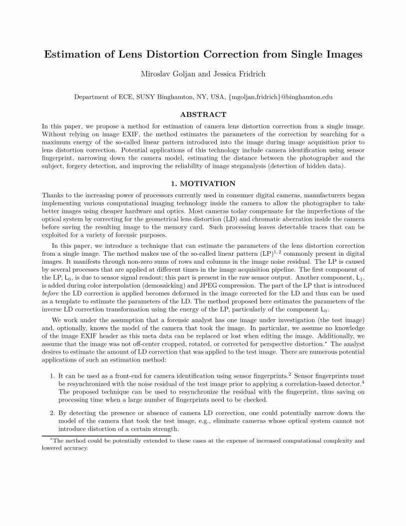
Figure 1 shows an example of L after scaling its elements to the range [0, 255] to obtain a grayscale image. Notethat the linear pattern of L is again the same set {c, r}, L(L) = L(X), which justifies why we do not alwaysdifferentiate between the two forms, L and L, when speaking about the same linear pattern in this paper.

‡The method would still work if the image was resized and / or centrally cropped.§Although not introduced in this paper, the proposed method can be applied to individual color channels to make it

work when the camera corrects for chromatic aberration.

Figure 1. Left: Close up of a linear pattern L obtained from one test image from Nikon S9100. Right: Padded borderarea (gray) appears after the barrel distortion. The LP is computed only from the inner rectangle.

The energy of the linear pattern L = {c, r} is defined as the sum of squares of L2 norms of c and r:

E(L) = ‖c‖2+ ‖r‖2

=

n∑

j=1

c2j +

m∑

i=1

r2i . (5)

3.2 Parameters estimation as an optimization problem

Typically, cameras correct for barrel distortion at the wide-angle end of the zoom (short focal length). The cameraapplies the inverse of the barrel transform – the pin-cushion transform. In order to undo this correction, we haveto apply the original barrel distortion or, more precisely, the inverse transform to the pin-cushion correction.Notice that the image dimensions and shape change as the content may shrink or expand during the transform(see Figure 1 right). This affects the computed LP and its energy (5) because the mean values calculated fromthe columns and rows of W get smaller with increasing barrel distortion when padding to the original dimensionswith zeros. Working with all valid samples (the white area in Figure 1 right), on the other hand, creates problemsdue to the large fluctuations of mean values of short columns and rows, which often leads to false peaks in the LPenergy. In order to avoid these unwanted border effects, we restrict all LP computations to the largest rectangleof dimensions m′ × n′ inscribed into the transformed image (Figure 1 right). The parameters a = (a2, a4) of theLD correction transform Ta (2) are estimated by applying an inverse mapping, T −1

a, to W and searching for the

maximum of the energy of its linear pattern (5) as a function of a.

The inverse LD correction transform, T −1a

, was implemented in the following manner. The value of pixelx at distance r from the image center is calculated by interpolating four pixels in the image with the nearestinteger coordinates of pixel x′ at distance r′ given by Eq. (2) and in the same direction from the center. Bilinearinterpolation method was chosen for its speed as it is utilized repeatedly during the search. To avoid transformingthe image a number of times and recalculating its noise residual, the inverse transforms T −1

awere applied directly

to the noise residual W.

It is worth pointing out that the main driving parameter is a2. The parameter a4 is responsible for “finetuning” the transform and starts playing its role for pixels farther away from the image center, typically morethan 1/4 of the image diagonal. This allows for a two-stage search – first running a grid search for a2, whichis followed by a two-parameter search to determine both a2 and a4. A suitable optimization method for thisproblem is the Nelder-Mead method14 because it is robust to noise in our objective function (see Figure 2).

During the first stage, we can either fix the value of a4 or adopt some functional dependence of a4 on a2

in order to have a single-parameter search. (See Section 3.3 for more details.) When the distortion is small,a2 ≈ 0, the LP energy L(T −1

a(W)) mostly depends on L1. Hence, we cannot reliably estimate a2 when it is

small, which is why we restrict the search interval to a2 ∈ [amin, amax], amin > 0. In the first stage, we fit asecond-degree polynomial to E(L(T −1

(a2,0)(W))) as a function of a2 and compute the difference 4E(a2) between

the LP energy and the polynomial fit. Then, we locate the maximum of this difference, say, found at a(1)2 (see

0 0.05 0.1 0.15 0.2 0.25 0.3 0.35−0.1

0

0.1

2

2.5

3

3.5

a4

a2

E

0 0.05 0.1 0.15 0.2 0.25 0.3 0.35−0.1

0

0.1

2

2.5

3

3.5

4

4.5

5

5.5

a4

a2

E

Nikon S9100 Canon PS SX 40HSFigure 2. Linear pattern energy vs. radial transform parameters for two cameras.

an example in Figure 4). After obtaining the rough estimate a(1)2 , we use it for a three-point initialization of

the Nelder-Mead optimization by setting a(1) = (x, x2), a

(2) = (x, −x2), and a(3) = (0.8x, 0), where x = a

(1)2 .

During the optimization, both parameters (a2, a4) are determined by the maximum of the objective function:

f(a2, a4) = E(

L(

T −1(a2,a4)(W)

)). (6)

The reason for subtracting the second-order polynomial fit is the following. The objective function (6) as afunction of a2 (under a4 = 0) is non-monotone and non-linear. Our goal is to find its local peak correspondingto the true LD correction parameters even if this peak does not attain the global maximum value of f . Fittinghigher-order polynomials would lead to over fitting.

Due to the noise in the objective function, the above estimation procedure always finds some maximum, whichwill occur at a2 6= 0, even when no LD correction was applied. Thus, the estimation needs to be augmented witha routine that would decide when the distortion correction has not occurred, i.e., when a = 0. To this end, weevaluate the so-called “significance of the peak” at a = (a2, a4). First, the objective function (6) is evaluated atfour colinear points in the neighborhood of a: (a2i, a4i), a2i = a2 + 0.01i, a4i = a4

a2i

a2

, i = −2, −1, 1, 2. After

including the fifth point (a2i, a4i) = (a2, a4), i = 0, where the objective function (6) was already evaluated, asecond-degree polynomial A ‖a‖ 2 +B ‖a‖+C is fit to these five points using the least square method (Figure 3).The peak significance s is defined as s = −A. The peak is called “significant” if s > t , 180(α + 1/α)2,where α = m/n is the image aspect ratio. The form of this threshold is dictated by the expected energy of aresidual that does not contain any LP. Modeling such a residual as a zero-mean matrix whose elements are i.i.d.realizations of a random variable with finite variance σ2, the expected value of its LP energy is (α + 1/α)σ2

(Appendix 6), which only depends on the image aspect ratio but not the image dimensions. The value of themultiplicative threshold was chosen by analyzing 555 images from three camera models to obtain the rate of≈ 3% of not correctly recognizing the case when no LD correction was applied.

This way, peaks that are not significant are deemed as random fluctuations rather than due to the presenceof a LP, and our routine decides that no LD correction was applied, a = 0.

3.3 List of improvements

The proposed parameter estimation method solely relies on the strength of the linear pattern, which is a veryweak signal. In the process, the LP is transformed twice, once with Ta and once with T −1

a. In practice, these

two mapping are only approximately inverse to each other even when a = a because each transform has to applysome kind of interpolation when evaluating the pixel values on the regular lattice. Inverting this interpolation is

0 0.05 0.1 0.15 0.2 0.25 0.3−0.1

−0.05

0

0.05

0.1

a2

a4

(a2, a4)

Peak sampling direction

Grid search

0 0.05 0.1 0.15 0.2 0.25 0.31

1.5

2

2.5

3

||a||

E

A(||a||)2 + B(||a||) +C

(a) (b)Figure 3. Sampled points (a2i, a4i), i = 0, . . . , 4 (a), the peak significance is defined as s = −A (b). See text for moredetails.

0 0.05 0.1 0.15 0.2 0.25 0.3 0.350

0.5

1

1.5

2

2.5

3

3.5

4

a2

E Polymomial fit

First stage maximumFinal optimum foundby Nelder−Mead method

a2(1)

Figure 4. Example of the grid search in the first stage and the optimal (peak) value from the second stage for a test imagefrom Canon PS SX 40HS taken at focal length = 5.649 mm, a2 = 0.130, a4 = −0.0145.

not perfect either because the interpolation method (its kernel) is not publicized by camera manufacturers andmay vary across camera models. The image content is another factor that influences the results of the proposedmethod.

To alleviate the above issues, we investigated several potential improvements, which we divide into subsectionsbased on their effectiveness.

3.3.1 Realized improvements

In this subsection we expose the details of the method implementation as it was used to carry our experimentsin Section 4.

First of all, the image noise residual W as well as its every transformed form T −1a

(W) is normalized to a unitsample variance before the LP energy is computed. This step makes the optimized objective function “betterbehaved.”

In order to avoid the strong influence of the component L1, which was introduced after the LD correction, onthe measured LP energy, we subtract it before applying the inverse transform, and we measure only the residualenergy of L0. A drawback of this approach is that we cannot completely separate L1 from L0. Subtracting theLP from W not only eliminates L1 but also suppresses L0 in the central part in the image, where the distortion

is the smallest. If no LD correction is applied, both components of the LP are subtracted fully, which meansthat a small LD correction is harder to estimate than a large one.

A partial remedy to this problem is a variation of this approach. Instead of subtracting the entire LP,W = W − L(W), we really wish to subtract only a certain “scaled amount” of L(W) to obtain a residual whoseLP energy would correspond to an undistorted residual with no LP. The expected LP energy of a random matrixwhose elements are i.i.d. realizations of a random variable with variance σ2 is (α + 1/α)σ2, where α = m/n isthe aspect ratio of W (Appendix 6). Estimating σ2 as the sample variance of W, it is shown in Appendix thatby transforming W in the following manner:

W = [wi,j ]m,n

i,j=1 , wi,j = wi,j − cj − ri + cj

1

‖c‖

√nσ2

m+ ri

1

‖r‖

√mσ2

n, (7)

we give the resulting residual W the required energy (α + 1/α)σ2. In (7), cj , ri are as defined by (4). Theadvantage of this transform of W manifests itself primarily when the test image has not been corrected for LD asin this case near a2 = 0 the energy E (L(W)) exhibits a false peak, E(L(W)) = 0, while E(L(W)) = (α+1/α)σ2.

In order to reduce the possibility of missing the peak in the LP energy, we implemented the following measure.The first search over a2 is run twice: for a4 = a2

2 and a4 = −a22. This dependence a4(a2) was chosen empirically

from experiments based on the observed relationship between both parameters. The optimal value of a4 mostlyhappens to lie between these two values, still including the possible (and likely) case when a4 = 0. Thus, we

obtain two intermediate estimates, from which we choose the one having the larger 4E and denote it as a(2)2 .

This estimate replaces a(1)2 , while the choice of the initial points for the Nelder-Mead optimization remains as

described in Section 3.2.

3.3.2 Possible improvements

Here, we list a few ideas that did not consistently improve our test results but may be worth investigating.

1. Replacing E(L) (5) with E4(L) defined as follows. Start with breaking down the noise residual W =[wi,j ]m,n

i,j=1 into four sub-matrices corresponding to four pixel types determined by the Bayer Color Filter Array

(CFA),6 normalizing them to a unit sample variance, and evaluating the total energy as the sum of energies ofall four sub-matrices. The total energy derived from W (assuming n, m even) is

E4(L) =

4∑

k=1

E (L(Wk/σk)) , (8)

W1 = [wi,j ], i = 1, 3, ..., m − 1; j = 1, 3, ..., n − 1,

W2 = [wi,j ], i = 2, 4, ..., m; j = 1, 3, ..., n − 1,

W3 = [wi,j ], i = 1, 3, ..., m − 1; j = 2, 4, ..., n,

W4 = [wi,j ], i = 2, 4, ..., m; j = 2, 4, ..., n,

whereσ2

k = V ar(Wk), k = 1, . . . , 4, (9)

are the sample variances computed from all elements of the matrices Wk. The normalization by the standarddeviation equalizes the contribution of each pixel type to the total energy E.

2. Normalizing E (5) by 1n′+m′

, where n′ and m′ are the dimensions of the largest rectangle inscribed

into T −1a

(W). This would make sense as E may be intuitively expected to decrease with decreasing n′ and m′.However this is not generally true and it may depend on the properties of the interpolation method. We observedthat E was not decreasing when T −1

a(W) was evaluated using bi-linear interpolation.

3. It remains unclear whether a more advanced interpolation may bring any improvement unless it perfectlyinverts the original interpolation applied in the camera. However, camera manufactures do not reveal this levelof detail about their in-camera processing. Moreover, perfect inversion will never be possible as some informationwill always be lost due to additional in-camera image processing, which includes the JPEG compression.

0 0.05 0.1 0.15 0.2 0.25 0.3 0.353

3.5

4

4.5

5

5.5

6

6.5

7

7.5

8

a2

E

0 0.05 0.1 0.15 0.2 0.25 0.3 0.351

1.5

2

2.5

3

3.5

4

4.5

5

a2

log 10

(PC

E)

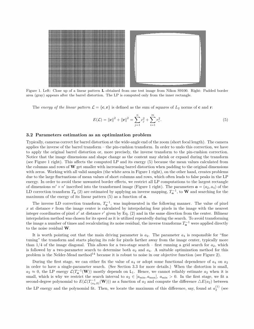
Maximizing LP energy Maximizing PCEFigure 5. Example of an independent verification of the estimated parameter a2 for an image from Canon PS SX 230HSwhen maximizing the LP energy and the PCE.

We note that we considered skipping the first-stage grid search, which would significantly improve computa-tion time. However, in this case, we were not able to initialize the Nelder-Mead optimization to consistently findthe desired maximum and avoid being trapped in an incorrect local maximum.

3.4 Ground truth

In order to evaluate the accuracy of the proposed estimation procedure, we need to know the ground truth. Tothis end, we employed an independent method of LD estimation based on camera fingerprints matching.4 First,we estimate the camera fingerprint F from images that did not undergo LD, e.g., images with focal length at 20mm or larger for our tested cameras. The PCE (1) between F and T −1

a(W), PCE

(F, T −1

a(W)

), is maximized

at the true value of a.

For the three cameras that we had access to, i.e., Canon PS SX 230HS, Nikon S9100, and Panasonic DMC ZS7,we estimated the camera fingerprint from ten flat field images at focal length near 20 mm using the maximumlikelihood estimator.2 The PCE (1) was collected along with the LP energy during each search for the parametera. We observed that the points in the parameter space that maximized the LP energy and the PCE were alwaysvery close to each other.

To provide an additional insight and evidence, we executed the search algorithm as described in Sections 3.2–3.3.1 with the objective function (the LP energy) replaced with log10(PCE(F, T −1

a(W))). Figure 5 shows an

example of the PCE on the log scale evaluated at different values of a during the search. The output of thisalgorithm is an alternative estimate of a, which we expect to be of higher precision thanks to the side informationin the form of the camera fingerprint. This is confirmed by contrasting the statistical spread of the estimatesobtained using PCE as the objective function in Figure 6 with Figure 7 showing the results for the proposedmethod.

The problem with uncertain ground truth can be eliminated altogether if our goal is estimating the focallength instead of the parameters of the LD correction. This is possible if the relationship between the focallength and the parameter a2 is known. Estimating focal length will have one obvious limitation – one will notbe able to obtain the focal length estimate when no LD correction is applied (typically when the focal length isabove 9–11 mm).

4. EXPERIMENTS

To test the proposed estimation procedure, we prepared a database of images from three cameras made byCanon, Nikon, and Panasonic, as well as images from three other Canon and Nikon models downloaded fromthe Flickr image sharing portal (see Table 1). For the first three cameras, we also prepared their fingerprints ofcomparable quality obtained from ten flat field exposures to independently verify the results. All test images

4 5 6 7 8 9 10 110

0.05

0.1

0.15

0.2

0.25

Focal length (mm)

a2

4 5 6 7 8 9 10 110

0.05

0.1

0.15

0.2

0.25

Focal length (mm)

a2

Canon SX230 HS Nikon S9100Figure 6. Parameter a2 as a function of focal length estimated by maximizing PCE(F, T −1

a(W)) for two cameras. The

crosses correspond to individual images.

Camera Model Zoom (mm) Sensor Test Images (#) fc Image Dimension

Canon PS SX 230HS 5.0 – 70 12.1 Mp CMOS 100 + 89 11.2 3000 × 4000Nikon S9100 4.5 – 81 12.1 Mp CMOS 150 + 39 11.2 3000 × 4000Panasonic DMC ZS7 4.1 – 49.2 12.1 Mp CCD 91 + 86 8.0 3000 × 4000Canon PS SX 210IS 5.0 – 70 14.1 Mp CCD 80 + 44 (F) 11.2 3240 × 4320Canon PS SX 40HS 4.3 – 150.5 12.1 Mp BSI-CMOS 62 + 96 (F) 9.0 3000 × 4000Nikon P510 4.3 – 180 16.1 Mp CMOS 82 + 18 (F) 9.0 3456 × 4608

Table 1. Camera models and test images. Images downloaded from Flickr are marked by (F).

were acquired at the full resolution as indicated in Table 1, at varying focal lengths, and were chosen randomlyfrom a larger number of images available. The number of test images indicated in this table is split to imageswith focal length that is below/above a cut-off focal length fc. The cut-off is an approximate value above whichthe LD correction is not present.¶

The grid search for parameter a2 was run for 60 equidistant samples on the interval [0.0.3]. We set amin = 0.01and amax = 0.30. Figure 7 shows the estimated leading parameter a2 vs. the image focal length retrieved fromthe image EXIF header. The plotted data points are only those obtained from significant peaks. The focal lengthinformation helps us determine the ground truth needed for evaluating the results. Although we do not knowthe exact relationship between a2 and the focal length, we can assume that this relationship does not includeany other hidden parameters. Therefore, the parameter a2 should fall on one curve when estimated from imagescoming from the same camera (or more cameras of the same model). For illustration, the dependence of a2 onthe focal length is rendered by a dotted line connecting the median estimate values for each focal length. Thesefigures only include images with focal length below fc where the LD correction was apparently detected.

The results from images with focal length above fc are not shown because most of these images were correctlyrecognized as having an undistorted LP, i.e., a2 = 0 (and by default a4 = 0). A small number of incorrectlyestimated parameters were encountered for images that were corrected for LD. These errors can be seen asoutliers in Figure 7 and their numbers are shown in the rightmost column of Table 2.

¶The knowledge of the cut-off focal length is not used in the process of parameters estimation.

4 5 6 7 8 9 10 110

0.05

0.1

0.15

0.2

0.25

Focal length (mm)

a2

4 5 6 7 8 9 10 110

0.05

0.1

0.15

0.2

0.25

Focal length (mm)

a2

Canon SX230 HS Nikon S9100

4 5 6 7 8 9 10 110

0.05

0.1

0.15

0.2

0.25

Focal length (mm)

a2

4 5 6 7 8 9 10 110

0.05

0.1

0.15

0.2

0.25

Focal length (mm)

a2

Panasonic DMC ZS7 Canon PS SX 210IS

4 5 6 7 8 9 10 110

0.05

0.1

0.15

0.2

0.25

Focal length (mm)

a2

4 5 6 7 8 9 10 110

0.05

0.1

0.15

0.2

0.25

Focal length (mm)

a2

Canon PS SX 40HS Nikon P510Figure 7. Estimated parameter a2 as a function of the focal length for six cameras.

Experiments revealed that the performance of the presented method varies significantly across camera makesand models. This is captured with the “correct estimation” rates in Table 2. This rate was between 60–80% for

Camera Model Correct Estimation Incorrect Estimation Missed No-LD

Canon PS SX 230HS 62/100 2/100 2/89Nikon S9100 102/150 1/150 7/39

Panasonic DMC ZS7 30/91 4/91 6/86Canon PS SX 210IS 56/80 0/80 0/44Canon PS SX 40HS 50/62 0/62 7/96

Nikon P510 11/82 1/82 0/18

Table 2. The number of correctly / incorrectly estimated a2 for images in the LD correction range and missed cases of noLD correction.

images from four out of six camera models, while the LD correction in images from Nikon P510 and PanasonicDMC ZS7 was the hardest to detect and estimate.

This method may not be universally applicable. We ran tests for images downloaded from Flickr thatoriginated from Sony DSC-H70, a camera equipped with a 16.1 Mp Super HAD CCD imaging sensor. The testresults were mostly failures for this camera. We hypothesize that this might have been caused by a different lensdistortion model used by the manufacturer.

The experiments point out an advantage of the two-parameter model over the one-parameter model (a2 only)in its ability to output the parameter a2 with a smaller error (not shown in this work), rather than in its abilityto estimate a4. The two-parameter model may produce less accurate results when the camera on-board softwareuses a one-parameter radial transform (a4 = 0).

5. CONCLUSION

Digital images are increasingly often used as inputs for forensic analysis, data mining, and intelligence gathering.Digitally represented data can be, however, subjected to a variety of processing that might affect its semanticmeaning and value, which may in turn negatively impact its interpretation and lead to erroneous decisions.Techniques that can reveal the processing history of digital media are thus of crucial importance. In this paper,we describe another tool for the forensic expert toolbox – one that can blindly estimate from a single imagethe parameters of a lens-distortion correction applied to it. Since the vast majority of today’s compact digitalcameras employ the lens distortion correction as part of their in-camera (or off-line) processing, the proposedmethod can help investigators narrow down the camera that took a given image, reveal portions of the imagethat have been replaced or maliciously modified, estimate the focal length at which the image was taken andthus establish the distance between the scene and the photographer. Knowing that an image was corrected forlens distortion may also be useful when analyzing it for presence of steganographically embedded data.

The proposed method uses the so-called linear pattern inserted into the image during the acquisition. Thispattern, which is originally a set of orthogonal lines, gets distorted when a lens distortion correction is applied. Weuse it as a template to estimate the lens distortion correction parameters. In particular, when the (approximately)same inverse distortion is applied, the pattern again becomes rectilinear, which manifests itself in the increasedenergy of pixels’ row and column means. Maximizing this energy w.r.t. parameters of the lens distortion enablesus to estimate the distortion correction without the need for any other auxiliary information. The proposedmethod works from a single image. Tests on images coming from six cameras showed that this method canreasonably accurately estimate the applied lens distortion correction.

The method as proposed only works under some simplifying assumptions, namely that no other geometricaltransformation, besides scaling or centralized cropping, was applied to the image. In principle, at the expenseof computational complexity and somewhat less accurate performance, the approach could be extended to im-ages that were additionally off-center cropped, rotated, or corrected for perspective distortion. The proposedmethod may not work reliably for heavily processed images, such as aggressive denoising or low-quality JPEGcompression, because the template signal, the linear pattern, is relatively weak.

6. ACKNOWLEDGMENTS

The work on this paper was supported by Air Force Office of Scientific Research under the research grant numberFA9950-12-1-0124. The U.S. Government is authorized to reproduce and distribute reprints for Governmentalpurposes notwithstanding any copyright notation there on. The views and conclusions contained herein are thoseof the authors and should not be interpreted as necessarily representing the official policies, either expressed orimplied, of AFOSR or the U.S. Government.

Appendix A

If X is a random matrix with elements i.i.d. realizations of a zero-mean random variable with variance σ2, theexpected value of its LP energy E (L(X)) is (α + 1/α)σ2, where α = m/n is the aspect ratio of X. This followsimmediately from the fact that cj ∼ N(0, σ2/m) for all j = 1, . . . , n and ri ∼ N(0, σ2/n) for all i = 1, . . . , m:

E

n∑

j=1

c2j +

m∑

i=1

r2j

=

n∑

j=1

E{c2j} +

m∑

i=1

E{r2j } = n × σ2

m+ m × σ2

n. (10)

Let [zi,j ]m,ni,j=1 be an arbitrary zero-mean matrix with linear pattern L(Z) = {r, c}. Let G = [gi,j ]m,n

i,j=1,

gi,j =cj

‖c‖

√nσ2

m+ ri

‖r‖

√mσ2

n. Then, the energy of the linear pattern of Y = [yi,j ], yi,j = zi,j − cj − ri + gi,j , is

E(L(Y)) =

n∑

j=1

(1

m

m∑

i=1

yi,j

)2

+

m∑

i=1

1

n

n∑

j=1

yi,j

2

(11)

=

n∑

j=1

(1

m

m∑

i=1

(zi,j − cj − ri) +1

m

m∑

i=1

gi,j

)2

+

m∑

i=1

1

n

n∑

j=1

(zi,j − cj − ri) +1

n

n∑

j=1

gi,j

2

(12)

=

n∑

j=1

(1

m

m∑

i=1

gi,j

)2

+

m∑

i=1

1

n

n∑

j=1

gi,j

2

=( n

m+

m

n

)σ2, (13)

because

m∑

i=1

(zi,j − cj − ri) =m∑

i=1

(zi,j − 1

m

m∑

i=1

zi,j

)− 1

n

m,n∑

i,j=1

zi,j = 0 ∀j = 1, . . . , n, (14)

and, similarly,∑n

j=1(zi,j − cj − ri) = 0 for all i = 1, . . . , m. Moreover,

n∑

j=1

(1

m

m∑

i=1

gi,j

)2

=

n∑

j=1

(1

m

m∑

i=1

cj

‖c‖

√nσ2

m+

ri

‖r‖

√mσ2

n

)2

=

n∑

j=1

nσ2

m

c2j

‖c‖2 = nσ2

m, (15)

and similarly∑m

i=1

(1n

∑n

j=1 gi,j

)2

= mσ2/n.

REFERENCES

1. M. Chen, J. Fridrich, and M. Goljan. Digital imaging sensor identification (further study). In E.J. Delpand P.W. Wong, editors, Proc. SPIE, Electronic Imaging, Security, Steganography, and Watermarking of

Multimedia Contents IX, volume 6505, pages 0P–0Q, San Jose, California, January 28–February 1, 2007.

2. J. Fridrich. Digital image forensic using sensor noise. IEEE Signal Processing Magazine, 26(2):26–37, 2009.

3. J. Fridrich, J. Kodovský, M. Goljan, and V. Holub. Breaking HUGO – the process discovery. In T. Filler,T. Pevný, A. Ker, and S. Craver, editors, Information Hiding, 13th International Conference, volume 6958of Lecture Notes in Computer Science, pages 85–101, Prague, Czech Republic, May 18–20, 2011.

4. M. Goljan and J. Fridrich. Sensor-fingerprint based identification of images corrected for lens distortion.In N. Memon, A. Alattar, and E. Delp III, editors, Proceeedings of SPIE, Electronic Imaging, Media Wa-

termarking, Security, and Forensics 2012, volume 8303, pages 0H 1–13, San Francisco, CA, January 23–25,2012.

5. G. Gül and F. Kurugollu. A new methodology in steganalysis : Breaking highly undetactable steganograpy(HUGO). In T. Filler, T. Pevný, A. Ker, and S. Craver, editors, Information Hiding, 13th International

Conference, volume 6958 of Lecture Notes in Computer Science, pages 71–84, Prague, Czech Republic, May18–20, 2011.

6. J. R. Janesick. Scientific Charge-Coupled Devices, volume Monograph PM83. Washington, DC: SPIE Press,The International Society for Optical Engineering, January 2001.

7. M.K. Johnson and H. Farid. Exposing digital forgeries through chromatic aberration. In J. Fridrich andJ. Dittmann, editors, Proceedings of the 8th ACM Multimedia & Security Workshop, pages 48–55. ACMPress, New York, September 26–27, 2006.

8. J. Kodovský and J. Fridrich. Steganalysis in resized images. In Proc. of IEEE ICASSP, pages 2857–2861,Vancouver, Canada, May 26–31, 2013.

9. J. Kodovský, V. Sedighi, and J. Fridrich. Study of cover source mismatch in steganalysis and ways to mitigateits impact. In A. Alattar, N. D. Memon, and C. Heitzenrater, editors, Proceedings SPIE, Electronic Imaging,

Media Watermarking, Security, and Forensics 2014, volume 9028, San Francisco, CA, February 3–5, 2014.

10. I. Lubenko and A. D. Ker. Steganalysis with mismatched covers: Do simple classifiers help? In J. Dittmann,S. Katzenbeisser, and S. Craver, editors, Proceedings of the 14th ACM Multimedia & Security Workshop,pages 11–18, Coventry, UK, September 6–7, 2012. ACM Press, New York.

11. J. Lukáš, J. Fridrich, and M. Goljan. Digital camera identification from sensor pattern noise. IEEE

Transactions on Information Forensics and Security, 1(2):205–214, June 2006.

12. M.K. Mihcak, I. Kozintsev, K. Ramchandran, and P. Moulin. Low-complexity image denoising based onstatistical modeling of wavelet coefficients. IEEE Signal Processing Letters, 6(12):300–303, December 1999.

13. A.C. Popescu and H. Farid. Exposing digital forgeries by detecting traces of resampling. IEEE Transactions

on Signal Processing, 53(2):758–767, February 2005.

14. W. H. Press, S. A. Teukolsky, W. T. Vetterling, and B. P. Flannery. Numerical Recipes 3rd Edition: The

Art of Scientific Computing. Cambridge University Press, New York, NY, USA, 3 edition, 2007.

15. H. Wolfgang. Correcting lens distortions in digital photographs. 2010.http://www.imagemagick.org/Usage/lens/correcting_lens_distortions.pdf.