Estimation of Underwater Noise - a simplified...

Estimation of Underwater Noise -a simplified method

- theory derived to support practical work on Environmental Impact Assessments in collaboration with Metoc plc.To be published in Underwater Technology 26/3 (2005)

Dr Dick Hazelwood M.I.O.A.R & V Hazelwood Associates LLP

Guildford U.K.

Underwater Noise Measurement SeminarNPL 13th Oct 2005

R & V Hazelwood Associates, Guildford U.K.

The complexities of EIAs

There are many difficulties encountered in making an Environmental Impact Assessment which is to include underwater noise. In this work, simpler solutions have been sought to the following aspects -Assess the power of the noise sources. This topic was the subject of an article in the Institute of Acoustics Bulletin 2005 and earlier presentations such as MMF #34.Estimate how the noise is propagated. This topic alone has had many years of worldwide research, so very complex.Estimate the likely background noise pressure levelsRelate these findings to the sensitivity of the receptors.


The need for simplifications in EIAs

After the 2003 Marine Measurement Forum, I was involved in consultative work for Metoc plc , for a cable laying project between the UK and the Netherlands.Metoc had found it impossible to get appropriate data on the likely noise sources, especially those of the underwater equipment such as trenching tools. Despite many discussions, we still need better ways for such data to be disseminated in a practically useful way. Data from commercial surveys tends to be confidential, as does much military work. Much of the confidential detail is not required for preliminary “coarse” assessments, but agreed simplifications would be required.


The balance between simplicity and accuracy.

Prediction of noise pressure levels to be generated by future operations is necessarily very approximate. Any relatively simple survey must be viewed as preliminary, unless it can show that risks are minimal.

However, the current complexity does not help in general understanding, generating unnecessary concerns. Facilitating a “rough cut” or “ball park” analysis should allow attention to be concentrated on the serious issues, and minimise unnecessary restrictions on much needed projects.

.


Simple source characterisation - the linkage to acoustic wattage

Urick’s “Principles of Underwater Sound” includes many valuable simplifications which can usefully be revisited.

For ship noise he shows how it is possible to quote the total acoustic wattage emitted into the sea. To be able to do this involves several assumptions - the directivity and frequency distribution of the noise in particular.Since the orientation of a ship in future operations is unknown, the average emission over all directions is used.The high frequency “roll-off” is taken as “red” noise (or “1/f²” noise). This is known to be a good approximation.The low frequency noise is assumed to be “white”, an average of an ensemble of ships, smoothing tonal noise.


A noise criterion for fish survey ships - ICES report #209 ,1995

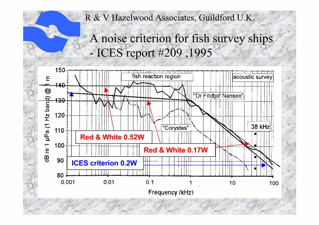
Red & White 0.52W

ICES criterion 0.2W

Red & White 0.17W


The ICES model and its relation to “red & white” noise

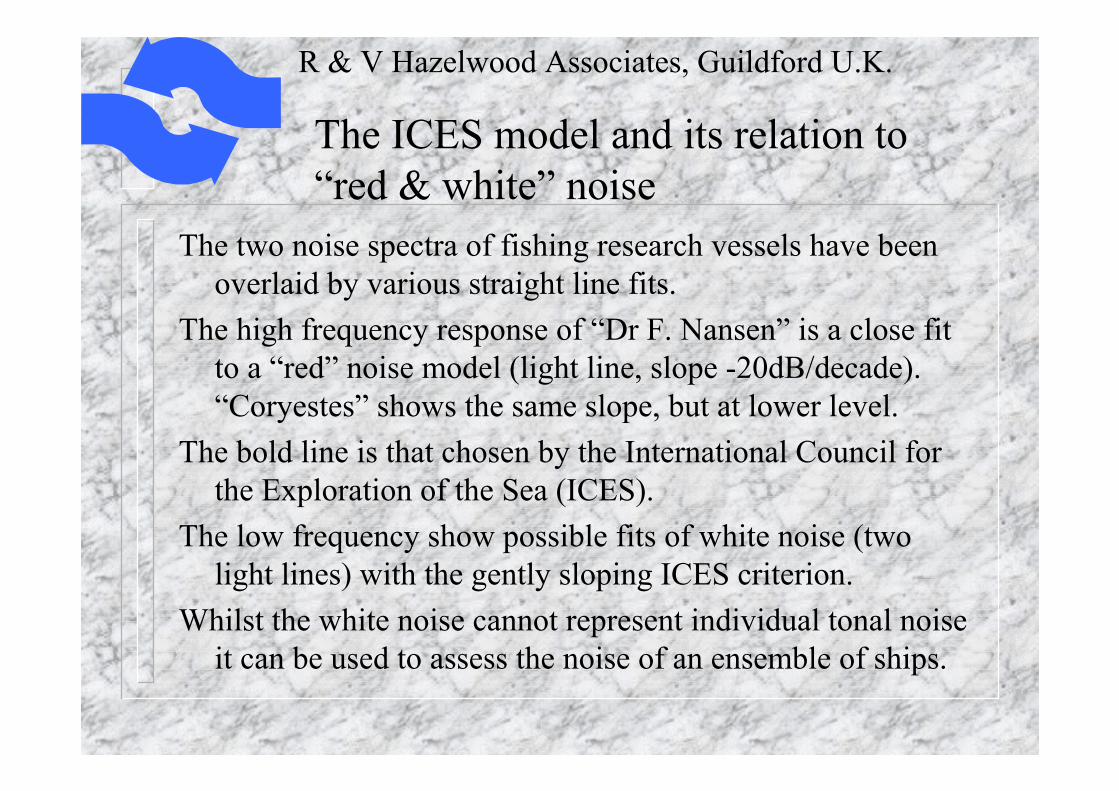
The two noise spectra of fishing research vessels have been overlaid by various straight line fits.

The high frequency response of “Dr F. Nansen” is a close fit to a “red” noise model (light line, slope -20dB/decade). “Coryestes” shows the same slope, but at lower level.

The bold line is that chosen by the International Council for the Exploration of the Sea (ICES).

The low frequency show possible fits of white noise (two light lines) with the gently sloping ICES criterion.

Whilst the white noise cannot represent individual tonal noise it can be used to assess the noise of an ensemble of ships.


The calculation of total noise power

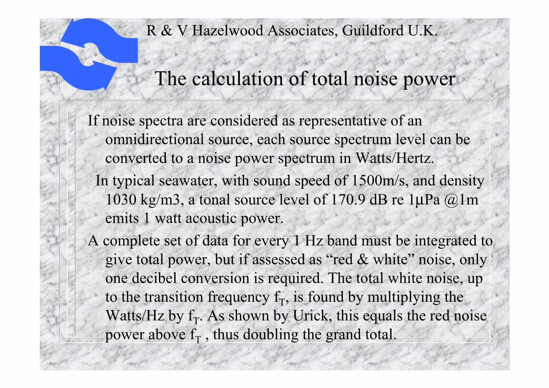
If noise spectra are considered as representative of an omnidirectional source, each source spectrum level can be converted to a noise power spectrum in Watts/Hertz.

In typical seawater, with sound speed of 1500m/s, and density 1030 kg/m3, a tonal source level of 170.9 dB re 1µPa @1m emits 1 watt acoustic power.

A complete set of data for every 1 Hz band must be integrated togive total power, but if assessed as “red & white” noise, only one decibel conversion is required. The total white noise, up to the transition frequency fT, is found by multiplying the Watts/Hz by fT. As shown by Urick, this equals the red noise power above fT , thus doubling the grand total.


An alternative graphical presentation

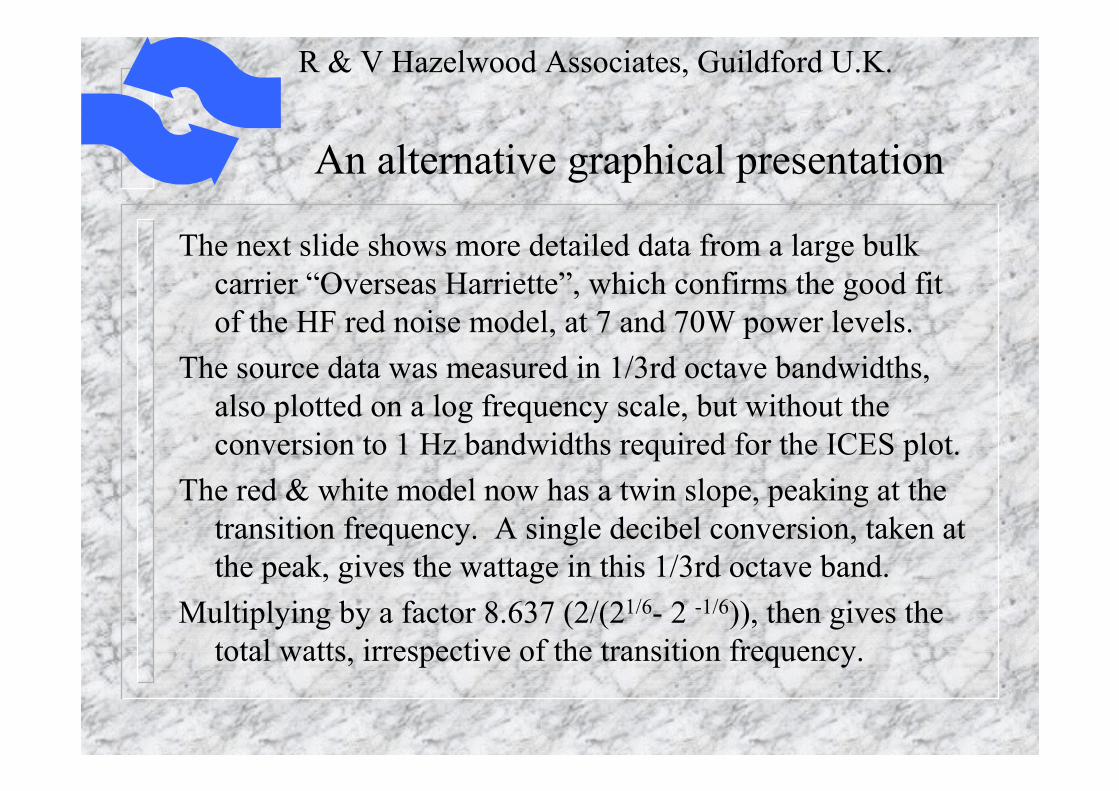
The next slide shows more detailed data from a large bulk carrier “Overseas Harriette”, which confirms the good fit of the HF red noise model, at 7 and 70W power levels.

The source data was measured in 1/3rd octave bandwidths, also plotted on a log frequency scale, but without the conversion to 1 Hz bandwidths required for the ICES plot.

The red & white model now has a twin slope, peaking at the transition frequency. A single decibel conversion, taken at the peak, gives the wattage in this 1/3rd octave band.

Multiplying by a factor 8.637 (2/(21/6- 2 -1/6)), then gives the total watts, irrespective of the transition frequency.


Bulk carrier noise (publ J.A.S.A. 2000)

Red & White 70W

Red & White 7W


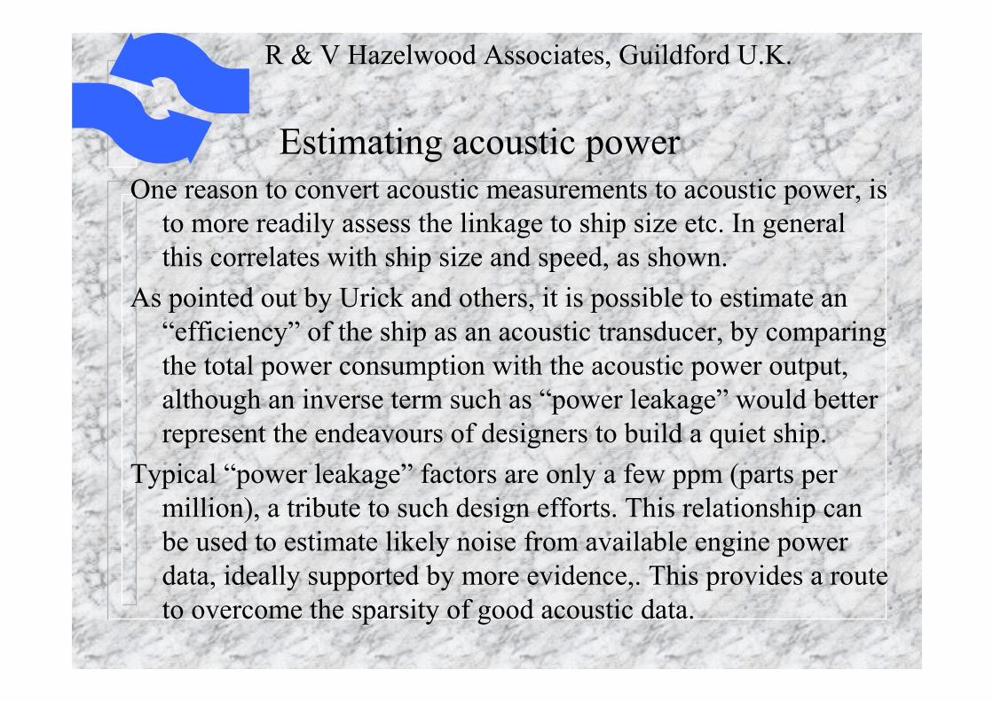
Estimating acoustic powerOne reason to convert acoustic measurements to acoustic power, is

to more readily assess the linkage to ship size etc. In general this correlates with ship size and speed, as shown.

As pointed out by Urick and others, it is possible to estimate an “efficiency” of the ship as an acoustic transducer, by comparingthe total power consumption with the acoustic power output, although an inverse term such as “power leakage” would better represent the endeavours of designers to build a quiet ship.

Typical “power leakage” factors are only a few ppm (parts per million), a tribute to such design efforts. This relationship can be used to estimate likely noise from available engine power data, ideally supported by more evidence,. This provides a routeto overcome the sparsity of good acoustic data.


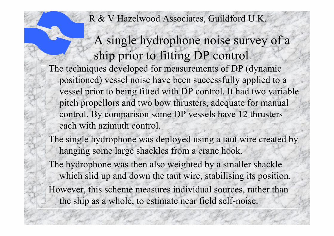
A single hydrophone noise survey of a ship prior to fitting DP control

The techniques developed for measurements of DP (dynamic positioned) vessel noise have been successfully applied to a vessel prior to being fitted with DP control. It had two variable pitch propellors and two bow thrusters, adequate for manual control. By comparison some DP vessels have 12 thrusters each with azimuth control.

The single hydrophone was deployed using a taut wire created by hanging some large shackles from a crane hook.

The hydrophone was then also weighted by a smaller shackle which slid up and down the taut wire, stabilising its position.

However, this scheme measures individual sources, rather than the ship as a whole, to estimate near field self-noise.


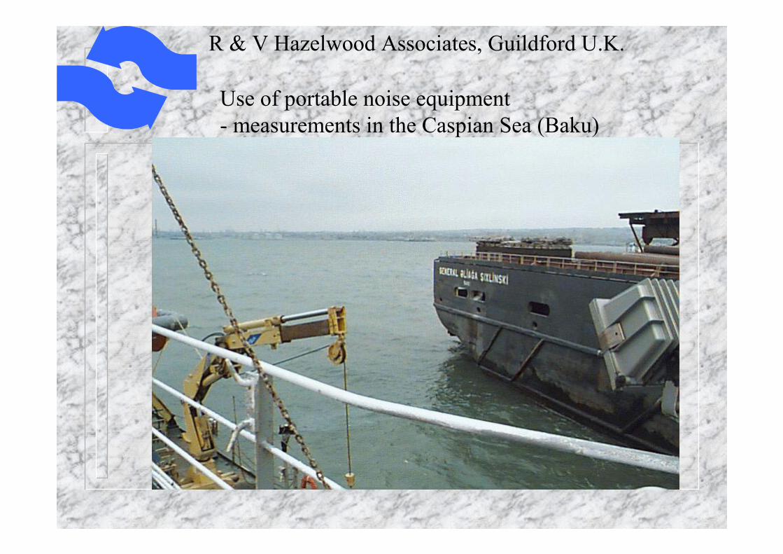
Use of portable noise equipment - measurements in the Caspian Sea (Baku)


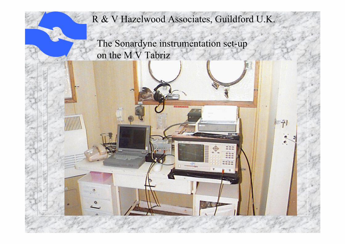
The Sonardyne instrumentation set-upon the M V Tabriz


Noise from underwater machinery

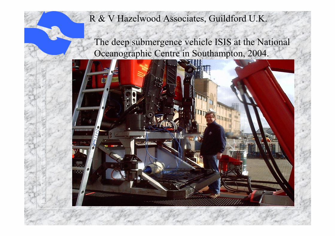
Whilst data from subsea machinery may be confidential, some results are given here from a recent noise measurement made on the deep ocean ROV “ISIS”, by permission of NOC.

Unlike many other work class ROVs, this has electric motor propulsion, although still retaining hydraulic tooling.

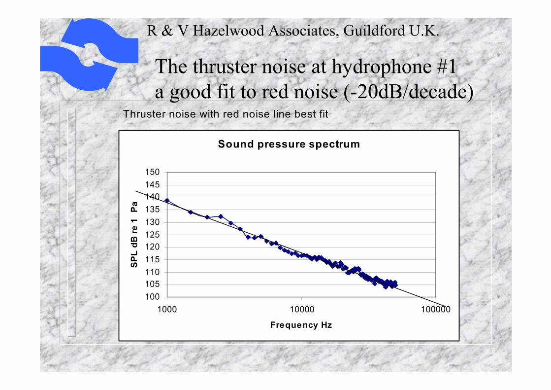
The propulsion noise is seen to closely fit a red noise model, at the frequencies measured.

In contrast, the noise from the hydraulic pump was more nearly white to frequencies above 50kHz .

Whilst red & white models may be applicable to both sources, the data is inadequate to determine transition frequencies.


The deep submergence vehicle ISIS at the National Oceanographic Centre in Southampton, 2004.


The thruster noise at hydrophone #1a good fit to red noise (-20dB/decade)

Thruster noise with red noise line best fit

Sound pressure spectrum

100105110115120125130135140145150

1000 10000 100000

Frequency Hz

SPL

dB re

1��

Pa


The hydraulic pump noise - approximately white noise (flat)

Sound pressure spectrum from FFT (1 Hz band)

100

110

120

130

140

150

1000 10000 100000

Frequency Hz

SP

L dB

re

1 µµ µµP

a


Power measured in defined bandwidths

In these conditions, comparisons are best made within a suitablebandwidth. Whilst this can be done in 1 Hz bands, this is not usually optimal. The ISIS noise measurements were primarily made to predict the interference with acoustic positioning equipment. In this case, integration over an octave band 18-36 kHz is useful, the Sonardyne “MF” band.

Although the hydraulic noise will have a significant adverse effect on the performance, the highest measured power emitted in this band (from 116 records) is only 100 µW. The worst thruster noise is even less at 50µW.

This noise level, significant in this context, is quite insignificant environmentally in comparison to other sources.


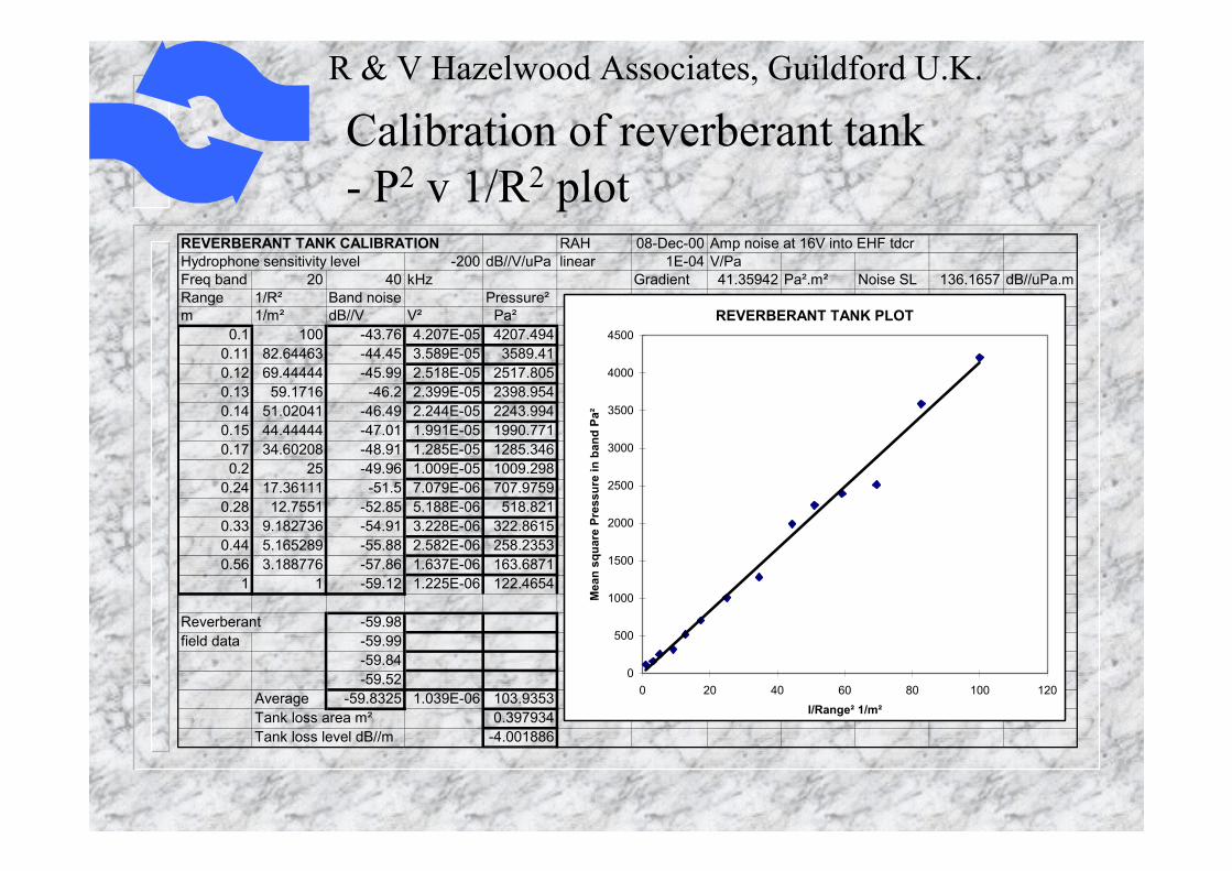
Noise power of underwater machineryNoise power spectra can be measured directly, if the source is

contained within a reverberant environment, such as a test tank. This scheme is analogous to reverberant chamber tests.

Compared with a test offshore, such testing is low cost, and thus useful for design. There is a limit to the spectral resolution and low frequency data, dependent on the tank size, but there is no need to control the precise test geometry

All directional information is lost as the sound echoes around the tank, but this is advantageous if a directional average is required for simplicity or due to a lack of information on operational attitudes.

The tank needs to be calibrated to assess the reverberation.


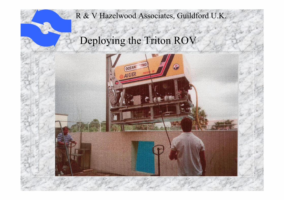
Perry Tritech test tank in Florida - the calibration hydrophone traverse


Deploying the Triton ROV


Calibration of reverberant tank- P2 v 1/R2 plot

REVERBERANT TANK CALIBRATION RAH 08-Dec-00 Amp noise at 16V into EHF tdcrHydrophone sensitivity level -200 dB//V/uPa linear 1E-04 V/PaFreq band 20 40 kHz Gradient 41.35942 Pa².m² Noise SL 136.1657 dB//uPa.mRange 1/R² Band noise Pressure²m 1/m² dB//V V² Pa²

0.1 100 -43.76 4.207E-05 4207.4940.11 82.64463 -44.45 3.589E-05 3589.410.12 69.44444 -45.99 2.518E-05 2517.8050.13 59.1716 -46.2 2.399E-05 2398.9540.14 51.02041 -46.49 2.244E-05 2243.9940.15 44.44444 -47.01 1.991E-05 1990.7710.17 34.60208 -48.91 1.285E-05 1285.3460.2 25 -49.96 1.009E-05 1009.298

0.24 17.36111 -51.5 7.079E-06 707.97590.28 12.7551 -52.85 5.188E-06 518.8210.33 9.182736 -54.91 3.228E-06 322.86150.44 5.165289 -55.88 2.582E-06 258.23530.56 3.188776 -57.86 1.637E-06 163.6871

1 1 -59.12 1.225E-06 122.4654

Reverberant -59.98field data -59.99

-59.84-59.52

Average -59.8325 1.039E-06 103.9353Tank loss area m² 0.397934Tank loss level dB//m -4.001886

REVERBERANT TANK PLOT

0

500

1000

1500

2000

2500

3000

3500

4000

4500

0 20 40 60 80 100 120I/Range² 1/m²

Mea

n sq

uare

Pre

ssur

e in

ban

d Pa

²


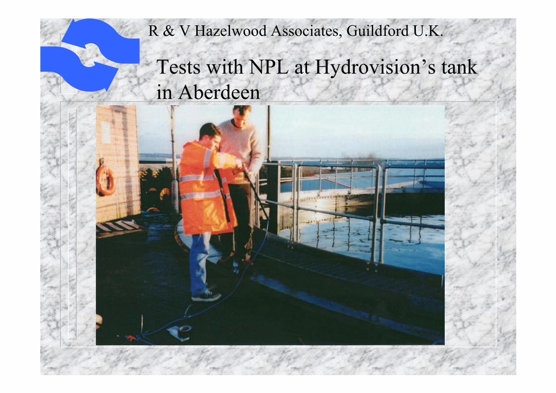
Tests with NPL at Hydrovision’s tank in Aberdeen


The “simple environment”

Reality is seldom simple, but simplification is beneficial, evenat some loss of accuracy, to help to define the “big picture” or to make measurements economically viable.

The “sonar equations” do this by starting with an assumption of a free field with no significant echoes(no reverberation).

In this case the pressure P falls with increasing range r, but the product P·r remains constant.

This gives the sonar equation for source level (SL) asSL = 20 log (P·r ) = 20 log P + 20 log r

For the SL to be independent of range a free field is needed.


Near surface propagation-a limit case

Whilst spherical spreading in a free field provides a way to characterise the source, noise levels at a distance are often raised by reverberation. Test tanks provide extreme conditions but energy can also be confined to a surface layer by a combination of reflection from the surface and refraction within the water, to form a “duct”, of depth H.

This can produce conditions of cylindrical spreading, particularly on a calm night following a mixing of the surface layer to minimise thermal gradients.

In this case the noise pressure level (PL) at range r rises to PL = SL - 10 log r - 5 log H -5 log (11250)equivalent to a constant P² r factor (P ∝ 1/√r)


Propagation by surface duct- isothermal mixed layer

radius of curvature R (typically 90km, not shown to scale)

Duct depth H

Source detail

Surface waves - sea state S

source depth d sound reflected off the surface

sound refracted along circular pathand back to the surface

sound lost into seabed


Near surface propagation-the isothermal duct - a limit case

The propagation law given above has the advantage of being independent of site specific data, and thus useful for project planning, without requiring site surveys.

Although it only provides a limit case, this is still useful in conditions where a conservative estimate is adequate. In critical conditions, more accurate work would be required.

It can usefully be modified to cover conditions where there is significant surface wave scattering, as this does limit the range, or the estimated noise levels, in a predicted way.

When used to cover both the contributions of the planned work, and the estimated background noise, the possible errors in estimated signal/noise ratio are reduced.


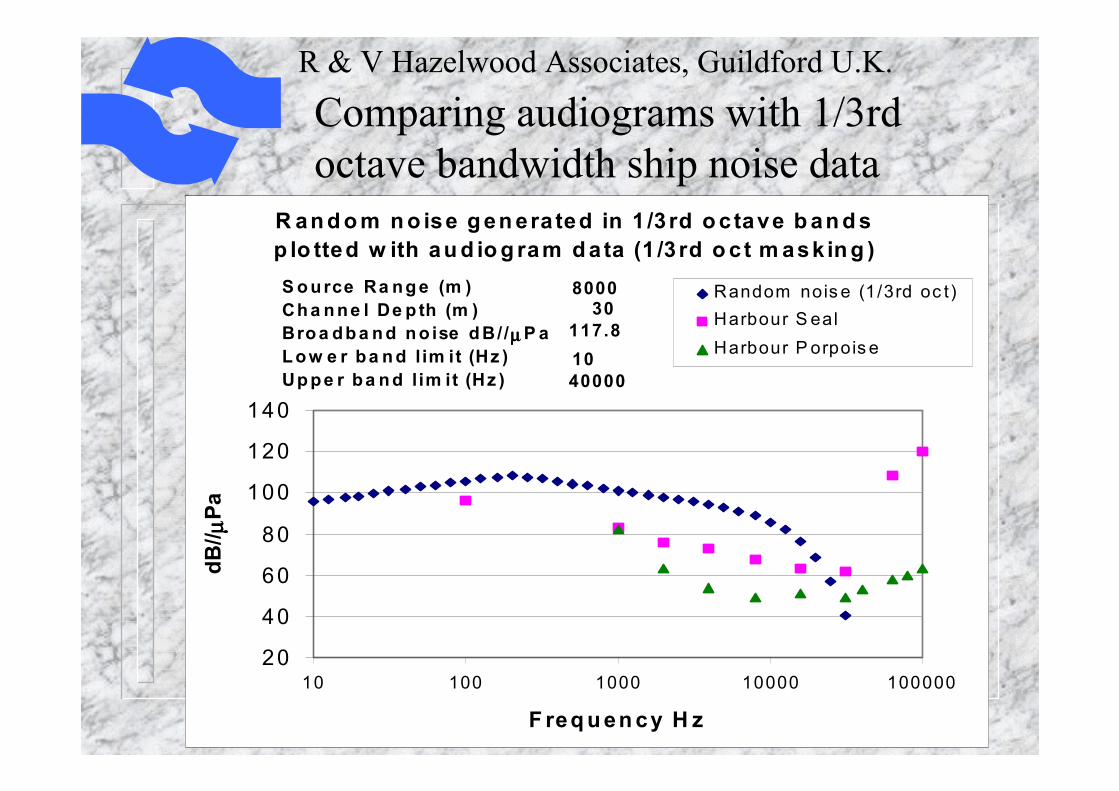
Comparing audiograms with 1/3rd octave bandwidth ship noise data

R an d o m n o ise g en era ted in 1 /3 rd o c tave b an d s p lo tted w ith au d io g ram d ata (1 /3 rd o c t m ask in g )

20

40

60

80

100

120

140

10 100 1000 10000 100000

F req u en cy H z

dB// µµ µµ

Pa

Random nois e (1/3rd oc t)Harbour S ealHarbour P orpois e

S o urce Ra ng e (m ) Ch a n ne l De p th (m ) Bro a db a n d n o ise d B//µµµµ P a L ow e r ba n d l im it (Hz ) Up pe r ba n d l im it (Hz )

800030

1040000

117.8


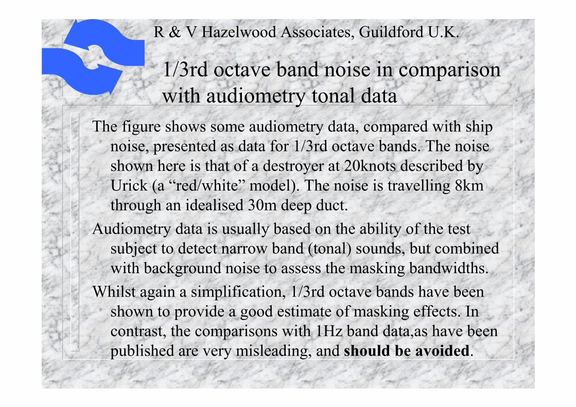
1/3rd octave band noise in comparison with audiometry tonal data

The figure shows some audiometry data, compared with ship noise, presented as data for 1/3rd octave bands. The noise shown here is that of a destroyer at 20knots described by Urick (a “red/white” model). The noise is travelling 8km through an idealised 30m deep duct.

Audiometry data is usually based on the ability of the test subject to detect narrow band (tonal) sounds, but combined with background noise to assess the masking bandwidths.

Whilst again a simplification, 1/3rd octave bands have been shown to provide a good estimate of masking effects. In contrast, the comparisons with 1Hz band data,as have been published are very misleading, and should be avoided.


Summary of simpler estimate schemes

Red/white noise source models can be given in WattsPower leakage can be used to estimate source wattageROV data shares many properties with ship noise.Propagation depends on reverberation but -shallow water limit can be estimated as idealised ductComparison of operational and background noise -uncertainties in propagation are then less criticalComparison of audiometry data with wide band noise -important to integrate noise over masking bandwidths.

AcknowledgementsThe measurements described involved many others including Sonardyne International Ltd Yateley, UK Perry Tritech, Jupiter, USA (Triton ROV)Racal Survey, BP Exploration and BUE Caspian (MV TabrizStolt Comex, Hydrovision and NPL (SCV23 ROV)Nat Oceanographic Centre Southampton UK (ISIS ROV)- thanks to Gwyn Griffiths for permission to publish data. The theoretical work was supported by Metoc plc, UKand assisted by discussion with Royal Haskoning, Nederland. The academic references are given in the paper in Underwater Technology 26,3 2005

R & V Hazelwood Associates LLP,Guildford U.K.

Underwater Noise Measurement SeminarNPL 13th Oct 2005

Date post:	11-May-2018
Category:	Documents
Upload:	hoangtuyen
View:	218 times
Download:	2 times

Estimation of Underwater Noise - a simplified...

Documents