Policy Research Working Paper 7292 Ethiopia’s Growth Acceleration and How to Sustain It Insights from a Cross-Country Regression Model Lars Christian Moller Konstantin M. Wacker Macroeconomics and Fiscal Management Global Practice Group June 2015 WPS7292 Public Disclosure Authorized Public Disclosure Authorized Public Disclosure Authorized Public Disclosure Authorized
Transcript
Policy Research Working Paper 7292
Ethiopia’s Growth Acceleration and How to Sustain It
Insights from a Cross-Country Regression Model
Lars Christian MollerKonstantin M. Wacker
Macroeconomics and Fiscal Management Global Practice GroupJune 2015
WPS7292P
ublic
Dis
clos
ure
Aut
horiz
edP
ublic
Dis
clos
ure
Aut
horiz
edP
ublic
Dis
clos
ure
Aut
horiz
edP
ublic
Dis
clos
ure
Aut
horiz
ed
Produced by the Research Support Team
Abstract
The Policy Research Working Paper Series disseminates the findings of work in progress to encourage the exchange of ideas about development issues. An objective of the series is to get the findings out quickly, even if the presentations are less than fully polished. The papers carry the names of the authors and should be cited accordingly. The findings, interpretations, and conclusions expressed in this paper are entirely those of the authors. They do not necessarily represent the views of the International Bank for Reconstruction and Development/World Bank and its affiliated organizations, or those of the Executive Directors of the World Bank or the governments they represent.
Policy Research Working Paper 7292
This paper is a product of the Macroeconomics and Fiscal Management Global Practice Group. It is part of a larger effort by the World Bank to provide open access to its research and make a contribution to development policy discussions around the world. Policy Research Working Papers are also posted on the Web at http://econ.worldbank.org. The authors may be contacted at [email protected] or [email protected].
Ethiopia has experienced a growth acceleration over the past decade on the back of an economic strategy empha-sizing public infrastructure investment and supported by heterodox macro-financial policies. To analyze the country’s growth performance during 2000–13, the paper employs a neoclassical cross-country System Generalized Method of Moments regression model. The analysis finds that acceler-ated growth was driven by public infrastructure investment and restrained government consumption, and supported by a conducive external environment. Macroeconomic chal-lenges arising from declining private credit, real currency overvaluation, and relatively high inflation held back some
growth. The model accurately predicts Ethiopia’s growth over the period of analysis and is robust to country-specific parameter heterogeneity and alternative infrastructure vari-ables. Looking ahead, model simulations under alternative policy scenarios are indicative that growth may decelerate in the coming decade, making it challenging for Ethiopia to attain its middle-income country target by 2025. Although simulated growth rates do not vary much by policy sce-nario, the paper discusses some of the emerging risks associated with a continued reliance on the current infra-structure financing model and potential future adjustments.
Ethiopia’s Growth Acceleration and How to Sustain It - Insights from a Cross-Country Regression Model
Lars Christian Moller The World Bank Group
Konstantin M. Wacker
The World Bank Group and University of Mainz JEL Classifications: O47, O55 Keywords: Economic growth, determinants of growth, economic growth policy Acknowledgements: This paper contributes to a forthcoming World Bank report on the same topic. The authors would like to thank Mesfin Bezawagaw, Clarie Hollweg, Ashagrie Moges, and Eyasu Tsehaye for helpful support and inputs. Useful comments on previous drafts were received from: Ed Buffie, Kevin Carey, Guang Chen, Pablo Fajnzylber, Maya Eden, Senidu Fanuel, Verena Fritz, Michael Geiger, Fiseha Haile, Ruth Hill, Jan Mikkelsen, Aart Kraay, Pedro Martins, Andrea Richter, Greg Toulmin, and Shahid Yusuf and the participants at the Ethiopia Country Economics Day held at the World Bank. Thanks also to Chris Papageorgiou for making the reform index data set of Prati et al. (2013) available. The paper benefitted considerably from the World Bank project ‘Benchmarking the Determinants of Economic Growth in Latin America and the Caribbean’ (Araujo et al., 2014), funded by the Latin America and Caribbean Office of the Chief Economist as well as the corresponding background work by Brueckner (2013).
1. Introduction
Ethiopia’s development performance over the past decade has been one of the most successful among low-income countries. The country achieved rapid and inclusive economic growth averaging 10.9 percent in 2004-2014 (Figure 1.1), according to official data.1 Substantial progress was made across a broad range of social and human development indicators (World Bank, 2015). Between 2000 and 2011, poverty declined from 44 to 30 percent while income inequality remained unchanged at one of the lowest levels observed worldwide (Gini coefficient: 0.3). Life expectancy increased by one year per year (from 52 to 63 years), fertility declined from 7 to 4 children per woman, and the share of the population without education fell from 70 percent to 50 percent. Ethiopia achieved the Millennium Development Goals on poverty, hunger and child mortality and access to water. Since 2000, the country moved from being the 2nd to the 9th poorest country in the world, according to gross national income (GNI) per capita (Atlas Method). Despite this impressive progress, the country faces deep challenges in every dimension of development. One key challenge is to sustain rapid economic growth. Ethiopia has experienced a growth acceleration since the early 2000s. By taking into consideration population growth of 2.4 percent per year, real GDP per capita increased by 8.3 percent per year between 2004 and 2014.2 This substantially exceeds per capita growth rates achieved in the first decade after the country’s transition to a market-based economy (1992-2003: 1.3%), under the communist Derg regime (1974-91: -1.0%), and during monarchy (1951-73: 1.5%). It has also exceeded regional and low-income averages over the past decade (Figure 1.2). Summers and Pritchett (2014) calculate that annual per capita growth across all countries has averaged 2 percent since 1950 with a standard deviation of 2 percent. Thus, Ethiopia’s recent growth performance has exceeded this global average by more than three times the standard deviation. More generally, this episode falls into the category of ‘growth accelerations’ discussed in the literature by Hausmann et al. (2004), Virmani (2012), and Rodrik (2013).
A first pass at the data highlights the relative importance of productivity growth, capital accumulation, and structural change. While agriculture was the main growth contributor at the beginning of the take-off, the services sector gradually took over in terms of importance and was later complemented by a construction boom (Figure 1.3). In contrast with many other fast-growing African economies, Ethiopia’s growth does not depend on natural resources. Private consumption was important on the demand side, though investment (especially public) has become increasingly important in recent years (Figure 1.4). Solow growth decompositions show that high total factor productivity growth and capital accumulation account for most growth (Figure 1.5). A Shapley decomposition reveals that most of the increase in value added per person arose from higher labor productivity (Figure 1.6). A rising working age population share boosted growth since 2005, but growth was held back by a decline in the employment rate owing to a rising student population. Labor productivity, in turn, increased mainly in agriculture and services, supported by growth-promoting structural change (largely from agriculture into construction and services).
1 The IMF (2013b) has argued that official growth rates may have been overestimated by as much as 3 percentage points in recent years. Even by this more conservative estimate, a growth acceleration was observed. 2 Using UN population estimates and applying them to the official national accounts data of GDP in constant factor prices.
2
Figure 1. Ethiopia: Economic Growth and Contributing Factors 1. Real GDP growth 2. Real GDP growth in Ethiopia, SSA and LICs
3. Real GDP Growth (supply side) 4. Real GDP growth (demand side)
5. Solow Growth Decomposition of Real GDP 6. VA per person growth (% contribution), 2005-13
Note: VA=Value Added. Sources: 1.1-1.2: World Bank (WDI). 1.3-1.4 Staff Estimates based on MOFED data. 1.5: IMF (2013a). 1.6: Martins (2015). SSA5: Burkina Faso, Mozambique. Rwanda, Tanzania, Uganda.
Gov. Cons Priv. ConsTotal Inv. Net ExportGDP Growth
1.70.7
2.4
0.8
1.0
2.10.7
0.4
0.3
-1.1
0.9
3.4
-2
0
2
4
6
8
10
1980-90 1990-2000 2000-10
TFP
Education
Adjusted Labor
Capital
71.656.8
76.2
17.2
8.8
24.55.142.5
-13.7
6.2
-8.0
13.0
-20
0
20
40
60
80
100
120
1999-2013 1999-05 2005-13
Demographic Effect
Employment Rate
Structural change
Within sectorproductivity
3
Ethiopia’s growth experience stands out from a group of similar, high-performing regional peers. Five other non-resource dependent African economies also experienced high growth rates: Burkina Faso, Mozambique, Rwanda, Tanzania, and Uganda (labeled ‘SSA5’). According to the IMF (2013a), these countries (including Ethiopia) share several key characteristics which help explain their growth performance, such as improved macroeconomic management, stronger institutions, increased aid, and higher investment in human and physical capital. This leads the authors to conclude that ‘their experience demonstrates that improvements in macroeconomic policy combined with structural reforms and reliable external financing, can foster productive investment and stimulate growth’ (ibid). A closer inspection of the Ethiopian experience, however, reveals that it fits this narrative only partially. What sets Ethiopia markedly apart is its emphasis on a state-led model of development (which most peers moved away from), the absence of recent structural economic policy reforms, and somewhat inferior macroeconomic outcomes. Ethiopia’s economic strategy emphasizes public infrastructure investment supported by heterodox financing mechanisms. The public investment rate rose from about 5 percent in the early 1990s to 18.6 percent of GDP in 2011, making it the third highest in in the world (World Bank, 2013). Public investment projects are implemented over the national budget and through state-owned enterprises (SOEs) using domestic and external sources of financing. Domestic financing draws on a range heterodox arrangements, including lending and bond purchases by state-owned banks to finance SOE projects and direct budget financing by the National Bank of Ethiopia. The dominance of state-owned banks (accounting for about two-thirds of banking system assets) and credit rationing in the presence of negative real interest rates imply cheap sources of financing for public projects, but also lead to the exclusion of many private investment projects. This partly explains why the private investment rate in Ethiopia is the sixth lowest worldwide (Ibid). Massive infrastructure investments are taking place in the energy, transport, communications, agriculture and social sectors, albeit from very low levels. Power generation capacity increased from 473 MW in 2002 to 2,268 MW in 2014, and is projected to reach 4,138 MW by 2015. More than 10,000 MW generation capacity will be available by 2020 once major ongoing hydro, geothermal and wind projects have been completed. Chief amongst these is the construction of Africa’s largest dam, the Grand Ethiopian Renaissance Dam at a cost of US$4.2 billion (8.5 percent of GDP). The federal and regional road network increased from 26,500 km in 1997 to 60,000 km in 2014. Railway lines connecting Addis Ababa with the Port of Djibouti as well as a Light Railway line in the capital are near completion. The customer base of Ethio Telecom (a state monopoly) rose from 7 to 26 million (mobile, fixed, internet) in 2011-14 and projects to upgrade the existing networks are ongoing. On the other hand, the pace of structural economic policy reform has been relatively slow in Ethiopia, especially in recent years. There is a growing consensus that both macro- and microeconomic policy reforms can lead to improvements in resource allocation, productivity, and growth (Dabla-Noris et al., 2014). Between 1991 and 2003, as it was transitioning away from communism, Ethiopia implemented wide-ranging market-oriented reforms, but achieved relatively modest economic growth. Conversely, during the growth acceleration period between 2004 and 2014 major structural policy reforms were largely absent. Arguably, the economy would not have taken off in the second period without the reforms of the first period suggesting that these were a necessary condition for growth and that their positive impact was lagged. At the same time,
4
concurrent economic reforms could not have been a major driver of the growth acceleration precisely because the reform effort slowed down in this period. Annex Figure A.1 illustrates the slow pace of structural economic policy reform in Ethiopia in the early 2000s in contrast with the five regional peers (SSA5) using the index developed by Prati et al. (2014) for reforms in six reform areas (agriculture, domestic finance, trade, capital accounts, networks, and current account). The motivation for this paper is to contribute to a systematic and rigorous explanation of Ethiopia’s growth acceleration and to identify critical factors to sustain it. Apart from regional or sub-regional studies, including IMF (2013a), Ethiopia’s growth acceleration has not achieved much attention in the literature.3 Our paper, and the report to which it contributes, seeks to fill this gap by addressing two key questions: What explains Ethiopia’s growth acceleration since 2004? And which growth policies offer Ethiopia the best opportunity of sustaining high growth to attain middle-income status? To address them, we employ a cross-country System Generalized Method of Moments (GMM) regression model developed by Brueckner (2013).4 This approach facilitates a systematic classification of growth drivers into three broad categories: structural factors, stabilization policies, and external conditions.
Our key findings are summarized as follows: Overall, the model provides good predictions of Ethiopia’s growth performance since 2000 and our results offer plausible quantitative explanations for key economic trends and policy developments over this period. We find evidence that public infrastructure investment ‒ financed in part by restrained government consumption ‒ was the key structural driver of growth. While this policy mix enjoys broad support among mainstream macroeconomists, heterodox policies pursued by the Ethiopian government such as financial repression, an overvalued real exchange rate, and monetary policy induced inflation (including ‘printing money’ to finance public spending) are more controversial. Interestingly, the empirical results show that the growth dividend of the former set of policies outweighed the drag from the latter. This helps shed light on the question of how Ethiopia could achieve high economic growth in the presence of seemingly growth-inhibiting macro-financial policies. Looking ahead, model simulations under alternative policy scenarios are indicative that growth is likely to decelerate in the coming decade making it challenging for Ethiopia to attain its middle-income country target by 2025. Although simulated growth rates do not vary much by policy scenario, we discuss some of the emerging risks associated with a continued reliance on the current infrastructure financing model and potential future adjustments. The remainder of this paper is structured as follows: Section 2 outlines the methodology. Section 3 uses model results to explain Ethiopia’s recent growth performance distinguishing between structural, stabilization, and external factors. Section 4 examines model accuracy and robustness. Section 5 uses benchmarking to examine which individual policies would have the highest growth payoff. Section 6 simulates alternative policy scenarios and assess their implications for future growth. Section 7 discusses the results. Section 8 concludes.
3 Aside from the background papers prepared for a forthcoming World Bank report on the same topic by Dogo and Merotto (2014), Ghani and O’Connell (2014), Kray and Eden (2014ab), Martins (2014; 2015), and Yusuf (2014). 4 The System GMM method has been used in cross-country growth studies for the past 15 years. See Bazzi and Clemens (2013) for references to some of the leading applications and a critical discussion.
5
2. Methodology Our analysis is based on previous studies investigating the determinants of growth in developing countries. We use an empirical growth model originally set up by Loayza et al. (2005) which was improved and updated by Brueckner (2013). These cross-country growth regression models were originally constructed to investigate growth in Latin America and the Caribbean (Araujo et al, 2014). Such cross-country growth regressions may have their limitations, but their insights should not be neglected. We are well aware that cross-country growth regressions have their limitations. While some strands in the literature neglect them altogether, we at least view them as one possible approach to gain insights into the dynamics of growth (see also Durlauf, 2009), especially in a country like Ethiopia where data coverage is relatively scarce. Furthermore, our econometric approach tries to address the most conventional methodological issues that can arise in cross-country growth regression exercises. This approach avoids tweaked Ethiopia-specific results. Taking an existing cross-country regression model to analyze Ethiopia’s recent growth performance potentially runs the risk that Ethiopia-specific factors might not be well-reflected in the model. However, this is essentially our goal as setting up a new cross-country model for our purpose will be prone to model selection that produces the ‘best’ results for the specific case of Ethiopia. In essence, our approach helps address the following question: can we explain Ethiopia’s recent growth performance by factors also observed to influence growth in other countries? Or is the Ethiopian case a specific one? Even if one remains skeptical of cross-country growth regressions, a failure of the model to appropriately predict observed growth in Ethiopia would suggests that factors that correlate with growth in most countries cannot explain Ethiopia’s growth acceleration. On the other hand, a good predictive performance would imply that Ethiopia’s growth acceleration is in line with experiences of other countries and allow us to decompose those correlates of growth in more detail. 2.1 Model and Data The underlying model expresses domestic income as function of key growth drivers. Our goal is to estimate the impact of certain variables Xct on domestic income, measured as the natural log of real PPP GDP per capita (lnyct for country c in period t). More formally, the estimated equation can be written as the dynamic (‘steady-state’) process:
lnyct = θlnyct-1 + Γln(X)ct + ac + bt + ect (1)
where ac and bt are country and time fixed effects, respectively; and ect is an error term that remains unexplained by the model (‘residual’, i.e. the difference between predicted and observed growth). Note that a time period t is the average over (non-overlapping) 5-year periods to smoothen short-run and cyclical effects. These drivers of growth are grouped into the categories of structural, stabilization, and external effects. Following the above-mentioned studies, the individual variables in the vector Xct are assigned to those three categories. This facilitates an interpretation whether growth was driven by
6
“good policies” (structural, stabilization) or “good luck” (external). We briefly discuss the individual variables (which are taken from the Brueckner (2013) dataset) and their intuition below. A more detailed technical description, including the original data sources is presented in Annex Table A.1. Stabilization variables contain inflation, banking crises and the exchange rate. Capturing the idea that macroeconomic fluctuations can influence growth over an extended period, we control for the number of banking crises in each period, the inflation rate, and the exchange rate. A decrease in the latter variable is equivalent to a currency depreciation.5
Structural variables capture a broad set of fundamental country characteristics. This includes secondary school enrollment as a proxy for human capital, a measure for trade openness (trade-to-GDP ratio adjusted for population), an institutional variable (polity2), and private credit-to-GDP as a measure of financial development. Our baseline variable for infrastructure is fixed telephone lines per capita but given the substantial impact obtained for this variable, we also perform alternative specifications with mobile phone and road coverage. Furthermore, our model includes government size (government consumption to GDP). Although several government expenditures can have a beneficial effect on income (especially in areas like health, education, or public infrastructure), the essential idea of this variable is to capture the negative effects that an excessive government and associated taxes can have on private activity. As our model describes long run growth, this should not be confused with the positive stimulative effects that increased government consumption can have during economic downturns. It should also be noted that our model is conditional on other variables, i.e. the positive effect of government spending for education and infrastructure, e.g., will be captured by those variables (and lagged GDP).6 Finally, a high level of consumption (i.e. recurrent) expenditures limits fiscal space to counter cyclical shocks. Generally welcome counter-cyclical measures can then only be financed with relatively distortionary taxes (see also Afonso and Furceri, 2010, on the effect of expenditure volatility) or an increased debt burden.7
External factors are reflected in terms of trade and commodity prices. Net barter terms of trade and the country-specific commodity export price index of Arezki and Brueckner (2012) are used to capture the most important effects of the global environment on growth. Furthermore, global conditions will also be reflected in the time dummies.
Although our variables are not perfect, they allow for a large coverage of developing countries. In the best case, one would have more sophisticated variables to reflect the underlying economic
5 As the interpretation of the exchange rate variable is somewhat difficult in the cross-country context from a policy perspective, it should rather be seen as a control variable, i.e. controlling for the fact that an undervalued exchange rate might boost growth temporarily. 6 See also Loayza et al. (2005: 40-41). Optimally, one would like to subtract such expenditures like health, education, or infrastructure but this is not feasible for the wide range of countries included in the sample. Following the line of reasoning above, one should also note that the negative effect of government size is considerably smaller when the model is estimated unconditionally (i.e. without controlling for other variables), reflecting the fact that it then implicitly captures the positive effects of education, infrastructure etc. (see the results in Araujo et al., 2014, especially Tables 3 and A.3). 7 For an alternative view on the effects of government consumption on output in neoclassical growth models, see e.g. Aiyagari et al. (1992) and the literature therein.
7
rationale. For example, educational achievements might be a better proxy for human capital than attainments. Unfortunately, data on such a level of quality is not available for a broad range of countries. Researchers thus face a trade-off between data sophistication and country coverage. Since data quality is especially poor in lower income countries, while our goal is to include them in the sample to obtain most appropriate estimates for Ethiopia, we are thus limited to the mentioned data at hand. On the upside, this leaves us with a panel of 126 countries for the 1970-2010 period (see Annex Table A.3 for country coverage). 2.2 Estimation We use System GMM estimation with a limited set of internal instruments. This method is appropriate as some of the explanatory variables, Xct, may themselves be a function of the dependent variable and because dynamic panel estimation in the presence of country fixed effects generally yields biased estimates (e.g. Nickel, 1981; Wooldridge, 2002). Our estimator uses internal instruments to avoid endogeneity biases. More specifically we use one first-differenced lag of the explanatory variables as instrument for those variables in levels which is valid under some assumptions (see Arellano and Bover, 1995, and Blundell and Bond, 1998).8 Our estimation strategy addresses most conventional methodological pitfalls. The inclusion of country fixed effects avoids unobserved heterogeneity across countries while the use of internal instruments avoids endogeneity biases. By limiting the instrument set to one lag we avoid the well-known problems associated with too many instruments (Roodman, 2009). Since the outset of the Brueckner (2013) study, recent findings have shown that this might give rise to the opposite problem of suspiciously weak instruments (Bazzi and Clemens, 2013; Kraay, in progress) which we briefly address in the robustness section.
Our econometric model is considered most appropriate to estimate neoclassical growth models over a policy-relevant horizon and has been tested for robustness on several fronts. Despite the limitations and concerns about System GMM, we find it to be the most appropriate estimation method for our purpose as it can incorporate a wide range of (linear) relationships among current and lagged values of economic variables, helps isolate exogenous changes in a variable from automatic reactions of that variable to other variables in the system and is careful to not confuse the change in a variable with a temporary shock. Furthermore, the identification strategy over time variation makes it appropriate to assess our periods of interest for one country, as opposed to identification strategies using cross-country variation (like the between-effects estimator) that also potentially suffer from unobserved cross-country heterogeneity. Given the dimension of our panel data set (especially the focus on a relatively short period) and some data gaps, we also find it superior to cointegration methods. To address remaining concerns, we also perform several
8 We limit the instrument set to one lag in the baseline model in order to ensure that the number of instruments does not grow too large in the System GMM estimation and furthermore avoid over-fitting the model by using the ‘collapse’ sub-option in the STATA xtabond2 command. Commodity prices, terms of trade and time dummies are treated as exogenous. We also use the one-step estimator as the two-step estimator is infeasible given the dimension of our data set. This also avoids severely downward biased standard errors associated with the two-step estimator (Blundell and Bond, 1998). See Brueckner (2013) for further details and discussions.
8
robustness checks in addition to the battery of checks applied by Brueckner (2013), as discussed in Section 4. 2.3 Calculating Growth Contributions in Ethiopia Growth contributions over each time period can be calculated by first-differencing equation (1):
Δlnyct = θ(Δ lnyct-1)+ ΓΔln(X)ct + Δbt + Δect (2)
as log-changes approximate growth rates of a variable. I.e. growth can be explained by a persistence effect (θ[Δ lnyct-1]), changes in the explanatory variables X, and a period-specific global shock (Δbt).9 Note that the country fixed effect cancels out because it is time-invariant. To illustrate: growth in the Late 2000s can be explained by a dynamic persistence effect from the Early 2000s, the change in explanatory variables X in the Late 2000s, and a global time-specific shock (relative to the previous period). In this setting, the persistence effect should be interpreted as an ‘echo’ (or fading out) of previous improvements. Finally, the residual part Δect remains unexplained by the model. For calculating Ethiopia's drivers of growth, we extend its explanatory variables by one 5-year period. As the original dataset by Brueckner (2013) contains average 5-year values across countries until 2010 only, we update the Ethiopia values using 2013 data. We treat the latter period (the ‘Early 2010s’) as if it represented a 5-year period average for 2011-2015. This can be motivated by the consideration that the 2013 value is the mid-point for this period and most macro variables are highly persistent. Since not all of the 2013 data were available from sources fully consistent with the original dataset we added to the logged original series the log changes between the 2006-2010 averages and the 2013 values of those data we had available.10 Despite some caveats, this approach allows us to also analyze the most recent period of Ethiopia’s growth performance. Furthermore, it should be noted that this extension does not affect the model estimation results as it was performed after estimation for Ethiopia only.
To facilitate an analysis of the growth acceleration period since 2004 with the available data, it is useful to define time periods precisely. As illustrated in Figure 2, our analyzed period 1996-2013 consists of 4 data points (t0, t1, t2 and t3), each capturing the average values of the following time periods: 1996-2000, 2001-2005, 2006-2010, and 2011-2015 (proxied by the 2013 value). In the remainder of the paper, we refer to ‘Early 2000s’ as the change between the 1996-2000 and 2001-
9 Our calculation differs slightly from the one in Brueckner (2013) and Araujo et al. (2014) as we do not use the actual lag of the growth rate for calculating the persistence effect from equation (2) but instead take the growth rate as predicted from the model. Furthermore, we take second differences of external factors as they enter the estimated levels equation already in first differences. To calculate effects for the 2000-2013 period, we proceed as follows to accommodate dynamic effects: we calculate the changes over the full 15-year period and multiply them by the respective coefficient Γ times (3+2θ+θ2)/3. This assumes that the change has been uniform over time and accommodates their dynamic effects. Similarly, the persistence effect is calculated as (θ+ θ2+ θ3)/3 times the growth rate in the period prior to 2000. 10 Where series were not identical (e.g. education), adding log (i.e. percentage) changes still provides a good proxy. For the commodity price index growth, we decided to take the 90th percentile of previous index changes in Ethiopia. This was fairly consistent with our attempts to construct a similar index for this period. For the real exchange rate, we used IMF data for the Real Effective Exchange Rate (using the fiscal year 2013/14 as reference) as a proxy.
9
2005 averages, the ‘Late 2000s’ is defined as the performance between the 2001-05 and 2006-10 averages, and the ‘Early 2010s’ comparing 2006-2010 averages and 2013 values.
Figure 2: Definition of time periods used in the study 1996 2000 2005 2010 2013
Avg. 1996-2000 Avg. 2001-2005 Avg. 2006-2010 2013 t0 t1 t2 t3 Early 2000s Late 2000s Early 2010s
2000-2013
It is also instructive to recap the implications and dynamics of this empirical neoclassical growth model. Levels equation (1) implies that the (log) level of GDP changes with the (log) level of the explanatory variables X. Any change or innovation in the (log) level of X will thus have a permanent effect on (log) GDP and the effect is intermediated through a temporary (transitory) effect on the growth rate. A one-time increase in human capital in the Early 2000s, for example, will thus be captured as Δln(x) > 0 in equation (2) and impact the growth rate in the same period with parameter Γ. This growth-enhancing effect will be echoed in the Late 2000s via the lagged dependent variable effect as θ Γ < Γ (which is captured as persistence effect in our model) and eventually fade out over time. 3. Explaining Ethiopia’s Recent Growth Performance Our model is well specified and consistent with economic theory. Results are presented in Tables 1, 2 and Figure 3. Column 1 in Table 1 shows the baseline results of the model estimation, while columns 2-4 summarize robustness checks discussed in Section 4. Table 2 illustrates the baseline results for Ethiopian data for the four time periods (2010-13, Early 2000s, Late 2000s, and Early 2010s). Overall, there is no indication that the model is mis-specified and parameters show the expected signs, except from the institutional variable Policy2 which is statistically insignificant.11 Parameter estimates are either statistically significant or at the borderline of significance, except for schooling which is a well-known issue in growth regressions (e.g. Pritchett, 2001) and should not lead to neglect of education policies. Figure 3 illustrates the more detailed results of Table 2.
11 Institutional quality usually does not vary as much over time, so it is difficult to identify the according parameter in this context.
as FE No of instruments 153 166 171 AB(1) 0.023 0.024 0.033 AB(2) 0.102 0.045 0.062 Sargan test 0.131 0.017 0.001
Note: Based on Brueckner (2013). Standard errors in parentheses. ***, **, and * indicate statistical significance on the 1, 5, and 10 percent level, respectively. AB(1) and AB(2) is the p-value of the Arellano and Bond test for first
and second order autocorrelation, respectively. Sargan test reports p-values.
11
Table 2: Parameter values, changes and predicted growth effects (real GDP per capita). 2000-13 Early 2000s Late 2000s Early 2010s
Source: Authors’ calculation, obtained by inserting Ethiopian values for the explanatory variables and using the regression coefficients of the baseline model presented in Table 1 (column 1).
12
Figure 3: Regression results: Key Growth Drivers in Ethiopia (Real GDP per Capita).
Source: Table 2.
Economic growth in 2000-13 was driven primarily by structural improvements, according to model results. The left panel of Figure 3 shows that almost all of the (predicted) growth performance of the 2000-2013 period can be attributed to structural factors: the model estimates these factors to have contributed 3.8 percentage points (ppts) of average annual per capita growth rate of 4.2 percent. The positive effect of the external environment was outweighed by the negative effects associated with macroeconomic imbalances (each accounting for 0.3 ppts). The remaining growth impetus was explained by persistence effects. Public infrastructure investment and restrained government consumption were the key structural drivers of growth. These two factors were linked as an expansion in budgetary infrastructure investment was facilitated by reduced government consumption, arising partly as a result of a ‘peace dividend’ effect following the end of the 1998-2000 war with Eritrea (Figure 4.2). As previously mentioned, public investment was also financed by extension of credit through the domestic banking sector and foreign borrowing and partly executed through off-budget state owned enterprises. It also helped for growth (0.2 ppts) when Ethiopia opened more to international trade, especially in the Early 2000s, as trade of goods and services increased its share of GDP from 37.5 percent in 2002 to 48.7 percent in 2012 (World Bank, 2014a).12 Although Ethiopia made substantial efforts in improving educational attainment of its population over the past decade, the growth enhancing effects hereof have been somewhat modest (0.3 ppts), as reflected in the regression results and the Solow decomposition results presented earlier (Figure 1.5), though this may be a measurement problem as discussed by Pritchett (2001). Secondary education (the explanatory variable) remains limited, even if gross enrolment improved from 13.1 to 32.8 percent over the period of analysis.13
12 See also Figure A1 on the trade policy reform side. 13 See World Bank (2012) for an analysis of the challenges related to secondary education in Ethiopia. There is also evidence of a substantial mismatch between skills supply and demand, for instance in manufacturing (World Bank, 2014b).
Financial disintermediation held back some growth. An expansion of credit to the private sector enables firms to invest in productive capacity, thereby laying the foundation for a sustainable growth path. However, Ethiopia is falling behind its peers in this area (Figure 4.3). Regression results suggest a small negative growth effect of financial repression policies whereby rationed credit is channeled through state-owned banks primarily towards public investment (see Figure 7.2). It is noteworthy that the negative quantitative effect was substantially smaller than what is generally perceived (-0.2 ppts in 2000-13). On the other hand, the growth penalty shows an increasing trend (rising to -0.3 ppts in the Early 2010s), suggesting that financial repression policies may become more costly if maintained. Indeed, this would be consistent with the experience of China.14 Structural improvements were particularly important in the late 2000s supported by a positive external environment, but held back by macro imbalances. How did growth drivers change over time? While structural factors dominate in the Early 2000s (2.5 ppts) and Late 2000s (3.0 ppts), they become less pronounced in the Early 2010s (1.2 ppts). The diminishing effect in the last period, however, is affected by the choice of the infrastructure variable, as discussed in Section 4. The growth contribution of the external environment increased over the period, shifting from a negative (-0.6 ppts) to a positive contribution (1.0 ppts) between the Early 2000s to the Late 2000s and a weak positive effect in the Early 2010s (0.2 ppts). The deteriorating macro environment was a drag on growth only during the late 2000s (-0.6 ppts), but not in the other two periods. The substantial persistence effect observed in the late 2000s and early 2010s (about 3 ppts) echoes the growth drivers during the early and late 2000s, respectively. We interpret this as the lagged effect of the structural improvements implemented in earlier periods.15 An improved external environment supported the growth acceleration. As argued in World Bank (2014a), a strong rise in exports helped support the economic boom. Since 2003 exports quadrupled in nominal terms, while volumes doubled, reflecting a substantial positive price effect (Figure 4.4). This is consistent with findings by Allaro (2012) that exports ‘Granger caused’ growth. The strong growth effect is somewhat surprising and may be an over-estimate given that merchandise exports account for only 7 percent of GDP – the lowest among populous developing countries (services exports account for an additional 7 percent of GDP). The growth drag of macroeconomic imbalances sets Ethiopia apart from high performing regional peers, though the effect was modest. Growth was held back by high inflation and an overvalued exchange rate in the Late 2000s. The country experienced much larger inflationary impacts of the two commodity price shocks in 2008 and 2011 than other low-income and African countries (Figure 4.5). This is partly explained by expansionary policies in the form of high growth of the monetary base owing to credit expansions to state owned enterprises and direct central bank lending to the government. Following the 2010 devaluation, the monetary authorities also allowed the unsterilized accumulation of foreign exchange reserves arising from the ensuing rise in exports and this contributed to additional inflation (inducing a growth penalty of 0.3 ppts in the Late 2000s). Most other countries in Africa achieved better monetary control by shifting toward reliance on indirect instruments like open market operations to soak up liquidity. Monetary policy
14 See Huang and Wang (2011) for a review of the effects of financial repression policies on growth and for empirical evidence suggesting that such policies were conducive in the early (but not later) stages of growth in China. 15 The subsistence effect should not be conflated with the unexplained residual as per Equation (2).
14
Figure 4: Trends in Key Growth Drivers 1. Infrastructure Trends 2. Public investment and consumption (% of GDP)
3. Private sector credit (% of GDP) 4. Exports: Value and Volume, 2000-2011
instruments in Ethiopia, in contrast, are limited to changes in bank reserve requirement and sales/purchases of foreign exchange reserves. In addition, the real exchange rate was allowed to appreciate substantially since 200416, owing to insufficient nominal depreciation in a system of foreign exchange rationing (Figure 4.6).17 This made the import of expensive public infrastructure equipment relatively cheaper but undermined export competitiveness. The net effect on growth was negative (0.3 ppts in the Late 2000s), though not as substantial as estimated elsewhere. Nevertheless, what stands out from these simulations is that the growth penalty of somewhat less optimal macro policies was not that substantial. High inflation and an overvalued exchange rate cut little over half a percentage point from economic growth rates. This helps explain why Ethiopia was able to grow fast in the presence of some sub-optimal macro policy choices. Would economic growth have been higher in the absence of heterodox macroeconomic policies? It is hard to give a precise answer to this question. However, it should be pointed out that financial repression, a strong real exchange rate and monetary policy induced inflation all helped support high public infrastructure investment. By providing full access to credit at negative real rates and foreign exchange at below market prices, the cost of public investment was reduced substantially. Moreover, direct central bank financing of the budget deficit and seignorage allowed more public investment to be financed, thus supporting growth. In the presence of more orthodox macro policies, public infrastructure investment would have been lower, which would have lowered growth. The net growth effect of these two alternatives is difficult to estimate with precision, but it is unlikely that that public infrastructure investment could be maintained at similar high levels on the back of orthodox macro policies. Several other growth drivers, not identified by the model, are also worth consideration. While the model results discussed above are insightful and plausible they, of course, also have some limitations. Ethiopia’s growth was not exclusively driven by public infrastructure investments, restrained government consumption and favorable terms of trade. As discussed in Section 1, productivity growth, factor accumulation, and structural change were also important drivers. Although some productivity gains were infrastructure related, important advances in agricultural productivity arose from improved farming practices and input use, especially fertilizer (World Bank, 2015). Private investment, albeit low, also contributed to capital accumulation. Finally, shifts of labor out of low productivity agriculture and into higher productivity construction and services activities boosted growth.
16 The degree of real exchange rate overvaluation fluctuated over time. World Bank (2013) shows that the real exchange rate of Ethiopia has remained overvalued throughout the 1951-2011 period. By 2011, the RER over-valuation was 31 percent. The IMF (2014), using alternative methods and measurement, finds that the real effective exchange rate was overvalued by 10-13 percent in 2014. 17 The de facto exchange rate arrangement is classified as a crawl-like arrangement by the IMF (2013b). The authorities describe it as a managed float with no predetermined path for the exchange rate. The annual pace of nominal depreciation, however, has been stable at 5 percent in recent years. The NBE continues to supply foreign exchange to the interbank market based on plans prepared at the beginning of the fiscal year, which take into account estimates of supply and demand.
16
4. Model Accuracy and Robustness Our growth predictions are quite similar to observed rates and the model has a better predictive power than similar studies on Ethiopia. Figure 5 compares actually observed per capita growth with the predictions from the model. As illustrated, the model slightly under-predicts growth in the entire period (2000-2013) while almost perfectly capturing the differing magnitude of the slow growth period in the Early 2000s and the growth acceleration of the Late 2000s. Predictions for the Early 2010s are the least precise, but this can be corrected by a substitution of infrastructure variables, as discussed later. While discrepancies for country-specific results derived from cross-country studies are not exceptional in the literature (see results for LAC countries in Araujo et al., 2014), our residual compares very favorably to the Ethiopia results derived from the cross-country OLS regression model reported in IMF (2013a), where the residual effect predominates. Our residuals are quite small as depicted previously in Figure 3 (gray bars).
Figure 5: Prediction performance of the model
Note: ‘predicted’ is based on the baseline model, ‘predicted alternative infrastructure’ subtracts the effect of phone lines from the baseline result and instead adds the average effect of roads and cell phones. Source: Authors' calculation. Our model passed a series of robustness checks. The original model of Brueckner (2013) also underwent a series of standard robustness checks. For example, it was shown that instrument strength is strong in the GMM regression (by testing the relevant first-stage relationship), that main results are robust to taking 10-year non-overlapping panel data, balanced panel data, time-varying coefficients, or alternative specifications. Furthermore, unconditional models were estimated variable by variable as this limits the weak-instrument problem in the case where various instruments appear strong in isolation but are highly correlated so that they are weak when used together (see Dollar and Kraay, 2003). Further to these results, we present three other
01
23
45
67
89
2000-2013
01
23
45
67
89
Early 2000s
01
23
45
67
89
Late 2000s
01
23
45
67
89
Early 2010s
actual predicted predicted alternative infrastructure
17
specifications in Table 1: column (2) reports the results without the Polity2 variable that had a counter-intuitive sign in the baseline specification. The results (which also allow to include a wider set of countries for which Polity2 is not available) are almost identical to the baseline model in column (1). In column (3) we expand the instrument set for the explanatory variables to include lagged differences for lags 1, 2, and 3 (as opposed to including only the first lag). While not a fully sophisticated check for instrument robustness, this should still convince the reader of the robustness of the results to the used instrument set and that we do not use too few instruments. Results are again similar to the baseline, though the infrastructure parameter is (statistically significantly) smaller but still significant and large. The results of the Sargan test also indicate that the instrument set is not as appropriate as in the baseline model. In column (4) we also report fixed-effect results for comparison, again with similar results to the baseline but a somewhat smaller (but positive and significant) infrastructure parameter. The fact that the lagged dependent variable parameter of this model is somewhat smaller than in the baseline also confirms that our baseline model is well-specified because of the downward bias of this parameter in fixed effect estimation (Nickell, 1981). We also examine whether some variables had a significantly different effect on growth in Ethiopia, but find no substantial Ethiopia-specific effects for growth drivers. As a robustness check, we estimate an Ethiopia-specific coefficient – parameter by parameter. This stepwise procedure is chosen to keep the instrument set in the GMM framework at a reasonable size. Our results do not show any statistically significant deviation of Ethiopia’s determinants of growth from the overall sample of countries included (Annex Table A.5). This is consistent with the findings of Brueckner (2013) that the underlying model is largely robust to parameter heterogeneity. We only find a strong and positive country-specific effect of Polity2 but as this variable is trending upwards in Ethiopia between 1970 and 2000, it only captures the growth of income over time: after controlling for a country-specific time-trend, this Ethiopia-specific variable is no longer statistically significant. Moreover, we exclude Ethiopia from the baseline model to avoid the possibility that Ethiopia itself is driving the results, in which case the good performance of the model to explain the country’s growth would be tautological. Although the broad country coverage of our sample makes this unlikely, the results of Warner (2014) warrant some caution. The results reported in column (2) of Annex Table A.2 however, confirm that the exclusion of Ethiopia from the sample has almost no effect. Some effects differ in lower income countries but these differences are not significant. As one may argue that the overall model includes several high-income countries and is thus not appropriate for Ethiopia, we re-estimate the model using only countries that were below the median or mean of GDP p.c. in 1995. Results are depicted in columns (3) and (4), respectively, of Table A.2 in Annex A. For the (smaller) set of countries initially below the median GDP p.c., there are some parameter differences. E.g. the effects of the exchange rate and of credit/GDP seem somewhat larger. But if we statistically test whether these parameters are significantly different from those obtained in the baseline model (column 1 of Table A.2), we cannot reject the hypothesis that these parameters are equal to those in the baseline model. The effect of telephone lines, on the other hand, seems somewhat smaller. In this case, we can reject the null hypothesis of a parameter equal to the baseline model on the 10 percent (but not on the 5 percent) level of statistical significance. In column (5) of Table A.2 we also re-estimate the model for Sub-Saharan African countries only. Although this dramatically decreases the sample size, results are in line with our
18
baseline model, again with a somewhat smaller infrastructure parameter (that is now only at the borderline of statistical significance). Overall, this provides some weak evidence that our benchmark model somewhat overestimates the positive impact of infrastructure (as proxied by telephone lines).18 Overall, these results support the baseline model but suggest that the infrastructure results may be on the higher side. As demonstrated, our model is robust to a wide range of alternative specifications. Where results differ in magnitude, this difference is rarely statistically significant and thus often reflects random sample effects. The only case where infrastructure is statistically insignificant arises in a considerably reduced sample and the quantitative result is still in line with parameter estimates from other robustness checks. In total, these robustness checks suggest, however, that our estimate for infrastructure in the baseline model may be on the higher side. However, we find no evidence that any of these alternative models would be more appropriate to capture growth in Ethiopia over the recent past. Moreover, even if we assume one of the lower parameter values (which themselves might be on the lower side), the associated contribution of infrastructure to Ethiopia’s growth acceleration would still be substantial and in the range of one percentage point per year. The results are also robust to the choice of alternative infrastructure variables, apart from diverging trends in Early 2010. Given the critical explanatory importance of infrastructure and the difficulty of appropriate measurement and interpretation, we also tested whether results are sensitive to alternative variable specification. The model results reported in Table 1 use fixed telephone line coverage. We tested two alternative infrastructure variables, namely mobile phone subscribers and road coverage and found nearly identical results up to 2010.19 We note that all three types of infrastructure are provided exclusively by the public sector in the case of Ethiopia giving us greater confidence in drawing inferences between public infrastructure investment and growth. Both alternative infrastructure variables have a strong positive impact on growth in our model, although the effect of roads is only at the borderline of statistical significance (z statistic 1.55). The results are depicted in Figure 7.1 as annualized contributions to the overall predicted growth rate (in percentage points). The bars for telephone lines simply reproduces the results depicted in Table 1 to facilitate comparison. We can further see that the effect of fixed telephone coverage and roads for explaining growth in Ethiopia in 2000-13 is nearly identical, despite minor differences in magnitudes and with respect to the timing across sub-periods.20 Differences only arise in the last period (the Early 2010s), which is then also reflected in the 2000-2013 predictions. Over this period, fixed telephone lines were declining but this does not adequately capture infrastructure developments, as some substitution towards cell phones took place and other infrastructure—such as roads—was increasing considerably as well (see Figure 4.1). When correcting for alternative measurements, we are able to predict growth in Early 2010s with greater accuracy. To assess the impact of these alternative infrastructure measures on the overall
18 We also estimated the model for landlocked countries only but due to the small sample size (25 countries with a total of 85 observations), results were mostly insignificant and thus not very informative. See column (6) of Annex Table A.2. 19 As our original data set only covered roads data until 2007 in Ethiopia, we replaced this data using national sources. 20 For a firm-level analysis showing the positive effect of road infrastructure on firm location choice and startup size in Ethiopia, see Shiferaw et al. (2013).
19
predicted growth rate, we subtract the effect of phone lines from our baseline predictions and instead add the average effect of roads and cell phones, with the results depicted in the light-red bar of Figure 5 (‘predicted alternative infrastructure’).21 As one can see, this corrects for this Early-2010s specific effect. Especially if one assumes an average of our baseline prediction and the one with alternative infrastructure, our predictions come very close to the actually observed growth rate. Infrastructure improvements in the early 2010s paid off during later years as well. As one can see from Figure 4.1, our baseline variable of telephone lines saw a considerable pickup (from very low levels) in the Early 2000s, stagnating in 2007. It is unlikely, that all these improvements are captured in the GDP growth rate of the Early 2000s but they would also be reflected in the Late 2000s (via persistence effects). During the Late 2000s, mobile phones started to substitute for landlines, which also explains why the growth effect for landlines is considerably smaller than for mobile phones in the Early 2010s.
Finally, we examined the trend in the underlying infrastructure variables and found that Ethiopia’s progress over the past decade has indeed been remarkable. To compare Ethiopia’s performance, we use the underlying data set to identify decadal infrastructure growth rates for the 124 countries over 4 decades (1970s – 2000s). Figure 6 illustrates the results for three infrastructure variables. Each observation represent a country and each country is represented 4 times. Ethiopia’s performance in the 2000s is marked in red. We note that infrastructure growth (measured in log changes over decades) is among the 20 percent fastest in all 3 cases. That infrastructure growth is high for countries at low levels is not surprising. However, the results resonate further as SSA5 countries are also plotted (in blue). Ethiopia outperformed these countries in infrastructure growth as well as a reflection of a late start in infrastructure development, which helps explain recent growth.
Figure 6. Infrastructure Growth Rates: Ethiopia in the Global Context (1970-2010)
Source: Author’s calculation based on WDI data.
21 Note that this calculation is possible because variables are measured in logs but it is only correct if one assumes that the substitution of the infrastructure variables in the regression model would have no effect on the estimated parameters of other variables.
20
Figure 7. Infrastructure, Credit, Benchmarking and Returns to Investment 1. Growth Impact of Infrastructure 2. Composition of Domestic Credit Stock
3. Simulated Income Levels (SSA benchmark) 4. Simulated Income Levels (LMIC benchmark)
5. Public and Private Investment (% of GDP) 6. Estimated Marginal Product of Capital (%)
Source: 7.1: Author’s calculation. 7.2: National Bank of Ethiopia. 7.3 and 7.4: Author’s calculations. Figure 7.5
5. Benchmarking: Which Policies Would Bring Ethiopia the Biggest Bang for the Birr? We address this question by simulating alternative values for the explanatory variables in the model – one by one. Specifically, we benchmark Ethiopia against Sub-Saharan African (SSA) and lower-middle-income (LMIC) peers. We use the 90th percentile of best-performing SSA countries (in each of the respective variables), and the 75th percentile of best-performing lower-middle-income countries. These benchmark values are depicted in Table 3. LMICs have a real GDP per capita between US$981 and 4,526 (PPP) in the Late 2000s period in our data set, compared to US$599 in Ethiopia. We note that these benchmarks are ambitious, but they are chosen to better highlight the effects of benchmarking. Despite recent progress on some fronts, Ethiopia still lags behind on various aspects that are important for growth. For example, while our analysis shows that infrastructure improvements have been important for economic growth, this does not mean that Ethiopia’s infrastructure level does not lag behind and would not require further improvements. Quite the contrary, as shown in Table 3, the gap in infrastructure between Ethiopia and benchmark countries from Sub-Saharan Africa and with lower-middle-income status is still very substantial. The same is true for secondary education, inflation, and financial intermediation. Compared to the median of low-middle-income countries and the best performers of SSA, Ethiopia also underperforms on institutions.
Note that the best performing country depends on the variable in question. The 75th percentile is generally the ‘best performer’ for LMICs, however, for some variables that have a negative impact on growth it is the 25th percentile (exchange rate, government consumption, banking crisis and inflation). To facilitate interpretation we have underlined the relevant benchmark. Source: Authors’ calculation based on main data set. The most important gaps to close are not necessarily the largest ones, but the ones that matter the most for raising the growth rate. As our econometric model implies, some reforms will have a higher impact on growth than others. Our goal is thus to identify those gaps which will bring
22
Ethiopia the ‘biggest bang for the birr’ by closing them. Building on the approach by Araujo et al. (2014), the underlying idea is that progress in areas where gaps are large is easier to achieve and should receive relatively more policy attention, while this should be balanced against the potential payoffs in terms of income gains. The results are depicted in Figure 7, showing the (counterfactual) GDP per capita levels if Ethiopia reached variable levels of the SSA (Figure 7.3) or LMIC benchmark (Figure 7.4) for a given explanatory variable. For infrastructure, we take the average effect of roads, telephone lines, and mobile phone subscriptions. We calculate the counterfactual income by the period 2021-2025 assuming that Ethiopia closed its gap today.22
Continued infrastructure improvements offer the single best growth prospect for Ethiopia, according to benchmarking. This result is partly the product of a substantial existing infrastructure gap and partly because of the high economic returns to infrastructure. The simulated improvements imply that Ethiopia would have to achieve the same road coverage as Gabon (SSA) or Cote d’Ivoire (LMIC) or the mobile phone coverage similar to Mauritius (SSA) or Mauritania (LMIC). Conversely, the growth effects of education and trade openness are relatively small. Increasing credit to the private sector and addressing macroeconomic imbalances also offer important growth dividend. If Ethiopia reached the level of financial development (private credit to GDP) as Zimbabwe (SSA) or Bolivia (LMIC), its simulated income level would be 15.1 or 11.7 percent higher, respectively.23 Considering that Ethiopia also lags considerably behind in terms of price stability (inflation), this suggests that improvements in the country’s macro framework would potentially provide further income gains. Certain caveats should be kept in mind concerning these results. The outcomes of this exercise should not be interpreted mechanically, i.e. simply catching up with LMIC or SSA benchmark countries in terms of infrastructure will not bring per capita income to a threefold level. For starters, this exercise does not take into account other effects (such as external conditions). Furthermore, the nature of our model makes it more difficult to correctly identify some parameters compared to others. This concerns especially the relevance of governance, which is usually not very time-varying and thus hard to estimate in fixed-effects models (which offer other advantages). Furthermore, human capital effects are usually difficult to estimate in growth regressions. Finally, changes in a single policy variable would have to be traded-off with changes in other variables – a point we seek to address in the subsequent section.
22 Note that an improvement today will not only have an impact in the same period but also in future periods via the lagged dependent variable. 23 About the same magnitude is achieved by reaching the benchmark in government consumption, although this would not be recommendable owing to low real wages of public workers and already suboptimal levels of operations and maintenance budget (discussed later). However, bear in mind that this variable is not so much seen as the effect of government consumption but aims to proxy for excessive government spending (‘debt burden’).
23
6. Scenario Analysis: What Might the Future Hold for Ethiopia? In this section, we use our model to gain further insights about the future of Ethiopia’s growth. Specifically, we articulate three illustrative policy scenarios and assess their growth implications. Compared with benchmarking, this approach has the advantage of incorporating trade-offs involved in changing multiple policy variables simultaneously. The exercise has important methodological limitations implying that great care must be taken when interpreting results. Still, the simulations offer sufficiently meaningful insights about the future path of Ethiopia’s growth and the sources of growth under alternative policies. The three policy scenarios share a number of key background characteristics. We use Early 2010s data as the base values and project one decade ahead for the Early 2020s. This is done to facilitate an evaluation of Ethiopia’s goal of reaching middle-income status by 2025. For the external sector, we assume unchanged commodity export prices and terms of trade. Similarly, we do not expect institutional changes or the occurrence of a banking crises. Note that these baseline assumptions, together with the persistence effect of previous-period reforms, lead to a per capita growth rate of 3.1 percent. The individual scenarios are described below and summarized in Table 4 while Table 5 offer detailed results. Scenario A: ‘If it ain’t broken why fix it?’ This question is legitimate since Ethiopia’s growth strategy has delivered an unprecedented growth acceleration over the past decade. This is the spirit behind scenario A: ‘Business as usual’. To sketch this scenario, we assume continued public infrastructure investments and improvements in education that are in line with developments observed over the last decade. Public investment projects come at the cost of private sector crowding-out in the credit market, the buildup of inflationary pressures due to supply constraints, and, a policy of continued real exchange rate appreciation (to keep capital imports cheap). Public consumption increases in this scenario for the purpose of (imperfectly) capturing the growth drag of accumulating public debt to finance infrastructure investments (see Loayza et al. 2005). Scenario B: ‘The strategy of the past may not bring growth in the future’. It is equally legitimate to ask whether the current growth strategy needs to be adjusted today to enable it to deliver tomorrow. Scenario B simulates a reform which aims to promote accelerated private sector investment and reduce macroeconomic imbalances. Specifically, the pace of public infrastructure investment slows down but is partially substituted by private sector involvement, reflected in a modest increase in infrastructure and unchanged government consumption (implying no additional growth drag from public debt). Increased fiscal space is used to finance an expansion in secondary education, which would then approach current average LMIC secondary enrollment rates in the Early 2020s.24 Increased private sector development is facilitated by an increase in private credit to GDP, which would then be slightly below the current LMIC average in the Early 2020s. Macroeconomic stabilization leads to a decline of inflation, a realignment of the exchange rate,25
24 World Bank (2013) identifies additional resources as a key determinant of expansion of secondary education. The assumed values for education expansion in the 3 scenarios benefitted from input from Bank education specialists. 25 We assume an unchanged exchange rate in this scenario, as the exchange rate is currently overvalued but due to a Balassa-Samuelson effect (assumed in all scenarios), an appreciation of the exchange rate is expected in developing economies. The scenario thus assumes that those two effects cancel each other out.
24
and more trade openness which reflects increased competitiveness from the exchange rate and private sector development. Scenario C: ‘If it worked so well the past, let’s do more of it in the future’. Scenario C represents an accelerated public infrastructure investment scenario. While the direct growth benefits hereof are positive, as illustrated in the benchmarking exercise, this would need to be weighed against a number of growth-inhibiting factors, including private sector crowding-out, more detrimental effects from elevated public consumption and higher inflation, for the above-mentioned reasons.
The three scenarios are highly illustrative and we do not claim a great degree of precision in their identification. The exact numerical specification of each of the scenarios is fraught with a number of difficulties. Chief among these is the lack of quantitative estimates of the policy trade-offs. To illustrate, we do not know with precision the functional relationship between the public infrastructure variable and the private credit-to-GDP ratio.26 As a result, we do not claim internal consistency within each scenario nor do we pay great attention to the specific numerical results. With those caveats in mind, we find the following results.
All three policy scenarios yield comparable real GDP per capita growth rates of about 4 percent. While there are some nuances in the projected growth rate of each scenario, the differences are not substantial enough to merit attention. A number of insights emerge from this exercise. First, none of the three policy scenarios stand out as superior to the others in terms of growth outcomes, suggesting that either the model has limitations in terms of policy guidance or that there are indeed alternative ways to reach the same outcome. Second, Ethiopia’s growth path is likely to decelerate in the future. Third, the simulations suggest that it will be challenging for Ethiopia to grow at a rate necessary to reach middle-income status by 2025. Fourth, projected per capita growth of about 4 percent is nonetheless a strong performance in light of international experience. Finally, sensitivity analyses indicate a range of per capita growth outcomes in the interval of 3 to 6 percent per year in the three illustrative scenarios. We detail these points below.
All scenarios suggest that it will be challenging for Ethiopia to grow at a rate necessary for reaching middle-income status by 2025. Calculations undertaken by the World Bank (2013) show that Ethiopia would need to grow by 10.7 percent per year until 2025 to reach middle-income status, as measured by GNI per capita (Atlas Method). This would be equivalent to 8.0 percent real GDP per capita growth. Since the growth variable used here is log transformed, we note that the MIC target is equivalent to 6.5 percent per capita. None of the three policy scenarios come close to achieving this growth rate even under assumptions of a more supportive external environment.27 The intuition behind this result is the presence of policy trade-offs in all scenarios: positive growth effects of high public infrastructure investment are outweighed by negative effects from public consumption increases, private credit and competitiveness. Moreover, where growth benefitted from low government consumption in the past, all three scenarios assume that this variable would have to rise (or stay constant) in the future reflecting a higher public debt burden. In all cases,
26 We tried estimating these using the available cross-country data, but this did not produce meaningful results. Instead, the choice of specific numerical values were based largely on the historical values and relationships observed in Ethiopia complemented with LMIC benchmark values. 27 For example, an annual terms of trade improvement of 1.2 percent (similar to Ethiopia’s historical average) would add only another 0.2 percentage points to the annual growth rate.
25
public consumption is unlikely to fall further going forward, implying that Ethiopia cannot rely on this variable as a growth driver like in the past.
Table 2: Assumed Annual Growth Rates of Policy Variables by Scenario (percent) Late 2000s Early 2020s
Note: The assumed percent changes do not imply that underlying percentage values change by the depicted percentage points, but by the percentage. To illustrate, a 4 percent increase of an inflation rate of 10 percent leads to an inflation rate of 10.4 percent, not 14 percent.
All scenarios, if realized, would nevertheless represent a remarkable growth performance for Ethiopia by historical and international standards. A per capita growth rate of 4 percent is clearly not as high as the 6.5 percent rate Ethiopia achieved in the Late 2000s. On the other hand, it is still one standard deviation higher than the global historical average since 1950 of 2 percent calculated by Summers and Pritchett (2014). It is also higher than any of the growth rates observed in Ethiopia in the post-WW2 period. The work by Summers and Pritchett is instructive for being more cautious in extrapolating recent historical growth trends into the future, particularly during periods of growth acceleration. For instance, the authors find that episodes of per capita growth of above 6 percent tend to be extremely short-lived with a median duration of nine years. In fact, according to the authors, the single most robust and striking fact about cross-national growth rates is regression to the global mean of 2 percent per capita growth. Thus, in an international context, a slowdown in Ethiopia’s per capita growth rate to 4 percent still represents a better-than-average long term growth performance.
26
Table 5: Illustrative Scenarios and Growth Projections until Early 2020s
Sensitivity analysis suggest that the range of projected future per capita growth rates lie in the interval between 3 and 6 percent.28 The lower bound of this estimate is given by the persistence effect which adds about 3 percentage points to growth. While it is feasible to design scenarios with negative growth rates arising from set-backs in terms of banking crisis, institutions, the external environment or economic policy mix, we do not consider such scenarios realistic. The upper bound of about 6 percent, in turn, is derived by (unrealistically) assuming away any policy trade-offs under the accelerated public investment scenario C. 7. Policy Discussion
The evidence presented thus far does not make a compelling case for a change of economic strategy today. Ethiopia is growing at a fast pace, making it difficult to challenge the underlying strategy. The strategy delivered in the past and our contribution was to disentangle the transmission channels that made it possible. Given that projected growth rates do not differ much across policy scenario, the simulations themselves do not offer sufficient policy guidance. Growth is high at the moment, but for how long will this continue? Our simulations suggest a slowdown, principally because of policy trade-offs in general and the inability of reduced government consumption to act as a growth driver going forward. It thus remains to ask: What are the leading indicators of a potential slowdown in growth? What are the signs of limitations to the current model for policy makers to keep in mind? But several warning signs are emerging regarding the current public investment financing model. Nonetheless, there are several signs of the limitations of the current infrastructure-led strategy which merit consideration. They include: (1) a rising growth drag of declining credit to the private sector; (2) very low private investment rates in the context of relatively high marginal returns to private investment; (3) low levels of operations and maintenance spending to preserve the public capital stock, and; (4) a rising debt burden and increasing costs of external financing. These are discussed in turn below. The model results are indicative of some of these limitations, but do not fully capture their extent. First, as credit to the private sector declined as share of GDP over the last decade, so did the growth penalty which rose to 0.3 percentage points in the early 2010s. Second, an appreciated real exchange rate also holds back the private external sector particularly as we are coming to the end of the commodity super cycle and commodity prices are expected to decline in the future. Third, past growth benefitted tremendously from constrained public consumption in a way that cannot be expected in the future. A number of additional factors, derived outside the regression model, are indicative of the limitations of the current growth strategy. There are signs that public investment in Ethiopia is becoming ‘too much of a good thing’, especially when compared with the level of private investment. To quote Sir Arthur Lewis (1954), ‘Governments may fail either because they do too little, or because they do too much’. Ethiopia
28 The model allows for fairly flexible growth outcomes for Ethiopia within reasonable intervals. For instance, we derive a range of 0.43 to 10.6 percent growth when every single variable grows at its least or most favorable pace observed over the last three 5-year intervals, respectively. Similarly, if we take the average of the median growth rate and the minimum or maximum over the same period, respectively, we get an interval of 3.7 to 8.8 percent.
28
has the 3rd highest public investment rate in the world, but the 6th lowest private investment rate. As illustrated in Figure 7.5, public investment has been rising since the end of the 1990s, while private investment has been declining (as a share of GDP). As a result, the estimated marginal returns to public investment have been falling, while marginal returns to private investment have been rising (Figure 7.6). In fact, the expected marginal return to private investment in Ethiopia is estimated to be three times higher than for public investment (22.5 vs. 7.5 percent), according to Eden and Kraay (2014ab). They find that the public capital stock is 12-20 percent ‘too high’ relative to the private capital stock compared to the economically efficient distribution of these two types of capital. The opportunity cost of using credit and foreign exchange to finance public projects has thus risen unmistakably in recent years. The level of public investment is also too high relative to the level of recurrent spending. For public capital stocks to be well preserved, sufficient budget needs to be allocated to operations and maintenance (O&M). Analysis conducted in the context of the ongoing World Bank Public Expenditure Review reveals that there is currently an imbalance between the two. Accordingly, it would be prudent to target budgetary investment at no more than 8 percent of GDP compared to its current level of 10 percent of GDP. In addition, recurrent expenditure would need to increase from 9 to 10 percent of GDP to ensure sufficient O&M budget. This, in turn, would ensure a more sustainable balance between capital and recurrent spending. The marginal cost of financing public investment is also rising. To finance public investment, Ethiopia has relied on a number of ‘creative’ strategies, including low recurrent spending, financial repression, and central bank financing. External financing is another important source and is currently the residual source of finance. Multilateral financing from institutions such as the World Bank is currently provided interest free (with front end fees of 0.75 percent). However, such concessional financing is inherently limited. In recent years, therefore, the government has been resorting to non-concessional financing at increasingly harder terms. The average interest rate on such financing increased from 2.7 percent in 2013 to 3.4 percent in 2014. Moreover, a maiden Euro Bond was issued in December 2014 at a coupon rate of 6.625 percent. Given the optimality condition that the return to public investment has to exceed the interest rate for a project to go ahead, it is clear that there has been a narrowing of this gap in Ethiopia in recent years thus raising the risk that some investment projects would not yield a positive net economic return. A final consideration relates to the rising risk of external and public debt distress. Between 2011 and 2013, Ethiopia’s risk of debt distress was rated low in consecutive Joint Bank-Fund Debt Sustainability Analyses. Although this was also the case in 2014, the assessment noted that the risk level is ‘on the cusp to transition to moderate’. This was partly a result of substantial external non-concessional borrowing commitments totaling close to US$8 billion in 2013-14 as well as declining export performance. The latter is reflected by a rising NPV of external debt to exports indicator. The public debt to GDP ratio in 2014 was 44.7 percent compared to 32.7 percent in 2012. Ethiopia’s sovereign debt rating is high risk (B/B1/B: S&P, Moody’s, Fitch). Debt service indicators (debt service to exports and debt service to revenue) have risen substantially since 2009 and are gradually approaching levels seen in the early 2000s before Ethiopia received debt relief. These warning signs merit continued monitoring to inform future adjustments of strategy. As the examples of China and the Republic of Korea aptly demonstrate, growth strategies need to
29
continuously adapt to fit ever changing circumstances. While Ethiopia is demonstrating such flexibility in terms of its recently increased emphasis on industrialization, particularly through industrial park development, there is a need to continue adjusting macro-financial policies (such as credit extension and the exchange rate) so that they can support growth as well. The timing of a potential policy shift will depend on how the proposed indicators perform and the threshold for action by policy makers. Key questions to consider include: How much is the government willing to let private sector credit fall? How low can it accept private investment to be? How much debt burden is the government willing to accumulate? How much is it willing to pay for external financing at the margin? In summary, while the public investment-led strategy has delivered results so far, constraints are beginning to emerge, suggesting the need to eventually support private sector growth more. Higher private investment can be achieved by gradually reducing public financing of infrastructure to free scarce credit and foreign exchange to the benefit of private investment. Given that the estimated marginal return to private investment is several times higher than for public investment this should be able to deliver a substantial efficiency gain and a boost for economic growth. To ensure that the considerable infrastructure gap is reduced, alternative sources of financing including fully private or PPPs could be considered. Private sector competitiveness would further benefit from a more rapid pace of nominal depreciation combined with a tighter monetary policy to facilitate a depreciation of the real exchange rate and contain inflation. The private investment climate would also be improved from reduced inflation. A slower pace of public infrastructure investment expansion, in turn, ensures that current levels of operations and maintenance budget can sustain public capital and reduces risks of implementing projects with insufficiently high economic return while containing the risk of external debt distress. 8. Conclusion This paper used a cross-country regression model to address two questions: What explains Ethiopia’s growth acceleration? Which policies offer Ethiopia the best opportunity of sustaining high growth? Model simulations suggest that public infrastructure investment and restrained public consumption were the key drivers behind Ethiopia’s growth acceleration. A conducive external environment provided some growth impetus, but this effect was outweighed by the negative impact of macroeconomic imbalances. Interestingly, growth was only moderately held back by the underlying heterodox macro-financial policies and this helps explain why Ethiopia was able to grow so fast in spite of their presence.
Looking forward, policy makers are advised to adjust economic strategy in tune with a series of indicators that highlight potential limits to the current infrastructure financing model. In light of Ethiopia’s substantial infrastructure deficit, there is a need to continue infrastructure investment, but to consider carefully how it is financed. There are a number of warning signs suggesting that the current strategy is starting to show limitations. The proposed adjustment would consider a more pronounced role for the private sector in two dimensions: as a growth driver and as a partner in delivering infrastructure. For the private sector to drive growth even further, more credit and
30
foreign exchange can be made available to private investment projects and less to public projects. For the sector to help deliver infrastructure, the government needs to develop a Public-Private Partnership Framework and consider more purely private and potentially foreign solutions along the lines of the recently signed geothermal and oil pipeline FDI contracts.
While yielding useful insights, the methodological approach pursued here has some limitations and further research and analysis could help address them. Cross-country regression models are only one of the tools available to economist in the quest to shed light on the complex process of economic growth. Such models have been in and out of fashion in recent decades. Although the model results presented here offer a very good fit with the Ethiopian data, there are limitations to this approach which became apparent during the simulation exercise that did not provide clear policy guidance. Further research to estimate the associated policy trade-offs with greater precision would thus be useful. Even so, a richer analysis of Ethiopia’s growth experience would need to draw upon a variety of tools and approaches, as illustrated in the introduction. As such, our approach has yielded important insights that would need to be vetted against other methods. Indeed, the paper serves as one of several inputs into a more comprehensive World Bank study of Ethiopia’s growth experience currently under preparation. Future research may also examine Ethiopia’s growth strategy from a comparative perspective to distill potentially useful lessons for other low-income countries. Such research could also help Ethiopian policy makers anticipate potential policy challenges that arise at more advanced levels of development.
31
32
Annex
Table A.1 Description of Variables Variable Description Source
Growth Rate of GDP per capita The change in the natural logarithm of real PPP GDP per capita between period t and t-1. PWT 7.1
Schooling The natural logarithm of the secondary school enrolment rate. WDI (2013)
Private Credit/GDP The natural logarithm of the ratio of domestic credit to the private sector divided by GDP.
Domestic credit to private sector refers to financial resources provided to the private sector,
such as through loans, purchases of nonequity securities, and trade credits and other
accounts receivable, that establish a claim for repayment.
WDI (2013)
Trade Openness The natural logarithm of the ratio of exports plus imports over PPP GDP adjusted for
countries' population size.
PWT 7.1
Telephone Lines The natural logarithm of main telephone lines per capita. Telephone lines are fixed
telephone lines that connect a subscriber's terminal equipment to the public switched
telephone network and that have a port on a telephone exchange. Integrated services digital
network channels and fixed wireless subscribers are included.
WDI (2013)
Mobile Phones The natural logarithm of mobile cellular telephone subscriptions are subscriptions to a
public mobile telephone service using cellular technology, which provide access to the
public switched telephone network. Post-paid and prepaid subscriptions are included.
WDI (2013)
Government Size The logarithm of the ratio of government consumption expenditures over GDP. PWT 7.1
Polity2 The polity2 score measures the degree of political constraints, political competition, and
executive recruitment. It ranges between -10 to 10 with higher values denoting more
democratic institutions.
Polity IV (2012)
CPI Inflation The natural logarithm of 100+consumer price inflation rate. CPI inflation reflects the
annual percentage change in the cost to the average consumer of acquiring a basket of
goods and services.
WDI (2013)
Real Exchange Rate The natural logarithm of the GDP price level divided by the nominal exchange rate. PWT 7.1
Banking Crisis Indicator Variable that is unity in period t if the country experienced a banking crisis. Reinhart and
Rogoff (2011)
Terms of Trade Growth The change in the natural logarithm of the net barter terms of trade index. The net barter
terms of trade index is calculated as the percentage ratio of the export unit value indexes
to the import unit value indexes, measured relative to the base year 2000.
WDI (2013)
ComPI Growth The change in an international commodity export price index. The index is constructed as
where ComPriceit is the international price of commodity i in year t, and θic is the average
(time-invariant) value of exports of commodity i in the GDP of country c. Data on
international commodity prices are from UNCTAD Commodity Statistics and data on the
value of commodity exports are from the NBER-United Nations Trade Database (Feenstra
et al., 2004). The commodities included in the index are aluminum, beef, coffee, cocoa,
Note: Based on Brueckner (2013). Standard errors in parentheses. ***, **, and * indicate statistical significance on the 1, 5, and 10 percent level, respectively. AB(1) and AB(2) is the p-value of the Arellano and Bond test for first and second order autocorrelation, respectively. Sargan test reports p-values.
33
Table A.3 List of Countries in Sample (ranked by 1995 Per Capita GDP, US$ PPP) Congo, DRC 328.4 Mauritania 1560.0 Thailand 5379.2 Ireland 19819.0
Mozambique 340.9 China version 1 1591.5 Mauritius 5714.3 New Zealand 20250.0
Note: Column (1) shows the Ethiopia-specific effect of the respective variable (conditional on, i.e. additional to, the global effect of the variable). There is an Ethiopia-specific effect if its estimate is about 1.65 times its standard error in column (2). We only looked at policy-relevant variables (no external effects). The banking crisis variable was dropped due to multicollinearity. Source: Author's calculation.
3. Current Account Reform 4. Capital Account Reform
5. Absence of Agricultural Intervention 6. Networks (electricity and telecom) Reform
Note: Higher values of the indices denote a larger degree of economic policy reforms where each index is rescaled to range between 0 and 1 in a way that facilitates the analysis of time trends for each index, though meaningful comparisons between indices cannot be made. Agriculture captures public intervention in agricultural export commodity markets. Domestic finance takes into account interest rate determination restrictions; competition, credit controls, and quality of supervision in the banking sector, and the degree of securities markets liberalization. Trade denotes average tariff rates. Capital account measures restrictions on financial credits and personal capital transactions for residents and financial credits for non-residents. Networks capture the degree of competition, liberalization and the quality of regulation in the electricity and telecommunications markets. Current account denotes current account restrictions on the proceeds from international trade in goods and services. Note: Higher values of the index indicate more reform. Source: Authors calculations using data from Prati et al. (2014).
Ethiopia
SSA5
0
0.1
0.2
0.3
0.4
0.5
0.6
0.7
0.8
0.919
7319
7519
7719
7919
8119
8319
8519
8719
8919
9119
9319
9519
9719
9920
0120
0320
05
Ethiopia
SSA5
0
0.1
0.2
0.3
0.4
0.5
0.6
0.7
0.8
1973
1975
1977
1979
1981
1983
1985
1987
1989
1991
1993
1995
1997
1999
2001
2003
2005
Ethiopia
SSA5
0
0.1
0.2
0.3
0.4
0.5
0.6
0.7
0.8
1973
1975
1977
1979
1981
1983
1985
1987
1989
1991
1993
1995
1997
1999
2001
2003
2005
Ethiopia
SSA5
0
0.1
0.2
0.3
0.4
0.5
0.6
0.7
1973
1975
1977
1979
1981
1983
1985
1987
1989
1991
1993
1995
1997
1999
2001
2003
2005
Ethiopia
SSA5
0
0.1
0.2
0.3
0.4
0.5
0.6
0.7
1973
1975
1977
1979
1981
1983
1985
1987
1989
1991
1993
1995
1997
1999
2001
2003
2005
Ethiopia
SSA5
0.0
0.1
0.1
0.2
0.2
0.3
0.3
0.4
0.4
1973
1975
1977
1979
1981
1983
1985
1987
1989
1991
1993
1995
1997
1999
2001
2003
2005
36
References Afonso, A. and D. Furceri, 2010, ‘Government size, volatility and economic growth.’ European Journal of Political Economy 26(4): 517-532 Allaro, H. B., 2012, ‘The Effect of an Export-Led Growth Strategy on the Ethiopian Economy’, American Journal of Economics 2(3): 50-56. Aiyagari, S.R., L.J. Christiano and M. Eichenbaum, 1992, ‘The output, employment, and interest rate effect of government consumption.’ Journal of Monetary Economics 30: 73-86 Araujo, J., M. Brueckner, M. Clavijo, E. Vostroknutova, and K. Wacker, 2014, ‘Benchmarking the Determinants of Economic Growth in Latin America and the Caribbean’, World Bank, Washington DC. Arellano, M. and O. Bover, 1995, ‘Another look at the instrumental variable estimation of error-components models.’ Journal of Econometrics 68(1): 29-51 Arezki, R. and M. Brueckner, 2012, ‘Commodity Windfalls, Democracy, and External Debt.’ Economic Journal 122: 848-866. Bazzi, S. and M. Clemens, 2013, ‘Blunt Instruments: Avoiding Common Pitfalls in Identifying the Causes of Economic Growth’, American Economic Journal: Macroeconomics 5(2): 152-186. Blundell, R., and S. Bond, 1998, ‘Initial conditions and moment restrictions in dynamic panel data models.’ Journal of Econometrics 87: 115-43. Brueckner, M., 2013, ‘Background Paper for Latin America and the Caribbean's Study on the Determinants of Economic Growth: Econometric Analysis’, World Bank, Washington D.C. Dabla-Noris, 2014, ‘Anchoring Growth: The Importance of Productivity-Enhancing Reforms in Emerging Market and Developing Economies’, Journal of International Commerce, Economics, and Policy 5(2). Dogo, H. and D. Merotto, ‘Similar but Different: Explaining Ethiopia’s Growth Take-off – what caused it and is it sustainable?’, background paper prepared for a forthcoming World Bank report. Dollar, D. and A. Kraay, 2003, ‘Institutions, trade, and growth,’ Journal of Monetary Economics 50 (1): 133-162. Durlauf, S., 2009, ‘The rise and fall of cross-country growth regressions’, in: Boianovsky and Hoover (eds.): Robert Solow and the development of growth economics, Duke University Press: 315-333 Eden, M. and A. Kraay, 2014a, ‘Crowding in and the Returns to Government Investment in Low-income Countries’, World Bank Policy Research Working Paper 6781. Eden, M. and A. Kraay, 2014b, ‘Crowding in and the Returns to Government Investment in Low-income Countries: Policy Implications for Ethiopia’, unpublished manuscript prepared for the World Bank. Ghani, E. and S. O’Connell, 2014, ‘Can Services be a Growth Escalator in Low Income Countries?’, World Bank Policy Research Working Paper 6971. Hausmann, R., L. Pritchett and D. Rodrik, 2004, ‘Growth Accelerations’, NBER Working Paper 10566. Huang, Y. and X. Wang, 2011, ‘Does Financial Repression Inhibit or Facilitate Economic Growth? A Case Study of Chinese Reform Experience’, Oxford Bulletin of Economics and Statistics 73(6): 833-855.
37
International Monetary Fund, 2013a, ‘Regional Economic Outlook – Sub-Saharan Africa: Keeping the Pace’, October, Washington D.C. International Monetary Fund, 2013b, ‘Ethiopia: 2013 Article IV Consultation’, Washington D.C. International Monetary Fund, 2014, ‘Ethiopia: 2014 Article IV Consultation’, Washington D.C. Kaufmann, D., A. Kraay and M. Mastruzzi, 2010, ‘The Worldwide Governance Indicators: Methodology and Analytical Issues.’ World Bank Policy Research Working Paper No. 5430 Kraay, A., in progress. ‘Weak Internal Instruments in Dynamic Panel Growth Regressions: A Comment on “Redistribution, Inequality, and Growth”.’ World Bank mimeo Lewis, A., 1955, ‘The Theory of Economic Growth’. London: George Allen & Unwin. Loayza, N., P. Fajnzylber, and C. Calderón, 2005, ‘Economic Growth in Latin America and the Caribbean: Stylized Facts, Explanations, and Forecasts’. World Bank, Washington D.C. Martins, P., 2014, ‘Structural Change in Ethiopia – An Employment Perspective’, World Bank Policy Research Working Paper 6749 Martins, P., 2015, ‘Structural change in Ethiopia – An Update’, processed. Nickel, 1981, ‘Biases in dynamic models with fixed effects’, Econometrica 49: 1417-1426. Polity IV, 2012, ‘Political Regime Characteristics and Transitions.’ Online Database. http://www.systemicpeace.org/polity/polity4.htm Prati, A., M. Onorato, and C. Papageorgiuo, 2013, ‘Which reforms work and under what institutional environment? Evidence from a new data set on structural reforms’, The Review of Economics and Statistics 95(3): 946-968. Pritchett, L., 2001, ‘Where Has All the Education Gone?’ World Bank Economic Review 15(3): 367-391 Reinhart, C. and K. Rogoff, 2011, ‘From Financial Crash to Debt Crisis.’ American Economic Review 101: 1676-1706. Roodman, D., 2009, ‘A Note on the Theme of Too Many Instruments.’ Oxford Bulletin of Economics and Statistics 71(1): 135-158 Shiferaw, A., M. Söderbom, E. Siba and G. Alemu, 2013, ‘Road Infrastructure and Enterprise Dynamics in Ethiopia.’ College of William and Mary Working Paper 128. Summers, L. and L. Pritchett, 2014, ‘Asiaphoria meets Regression to the Mean’, NBER Working Paper 20573 Virmani, Arvind, 2012, ‘Accelerating And Sustaining Growth: Economic and Political Lessons’, IMF Working Paper 12/185. Warner, A.M., 2014, ‘Public Investment as an Engine of Growth’, IMF Working Paper 14/148 Wooldridge, J., 2002, ‘Econometric Analysis of Cross Section and Panel Data’. Cambridge, MIT Press. World Bank, 2012, ‘Secondary Education in Ethiopia – Supporting Growth and Transformation’, Washington D.C. World Bank, 2013, ‘Ethiopia Economic Update II: Laying the Foundation for Achieving Middle Income Status’, Washington D.C.
World Bank, 2014a, ‘3rd Ethiopia Economic Update: Strengthening Export Performance through Improved Competitiveness’, Washington D.C. World Bank, 2014b, ‘Skills for Competitiveness and Growth in the Manufacturing Sector’, Washington D.C. World Bank, 2015, ‘Ethiopia Poverty Assessment 2014’, Washington D.C. World Bank, forthcoming, ‘Ethiopia Public Expenditure Review, Washington D.C. World Development Indicators (WDI), 2013, Online Database. http://data.worldbank.org/indicator, World Bank. Yusuf, Shahid, 2014, ‘Sustaining Ethiopia’s Growth Acceleration’, background paper prepared for a forthcoming World Bank report.
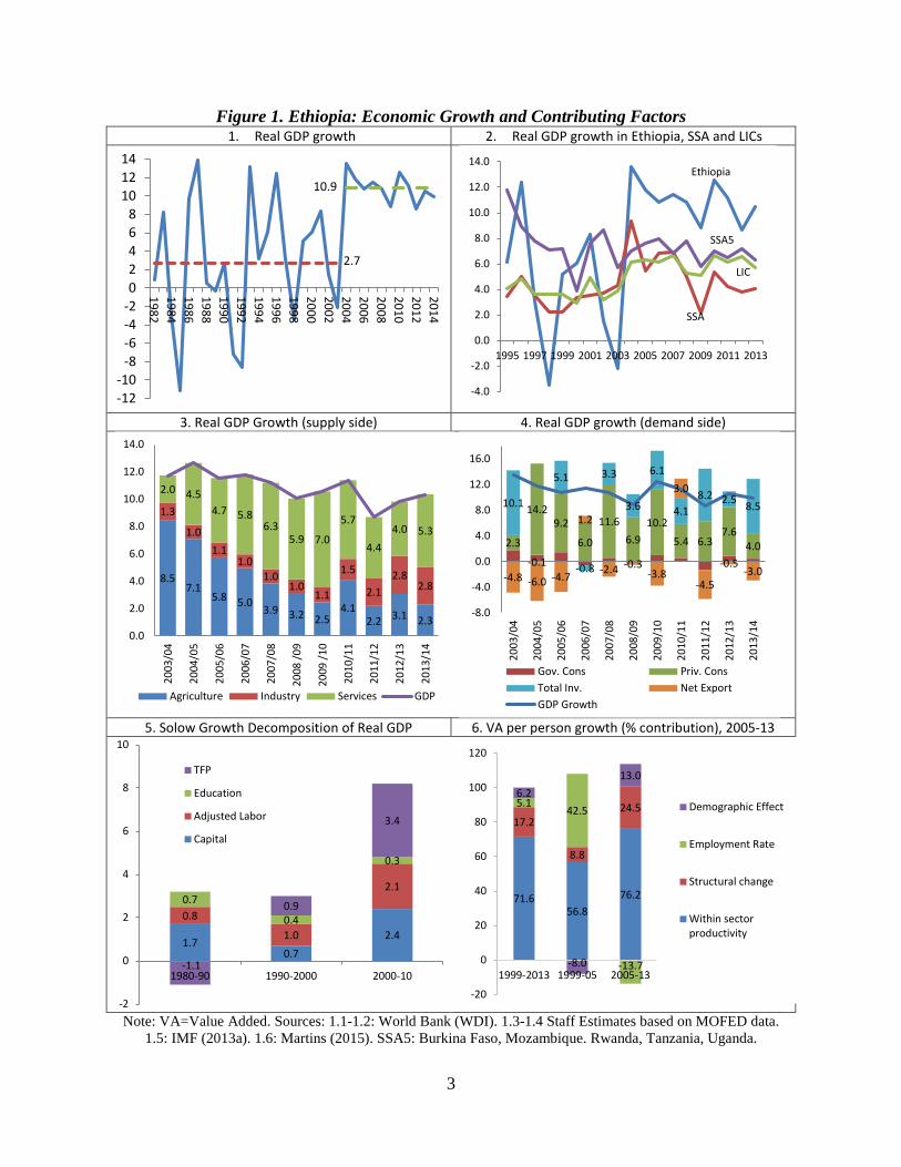
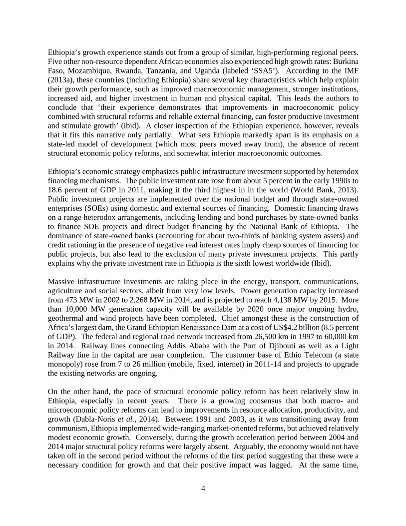
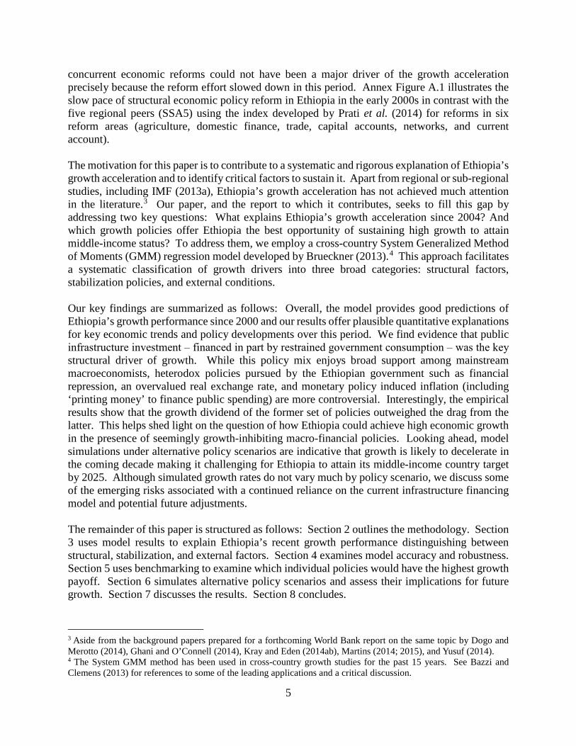
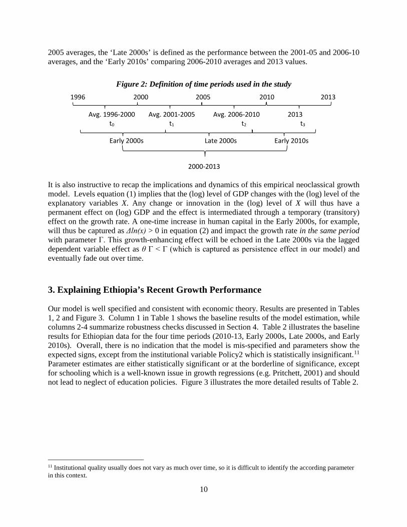
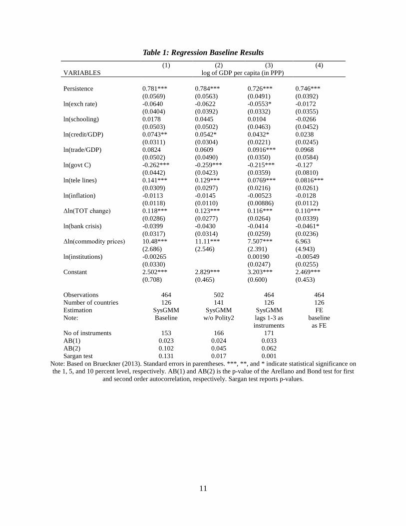
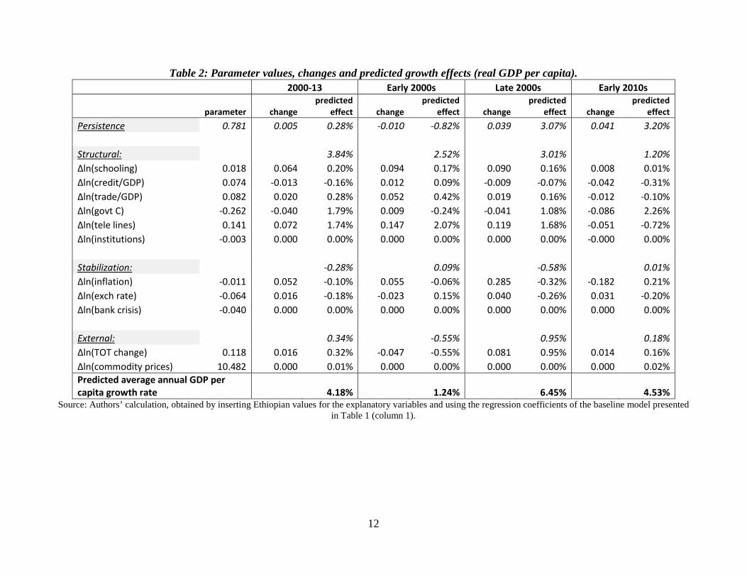
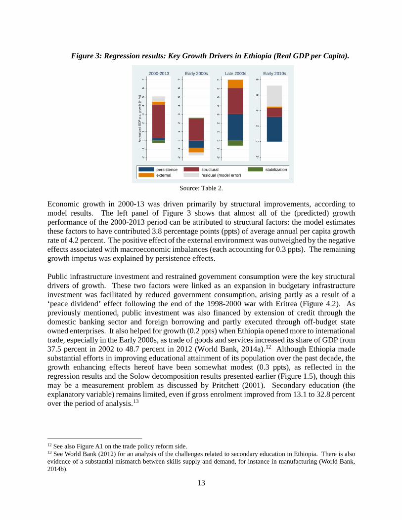
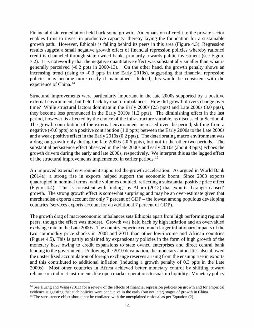
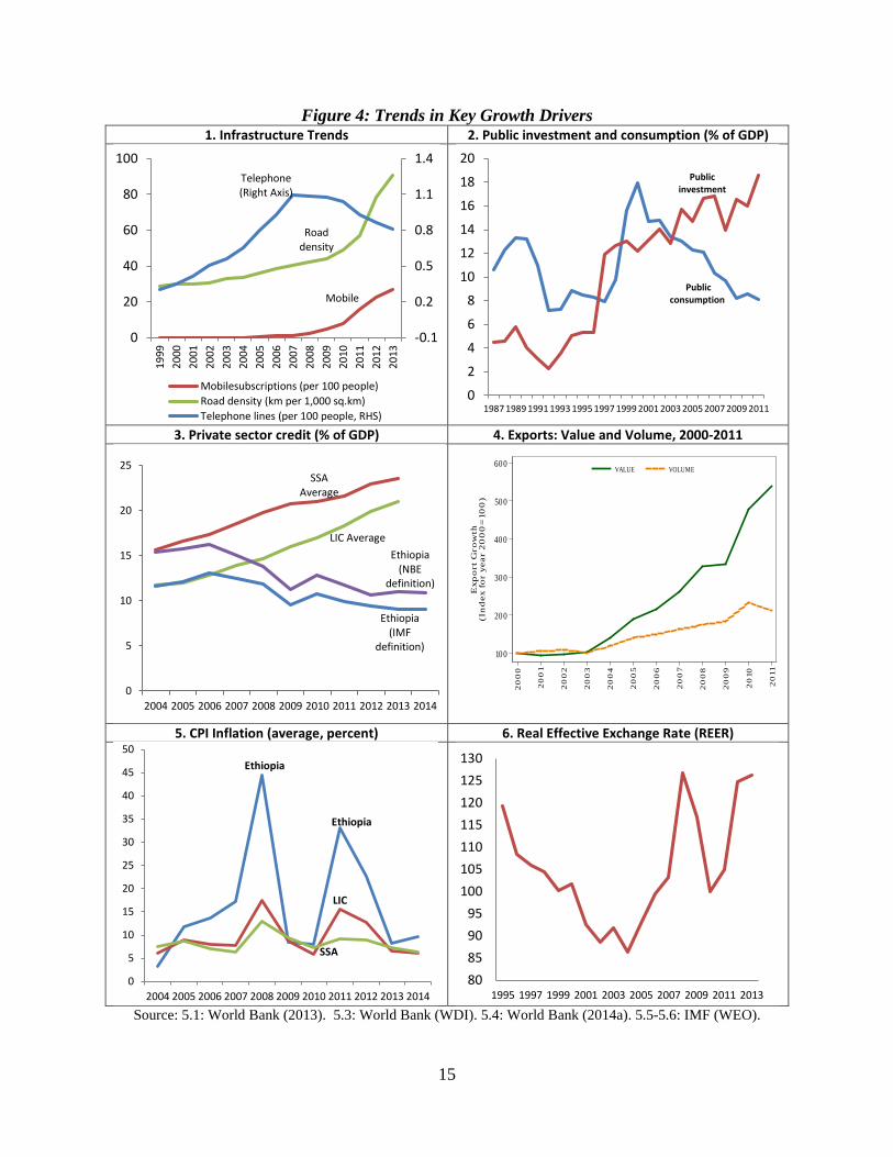
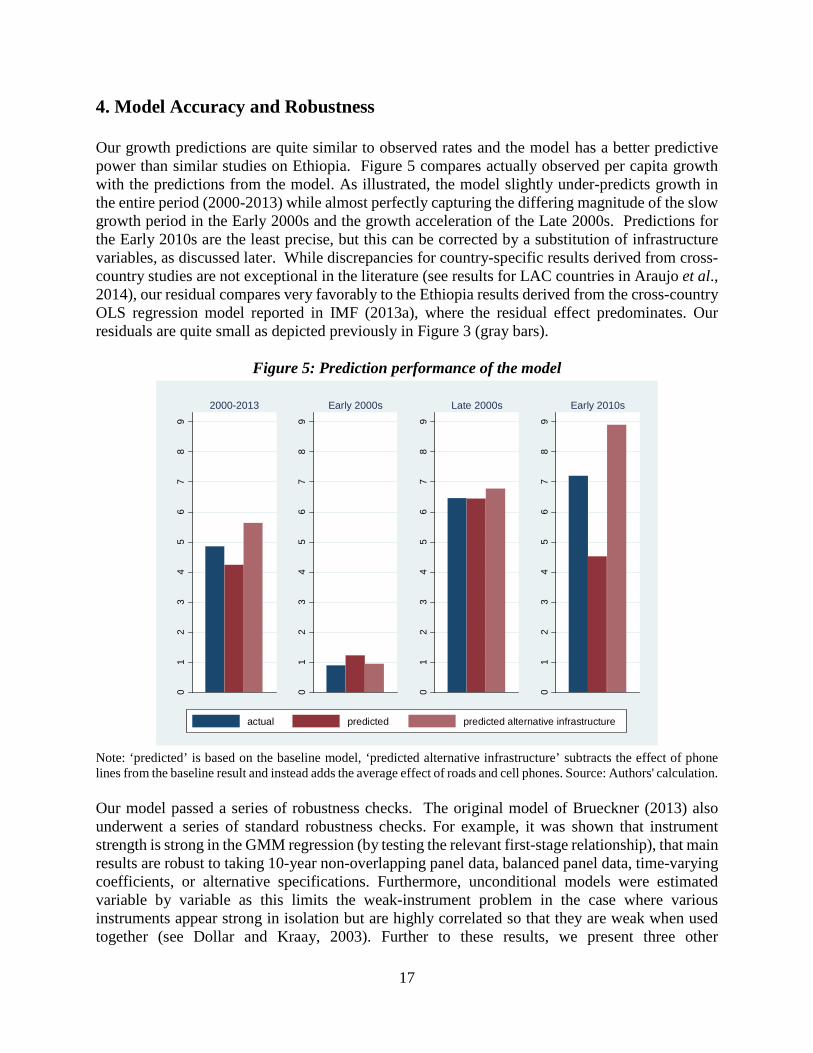
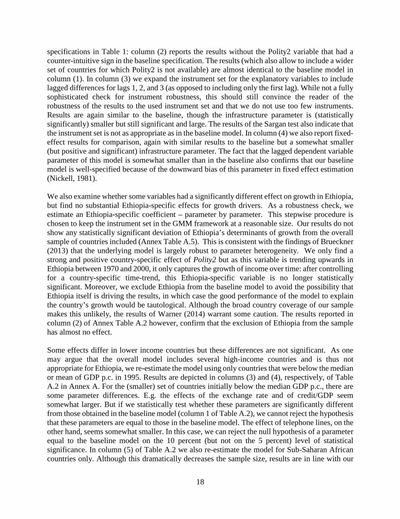
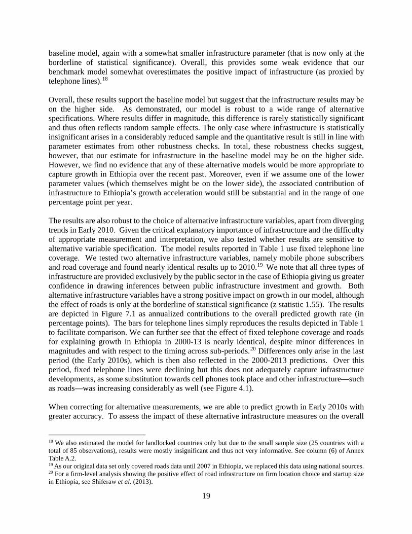
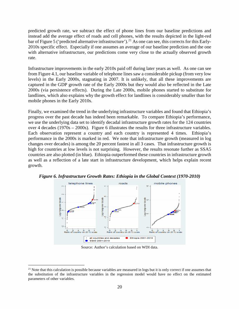
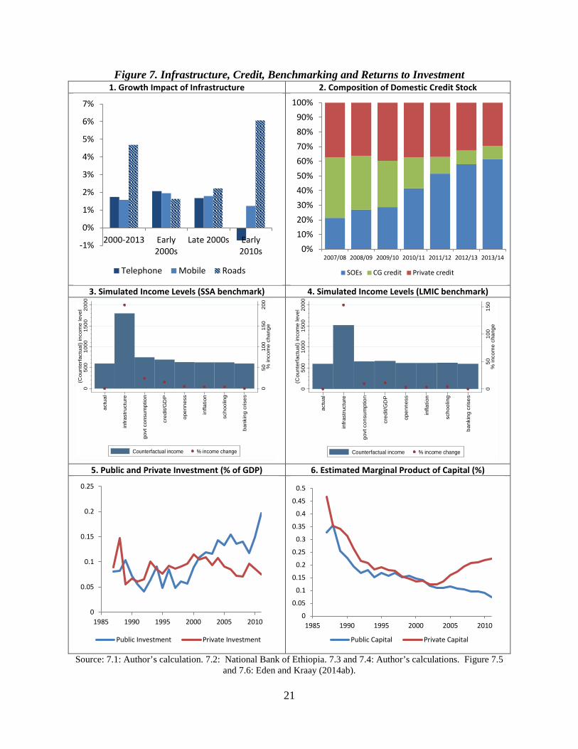
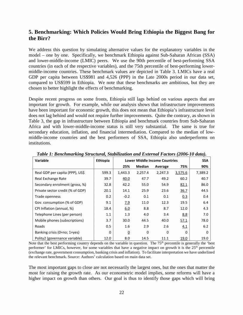
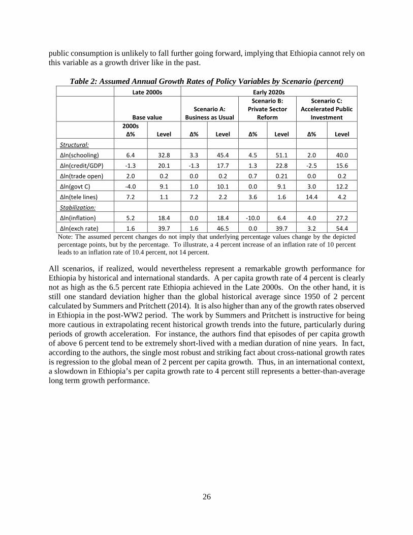
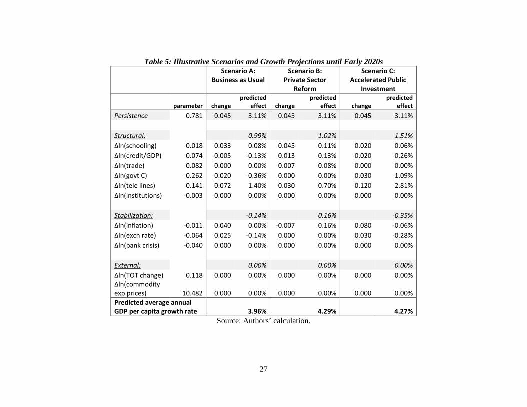
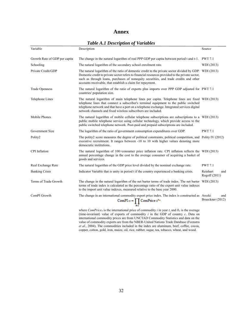
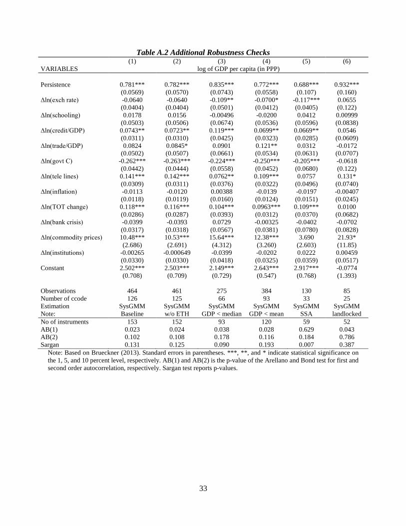
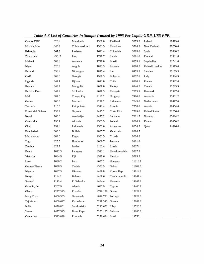
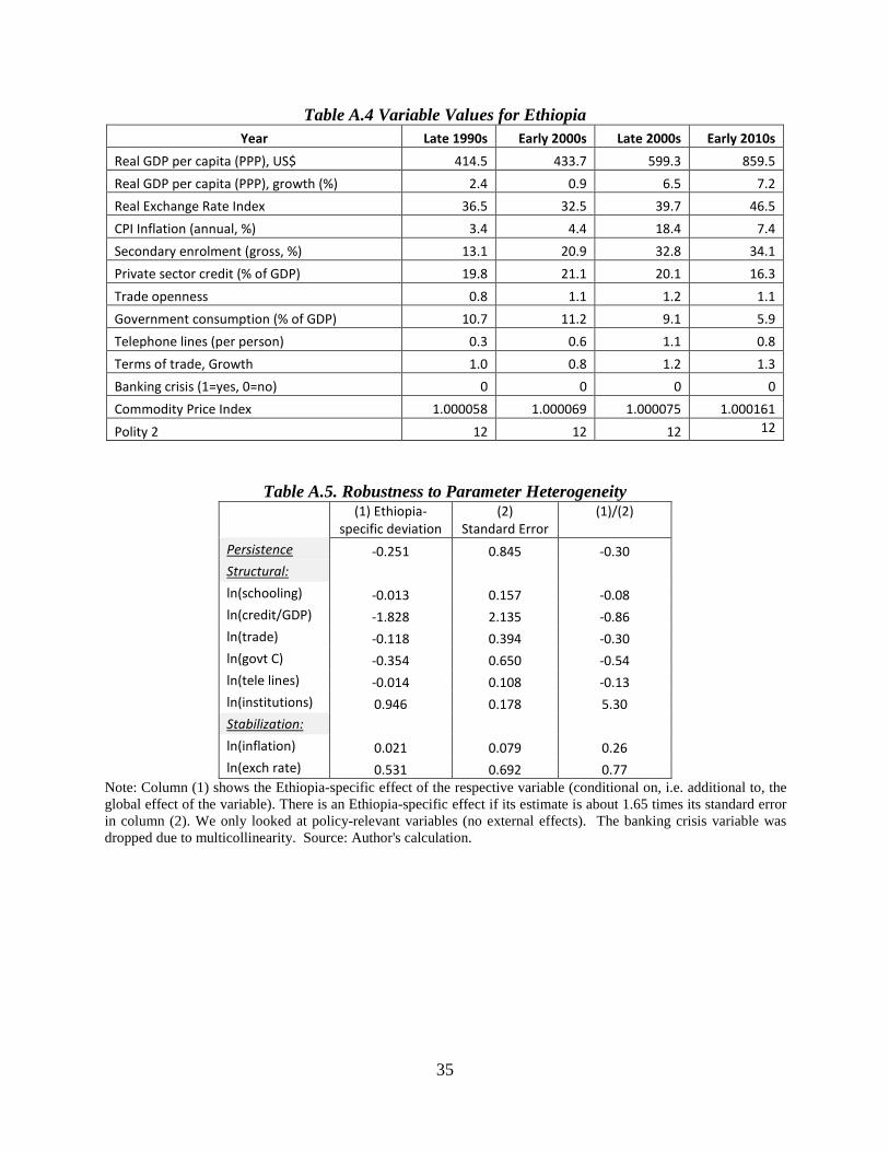
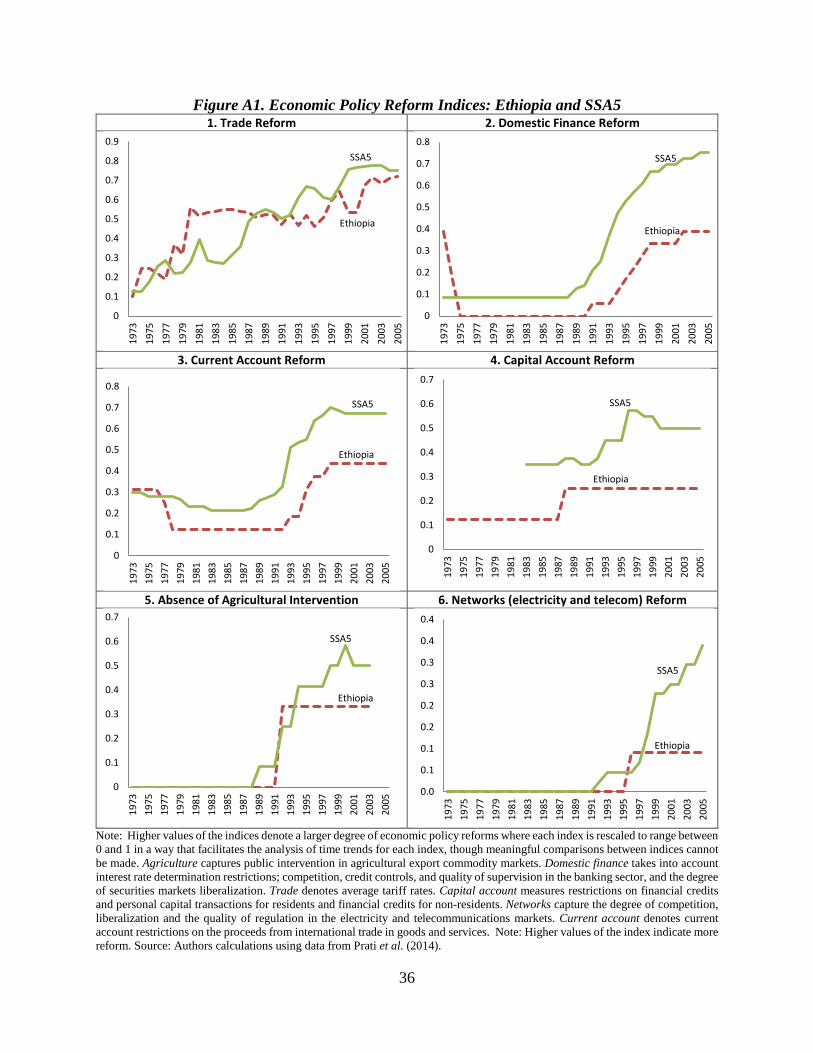


![ETHIOPIA’S MEDIUM TERM DEBT MANAGEMENT STRATEGY (2013 …siteresources.worldbank.org/INTDEBTDEPT/Resources/468980... · Ethiopia’s Medium Term Debt Strategy [2013-2017] Page 1](https://static.documents.pub/doc/80x56/5b1c3d1c7f8b9a1b688b5d65/ethiopias-medium-term-debt-management-strategy-2013-ethiopias-medium.jpg)


![Ethiopia’s nationhood reconsidered**analisesocial.ics.ul.pt/documentos/1317831305W4dWF... · to as Ethiopia’s national epic (Levine, 2000 [1974], the portrait of an early Hebraic](https://static.documents.pub/doc/80x56/5eb19706dc84c93ec16344a7/ethiopiaas-nationhood-reconsidered-to-as-ethiopiaas-national-epic-levine.jpg)


