EVALUATING THE ECONOMIC SIGNIFICANCE OF DOWNWARD NOMINALWAGE RIGIDITY
Michael W. Elsby
Working Paper 12611http://www.nber.org/papers/w12611
NATIONAL BUREAU OF ECONOMIC RESEARCH1050 Massachusetts Avenue
Cambridge, MA 02138October 2006
I am particularly grateful to my advisor, Alan Manning, for his perceptive comments and continuedpatience and encouragement. In addition I would like to thank Andrew Abel, Joseph Altonji, DavidAutor, Marianne Bertrand, Stephen Bond, Juan Dolado, Lorenz Goette, Maarten Goos, Steinar Holden,Francis Kramarz, Richard Layard, Stephen Machin, Jim Malcomson, Sendhil Mullainathan, StevePischke, Matthew Rabin, and Jennifer Smith for valuable comments. I would also like to thank seminarparticipants at the University of Michigan, Birkbeck, the Boston Fed, Chicago GSB, the CEPR ESSLE2004, European Winter Meetings of the Econometric Society 2004, Federal Reserve Board, Oslo,Oxford, Stockholm IIES, Warwick, and Zurich, for helpful suggestions. Any errors are my own. Theviews expressed herein are those of the author(s) and do not necessarily reflect the views of the NationalBureau of Economic Research.
Evaluating the Economic Significance of Downward Nominal Wage RigidityMichael W. ElsbyNBER Working Paper No. 12611October 2006JEL No. E24,E31,J30,J41
ABSTRACT
This paper formalizes and assesses empirically the implications of widely observed evidence for downwardnominal wage rigidity (DNWR). It shows how a model of DNWR informed by diverse evidence forworker resistance to nominal wage cuts is nevertheless consistent with weak macroeconomic effects.This occurs because firms have an incentive to compress wage increases as well as wage cuts whenDNWR binds. By neglecting potential compression of wage increases, the previous literature mayhave overstated the costs of DNWR to firms. Using a broad range of micro--data from the US andGreat Britain I find that firms do indeed compress wage increases as well as wage cuts at times whenDNWR binds. Accounting for this reduces the estimated increase in aggregate wage growth due toDNWR to be much closer to zero, consistent with the predictions of the model. These results suggestthat DNWR may not provide a strong argument against the targeting of low inflation rates, as practicedby many monetary authorities. Importantly, though, this result is nevertheless consistent with evidencethat suggests workers are averse to nominal wage cuts.
Michael W. ElsbyUniversity of MichiganDepartment of Economics238 Lorch Hall611 Tappan StreetAnn Arbor, MI 48109-1220and [email protected]
1 Introduction
A key stylized fact of modern economies is the apparent downward rigidity of nominal wages at
the individual level. A burgeoning literature has detailed striking features of the distribution of
nominal wage growth using micro-data. One of the most prominent features in these data is a large
mass point at zero nominal wage change. In addition, there are very few nominal wage cuts relative
to the number of nominal wage increases. Taken together, these facts strongly suggest the presence
of downward nominal wage rigidity (henceforth DNWR). Such evidence has been found in many
datasets covering many economies (for surveys see Kramarz, 2001, and Dickens et al., 2006).
Remarkably, this evidence dovetails with at least two other independent literatures in economics.
The �rst literature conducts surveys of wage-setters and negotiators to analyze their wage setting
behavior (see Bewley, 1999, and the survey in Howitt, 2002). Many of the respondents say that
they are reluctant to cut the nominal wages of workers. In particular, by interviewing over 300
managers, pay professionals, labor leaders etc., Bewley �nds that the most common explanation
provided for this reluctance is the belief that nominal wage cuts damage worker morale, and that
morale is a key determinant of worker productivity.
The second related literature presents additional evidence that people are averse to nominal
losses in an array of di¤erent economic settings (Sha�r, Diamond & Tversky, 1997). A typical
�nding is that respondents feel that it is much more acceptable to receive a 5% nominal wage
increase when in�ation is 12%, than a 7% wage cut when there is no in�ation (Kahneman, Knetsch
& Thaler, 1986). Similar sentiments are corroborated by Genesove & Mayer (2001) who �nd
evidence from real-estate data that condominium owners were reluctant to sell at a nominal price
below that they originally paid, even though they were typically moving locally, and hence were
buying in the same market.
Such evidence is all the more remarkable as economists have long speculated that DNWR is
fundamental to the workings of the macro-economy (Keynes, 1936; Tobin, 1972). In particular,
it has been claimed that DNWR implies the existence of a greater Phillips curve trade-o¤ at low
rates of in�ation (Akerlof, Dickens & Perry, 1996). The intuition underlying these claims is quite
2
compelling. Low in�ation implies that reductions in real labor costs can only be e¤ected through
nominal wage cuts. If �rms are prevented from cutting nominal wages, then their only recourse
is to layo¤ workers, leading to increased unemployment. Thus, when in�ation is low, increased
in�ation can relax the constraint of DNWR on wage-setting for a signi�cant fraction of �rms, and
thereby reduce unemployment. This result has been of particular interest in recent years due to
the adoption of in�ation targeting by many monetary authorities as it implies that implementing
a low in�ation target could result in a persistent increase in unemployment.
In contrast to the micro-level evidence, empirical support for the macroeconomic e¤ects of
DNWR has been relatively scant. A typical reference is the analysis of Card & Hyslop (1997) for
the US. Their micro-level analysis �nds strong evidence that nominal wage cuts are restricted when
in�ation is low, and they conclude that the existence of DNWR leads to an increase in average
real wage growth of up to 1% per annum. Card & Hyslop then assess whether the predictions
of this micro-level evidence are corroborated by aggregate data. In contrast to their micro-level
results, Card & Hyslop�s state-level results are much weaker. While they �nd some evidence for
the existence of a Phillips curve trade-o¤, they obtain estimates that are too imprecise to conclude
that this trade-o¤ is stronger in periods of low in�ation.1 This presents a puzzle: if the micro-level
evidence for DNWR is so robust, why is the macro-level evidence so unpersuasive?
One potential explanation might be that wages do not play an allocative role in the labor mar-
ket (Barro, 1977). In theory, wages could remain rigid for long periods of time without violating
e¢ ciency because rents exist to the continuation of a worker-�rm match. When it becomes prof-
itable for a �rm to replace an incumbent worker at the current wage, the wage will be negotiated
downward to the extent that the match remains e¢ cient. Thus wage rigidity is consistent with
e¢ ciency.
In this paper I show how a model of DNWR in which the wage is allocative is nevertheless
consistent with relatively weak unemployment e¤ects of low in�ation. Based on the evidence cited
above, the model assumes that wage rigidity arises due to an aversion to nominal wage cuts on the1Weak macroeconomic e¤ects have also been found by Lebow, Saks & Wilson (1999) for the US, and by Nickell &
Quintini (2003) and Smith (2004) for the UK. Indeed, Lebow, Saks & Wilson coined the term "micro-macro puzzle"for the observed tension between micro- and macro-level estimates.
3
part of the workers.2 The key insight in the analysis is that nominal wage increases in this setting
are partially irreversible. Consider a �rm that raises the wage today, but reverses its decision by
cutting the wage by an equal amount tomorrow. When workers resist wage cuts, the net e¤ect on
productivity will be negative: today�s wage increase will raise productivity, but tomorrow�s wage
cut will reduce productivity by a greater amount. Thus, reversals of wage increases are costly to
�rms. In this sense we can think of there being an asymmetric adjustment cost to changing nominal
wages.3
This insight equips us with a fundamental prediction: �rms will compress wage increases as well
as wage cuts in the presence of DNWR. This occurs through two channels. First, forward-looking
�rms temper wage increases as a precaution against future costly wage cuts. Raising the wage
today increases the likelihood of having to cut the wage, at a cost, in the future. Second, even in
the absence of forward-looking behavior, DNWR raises the level of lagged wages in the economy,
so �rms do not have to raise wages as often or as much to obtain their desired wage level. These
properties of the model imply the perhaps surprising prediction that worker resistance to wage cuts
should have no e¤ect on aggregate wage growth.
These results have important implications for the previous empirical literature on DNWR. This
literature has assumed (implicitly or otherwise) that the existence of DNWR has no e¤ect on the
upper tail of the wage change distribution. In particular, this is a key identifying assumption in
Card & Hyslop (1997), and leads them to use the observed upper tail of the distribution of wage
changes to infer the properties of the lower tail in the absence of DNWR. The above prediction
that wage increases will be compressed indicates that this assumption may be misguided.4 By2Given the empirical evidence for worker resistance to wage cuts, it is surprising that there has not yet been an
explicit model of such wage rigidity in the literature. The need for an explicit model of wage-setting in the presenceof worker resistance to wage cuts has been noted in the literature: Sha�r, Diamond & Tversky (1997), p.371 write�Plausibly, the relationship [between wages and e¤ort] is not continuous: there is a discontinuity coming from nominalwage cuts.... A central issue is how to model such a discontinuity.�This sentiment is echoed more recently by Altonji& Devereux (2000), p.423 note 7 who write �[I]t is surprising to us that there is no rigorous treatment in the literatureof how forward looking �rms should set wages when it is costly to cut nominal wages.�
3Models of adjustment costs have been widely studied in the investment and labor demand literatures, typicallyin the form of continuous time Brownian models (Bentolila & Bertola, 1990, and Abel & Eberly, 1996, are closest inspirit to the model analyzed here). In contrast, we formulate and solve our model of partial irreversibility in discretetime. This is helpful for two reasons. First, since data are reported in discrete intervals, this method allows us to aligntheoretical and empirical concepts more naturally. Moreover, many wage contracts are renegotiated on an annualbasis, which is more consistent with a discrete-time setup.
4This is not to say that Card & Hyslop (1997) is any more subject to this criticism than other previous empirical
4
neglecting the compression of wage increases, previous empirical research may have overstated the
increase in aggregate wage growth due to DNWR, and thereby the costs of DNWR to �rms.
I seek evidence for these predictions using micro-data for the US and Great Britain. I �nd
signi�cant evidence that the upper tail of the wage change distribution exhibits a compression of
wage increases related to DNWR. In particular, I �nd that this limits the estimated increase in
aggregate real wage growth due to DNWR from around 1�1.5% to no more than 0.3%. This is
because �rms can �save�at least 75% of the increase in wage growth due to restricted wage cuts
by reducing nominal wage increases.
As an additional test of the implications of worker resistance to wage cuts, I show that the model
also implies that increased rates of turnover should mitigate the necessity for �rms to restrict wage
increases. This occurs because higher turnover reduces the probability that a given worker will stay
in the �rm an additional period, and thus renders the �rm more myopic when it sets wages. Thus
�rms do not need to compress wage increases as a precaution against future costly wage cuts to
the same extent. I �nd evidence for this hypothesis using data from Great Britain. This reinforces
the claim that a model of DNWR based on worker resistance to nominal wage cuts is a useful way
of understanding the empirical properties of wage setting.
Based on this evidence, I conclude that there is no reason to expect the macro e¤ects of DNWR
to be as large as previously envisaged, and therefore that it does not provide a strong argument
against the adoption of a low in�ation target. Importantly, however, this result is nevertheless
consistent with the diverse body of evidence that suggests workers resist nominal wages cuts.
The rest of the paper is organized as follows. Section 2 presents an explicit behavioral model of
wage-setting in the presence of worker resistance to nominal wage cuts; section 3 �eshes out some
of the predictions of these models that can be taken to the data; section 4 presents the empirical
methodology and the results obtained; section 5 concludes. Where possible, I omit technical details
from the main text, and relegate them to the appendices5.
work on DNWR. Rather, it is the clarity of the identifying assumptions in that paper that allows a particularly cleanpoint of contrast with the implications of the model and results of this paper.
5 In addition, we omit some of the more straightforward proofs to save space �these are available from the authoron request.
5
2 A Model of DNWR based on Worker Resistance to Wage Cuts
In this section I present an explicit model of downward nominal wage rigidity based on the obser-
vations detailed in the empirical literatures mentioned above. In particular, I study the optimal
nominal wage policies of worker-�rm pairs for whom the productivity of the worker (denoted e)
depends upon the wage as follows:
e = ln�!b
�+ c ln
�W
W�1
�1� (1)
where W is the nominal wage, W�1 the lagged nominal wage, 1� an indicator for a nominal wage
cut, ! � W=P the real wage, and b a measure of real unemployment bene�ts (which I assume to
be constant over time). The parameter c > 0 varies the productivity cost to the �rm of a nominal
wage cut.
The motivation for the qualitative features of this e¤ort function is as follows6. I assume that
worker e¤ort depends positively on the di¤erence between the level of the real wage, !, and real
unemployment bene�ts, b. This captures the idea that, the higher the worker�s real standard of
living from being in work relative to unemployment, the harder that worker will work. In addition,
I model the productivity loss due to nominal wage cuts by assuming that e¤ort is falling in the
geometric nominal wage cut. The reasoning for this is that the most obvious alternative �that
it is the absolute value of the cut in the nominal wage that reduces e¤ort �is implausible in the
following sense. It implies that a wage cut of a cent will cause the same loss in e¤ort whether last
period�s nominal wage is $1 or $1,000,000. This is clearly extreme, so I employ the more sensible
concept that it is the percentage cut in the nominal wage that a¤ects e¤ort7.
The qualitative features of this e¤ort function are illustrated in Figure 1. Clearly, there is a
6The precise parametric form of (1) is chosen primarily for analytical convenience. None of the qualitative resultsemphasized in what follows depends on the speci�c parametric form of (1) �the key is that e¤ort is increasing in thewage and kinked around the lagged nominal wage.
7One may be interested in a speci�cation with a �xed e¤ort cost due to wage cuts, or a more general convexity ofe¤ort in wage cuts informed by the literature on loss aversion (Kahneman & Tversky, 1979). Both such speci�cationswould lead employers to cut the wage dramatically if they cut the wage at all. This di¤ers from the model analyzedhere in that we would expect to see a �hole� in the density of wage changes to the left of zero. Whilst previousstudies have not found strong support for this (Card & Hyslop, 1997), further work may be worthwhile to assess thismore formally.
6
kink at W =W�1 re�ecting the existence of DNWR. In particular, the marginal productivity loss
of a nominal wage cut exceeds the marginal productivity gain of a nominal wage increase:
@e=@W jW"W�1
@e=@W jW#W�1
= 1 + c > 1 (2)
This characteristic is what makes nominal wage increases (partially) irreversible �a nominal wage
increase can only be reversed at an additional marginal cost of c. Clearly, this is the key driving
force in the model that I seek to analyze, and the parameter c is what drives this feature of the
model.
The e¤ort function, (1), can be interpreted as a very simple way of capturing the basic essence
of the motivations for DNWR mentioned in the literature. It is essentially a parametric form
of e¤ort functions in the spirit of the fair-wage e¤ort hypothesis expounded by Solow (1979) and
Akerlof & Yellen (1988), with an additional term re�ecting the impact of nominal wage cuts on
e¤ort �as envisaged in the evidence cited in the introduction. Bewley (1999) also advocates such
a characterization8:
�The only one of the many theories of wage rigidity that seems reasonable is the
morale theory of Solow...�Bewley (1999), p.423.
�The [Solow] theory...errs to the extent that it attaches importance to wage levels
rather than to the negative impact of wage cuts.�Bewley (1999), p.415.
In addition, an e¤ort function with these properties can be derived from a compensating di¤erentials
model where worker utility exhibits nominal loss aversion. The basic intuition for this is that, if
workers dislike nominal losses and the �rm wishes to cut the nominal wage, then the �rm must
compensate the worker in the form of lower on-the-job e¤ort in order to prevent the worker from
quitting. Thus, in this sense, (1) can be considered a reduced form of a model in which workers
dislike nominal loss. The goal of this paper is not to highlight the nuances of emphasis �which do
8However, such is the intricacy of Bewley�s study, he would probably consider (1) a simpli�cation, not least for itsneglect of emphasis on morale as distinct from productivity, and of the internal wage structure of �rms as a sourceof wage rigidity. We argue that it is a useful simpli�cation as it provides key qualitative insights into the implieddynamics of wage-setting under more nuanced theories of morale.
7
indeed exist �between these behavioral foundations, but rather to show that they share a common,
theoretically important, qualitative implication as to the nature of a �rm�s wage-setting choice.
This is intended as a start towards richer models of these phenomena, and to this end aims to unify
rather than to di¤erentiate.
The most comparable previous attempt at explicitly modelling the behavioral foundation to
DNWR is that of Akerlof, Dickens & Perry (1996). However, Akerlof et al. present a model in
which �rms have no operational discretion over wage-setting �wages are given by a wage-setting
relationship which �rms take as exogenous, and which dictates that nominal wages can never fall.
Thus, the implicit assumption in their model is that �rms do not cut wages because, if they did, all
of their workers would quit. The model presented in this paper di¤ers critically in that �rms have a
non-trivial wage-setting decision: �rms can cut nominal wages if they wish, but it will have a strong
adverse e¤ect on productivity at the margin. I argue that this is a more desirable setup. In the
�rst instance, it accords better with the evidence that �rms restrict wage cuts due to concerns over
morale within the �rm, rather than because the external labor market dictates it (Bewley, 1999).
Secondly, I will show that a model with wage discretion captures an important characteristic of the
available data: that wage increases are also compressed when DNWR binds.
The Wage Setting Problem
I consider a discrete-time, in�nite-horizon model in which price-taking worker-�rm pairs choose
the nominal wage Wt at each date t to maximize the expected discounted value of pro�ts. For
simplicity, I assume that each worker-�rm�s production function is given by a � e, where a is a real
technology shock that is idiosyncratic to the worker-�rm match, is observed contemporaneously,
and acts as the source of uncertainty in the model. Thus, de�ning � 2 [0; 1) as the discount factor
of the �rm, the typical �rm�s decision problem is given by:
maxfWtg
Et
" 1Xs=t
�s�t fases � !sg#
(3)
where es = ln�!sb
�+ c ln
�Ws
Ws�1
�1�s
8
It turns out in what follows that it is convenient to re-express the �rm�s pro�t stream in constant
date t prices. To this end, I multiply through by Pt, which I de�ne as the competitive price level at
date t, and assume that it evolves according to Pt = (1 + �)Pt�1, where � is the rate of in�ation.
Finally, de�ning the nominal counterparts, At � Ptat and Bt � Ptb and substituting for et, I obtain
the following optimization problem for the �rm:
maxfWtg
Et
" 1Xs=t
��
1 + �
�s�t�As
�ln
�Ws
Bs
�+ c ln
�Ws
Ws�1
�1�s
��Ws
�#(4)
I assume that the nominal shock has support [0;1) and that its evolution can be described by the
cumulative density function F (A0jA). Thus, rewriting the problem in recursive form9 I have10:
v (W�1; A) = maxW
�A
�ln
�W
B
�+ c ln
�W
W�1
�1���W +
�
1 + �
Zv�W;A0
�dF�A0jA
��(5)
(5) is the basic problem that I will attempt to solve in what follows11.
2.1 Some Intuition for the Model
To anticipate the model�s results, in this section I present the economic intuition for each of the
predictions of the model. First, the model predicts that there will be a spike at zero in the
distribution of nominal wage changes across �rms. This occurs because of the kink in the objective
function at W =W�1. In particular, this implies that for each �rm there will be a range of values
(�region of inaction�) for the nominal shock, A, for which it is optimal not to change the nominal
wage. Since A is distributed across �rms, there will exist a positive fraction of �rms each period
whose realization of A lies in their region of inaction that will in turn not change their nominal
wage.
9We adopt the convention of denoting lagged values by a subscript, �1, and forward values by a prime, 0.10 In addition, we make the assumptions that the measure dF (A0jA) satis�es the Feller property and is monotone,
so that the mapping (5) preserves continuity of the value function, and monotonicity of the value function in A. Asu¢ cient condition for this is that A is governed by the stochastic di¤erence equation, A0 = g (A; "0), where g is acontinuous function, "0 is an i.i.d. innovation (see Stokey & Lucas, 1989, pp.237, 261�262), and gA > 0. We maintainthese assumptions throughout the paper.11There is an issue that, for su¢ ciently low values of the wage, e¤ort is potentially negative. However, accounting
for such a non-negativity constraint signi�cantly complicates the solution to the model without much gain in relevance.We maintain the assumption that the level of bene�ts is su¢ ciently low relative to wages as to allow almost all �rmsto ignore this constraint.
9
Second, in the event that a �rm does decide to change the nominal wage, the wage change will
be actively compressed relative to the case where there is no DNWR. That nominal wage cuts are
attenuated is straightforward to explain �as wage cuts involve a discontinuous fall in productivity
at the margin, the �rm will be less willing to implement them. In particular, some small wage cuts
that would have been implemented in the absence of DNWR will instead be implemented as wage
freezes. Moreover, larger counterfactual wage cuts will be reduced in magnitude. It is slightly
less obvious why nominal wage increases are also attenuated in this way. The reason is that, in an
uncertain world, increasing the wage today increases the likelihood that the �rm will have to cut
the wage, at a cost, in the future.
A direct implication of this last prediction is that increases in the productivity cost of cutting
the nominal wage, c, will accentuate all these e¤ects. That is, a higher productivity cost due to
nominal wage cuts will widen the region of inaction, thereby increasing the mass point at zero in
the distribution of nominal wage changes, and will also render the active compression of nominal
wage changes more acute.
An additional, perhaps more fundamental e¤ect that obtains from the model even in the absence
of active compression is what I will refer to as �latent compression�of wage increases. This e¤ect
captures the idea that an inability on behalf of �rms to cut wages will tend to raise the wages
that �rms inherit from the past. As a result, when raising wages, �rms do not have to increase
wages by as much or as often in order to achieve their optimal wage. Thus, this process of latent
compression works in tandem with the active compression of wage increases outlined above12.
The �nal prediction to emphasize at this stage is the e¤ect of increased in�ation on nominal
wage increases. In particular, the active compression of nominal wage increases becomes less
pronounced as in�ation rises. As explained earlier, this is because the only reason �rms restrict
wage increases in the model is the prospect of costly nominal wage cuts in the future. Since higher
in�ation reduces the probability of this occurring, �rms no longer need to worry as much about
12 Identifying this additional e¤ect is an important bene�t of the in�nite horizon model studied here. In particular,one might imagine that active compression-type results could be obtained from a �simpler�two-period model. Latentcompression will be shown to be an outcome of steady state considerations, which cannot be treated in a two-periodcontext.
10
increasing the nominal wage.13
2.2 The Dynamic Model
The basic structure of the solution to the full dynamic model, (5), is as follows. I solve the problem
by �rst taking the �rst-order condition with respect to W , conditional on �W 6= 0:
�1 + c1�
� AW� 1 + �
1 + �D (W;A) = 0; if �W 6= 0 (6)
where D (W;A) �RvW (W;A
0) dF (A0jA) is the marginal e¤ect of the current wage choice on the
future pro�ts of the �rm. Clearly, a key step in solving for the �rm�s optimal wage policy involves
characterizing the properties of the function D (�). For the moment, however, note �rst that the
general structure of the optimal nominal wage policy is as follows:
Proposition 1 The optimal nominal wage policy in the dynamic model is of the form:
If A > u (W�1) � Au; �W > 0 until W = u�1(A)
If A < l (W�1) � Al; �W < 0 until W = l�1 (A)
If A 2 [Al; Au] ; �W = 0 or W =W�1
(7)
where the functions u (�) and l (�) satisfy:
u (W )
W� 1 + �
1 + �D (W;u (W )) � 0 (8)
(1 + c)l (W )
W� 1 + �
1 + �D (W; l (W )) � 0
The reasoning for this is very straightforward. Proposition 1 uses the conditional �rst-order
condition (6) to de�ne the functions u (�) and l (�), as in (8). These functions determine the optimal13One might think that a standard model of menu costs predicts a compression of wage increases in times of low
in�ation. Intuitively, as �rms increase prices less often to avoid successive payment of menu costs in high in�ationenvironments, when they do increase the price, they will increase it by a greater amount. However, if this werethe correct model, one would expect to see �holes� either side of zero in the density of nominal wage changes, andmoreover that these holes would widen as in�ation rises. Whilst previous empirical work has found some evidencefor menu cost e¤ects, these e¤ects have only a modest impact on wage changes around zero (Card & Hyslop, 1997),and certainly are not accentuated in times of high in�ation.
11
relationship between the nominal wage, W , and the nominal shock, A, in the event that wages are
adjusted up or down respectively. The rest of the result follows from the fact that, by virtue of the
continuity and concavity of the �rm�s objective, (5), the optimal value of W must be a continuous
function of A14.
However, to complete the characterization of the �rm�s optimal nominal wage policy, it is
necessary to establish the functions u (�), and l (�). In particular, it can be seen from (8) that,
in order to solve for these functions, one requires knowledge of the functions D (W;u (W )) and
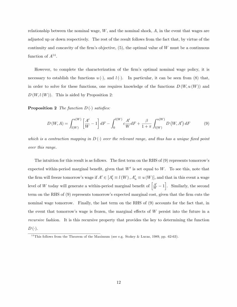
D (W; l (W )). This is aided by Proposition 2:
Proposition 2 The function D (�) satis�es:
D (W;A) =
Z u(W )
l(W )
�A0
W� 1�dF �
Z l(W )
0cA0
WdF +
�
1 + �
Z u(W )
l(W )D�W;A0
�dF (9)
which is a contraction mapping in D (�) over the relevant range, and thus has a unique �xed point
over this range.
The intuition for this result is as follows. The �rst term on the RHS of (9) represents tomorrow�s
expected within-period marginal bene�t, given that W 0 is set equal to W . To see this, note that
the �rm will freeze tomorrow�s wage if A0 2 [A0l � l (W ) ; A0u � u (W )], and that in this event a wage
level of W today will generate a within-period marginal bene�t ofhA0
W � 1i. Similarly, the second
term on the RHS of (9) represents tomorrow�s expected marginal cost, given that the �rm cuts the
nominal wage tomorrow. Finally, the last term on the RHS of (9) accounts for the fact that, in
the event that tomorrow�s wage is frozen, the marginal e¤ects of W persist into the future in a
recursive fashion. It is this recursive property that provides the key to determining the function
D (�).14This follows from the Theorem of the Maximum (see e.g. Stokey & Lucas, 1989, pp. 62-63).
12
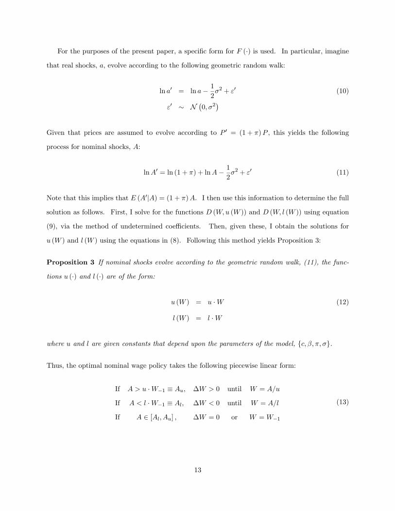
For the purposes of the present paper, a speci�c form for F (�) is used. In particular, imagine
that real shocks, a, evolve according to the following geometric random walk:
ln a0 = ln a� 12�2 + "0 (10)
"0 � N�0; �2
�Given that prices are assumed to evolve according to P 0 = (1 + �)P , this yields the following
process for nominal shocks, A:
lnA0 = ln (1 + �) + lnA� 12�2 + "0 (11)
Note that this implies that E (A0jA) = (1 + �)A. I then use this information to determine the full
solution as follows. First, I solve for the functions D (W;u (W )) and D (W; l (W )) using equation
(9), via the method of undetermined coe¢ cients. Then, given these, I obtain the solutions for
u (W ) and l (W ) using the equations in (8). Following this method yields Proposition 3:
Proposition 3 If nominal shocks evolve according to the geometric random walk, (11), the func-
tions u (�) and l (�) are of the form:
u (W ) = u �W (12)
l (W ) = l �W
where u and l are given constants that depend upon the parameters of the model, fc; �; �; �g.
Thus, the optimal nominal wage policy takes the following piecewise linear form:
If A > u �W�1 � Au; �W > 0 until W = A=u
If A < l �W�1 � Al; �W < 0 until W = A=l
If A 2 [Al; Au] ; �W = 0 or W =W�1
(13)
13
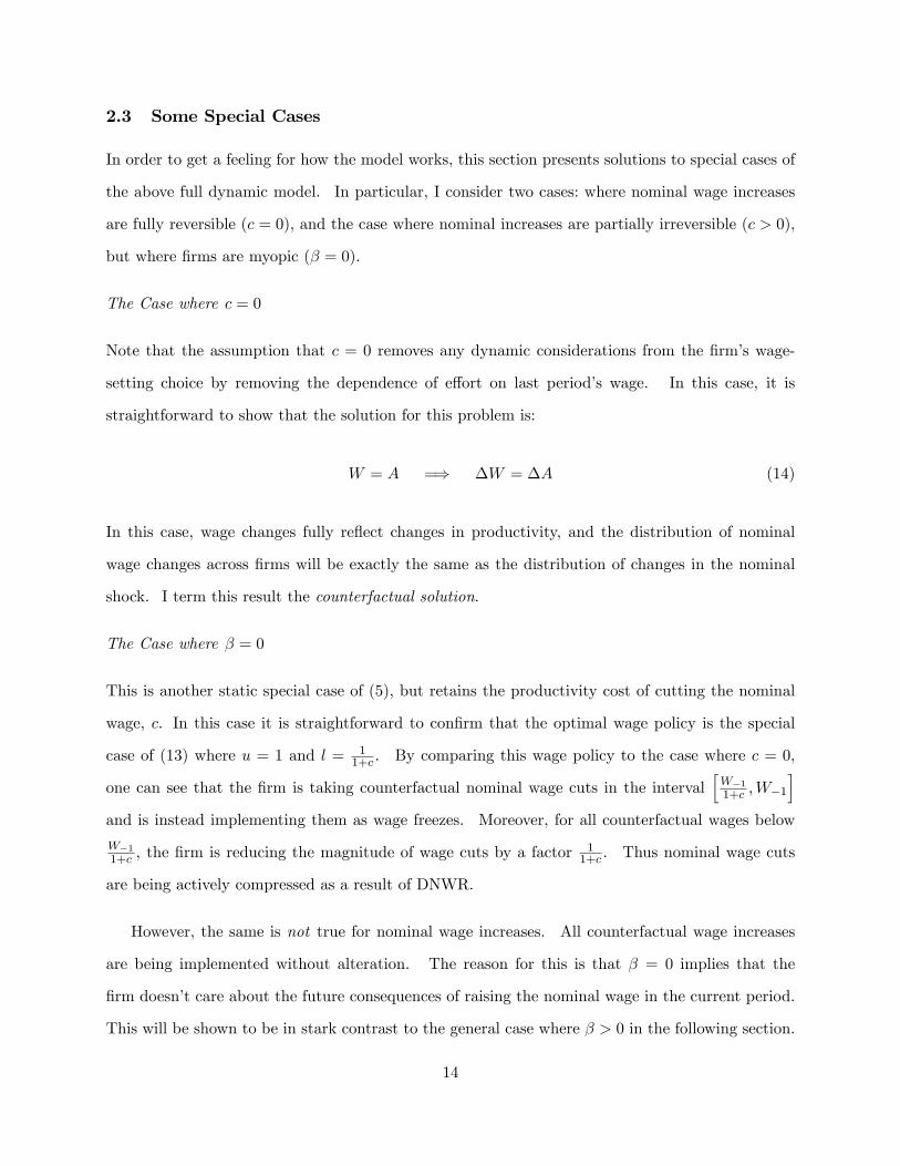
2.3 Some Special Cases
In order to get a feeling for how the model works, this section presents solutions to special cases of
the above full dynamic model. In particular, I consider two cases: where nominal wage increases
are fully reversible (c = 0), and the case where nominal increases are partially irreversible (c > 0),
but where �rms are myopic (� = 0).
The Case where c = 0
Note that the assumption that c = 0 removes any dynamic considerations from the �rm�s wage-
setting choice by removing the dependence of e¤ort on last period�s wage. In this case, it is
straightforward to show that the solution for this problem is:
W = A =) �W = �A (14)
In this case, wage changes fully re�ect changes in productivity, and the distribution of nominal
wage changes across �rms will be exactly the same as the distribution of changes in the nominal
shock. I term this result the counterfactual solution.
The Case where � = 0
This is another static special case of (5), but retains the productivity cost of cutting the nominal
wage, c. In this case it is straightforward to con�rm that the optimal wage policy is the special
case of (13) where u = 1 and l = 11+c . By comparing this wage policy to the case where c = 0,
one can see that the �rm is taking counterfactual nominal wage cuts in the intervalhW�11+c ;W�1
iand is instead implementing them as wage freezes. Moreover, for all counterfactual wages below
W�11+c , the �rm is reducing the magnitude of wage cuts by a factor 1
1+c . Thus nominal wage cuts
are being actively compressed as a result of DNWR.
However, the same is not true for nominal wage increases. All counterfactual wage increases
are being implemented without alteration. The reason for this is that � = 0 implies that the
�rm doesn�t care about the future consequences of raising the nominal wage in the current period.
This will be shown to be in stark contrast to the general case where � > 0 in the following section.
14
However, it should be noted at this point that even in this simple case the methods of previous
empirical studies will be potentially biased. Whilst this special case yields no active compression
of wage increases by �rms, there will still be some latent compression: since DNWR places upward
pressure on the level of wages in the past, the �rm does not have to raise wages as frequently to
achieve their target wage today.
3 Predictions
3.1 Active Compression
Returning to the more general solution in (13), it can be seen that active compression of wage
changes can be related to the parameters u and l. Numerical simulations of the model establish
that u > 1 > l and that 1=l > u.15 This is precisely in accordance with the intuition in section 2.1.
Since u > l there exists a region of inaction for the nominal shock variable in which it is optimal
not to change the nominal wage. Moreover, because l < 1 there will be an active compression
of nominal wage cuts. This follows directly from the discontinuous fall in e¤ort following a wage
cut at the margin. In addition, u > 1 means that nominal wage increases will also be actively
compressed relative to the counterfactual solution. Recall that the intuition for this is that raising
the nominal wage today raises the likelihood that the �rm will wish to cut the wage, at a cost, in
the future. Finally, the fact that 1=l > u implies that the active compression of wage increases will
not be as strong as that for wage cuts. The reason for this is that the potential costs associated
with wage increases are discounted in two ways. First, some discounting derives from the fact that
raising the wage may only increase the costs of wage cuts in the future. But, in addition to this,
the probability that these additional future costs will be realized is less than one, leading to further
discounting.
Recall that a key concern is with the characteristics of the nominal wage change distribution.
Using (13) it is straightforward to establish the following result on the form of the log nominal
wage change distribution, conditional on the lagged wage:
15Unfortunately, due to the analytical complexity of the solution, a formal proof of this result has proved elusive.
15
Proposition 4 The log nominal wage change density, conditional on the lagged wage, implied by
the model of section 2 is given by:
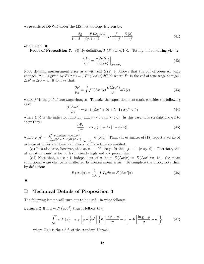
f (� lnW jW�1) =
8>>>><>>>>:~f (� lnW + lnujW�1) if � lnW > 0
~F (lnujW�1)� ~F (ln ljW�1) if � lnW = 0
~f (� lnW + ln ljW�1) if � lnW < 0
(15)
where ~F (�jW�1) and ~f (�jW�1) are the c.d.f. and p.d.f. of the counterfactual (no DNWR) condi-
tional log nominal wage change distribution.
Figure 2 illustrates this result. In particular, it shows that the distribution of log wage cuts is
exactly the same as the counterfactual distribution below ln l < 0, just shifted horizontally by an
amount � ln l > 0. A symmetric result obtains for wage increases. The residual density is �piled
up�to a mass point at zero wage change. Thus, the e¤ect of worker resistance to wage cuts is to
yield a conditional log wage change distribution with dual censoring from above and below relative
to the counterfactual16.
The key prediction that will be tested in the following empirical work is the e¤ect of the rate of
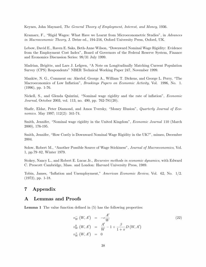
in�ation, �, on the compression of nominal wage increases. To this end, �gure 3 presents results
for the e¤ect of changes in the rate of in�ation on the parameter u. It is clear is that the �rm
will reduce any active compression of wage increases as in�ation rises since u falls as � rises. The
intuition for this is that active compression of wage increases occurs only insofar as wage increases
raise the likelihood of future costly nominal wage cuts. To see this, note that the special case
in which the �rm does not care about the future (� = 0) yielded no active compression of wage
increases (u = 1). Thus, since higher in�ation reduces the likelihood of future costly nominal cuts,
the �rm no longer needs to worry about raising the nominal wage today. A key related result is
that as in�ation becomes large, u! 1. That is, high in�ation implies that wage increases cease to
be actively compressed relative to a counterfactual world without DNWR. Thus, if the model of
section 2 is correct, one would expect to observe the upper tail of f (� lnW jW�1) becoming more
16This censoring result has interesting parallels in the previous empirical literature. Altonji & Devereux (2000)estimate an econometric model similar to (15) except that they do not account for the possibility of compression ofwage increases.
16
dispersed as in�ation rises. This is illustrated in Figure 4. However, this is not the end of the
story: the next section shows that there are additional reasons for there to be a compression of
wage increases, even in the absence of these e¤ects.
3.2 Latent Compression
All of the above discussion on active compression has been in terms of the nominal wage change
distribution conditional on the lagged nominal wage. The reason for this is that the lagged wage is
taken as given (is part of the state) at the time of setting the current wage, and so all theories will
yield direct implications on the conditional distribution, f (� lnW jW�1). However, most of the
previous empirical literature has concentrated on the properties of the unconditional distribution,
f (� lnW ), typically by estimating some measure of the increase in average wage growth due to
DNWR, E (� lnW jDNWR)�E (� lnW jno DNWR), to try to gain an impression of the e¤ect of
DNWR on the �rms�real labor costs. The following proposition demonstrates that this emphasis
in the previous literature may well be misleading:
Proposition 5 DNWR has no e¤ect on average wage growth in the long run for �nite G � u=l.
This result can be interpreted in a number of ways. First, and closest to the form of the proof,
note that the optimal wage policy (13) implies that the di¤erence in the levels of the log wage with
and without DNWR must be bounded (between � lnu < 0 and � ln l > 0). Thus, it follows that
the rates of growth of actual and counterfactual log wages cannot be di¤erent in the long run, as it
would necessarily imply a violation of these bounds.17
An alternative interpretation for this result is that it is simply a requirement for the existence of
a steady state in which average growth rates are equal. Since productivity shocks grow on average
at a constant rate, so must wages grow at that same rate in the long run. Thus, even the model
with DNWR must comply with this simple steady state condition in the long run.
How might this result come about? First, the results above indicate that �rms may actively
compress wage increases as a precaution against future costly wage cuts, thereby limiting the wage
17A similar result has been established independently in the investment literature by Bloom (2000).
17
growth increasing e¤ects of DNWR. However, this cannot be the whole story �we saw above that
the active compression of wage increases will be less than that of wage cuts. In addition, consider
the case where � = 0. Recall that this is the case in which there is no active compression of wage
increases as �rms are myopic. Figure 5 shows a simulation of the unconditional wage change
distribution implied by the behavioral model in this case. It can be seen from Figure 5 that,
contrary to the assumption of previous studies, the upper tail of f (� lnW ) displays a compression
in the presence of DNWR. Thus, the upper tail of the wage change distribution is still compressed,
even if �rms do not actively compress wage increases.
This provides an additional insight into the process by which this steady state requirement
might be achieved in practice. If wage increases are not actively compressed, this means that when
�rms increase the wage, they increase it to the counterfactual level, A. However, recall that the
existence of DNWR will tend to raise the general level of lagged wages in the economy, as �rms
will have been constrained in cutting wages in the past. Thus, when �rms increase the wage, they
do not have to increase it by as much or as often to reach the counterfactual wage level. Thus the
upper tail of f (� lnW ) will indeed still be a¤ected by the existence of DNWR �in particular, it
will be less dispersed, as seen in Figure 5. I term this additional e¤ect �latent compression�.
3.3 The Costs of DNWR to Firms
Proposition 5 has important implications with respect to the previous empirical literature. First,
by not taking into account the compression of wage increases, previous empirical studies could have
overstated the increase in wage growth due to DNWR. To see this, consider Figure 6. This shows
three simulated wage change distributions derived from the model of section 2. The bold line
shows the wage change distribution with DNWR (c > 0), whereas the thick dashed line illustrates
the true counterfactual wage change density (c = 0). In addition, I include a �median symmetric�
(hereafter MS) counterfactual density that is derived by imposing symmetry in the upper tail of
the distribution with DNWR (according to the method of Card & Hyslop, 1997). It can be clearly
seen that, by using the MS counterfactual, we obtain an overestimate of the increase in average
wage growth due to DNWR when there is a compression of the upper tail. By neglecting this
18
compression, previous studies could have overstated the e¤ects of DNWR on average wage growth.
The question then arises as to how this bias is related to the implied costs of DNWR to �rms.
Proposition 6 addresses this issue:
Proposition 6 To a �rst�order approximation around the frictionless (c = 0) case,
1. the true reduction in the value of a �rm due to DNWR is equal to �g �E (� lnAj� lnA < 0) �
ACL� and is entirely driven by reductions in e¤ort following wage cuts; and
2. assuming a MS counterfactual implies an overstatement of the increase in the value of labor
costs equal to g � �1�� �ACL
�;
where g is the increase in average wage growth due to DNWR assuming a MS counterfactual, and
ACL� is the average value of real labor costs.
A number of points are worthy of note in the light of this. First, a corollary of Proposition 6 is
that the conventional view that DNWR imposes costs on �rms by increasing �rms�real labor costs
is incorrect in this model. The true impact of DNWR to �rms (part 1 of Proposition 6) occurs
because nominal wage cuts substantially reduce worker e¤ort at the margin, and thereby reduce
productivity. In this way, Proposition 6 fundamentally alters the way one should think about the
costs imposed on �rms from being constrained in their ability to cut wages.
Moreover, Proposition 6 also allows us to compare the magnitude of the overstatement of the
costs of DNWR under the MS method relative to the true costs of DNWR implied by the current
model. As an example, if g = :01 and E (� lnAj� lnA < 0) = :1518, Proposition 6 suggests
that the true costs of DNWR are approximately 0.15% of the average value of labor costs. In
contrast, taking � = :6 as an example, the MS method would imply additional costs of around
1.5% of labor costs, a ten�fold overstatement. More generally, the ratio of these is given by
� �1�� [E (� lnAj� lnA < 0)]�1. Figure 7 plots this ratio as a function of �, the �rm�s discount
factor. It can be seen that for even mildly forward�looking �rms the implied overstatement is
18Card & Hyslop (1997) conclude on an estimate of g � :01. The value E (� lnAj�lnA < 0) = :15 broadlycorresponds to the average real wage cut under high in�ation found in the data used in section 4.
19
quite severe. The intuition for this is quite simple �the suggestion that DNWR raises the rate
of growth of wages implies that forward�looking �rms will anticipate an accumulation of increased
labor costs over time, which can be large.
One might be tempted to argue that Proposition 6 nevertheless states that the true costs of
DNWR are indeed dependent on g, the MS estimate of the increase in wage growth due to DNWR,
and that therefore the MS results are informative of the costs of DNWR. However, the key point
is that g is informative, but not in the sense that previous studies have thought. Importantly, g
does not re�ect the increase in wage growth due to DNWR; and if it did, it would imply much
larger economic costs on �rms than is truly the case.
3.4 Turnover E¤ects
In addition to the above, the model of section 2 can also provide predictions on the e¤ect of
turnover on the distribution of wage growth. To see this, imagine that there is now some exogenous
probability that a worker will separate from the �rm each period, � < 1. The e¤ect of this is to
reduce the �rm�s real discount factor from � to ��, since there is now a lower probability that the
match will survive until next period. As a result, sectors in which turnover is high (high �) will
act more myopically than sectors with low turnover. In other words, high turnover sectors should
set wages more like the special case in which � = 0 (section 2.2), and low turnover sectors should
act more like the forward looking �rm of section 2.3. It follows that one should expect to see
a greater active compression of wage increases in sectors with lower turnover.19 Moreover, one
should also expect this e¤ect to be stronger in periods of low in�ation: when in�ation is high, the
�rm does not have to worry about the future consequences of current wage decisions, regardless of
the probability that a worker will stay at the �rm. I will examine these claims in the forthcoming
empirical section to which I now turn.
19Thanks to Marianne Bertrand for originally suggesting this idea to me.
20
4 Empirical Implementation
4.1 Data
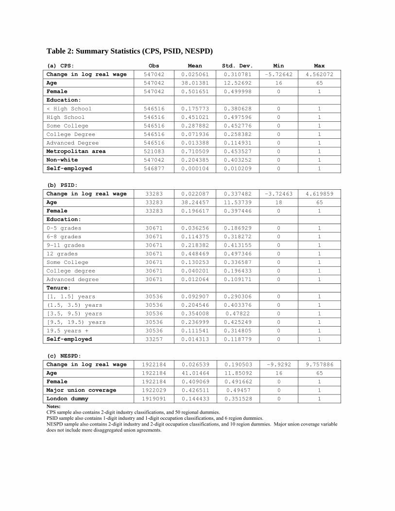
The data used in this analysis are taken from the Current Population Survey (CPS) and the
Panel Study of Income Dynamics (PSID) for the US, and the New Earnings Survey Panel Dataset
(NESPD) for Great Britain. For all datasets, the relevant wage measure used in this study is the
basic hourly wage rate for respondents aged 16 to 65. Since the CPS and PSID are relatively
well-known datasets, I only describe them brie�y here.
The CPS samples are taken from the Merged Outgoing Rotation Group (MORG) �les from 1979
to 2002. I link respondents across consecutive years using a method similar to that advocated by
Madrian & Lefgren (1999)20. This method yields approximately 25,000 individual annual wage
changes each year from 1980�2002, although changes in sampling method yield lower sample sizes
in 1985�86 and 1995�96 (see Table 1). Unfortunately, one cannot easily di¤erentiate between
job-stayers and changers using the CPS due to a lack of information on job characteristics and
tenure21. Additional problems arise in the CPS resulting from the survey redesign in 1994. Figure
8 illustrates the dispersion of log wage changes in the CPS over the sample period, as measured by
the standard deviation, and the 90-10 and 80-20 percentile di¤erentials. One can clearly detect
a signi�cant rise in the dispersion of wage changes starting in 199422. In the ensuing empirical
analysis I attempt to control for this.
The PSID data are taken from the random (not poverty) samples for the years 1971 to 1992.
I use data on regular hourly pay rates for household heads to construct individual annual wage
changes. I concentrate on the wage changes of job-stayers23 by excluding workers with tenure of20 In particular, �rst we match individuals according to their personal identi�ers, as well as their month of interview.
We then employ Madrian & Lefgren�s �sjrja� criterion � i.e. that matched observations must report the same sexand race across years, and that the di¤erence in their age must lie in the interval [0; 2].21Card & Hyslop (1997) attempt to identify job-stayers in the CPS by restricting their analysis to those respondents
who do not change occupation year-on-year. We do not make such an attempt as it is complicated by changes in theoccupational classi�cation over the period. However, the sample used in this paper displays very similar propertiesto that of Card & Hyslop.22This is likely to be due in particular to an increase in the fraction of imputed wage observations in the CPS for
1994 onwards. However, it is di¢ cult to simply deleted such imputed observations from the analysis due to largechanges in the accuracy of the CPS imputation �ags over the period �see Hirsch & Schumacher (2004).23 It should be noted that tenure in the PSID refers to the time spent with the same employer, except for the years
1979�80 when it refers to the time spent in the same position.
21
strictly less than 12 months24, and additionally remove respondents who report that they live in
a foreign country, and top-coded wage data. The PSID sample provides us with much smaller
samples than those from the CPS, with approximately 1,300�2,200 individual wage changes each
year over the sample period (see Table 1).
Finally, the NESPD is an individual level panel which is collected in April of each year running
from 1975 through to 2001 for Great Britain25. It is a 1% sample of British income tax-paying
workers with a National Insurance (Social Security) number that ends in a given pair of digits. The
wage measure used is the gross hourly earnings, excluding overtime, of job-stayers whose pay is
una¤ected by absence. Table 1 provides summary statistics for the NESPD sample. An important
observation to make is that the statistics for the level of real wage growth in 1977 are vastly lower
than in all other periods in the NESPD. In particular, the fraction of respondents reporting a real
wage cut was 77:64% in 1977, but was never below 52% in any other year in the sample period (see
Table 1). The reason for this is that the UK government of the time instituted an incomes policy
in order to try to curb high in�ation. In particular, these policies were remarkably successful in
containing wage in�ation in late 1976 to early 1977 as a result of the cooperation of the unions
(see Cairncross, 1995, pp. 220�221). Despite this, however, retail price in�ation remained high,
thereby leading to the signi�cant real wage losses that I observe in the data. As a result of this, I
treat the 1977 data as an outlier throughout the rest of the analysis.
Since the descriptive properties of DNWR in all of these datasets have been well-explored in
previous analyses � Card & Hyslop (1997) for the CPS, Kahn (1997) and Altonji & Devereux
(2000) for the PSID, and Nickell & Quintini (2003) for the NESPD �I do not seek to provide a full
descriptive account of DNWR. For reference, though, Tables 1 and 2 present summary statistics
for wage changes and the key variables that will be used in the forthcoming analysis. The primary
aim of the current section is rather to assess the validity of the predictions of the model presented
24A selection issue arises when excluding job-changers. In particular, previous research has shown that �displaced�workers often accept signi�cant reductions in earnings on re-employment (see Jacobson, LaLonde & Sullivan, 1993).Thus, by concentrating on job-stayers, our results might overstate the true extent of DNWR. However, it is also thecase that much of the previous literature has focused on job-stayers, so our analysis will be comparable to that ofother studies. We leave these empirical issues for future research.25However, much of our analysis requires the use of consistent industry and occupation coding, which we have up
to 1999 only.
22
in section 2. However, it should be noted that the NESPD data for Great Britain have a number
of key advantages for the purposes of this paper, especially in comparison with the CPS and PSID
samples for the US.
The �rst, and most obvious, is that the NESPD provides us with comparatively very large
sample sizes: one obtains sample sizes of 60�80,000 wage change observations each year. The
second advantage of the NESPD data is its sample period: from 1975�2001. This is particularly
useful given that I seek to use variation in the rate of in�ation to gauge the impact of DNWR on
wage changes, since the UK experienced signi�cant variation in in�ation over this period relative
to the US. Figure 9 displays the time-series of the leading UK in�ation indicator �the Retail Price
Index (RPI) �and the CPI-U in�ation rate for the US, over the relevant periods. It can be seen
that the UK in�ation rate varied substantially, with rates over 20% in the 1970s down to below 2%
in the 1990s. In�ation in the US, on the other hand, displays much less variation, with rates no
higher than 11%.
The �nal key advantage of the NESPD sample is that measurement error in these data is likely
to be less of a problem relative to individually reported data of the CPS and PSID samples. The
reason for this is that the NESPD is collected from employers�payroll records, thereby leaving less
scope for error due to imperfect memory etc. (see Nickell & Quintini, 2003, for more on this)26.
This is important because the existence of measurement error in hourly wages has been shown
in previous empirical studies to act as a key impediment to inferring the extent of DNWR. As
emphasized throughout this analysis, the existence of a spike at zero in the distribution of nominal
wage changes is a key characteristic of DNWR. Classical measurement error in wages and hours
data would yield an understatement of the spike by rendering true wage freezes to be observed
as (small) wage changes (Akerlof et al., 1996). In contrast, previous studies have also stressed
that individuals may round their reported wages yielding an overstatement of the extent of DNWR
as small true wage changes are reported as wage freezes (Smith, 2000). Whilst some existing
studies have attempted to circumvent this by explicitly modelling measurement error, or using
26 Indeed validation studies of leading panel datasets have used matched data from employer surveys to assess theextent of measurement error in worker reported earnings data. In particular, Bound & Krueger (1990) and Card &Hyslop (1997) both seek to assess the importance of measurement error in the CPS via this method.
23
data from payroll records of individual establishments (Altonji & Devereux, 1999; Fehr & Goette,
2003), the relative accuracy of the NESPD allows us to avoid these di¢ culties and preserve a more
representative sample, and is thus an important virtue in this context27.
A �nal note worth making in the context of these datasets is that in�ation stayed at persistently
low levels in the US and UK from 1992 onwards, with an average in�ation rate of 2.56% for the US
1992�2002 and 2.69% for the UK 1992�2001. This is important, as a criticism levelled at previous
studies of DNWR has been that individuals will get used to receiving nominal wage cuts when
in�ation has remained low for some time (Gordon, 1996, and Mankiw, 1996). Such a criticism
becomes less compelling when the in�ation rate has stayed low for the 9�10 years observed in the
samples for the CPS and the NESPD.
4.2 Does DNWR Increase Aggregate Wage Growth?
In order to test the hypotheses of section 3, one needs a way of modelling empirically the wage
change distribution, f (� lnW ). In what follows, I will focus on the analogous real wage change
distribution counterpart to this28. In order to motivate my preferred method, let us begin by
considering some naive approaches. First, one might think of simply looking at the di¤erences
between the wage change distributions in high in�ation periods and low in�ation periods to see if
the predictions of section 3 are con�rmed at this basic level. To this end, �gures 10(a) and 11(a)
present estimates of the density of log real wage changes for periods with di¤erent in�ation rates
using the PSID for the US, and the NESPD for Britain (the redesign of the CPS renders this a less
useful exercise for the CPS data). Notice that lower in�ation leads to a compression of the lower
and, more importantly for our purposes, the upper tail of the wage change distribution, precisely
in accordance with the predictions of section 4.129.
27 It should be noted that hourly earnings in the NESPD are derived from dividing weekly earnings by weeklyhours, thereby potentially exacerbating any underlying measurement error. However, Nickell & Quintini (2003) havecompared the accuracy of hourly wage changes in the NESPD with those obtained from a sample whose payslip waschecked in the British Household Panel Study and found remarkably similar properties in both datasets.28Note that this does not alter any substantive aspects of the analysis, since this is exactly the same shaped
distribution, just shifted to the left by a constant, �ln (W=P ) = � lnW ��lnP �= � lnW �� where � is the rate ofin�ation. However, focusing on real wage changes does allow greater ease of comparison across years with di¤erentin�ation rates.29 It should be noted that the existence of the spike in the lower tail of the real wage change distribution (at
approximately minus the rate of in�ation) can lead to an overstatement of lower tail compression. However, our
24
However, one could argue that at least some of the observed di¤erences were due to changes in
other variables that a¤ect wage changes. For example, there have been changes in the industrial,
age, gender, regional etc. compositions of the workforce in both the US and Britain over these
time periods. So, one should control for factors such as these before attributing any di¤erences
to DNWR. To address this, I introduce a set of micro-level control variables for each dataset,
summarized in Table 2. In particular, I control for changes in micro-level variables by re-weighting
the observed wage change distributions according to the method of DiNardo, Fortin & Lemieux
(1996) (henceforth DFL)30. To do this, I �rst de�ne a �base year�, T �for all datasets this will
be the �nal sample year �and re-weight each year�s observed wage change distribution to obtain
an estimate of what the wage change distribution would have looked like if the distribution of
micro-level characteristics were identical to that at date T . In particular, if one de�nes the log
wage change as �w, micro-level characteristics as x, and the year of the relevant x distribution as
tx, one can derive that:
f (�wt; tx = T ) =
Zf (�wjx) dF (xjtx = T ) =
Zf (�wjx) � � dF (xjtx = t) (16)
for all t < T . The key insight of DFL is that this is simply a re-weighted version of the observed
date t wage change distribution, with weights given by:
=dF (xjtx = T )
dF (xjtx = t)=Pr (tx = T jx)Pr (tx = tjx) �
Pr (tx = t)
Pr (tx = T )(17)
where the second equality follows from Bayes�Rule. The conditional probabilities in (17) can then
be estimated simply via a probit model.
Figures 10(b) and 11(b) displays density estimates of the DFL re-weighted distribution of log
real wage changes for di¤erent in�ation periods, again for the PSID and NESPD. Again, it can be
seen clearly that lower rates of in�ation are associated with a compression both of tails of the wage
change distribution, in line with the predictions of section 3.
emphasis is on the e¤ects on the upper tail, which are not subject to this problem.30An important bene�t of the DFL methodology is that it requires few parametric assumptions on the impact of
the x variables. Given the intrinsically non-linear character of the wage policy (13), this is especially helpful.
25
However, even having controlled for such factors, it is still not necessarily legitimate to attribute
all the residual di¤erence in the wage change distributions to DNWR. Thus we need a way
of ensuring that only the variation in wage change distributions that varies systematically with
DNWR is attributed. To do this, I estimate regressions of the form:
Pnrt = �0n + �1nP50rt + �n�t + z0rt n + "nrt (18)
where Pnrt is the nth percentile of the real wage change distribution in region r at time t, �t is the
rate of in�ation at time t and thereby measures the prominence of nominal zero in the distribution
of log real wage changes, and zrt is a vector of aggregate controls that could potentially a¤ect the
distribution of wage changes. P50rt is included on the RHS of (18) in order to control for changes in
the central tendency of the distribution of wage changes. That is, it �re-centres�the distributions
over time in order to make them comparable. I estimate (18) by Least Squares, where I weight by
the size of the region at each date31.
The measure of in�ation used will be the CPI-U-X1 series for the US, and the April to April
log change in the Retail Price Index for Great Britain. The aggregate controls will be as follows.
First, I control for any distortion to the wage change distributions caused by peculiarities of the
datasets used. So, to control for the e¤ects of survey redesign issues after 1994 in the CPS, I
include a dummy variable that takes value one for all years from 1994 onwards when I estimate
(18) for the CPS. In addition, to control for the incomes policies implemented in 1977 in the UK,
I include a dummy that takes value one for the year 1977 in the NESPD regressions.
In addition, I control for the absolute change in the rate of in�ation. This is motivated by the
hypothesis that greater in�ation volatility will yield greater dispersion in relative wages regardless
of the existence of DNWR (see Groshen & Schweitzer, 1999). I also include both current and
lagged regional unemployment rates. This is motivated by the idea that the existence of DNWR
might lead to unemployment � indeed, as mentioned before, this is one of the principal reasons
31Formal quantile regression (Least Absolute Deviation) estimators were also tried with little di¤erence in results.However, such is the computational intensity involved in estimating the correct standard errors for these estimators,we opted for simple OLS instead.
26
for interest in the topic. Since unemployment will lead to workers �leaving� the wage change
distribution, it is important to control for any resulting distributional consequences. I also include
lagged regional unemployment in accordance with the wage curve hypothesis of Blanch�ower &
Oswald (1994) that the level of wages is empirically associated with the level of unemployment. If
this is true, then one would expect the change in unemployment to a¤ect the change in wages, and
so I include lagged regional unemployment to control for this possibility.
It should be noted that the empirical method described above is robust to a number of possible
concerns. First, the speci�cation is robust to the existence of rigidity in real wages. The reason
is that real wage rigidity, in its traditional form, will be invariant to in�ation by de�nition. An
exception to this is the argument put forward by Akerlof, Dickens & Perry (2001) that real wage
rigidity is ampli�ed as in�ation rises because it becomes optimal for workers to direct their scarce
attention to maintaining their real wage. However, if anything, such a possibility would work
against the claim of the model in section 2, as it would predict that the upper tail of wage changes
would become more compressed as in�ation rises. If this were the case, any evidence I �nd for
the predictions of section 3 could be interpreted as lower bounds on the true e¤ects. A similar
reasoning applies to any concerns one might have about the impact of skill-biased technical change
(SBTC). Under SBTC, one might expect that workers obtaining high wage increases early in these
samples will obtain even higher wage increases later on as technical change increasingly favors those
in skilled sectors. However, since in�ation is in practice declining over the sample periods of the
data, SBTC would, if anything, work against the predictions of section 3.
Clearly, the coe¢ cients of interest in (18) for the purposes of estimating the e¤ects of DNWR
are �n. In particular, the predictions of section 3.2 indicate that �n should be negative for low
percentiles, and positive for high percentiles. The reasoning is that higher in�ation should lead to
an increased dispersion of wage changes, and thereby decrease negative percentiles, and increase
positive ones.
Recall that we would like to obtain an estimate of the increase in average wage growth due to
DNWR, � � E (�wjDNWR)�E (�wjno DNWR). Such an estimate can be obtained using the
estimates obtained from regressions of the form (18). In order to use this information to get an
27
estimate of �, I obtain an estimate of the predicted average wage change when in�ation is very low
(e.g. 1.3% in 1993 for Britain) and subtract the analogous average wage change when in�ation is
very high (e.g. 21.8% in 1980 for Britain)32:
� = E (�wj� = 1:3%; x; z)� E (�wj� = 21:8%; x; z) (19)
To obtain these estimates using (18), one can use the fact that the quantiles of a random variable
are uniformly distributed. In particular, if one estimates k equi-spaced percentiles of f (�w) then
a best guess of the predicted average wage change is:
E (�wj�; x; z) � 1
2 (k � 1)
k�1Xi=1
�Pi + Pi+1
�(20)
where i is an ascending index of the percentiles, with i = 1 indicating the lowest percentile, i = 2
the second lowest etc., and the P s are the predicted values of these percentiles obtained from
estimating equation (18).
Since these predicted percentiles allow us to sketch out a discretization of the whole distribution
of wage changes, I can also decompose the increase in average wage growth due to DNWR into two
components. The �rst is the increase in average wage growth due to compressed nominal wage
cuts, which I refer to as �lower tail losses�; the second is the decrease in average wage growth due
to compressed wage increases, �upper tail gains�. In practice, I will perform this procedure on 99
estimated wage change percentiles, P1; P2; :::; P99, for the speci�cation detailed above.
The E¤ects of Measurement Error
As mentioned previously, the impact of measurement error on the ability to infer the e¤ects of
DNWR has received substantial attention in the literature. Whilst I have attempted to mitigate
this as a problem by using the relatively clean data in the NESPD for Britain, the question arises
as to the e¤ects of measurement error on the methodology detailed above. Proposition 7 answers
this question:
32Note that this involves out-of-sample predictions for the US data.
28
Proposition 7 If measurement error is independent of the rate of in�ation, then (i) estimates of �n
in (18) report attenuated estimates of the corresponding true e¤ects; (ii) this attenuation vanishes
for su¢ ciently high and low percentiles; and (iii) estimates of � based on (20) will nonetheless
remain consistent.
The intuition for this is quite straightforward33. The existence of measurement error will render
some true negative wage changes to be observed as positive wage changes (and vice versa). Thus,
measurement error will lead to a partial con�ation of the e¤ects of in�ation on the upper tail
with those in the lower tail. However, as one proceeds further into the tails of the wage change
distribution, the likelihood of measurement error having displaced observations in this way becomes
smaller. Thus, such attenuation will disappear for su¢ ciently high or low percentiles.
Whilst this result does mean that a certain caution should be a¤orded to the interpretation
of the magnitude of the estimated coe¢ cients from (18), the main question under discussion is a
qualitative one: does lower in�ation compress both the upper and lower tails of the wage change
distribution? To this end, the above attenuation result will actually reduce the ability to observe
any such compression, should it exist. Thus, any evidence of compression that might be found
would be found despite the existence of measurement error, rather than because of it.
The �nal part of Proposition 7 results from the fact that, by de�nition, the mean of any random
variable can always be expressed as an unweighted average of its percentiles. Since measurement
error is assumed independent of the rate of in�ation (see Gottschalk, 2004, for evidence that this is
empirically the case), it follows that the observed mean wage change at any given rate of in�ation
will be una¤ected by the existence of measurement error. Thus, estimates of � based on (20)
should also be una¤ected by measurement error.
Empirical Results
I estimate (18) in three speci�cations. First, I simply include controls for the median wage change,
P50, and for any dataset peculiarities such as the CPS survey redesign from 1994 onwards and
33 It should be noted, however, that this attenuation result is quite distinct from the traditional attenuation biasresulting from errors in variables when implementing OLS.
29
incomes policies of 1977 in the NESPD. I then include controls for the absolute change in the
rate of in�ation, and for regional current and lagged unemployment rates. Finally, I implement a
speci�cation with full controls that estimates (18) using percentiles of the DFL re-weighted wage
change distributions so I can control for an array of micro-level characteristics as well.
The results from estimating the three speci�cations of (18) for each dataset are reported in
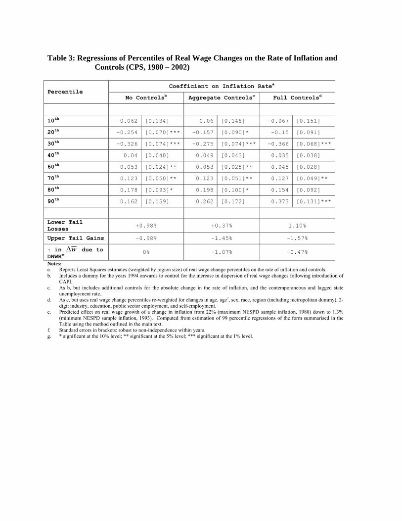
Tables 3�5. First, consider the results obtained for the CPS in Table 3. In all three speci�cations
it can be seen that the estimated impact of in�ation is negative for the 20th�30th percentiles, with
strongest e¤ects around the 30th percentile; and positive for the 40th�90th percentiles, with strong
e¤ects in the 60th�90th percentiles. Thus, these results are in line with the hypothesis that higher
in�ation reduces the compression of both tails of the wage change distribution. Moreover, it can
be seen that the estimated e¤ects of in�ation at di¤erent points in the distribution are generally
signi�cant and fairly stable across all speci�cations. In addition, Table 3 presents estimates of the
lower tail losses and upper tail gains due to DNWR. It can be seen that in all speci�cations there
are substantial savings due to compressed wage increases, some of which even outweigh the costs
from compressed wage cuts.
Table 4 reports the analogous estimates for the PSID data. It can be seen that in all speci�ca-
tions the e¤ect of in�ation is negative for the 10th�20th percentiles, and positive for the 40th�90th
percentiles. However, here the estimated e¤ects are strongest in the 10th, and particularly the
20th, percentiles in the lower tail in contrast to the CPS results. The di¤erences in the lower tail
e¤ects between the CPS and PSID results are likely to re�ect the di¤erences in the position of nom-
inal zero in the respective wage change distributions, due to higher rates of in�ation in the PSID
sample period. In the CPS, nominal zero appears mostly between the 20th and 35th percentiles,
whereas it appears at around the 10th�35th percentile in the PSID sample. Thus, the point at
which DNWR binds di¤ers across these two datasets.
The PSID results are broadly as signi�cant as those for the CPS, with both lower and upper
tail e¤ects remaining signi�cant, and fairly stable across speci�cations. In addition, the coe¢ cient
estimates in the upper tail are comparable to those obtained in the CPS results, and one again can
observe that there are large savings from the compression of the upper tail. In particular, I �nd
30
an estimated increase in average wage growth due to lower tail losses of around 1 � 1:2% which
is o¤set by a reduction in average wage growth due to upper tail compression of 0:9 � 1:1%. It
should however be noted that for the PSID, and to some extent the CPS data, these estimates
are constructed from a number of regressions for which no signi�cant in�ation e¤ect was detected.
This is likely due to the relative lack of observations and in�ation variation in the CPS and PSID
compared to the NESPD. Thus, I do not want to place too much stock in the actual quantitative
estimates obtained from this dataset. Rather, I consider the estimates of upper tail gains and lower
tail losses for the PSID to be instructive of the fact that there is some signi�cant compression of
the upper tail of wage changes, and that this compression is of similar signi�cance and magnitude
to the compression of the lower tail due to DNWR.
The results for the NESPD data are reported in Table 5. Again I observe that in�ation has
a negative impact on lower percentiles (10th�40th) and a positive impact on higher percentiles
(60th�90th). Moreover, I obtain highly signi�cant estimates for almost all percentiles and in all
speci�cations. As mentioned above, this greater signi�cance in comparison to the results for the
PSID and the CPS is likely to be due to the larger sample sizes, more precise wage information, and
large variation in in�ation in the NESPD. In addition, one can again observe substantial upper tail
gains due to compression of wage increases relative to lower tail losses, which are more consistent
across speci�cations than those obtained for the CPS and the PSID. In particular, the results
suggest that 75�95% of the lower tail losses due to DNWR is saved by restricting wage increases
in the upper tail in the NESPD data, and that the increase in average real wage growth due to
DNWR is of the order 0.04�0.3% �much lower than results obtained previously.
Together, these results provide strong evidence for the prediction that the upper tail of the wage
change distribution will be less dispersed as a result of DNWR �in all speci�cations and for all
datasets one can see that wage increases become more restricted as in�ation falls. As a result, by
allowing both the upper and lower tails of the wage change distribution to be a¤ected by DNWR,
the estimated increase in average wage growth due to DNWR becomes much reduced and closer to
zero �precisely in line with the predictions of section 3 and Proposition 5.
31
4.3 Does Higher Turnover Reduce the Compression of Wage Increases?
In addition to the above, recall that section 3.3 established the claim that higher turnover sectors
should act more myopically, will thus feel more at liberty to raise nominal wages, but that such an
e¤ect should fade as in�ation rises34. I test this hypothesis in a manner similar to that employed
in section 4.2. First, I de�ne a measure of �turnover�as the fraction of workers that changes jobs
each year in a given occupation, region group. In a steady state this should closely match the
fraction of workers who separate, and thus correspond to the parameter � in section 3.3.
To gain an initial impression for whether such e¤ects exist, Figure 12(a) plots density estimates
of the nominal wage change distribution for job stayers in high and low turnover (respectively above
and below median turnover) occupations using the NESPD data35. It can be seen from this simple
comparison that low turnover occupations seem to be compressing wage increases much more than
high turnover occupations.
However, recall that section 3.3 noted that these e¤ects should be manifested through changes
in the active compression of wage increases, and thus relate to the properties of the conditional
distribution, f (� lnW jW�1). To address this issue, Figure 12(b) replicates the exercise but
controls for the covariates listed in Table 2, as well as the lagged wage36, using the DFL technique.
This allows us to control for any micro-level factors that may be driving the results, as well to
focus on variation in the distribution of wage changes conditional on the lagged wage. Again,
however, one can see low turnover occupations compressing wage increases more than high turnover
occupations, consistent with the predictions of section 3.3.
To complete the picture, panels (c) and (d) of Figure 12 attempt to assess whether the e¤ect of
turnover on the distribution of wage changes varies with the rate of in�ation. It can be seen that
34Note that we are making a claim about the e¤ects of turnover on the distribution of wage growth rather thanmean wage growth. Clearly, there are additional concerns that would relate turnover to mean wage growth suchas e¤ects on tenure, match quality etc. These are not however related to compression of the distribution of wagegrowth emphasized here.35Since tenure is not reported in the CPS, and is subject to changes in de�nition in the PSID, we concentrate on
the NESPD data for this section.36 In particular, we use the lagged wage adjusted for in�ation and productivity growth, ~Wt�1 �Wt�1 � PT�1Pt�1
� aT�1at�1
,where as is measured as GDP per hour in year s. This is legitimate provided that DNWR has no impact on eitherprice or productivity growth. Given Proposition 5 and the results of section 4.2 this does not seem unreasonable.
32
the compression of wage increases due to lower turnover appears to be stronger in periods of low
in�ation, as predicted by the model of section 2. Together, then, there appears to be suggestive
evidence that the predictions of section 3.3 are supported in the data.
To identify these turnover e¤ects more formally, however, I run Least Squares regressions of the
where Pnort now refers to the nth percentile of nominal wage changes for job stayers, re-weighted for
micro covariates and the lagged wage, in occupation o, region r, at time t. The variable of interest
is � ort which denotes the fraction of job changers in an occupation, region, year cell. Under the
predictions of section 3.3, one would expect that the coe¢ cients on turnover, �n, to be positive,
the coe¢ cients on in�ation, �n, to be positive, and the coe¢ cients on the interaction term, �n, to
be negative, for all positive percentiles of nominal wage changes.
Table 6 summarizes these estimates for the 60�90th percentiles. In the �rst speci�cation
(column 1), I include only basic controls for the median wage change and a dummy for 1977 to
control for the incomes policies of that time, and exclude the rate of in�ation and its interaction
with turnover. It can be clearly seen that turnover has a positive and highly signi�cant impact on
the 60�90th percentiles of nominal wage changes. The two additional columns address potential
concerns one might have about the simple speci�cation of column (1).
In particular, one concern might be that one would expect sectors with greater DNWR to have
greater rates of turnover due to workers being made unemployed more often. In addition, one
would also expect sectors with greater DNWR to exhibit a greater compression of wage increases,
and thus create downward pressure on percentiles of wage increases. In this sense there may be
an omitted variable �the extent of DNWR �that will lead to bias in the estimates of column (1).
In particular, it would imply a downward bias to the estimates. Column (2) seeks to assess this
possibility by including the current and lagged regional unemployment rates as controls. It can
be seen, however, that this actually reduces the estimated e¤ects of turnover, which nevertheless
remain positive and highly signi�cant. Thus, there does not appear to be strong evidence for an
33
omitted variables problem of this type.
However, one may still be concerned that the measure of turnover is more generally cyclical,
and thus potentially correlated with the rate of in�ation. Thus one may be worried that the
above results are attributing to turnover the e¤ects due to declining in�ation. One may also be
concerned that the e¤ects of in�ation found in section 4.2 are not robust to the addition of turnover
as a control. Finally, one would like to assess whether the e¤ect of turnover on the distribution
of wage changes diminishes as in�ation rises. To address these concerns, speci�cation (3) includes
the rate of in�ation and the interaction between in�ation and turnover as regressors. It can be
seen that introducing these controls does not signi�cantly alter the estimated e¤ects of turnover,
and that the coe¢ cients remain positive and highly signi�cant. Moreover, I �nd that the e¤ect
of in�ation is robust to the addition of turnover as a control, and remains positive and highly
signi�cant for all except the 90th percentile of wage changes.
The coe¢ cients on the interaction between turnover and in�ation are less successful, however.
In particular, the estimates are positive, but close to zero and highly insigni�cant for the 60th and
70th percentiles. The estimates for the 80th and 90th percentiles are negative and much larger
in magnitude � in accordance with the �behavioral� model�s predictions � though the e¤ect is
signi�cant only at the 80th percentile. However, these latter estimates imply that a 20% in�ation
rate will reduce the e¤ect of turnover on the distribution of wage changes by 50�60%.
I thus �nd robust evidence that increased turnover leads to an increased dispersion of wage
increases, that the e¤ects of turnover and in�ation are mutually robust, and that there is sugges-
tive evidence that the e¤ects of turnover are reduced as in�ation rises, broadly in line with the
predictions of section 3.3.
5 Conclusions
This paper has shown that a model of allocative downward nominal wage rigidity driven by worker
resistance to nominal wage cuts is nevertheless consistent with weak macroeconomic e¤ects. It
has shown as a theoretical issue that DNWR should have no e¤ect on aggregate wage growth in
34
the long run, and that this is achieved because �rms compress wage increases as well as wage cuts
when DNWR binds. Moreover, it has shown that, by neglecting potential compression of wage
increases, the previous literature may well have overstated the increase in aggregate wage growth
due to DNWR, and thereby substantially overstated the costs of DNWR to �rms.
Taking these predictions to a broad range of micro�data on wages from the US and Great
Britain I �nd that �rms do indeed compress wage increases as well as wage cuts at times when
DNWR binds. Furthermore I �nd that accounting for the compression of wage increases reduces
the estimated increase in aggregate wage growth due to DNWR to be much closer to zero, consistent
with the predictions of the model. Together, the results suggest that the existence of DNWR may
not provide a strong argument against the targeting of low in�ation rates, as practiced by many
monetary authorities. Importantly, though, this result is nevertheless consistent with the wide
array of evidence that suggests workers are averse to nominal wage cuts.
Stepping back from this, one might ask whether the key mechanism put forward in this paper
� that �rms may compress wage increases in the face of DNWR � really rings true in the real
world. There is, in fact, subjective evidence that wage setters and workers do think along these
lines. Following his original study (Bewley, 1999), Bewley has since reported that:
�[Business leaders] take account of the fact that, if they raise the level of pay today,
it will remain high in the future. I hear a lot about this last point now. [...] Some say
that they are not now increasing pay [...] because they know they will not be able to
reverse the increases during the next downturn.� Bewley (2000), p.46.
In addition, there is evidence of explicitly bargained mediation of wage growth as an alternative to
wage cuts:
�General Motors Corp�s historic health care deal with the United Auto Workers will
require active workers to forgo $1-an-hour in future wage hikes [...] Allen Wojczynski, a
36-year GM employee, said the company�s proposal seems acceptable [...] He had been
expecting the automaker to ask its workers for pay cuts to trim health care costs. �I
35
could live with it, giving up $1 an hour of my future pay raises,�said Wojczynski [...]�
Detroit News, October 21st 2005.37
Thus, compression of wage raises is a practical approach to limiting labor costs in the face of poor
economic conditions, and can thereby limit disemployment e¤ects of worker resistance to wage cuts.
6 References
Abel, Andrew B., and Janice C. Eberly, �Optimal Investment with Costly Reversibility�, Reviewof Economic Studies, Vol. 63, No. 4. (Oct., 1996), pp. 581-593.
Akerlof, George A., William T. Dickens, and George L. Perry, �The Macroeconomics of Low In�a-tion�, Brookings Papers on Economic Activity, Vol. 1996, No. 1. (1996), pp. 1-76.
Akerlof, George A., William T. Dickens, and George L. Perry, �Near Rational Wage and PriceSetting and the Long-Run Phillips Curve�, Brookings Papers on Economic Activity, Vol. 2000, No.1. (2000), pp. 1-44.
Akerlof, George A., and Janet L. Yellen, E¢ ciency Wage Models of the Labor Market, CambridgeUniversity Press, 1986.
Altonji, Joseph & Paul Devereux, �The Extent and Consequences of Downward Nominal WageRigidity�, Research in Labor Economics, Vol 19, Elsevier Science Inc. (2000): 383-431.
Barro, Robert J., �Long-Term Contracting, Sticky Prices, and Monetary Policy,�Journal of Mon-etary Economics, 3, (1977), 305�316.
Bentolila, Samuel, and Giuseppe Bertola, �Firing Costs and labor Demand: How Bad is Euroscle-rosis?�, Review of Economic Studies, Vol. 57, No. 3. (Jul., 1990), pp. 381-402.
Bewley, Truman F., Why wages don�t fall during a recession, Cambridge and London: HarvardUniversity Press, 1999.
Bewley, Truman F., Comment on Akerlof, George A., William T. Dickens, and George L. Perry,�Near Rational Wage and Price Setting and the Long-Run Phillips Curve�, Brookings Papers onEconomic Activity, Vol. 2000, No. 1. (2000), pp. 1-44.
Blanch�ower, David G., Andrew J. Oswald, The Wage Curve, Cambridge and London: MIT Press,1994.
Bloom, Nicholas, �The Real Options E¤ect of Uncertainty on Investment and labor Demand�, IFSWorking Paper, November 2000.37See http://www.detnews.com/2005/autosinsider/0510/21/A01-356532.htm. This is not to claim that the latter
agreement is the key solution to this particular labor con�ict; just that it is indicative that the results of this paperbear some resemblance to wage setting in the real world.
36
Cairncross, Alec, The British Economy since 1945, 2nd edition, Blackwell, 1995.
Card, David & Dean Hyslop �Does In�ation �Grease the Wheels of the Labor Market�?�in ChristinaD. Romer and David H. Romer, editors, Reducing In�ation: Motivation and Strategy. Universityof Chicago Press, 1997.
DiNardo, John, Nicole M. Fortin, and Thomas Lemieux, �Labor Market Institutions and the Dis-tribution of Wages, 1973-1992: A Semiparametric Approach�, Econometrica, Vol. 64, No. 5. (Sep.,1996), pp. 1001-1044.
Dickens, William T., Lorenz Goette, Erica L. Groshen, Steinar Holden, Julian Messina, Mark E.Schweitzer, Jarkko Turunen, and Melanie Ward, �The Interaction of Labor Markets and In�a-tion: Analysis of Micro Data from the International Wage Flexibility Project,�mimeo BrookingsInstitution, 2006.Fehr, E. & L. Götte, �Robustness and Real Consequences of Nominal Wage Rigidity,�Institute forEmpirical Research in Economics, University of Zürich, Working Paper No. 44.
Genesove, David & Christopher Mayer, �Loss Aversion and Seller Behavior: Evidence from theHousing Market�, Quarterly Journal of Economics. November 2001; 116(4): 1233-60.
Gordon, R., Comment on: Akerlof, George A., William T. Dickens, and George L. Perry, �TheMacroeconomics of Low In�ation�, Brookings Papers on Economic Activity, Vol. 1996, No. 1.(1996), pp. 1-76.
Gottschalk, Peter, �Downward Nominal Wage Flexibility: Real or Measurement Error?�, IZA Dis-cussion Paper no. 1327, October 2004.
Groshen, Erica L.,and Mark E. Schweitzer, �Identifying In�ation�s Grease and Sand E¤ects in theLabor Market�, Feldstein, Martin, ed. The costs and bene�ts of price stability. NBER ConferenceReport series. Chicago and London: University of Chicago Press, 1999; 273-308.
Hirsch, Barry T., and Edward J. Schumacher, �Match Bias in Wage Gap Estimates Due to EarningsImputation�, Journal of Labor Economics, 2004, vol. 22, no. 3.
Howitt, Peter, �Looking Inside the Labor Market: A Review Article�, Journal of Economic Liter-ature 40 (March 2002): 125-38.
Jacobson, Louis S., Robert J. LaLonde, and Daniel G. Sullivan, �Earnings Losses of DisplacedWorkers�American Economic Review, Vol. 83, No. 4. (Sep., 1993), pp. 685-709.
Kahn, Shulamit, �Evidence of Nominal Wage Stickiness from Microdata�, American EconomicReview, Vol. 87, No. 5. (Dec., 1997), pp. 993-1008.
Kahneman, Daniel, Jack L. Knetsch, and Richard Thaler, �Fairness as a Constraint on Pro�tSeeking: Entitlements in the Market�, American Economic Review, Vol. 76, No. 4. (Sep., 1986),pp. 728-741.
Kahneman, Daniel, and Amos Tversky, �Prospect Theory: An Analysis of Decision under Risk�,Econometrica, Vol. 47, No. 2. (Mar., 1979), pp. 263-292.
37
Keynes, John Maynard, The General Theory of Employment, Interest, and Money, 1936.
Kramarz, F., �Rigid Wages: What Have we Learnt from Microeconometric Studies�, in Advancesin Macroeconomic Theory, J. Drèze ed., 194-216, Oxford University Press, Oxford, UK.
Lebow, David E., Raven E. Saks, Beth-Anne Wilson, �Downward Nominal Wage Rigidity: Evidencefrom the Employment Cost Index�, Board of Governors of the Federal Reserve System, Financeand Economics Discussion Series: 99/31 July 1999.
Madrian, Brigitte, and Lars J. Lefgren, �A Note on Longitudinally Matching Current PopulationSurvey (CPS) Respondents�NBER Technical Working Paper 247, November 1999.
Mankiw, N. G., Comment on: Akerlof, George A., William T. Dickens, and George L. Perry, �TheMacroeconomics of Low In�ation�, Brookings Papers on Economic Activity, Vol. 1996, No. 1.(1996), pp. 1-76.
Nickell, S., and Glenda Quintini, �Nominal wage rigidity and the rate of in�ation�, EconomicJournal, October 2003, vol. 113, no. 490, pp. 762-781(20).
Sha�r, Eldar, Peter Diamond, and Amos Tversky, �Money Illusion�, Quarterly Journal of Eco-nomics. May 1997; 112(2): 341-74.
Smith, Jennifer, �Nominal wage rigidity in the United Kingdom�, Economic Journal 110 (March2000), 176-195.
Smith, Jennifer, �How Costly is Downward Nominal Wage Rigidity in the UK?�, mimeo, December2004.
Solow, Robert M., �Another Possible Source of Wage Stickiness�, Journal of Macroeconomics, Vol.1, pp.79�82, Winter 1979.
Stokey, Nancy L., and Robert E. Lucas Jr., Recursive methods in economic dynamics, with EdwardC. Prescott Cambridge, Mass. and London: Harvard University Press, 1989.
Tobin, James, �In�ation and Unemployment,� American Economic Review, Vol. 62, No. 1/2.(1972), pp. 1-18.
7 Appendix
A Lemmas and Proofs
Lemma 1 The value function de�ned in (5) has the following properties:
v�W�W;A0
�= �cA
0
W(22)
v0W�W;A0
�=
A0
W� 1 + �
1 + �D�W;A0
�v+W
�W;A0
�= 0
38
Proof. First, note that standard application of the Envelope Theorem implies:
v�W�W;A0
�= c
A0
W(23)
v+W�W;A0
�= 0
It is only slightly less obvious what happens when �W 0 = 0, i.e. when the wage is not adjusted.In this case, W 0 =W and this implies that:
v0�W;A0
�= A0 ln
�W
B0
��W +
�
1 + �
Zv�W;A00
�dF�A00jA0
�(24)
It therefore follows that:
v0W�W;A0
�=A0
W� 1 + �
1 + �
ZvW
�W;A00
�dF�A00jA0
�(25)
Since, by de�nition D (W;A0) �RvW (W;A
00) dF (A00jA0), the statement holds as required.Proof of Proposition 2. First, note that one can re-write the continuation value conditional
on each of the three possible continuation regimes:
v�W;A0
�=
8<:v� (W;A0) if A0 < A0lv0 (W;A0) if A0 2 [A0l; A0u]v+ (W;A0) if A0 > A0u
(26)
where superscripts �=0=+ refer to whether the nominal wage is cut, frozen, or raised tomorrow.Note also that, due to the recursive nature of the problem:
Al � l (W�1) ; Au � u (W�1) (27)
=) A0l � l (W ) ; A0u � u (W )
Thus we can write38:Zv�W;A0
�dF�A0jA
�=
Z l(W )
0v��W;A0
�dF +
Z u(W )
l(W )v0�W;A0
�dF +
Z 1
u(W )v+�W;A0
�dF (28)
Taking derivatives with respect to W and recalling the de�nition of D (�), and noting that, sincev (W;A0) is continuous, it must be that v� (W; l (W )) = v0 (W; l (W )) and v0 (W;u (W )) = v+ (W;u (W ))yields:
D (W;A) =
Z l(W )
0v�W
�W;A0
�dF +
Z u(W )
l(W )v0W
�W;A0
�dF +
Z 1
u(W )v+W
�W;A0
�dF (29)
Finally, using the Envelope conditions in Lemma 1, and substituting into (29) we obtain (9) in themain text:
D (W;A) =
Z u(W )
l(W )
�A0
W� 1�dF�
Z l(W )
0cA0
WdF+
�
1 + �
Z u(W )
l(W )D�W;A0
�dF � (CD) (W;A) (30)
38Henceforth, �dF�without further elaboration is to be taken as �dF (A0jA)�.
39
To verify that C is a contraction mapping over the �relevant range� (to be de�ned shortly),we con�rm that Blackwell�s su¢ cient conditions for a contraction hold here (see Stokey & Lucas,1989, p.54). First, note that any values for (W;A) that render C unbounded cannot obtain underoptimality, since they will necessarily violate the conditional �rst-order condition, (6). Thus,we can restrict our attention to a subset of values for (W;A) around the optimum for which Cis bounded. This is what we de�ne as the �relevant range�. That C then maps the space ofbounded functions into itself over this range holds by de�nition. Given this, monotonicity anddiscounting are straightforward to verify. To verify monotonicity, �x (W;A) =
��W; �A
�, and take
D � D. Then note that:Z u( �W)
l( �W)D��W;A0
�dF�A0j �A
��
Z u( �W)
l( �W)D��W;A0
�dF�A0j �A
�(31)
=
Z u( �W)
l( �W)
hD( �W;A0)�D
��W;A0
�idF�A0j �A
�� 0
Since��W; �A
�were arbitrary, it thus follows that C is monotonic in D. To verify discounting, note
that:
[C (D + a)] (W;A) = (CD) (W;A) +�
1 + �a [F (u (W ) jA)� F (l (W ) jA)] (32)
� (CD) (W;A) +�
1 + �a
Since we know that �1+� < 1 it follows that C is a contraction over the relevant range. It therefore
follows from the Contraction Mapping Theorem that C has a unique �xed point over the relevantrange.
Proof of Proposition 5. Denote the counterfactual nominal wage at time t asW �t = At. We
seek the properties of the di¤erence in average wage growth between the �actual� (with DNWR)and counterfactual cases, which we de�ne as �:
�T � 1
T
t+TXs=t+1
ln
�Ws
Ws�1
�� 1
T
t+TXs=t+1
ln
�W �s
W �s�1
�(33)
=1
T
�ln
�Wt+T
W �t+T
�� ln
�Wt
W �t
��Then note that, from the optimal wage policy of the �rm, (13), it follows that the log�di¤erencebetween the actual and counterfactual wages must be bounded, ln (Wt=W
�t ) 2 [� lnu;� ln l]. Thus:
sup�T =1
T[lnu� ln l] = 1
TlnG (34)
inf �T =1
T[ln l � lnu] = � 1
TlnG
Therefore, for �nite G, limT!1 sup�T = 0 = limT!1 inf �T .Proof of Proposition 6. (i) De�ne the increase in wage growth due to DNWR in the
40
median�symmetric (MS) case as:
g �Z 0
�1xf (x) dx�
Z 0
�1xf (x) dx (35)
where f , and f are respectively the observed, and MS counterfactual log wage change densities.Further de�ne the true average cost of DNWR as C � E (v� � v) where v� denotes the truefrictionless value of a �rm. Taking a �rst order Taylor series approximation around c = 0 yields:
Cc=0� dC
dc
����c=0
� c (36)
Note �rst that dC=dcjc=0 = ��@v@c +
@v@W � @W@c
���c=0
= �EP1t=0 �
tat� lnAt1�t = �E (� lnA1�)
E(a)1�� ,
since @v=@W jc=0 = 0, and where the second equality follows from the stationarity of, and the in-dependence of increments to, the shock process. It follows from this that the costs of DNWR areentirely driven by reductions in e¤ort following wage cuts. Next, note that by using the de�nition
of G in (55) one can show that lnGc=0� c.
The �nal step for part (i) is to show that lnG � g=Pr (� lnA < 0). Recall that in the wage cutregime, � lnW = ln (A=W�1)� ln l = ln (A=A�s)� ln l+ ln��s, since W�1 = A�s=��s, where s isthe number of periods since the last wage change, and ��s 2 fl; ug depending on whether the lastwage change was negative or positive. Then note that if one were to assume that observed wageincreases were una¤ected by DNWR, one implicitly assumes that the counterfactual wage changeis given by � ln A = ln (A=W�1)� lnu = ln (A=A�s)� lnu+ ln��s. If follows that, for a given s,f (x) = f (x+ lnG). Thus, for a given s,
which is independent of s. It follows that g � lnG � Pr (� lnA < 0) as required. Piecing thesecomponents together we obtain:
Cc=0� � g � E (� lnAj� lnA < 0) � E (a)
1� � (38)
(ii) Previous studies asserted that DNWR is costly because it raises the cost of labor, andthereby sought to estimate these increased costs. In this way, they identify the costs of DNWR tobe equal to:
W � E1Xt=0
�t (!t � !�t ) = E
1Xt=0
�ttY
n=1
(1 + gn)!0 �E (a)
1� � (39)
where gn is the (random) growth rate of real wages in period n. From the above de�nition of g,E (gn) � g. Together with the stationarity of the increments to the shock process, this impliesthat E (gnjgn�1; gn�2; :::) = g; i.e. that the gs are independent of each other. Thus:
W =E (!0)
1� � � �g �E (a)
1� � (40)
According to Proposition 5, of course, the �true�value of g is zero. Thus the overstatement of the
41
wage costs of DNWR under the MS methodology is given by:
�g
1� � � �gE (!0)
1� �g=0� g � �
1� � �E (a)
1� � (41)
as required.Proof of Proposition 7. (i) By de�nition, F (Pn) � n=100. Totally di¤erentiating yields:
@Pn@�
=�@F=@�f (�w)
�����w=Pn
(42)
Now, de�ning measurement error as � with cdf G (�), it follows that the cdf of observed wagechanges, �w, is given by F (�w) =
RF � (�w�j�) dG (�) where F � is the cdf of true wage changes,
�w� � �w � �. It follows that:
@F
@�=
Zf� (�w�j�) @ (�w
�)
@�dG (�) (43)
where f� is the pdf of true wage changes. To make the exposition most stark, consider the followingcase:
@ (�w�)
@�= � � 1 (�w� > 0) + � � 1 (�w� < 0) (44)
where 1 (�) is the indicator function, and � > 0 and � < 0. In this case, it is straightforward toshow that:
@Pn@�
= � � ' (n) + � � [1� ' (n)] (45)
where ' (n) =R10 f(�wj�w�)dF (�w�)R1�1 f(�wj�w�)dF (�w�)
�����w=Pn
2 (0; 1). Thus, the estimates of (18) report a weighted
average of upper and lower tail e¤ects, and are thus attenuated.(ii) It is also true, however, that as n ! 100 (resp. 0) then ' ! 1 (resp. 0). Therefore, this
attenuation vanishes for both su¢ ciently high and low percentiles.(iii) Note that, since � is independent of �, then E (�wj�) = E (�w�j�): i.e. the mean
conditional wage change is una¤ected by measurement error. To complete the proof, note that,by de�nition:
E (�wj�) � 1
100
ZPndn = E (�w�j�) (46)
B Technical Details of Proposition 3
The following lemma will turn out to be useful in what follows:
Lemma 2 If lnx � N��; �2
�then it follows that:Z x
xxdF (x) = exp
��+
1
2�2���
�lnx� �
�� �
�� �
�lnx� �
�� �
��(47)
where � (�) is the c.d.f. of the standard Normal.
42
Proof. Since x is log-Normally distributed, the p.d.f. of x is given by f (x) = 1�x�
�lnx���
�,
where � (�) is the p.d.f. of the standard Normal. It follows that:Z x
xxdF (x) =
Z x
xx
1
�xp2�exp
"�12
�lnx� �
�
�2#dx (48)
De�ning z � lnx� � =) dx = exp (�+ z) dz, we obtain:Z x
xxdF (x) =
Z lnx��
lnx��
1
�p2�exp
��+ z � 1
2�2z2�dz (49)
Completing the square for the term in brackets and substituting back into the former expression:Z x
xxdF (x) =
Z lnx��
lnx��
1
�p2�exp
"�+
1
2�2 � 1
2
�z � �2�
�2#dz (50)
= exp
��+
1
2�2���
�lnx� �
�� �
�� �
�lnx� �
�� �
��as required.
B.1 Obtaining the functions D (W;u (W )) and D (W; l (W ))
We proceed by using the method of undetermined coe¢ cients. We conjecture that D (W;A) is ofthe form:
D (W;A) = �1A
W+ �2 (51)
and verify that this will indeed be the case for A = u (W ) or l (W ), using Lemma 2 to solve outthe integrals in (9). Following this method yields39:
D (W;u (W )) = (1 + �)u (W )
W
��1 � (1 + c) �11� � (�1 � �1)
�� �2 � �21� �
1+� (�2 � �2)(52)
D (W; l (W )) = (1 + �)l (W )
W
��3 � (1 + c)�11� � (�3 � �1)
�� �4 � �21� �
1+� (�4 � �2)
where:
�1 = ��1�
�� lnG� ln (1 + �) + 1
2�2�� �
��2 = �
�1�
�� lnG� ln (1 + �) + 1
2�2��
�3 = ��1�
�lnG� ln (1 + �) + 1
2�2�� �
��4 = �
�1�
�lnG� ln (1 + �) + 1
2�2��
�1 = ��1�
�� ln (1 + �) + 1
2�2�� �
��2 = �
�1�
�� ln (1 + �) + 1
2�2�� (53)
and we de�ne G � u(W )l(W ) , the geometric gap between the two trigger values for A.
39Technical details of this derivation are available on request from the author.
43
B.2 Obtaining the functions u (W ) and l (W )
It is now straightforward to solve for the functions u (W ) and l (W ) by substituting the above (52)into the equations (8) to obtain after some algebra:
u (W ) =
"1� � (�1 � �1)1� �
1+� (�2 � �2)� 1
1� c��1
#�W (54)
l (W ) =
"1� � (�3 � �1)1� �
1+� (�4 � �2)� 1
1 + c� c��3
#�W
These two equations clearly depend on G � u(W )l(W ) , which is unknown so far. However, we can
determine G using our expressions for u (W ) and l (W ) above:
u (W )
l (W )� G =
1 + � � � (�4 � �2)1 + � � � (�2 � �2)
� 1� � (�1 � �1)1� � (�3 � �1)
� 1 + c� c��31� c��1
� T (G) (55)
Note that all the terms on the RHS of this equation are functions of G, and not ofW . Obtaining therelevant value of G requires solving for the �xed point(s) of the mapping de�ned by this equation.Given the relevant value of G, this implies that the �is, i = 1; :::; 4, will be given constants, as willthe coe¢ cients on W in (54), and it follows that u (W ) = u �W and l (W ) = l �W as stated in themain text.
B.3 Properties of the Map T (G)
Simulations of the mapping T (G) in (55) reveal that, whilst there always exists at least one �xedpoint for T (G), there is not, in general, a unique �xed point. Thus, in the case where thereexists more than one �xed point, we need a criterion for identifying which �xed point value of Gmaximizes the value function, which is provided by the following proposition:
Proposition 8 Where there exist multiple �xed points for the mapping T (G), the wage policy thatmaximizes the value function is that associated with G1 � min fG : G = T (G)g.
Proof. De�ne the multiple �xed points of T (G) as G1 < G2 < G3 < :::, and the associatedvalue functions as v1; v2; v3; :::. We claim that the following must be true:
v1 � v2 � v3 � ::: (56)
To see this, note �rst that a higher value of G only serves to restrict the �rm�s choice of W bywidening the region in which wages are not changed. In particular, under a lower value of G, the�rm can always choose a W arbitrarily close to W�1, and hence replicate the wage policy under ahigher G, if it wishes. In general, though, the �rm can do better than this under lower values ofG. Thus the statement must hold.
44
Figure 1: The Effort Function
W
e
0 W-1 B
c=0
c>0
Figure 2: ( )1|ln −Δ WWf implied by Theory
-.5 0 .5
0
5
10
ln(l) ln(u)
__________: Actual Density; --------------: Counterfactual Density
Figure 3: Properties of the Optimal Wage Policy Parameters
u vs pi
11.0051.01
1.0151.02
1.0251.03
1.0351.04
0 0.05 0.1 0.15 0.2 0.25 0.3
pi
Figure 4: Theoretical ( )1|ln −Δ WWf for Different Rates of Inflation
π = 0.02
dlnW
density: dlnW density: dlnWstar
-.5 0 .5 1
0
5
10
π = 0.2
dlnW
density: dlnW density: dlnWstar
-.5 0 .5 1
0
5
10
Figure 5: Implied by Theory when β=0 ( Wf lnΔ )
dlnW-.5 0 .5
0
.1
.2
.3
Notes:
Histogram: Actual Density; ________: Counterfactual Density
Simulations of predicted by model of 50,000 worker-firms after 10 periods. ( Wf lnΔ )Parameter values: c = 0.1, β = 0, π = 0.02, σ = 0.15.
Figure 6: Overstatement of Costs of DNWR
02
46
8
-.4 -.2 0 .2 .4dlnW
Actual Density, True Counterfactual, Median-Symmetric Counterfactual
Figure 7: Overstatement of the Increase in Labor Costs as a Fraction of the True Costs of DNWR
appr
ox. B
ias/
True
Cos
t
beta0 .1 .2 .3 .4 .5 .6 .7 .8 .9 1
0
10
20
30
40
50
60
70
80
90
100
Figure 8: The Dramatic Increase in the Dispersion of Real Wage Changes after CPS
Notes: We measure dispersion by the standard deviation and the 90-10 and 80-20 percentile differentials of log real wage changes. All measures of dispersion are normalised to equal 100 in 1980.
Figure 9: US & UK Inflation over the Sample Periods
0
5
10
15
20
25
30Ja
n-71
Jan-
73
Jan-
75
Jan-
77
Jan-
79
Jan-
81
Jan-
83
Jan-
85
Jan-
87
Jan-
89
Jan-
91
Jan-
93
Jan-
95
Jan-
97
Jan-
99
Jan-
01
US Inflation Rate (CPI-U) UK Inflation Rate (RPI)
Source: US CPI data was obtained from http://data.bls.gov. UK RPI data was obtained from www.statistics.gov.uk/statbase.
Figure 10: Density Estimates of Log Real Wage Change Distributions (PSID)
a) Without Re-weighting b) With Re-weightingb
02
46
810
-.3 -.2 -.1 0 .1 .2 .3 .4
71-82 density 83-92 density
02
46
810
-.3 -.2 -.1 0 .1 .2 .3 .4
Re-weighted 71-82 density Re-weighted 83-92 density
Notes: a. Kernel density estimates using an Epanechnikov kernel, over 250 data points, and a bandwidth of 0.005. b. “Re-weighting” refers to the use of the DiNardo, Fortin & Lemieux (1996) re-weighting technique to control for changes in age, age2,
Figure 11: Density Estimates of Log Real Wage Change Distributions (NESPD)
a) Without Re-weighting b) With Re-weighting
02
46
810
-.3 -.2 -.1 0 .1 .2 .3 .4
76-81 density 82-91 density92-01 density
02
46
810
-.3 -.2 -.1 0 .1 .2 .3 .4
Re-weighted 76-81 density Re-weighted 82-91 densityRe-weighted 92-01 density
Notes: a. Kernel density estimates using an Epanechnikov kernel, over 250 data points, and a bandwidth of 0.005. b. “Re-weighting” refers to the use of the DiNardo, Fortin & Lemieux (1996) re-weighting technique to control for changes in age, age2,
sex, region (including London dummy), 2-digit industry, 2-digit occupation, and major union coverage.
Figure 12: Turnover Effects on the Distribution of Log Nominal Wage Changes for Job Stayers (NESPD)
a) Without Re-Weighting b) With Re-Weighting
02
46
8
-.2 -.1 0 .1 .2 .3 .4 .5Log Nominal Wage Change
High Turnover Occupations Low Turnover Occupations
02
46
8
-.2 -.1 0 .1 .2 .3 .4 .5Log Nominal Wage Change
High Turnover Occupations Low Turnover Occupations
c) Re-Weighted – High Inflation d) Re-Weighted – Low Inflation
02
46
8
-.2 -.1 0 .1 .2 .3 .4 .5High Inflation
High T/O High Inflation Low T/O High Inflation
02
46
8
-.2 -.1 0 .1 .2 .3 .4 .5Low Inflation
High T/O Low Inflation Low T/O Low Inflation
Notes: a. Kernel density estimates using an Epanechnikov kernel, over 250 data points, and a bandwidth of 0.005. b. “Re-weighting” refers to the use of the DiNardo, Fortin & Lemieux (1996) re-weighting technique to control for changes in adjusted
lagged wages, age, age2, sex, region (including London dummy), 2-digit industry, 2-digit occupation, and major union coverage. c. High turnover refers to occupations for which the fraction of job changers in any given year exceeds the median. d. High inflation refers to years for which the inflation rate exceeded 10%.
Table 1: Descriptive Statistics of Wage Changes (CPS, PSID, NESPD)
2001 2.9 24,574 9.32 42.65 1.8 79,689 0.00 32.69 2002 1.6 26,575 10.32 42.38 Notes: “П” denotes the rate of inflation in a given year. This is measured by the CPI-U-X1 for the US, and the RPI for the UK. “Obs.” Refers to the number of non-missing wage change observations each year. “ΔW=0” reports the percentage of nominal wage changes each year that are exactly zero. “Δω<0” reports the percentage of real wage cuts implemented each year.
Table 2: Summary Statistics (CPS, PSID, NESPD) (a) CPS: Obs Mean Std. Dev. Min Max Change in log real wage 547042 0.025061 0.310781 -5.72642 4.562072
(c) NESPD: Change in log real wage 1922184 0.026539 0.190503 -9.9292 9.757886
Age 1922184 41.01464 11.85092 16 65
Female 1922184 0.409069 0.491662 0 1
Major union coverage 1922029 0.426511 0.49457 0 1 London dummy 1919091 0.144433 0.351528 0 1 Notes: CPS sample also contains 2-digit industry classifications, and 50 regional dummies. PSID sample also contains 1-digit industry and 1-digit occupation classifications, and 6 region dummies. NESPD sample also contains 2-digit industry and 2-digit occupation classifications, and 10 region dummies. Major union coverage variable does not include more disaggregated union agreements.
Table 3: Regressions of Percentiles of Real Wage Changes on the Rate of Inflation and Controls (CPS, 1980 – 2002)
Notes: a. Reports Least Squares estimates (weighted by region size) of real wage change percentiles on the rate of inflation and controls. b. Includes a dummy for the years 1994 onwards to control for the increase in dispersion of real wage changes following introduction of
CAPI. c. As b, but includes additional controls for the absolute change in the rate of inflation, and the contemporaneous and lagged state
unemployment rate. d. As c, but uses real wage change percentiles re-weighted for changes in age, age2, sex, race, region (including metropolitan dummy), 2-
digit industry, education, public sector employment, and self-employment. e. Predicted effect on real wage growth of a change in inflation from 22% (maximum NESPD sample inflation, 1980) down to 1.3%
(minimum NESPD sample inflation, 1993). Computed from estimation of 99 percentile regressions of the form summarised in the Table using the method outlined in the main text.
f. Standard errors in brackets: robust to non-independence within years. g. * significant at the 10% level; ** significant at the 5% level; *** significant at the 1% level.
Table 4: Regressions of Percentiles of Real Wage Changes on the Rate of Inflation and Controls (PSID, 1971 – 92)
Notes: a. Reports Least Squares estimates (weighted by region size) of real wage change percentiles on the rate of inflation and controls. b. Controls for the absolute change in the rate of inflation. c. As b, but uses real wage change percentiles re-weighted for changes in age, age2, sex, education, 1-digit industry, 1-digit occupation,
region, self employment, and tenure. d. Predicted effect on real wage growth of a change in inflation from 22% (maximum NESPD sample inflation, 1980) down to 1.3%
(minimum NESPD sample inflation, 1993). Computed from estimation of 97 percentile regressions of the form summarised in the Table using the method outlined in the main text – bottom and top percentiles are trimmed away as these yield extreme results.
e. Standard errors in brackets: robust to non-independence within years. f. * significant at the 10% level; ** significant at the 5% level; *** significant at the 1% level.
Table 5: Regressions of Percentiles of Real Wage Changes on the Rate of Inflation and Controls (NESPD, 1976 – 2001)
Notes: a. Reports Least Squares estimates (weighted by region size) of real wage change percentiles on the rate of inflation and controls. b. Includes a dummy for the year 1977 to control for the dramatic fall in real wage growth due to the incomes policies implemented in
the UK at that time. c. As b, but includes additional controls for the absolute change in the rate of inflation, and the contemporaneous and lagged regional
unemployment rate. d. As c, but uses real wage change percentiles re-weighted for changes in age, age2, sex, region (including London dummy), 2-digit
industry, 2-digit occupation, and major union coverage. e. Predicted effect on real wage growth of a change in inflation from 22% (maximum NESPD sample inflation, 1980) down to 1.3%
(minimum NESPD sample inflation, 1993). Computed from estimation of 99 percentile regressions of the form summarised in the Table using the method outlined in the main text.
f. Standard errors in brackets: robust to non-independence within years. g. * significant at the 10% level; ** significant at the 5% level; *** significant at the 1% level.
Table 6: Effect of Turnover on Percentiles of Nominal Wage Increases for Job Stayers (NESPD)
Notes: a. Report Least Squares estimates, weighted by cell (occupation, region, year) size. b. Uses nominal wage change percentiles for job stayers, re-weighted for changes in adjusted lagged wage, age, age2, sex, region
(including London dummy), 2-digit industry, 2-digit occupation, and major union coverage. c. Standard errors robust to non-independence within years. d. * significant at the 10% level; ** significant at the 5% level; *** significant at the 1% level.