1

Evaluation of Distortion and Residual Stresses during Heat Treatment of Aluminum Alloys

Report 08-2 - A.5

Research Team: Makhlouf M. Makhlouf, Professor (508) 831 5647 mmm@wpi.edu Chang-Kai Wu (Lance), M.S. Student (508) 831 6157 lancewu@wpi.edu Focus Group Members: Geoffrey Sigworth Fred Major Andrew Borland Ray Donahue Paul Crepreau (Qigui Wang)

PROJECT STATEMENT

Objectives

The objective of this project is to develop and verify a computer simulation software and strategy that enables the prediction of the effects of heat treatment on cast aluminum alloy components. The simulation should accurately predict dimensional changes and distortion, and residual stresses.

Strategy

The project is divided into three major tasks as follows:

Task 1 aims to develop the data necessary for the model. Task 2 aims to model the heat treatment response of a cast aluminum alloy component. Task 3 aims to verify the model predictions against measured data.

PROJECT TASKS

Task 1: Generate Input Data for the Model

Sub-Task 1.1: Determine the heat transfer coefficient

Probes are machined from cast A356 alloy in order to use them in measuring the heat transfer coefficient during quenching.

The probes are quenched in the CHTE quenching system, and the heat transfer coefficient is calculated from the time temperature data. Heat transfer coefficients for different quenching velocities are generated. Surface roughness measurements

2

were performed on the probes and the modeled part to ensure that both had the same surface roughness.

1 Cast A356 parts Machine the quench probes Measure the surface roughness of probes and cast components Perform quenching experiments Calculate heat transfer coefficients

Sub-Task 1.2: Measure the elevated temperature mechanical properties of the alloy

The mechanical properties of the alloy will be measured at a series of temperatures (including room temperature). Solutionized and quenched ASTM standard specimens will be used. Measurements will be performed on an Instron Universal Testing machine that will be fitted with an induction heating system.

Equipment setup Perform room temperature measurements

Perform elevated temperature measurements

Subtask 1.3: Obtain the temperature-dependent physical properties of the alloy

Much of the thermal data for A356 alloy may be obtained by JMat Pro Software.

Task 2: Model the Response of a Cast Aluminum Alloy Component

Sub-Task 2.1: Design and manufacture the test component

Design the part Manufacture the part

Sub-Task 2.2: Model the heat treatment process

A quenching simulation is performed using the ABAQUS model and depicting the heat treatment behavior of the part. The simulation results are compared to measured distortion and residual stresses in the part caused by heat treatment.

Preliminary modeling (learning curve) Mesh development Heat transfer simulations Thermal-stress simulations ( use literature data)

Task 3: Verify the Model Predictions

1≡Performedwork

3

Measurements will be performed on the cast parts in order to characterize the effect of heat treatment.

Measure distortion and dimensional changes Measure residual stresses

ACHIEVEMENTS TO DATE

– See Appendix A

– One paper has been submitted for the TMS 2009 Annual Meeting. The title is “Prediction of Residual Stresses Caused by Heat Treating Cast Aluminum Alloy”.

CHANGES IN PROJECT STATEMENT

None

WORK PLANNED BEFORE THE NEXT ACRC MEETING

– Measure the elevated temperature mechanical properties of A356 alloy including elastic modulus, yield stress, and plastic strain using the tensile testing machine and induction heating system.

PROJECT DELIVERABLES

The deliverable from the project is a tested and validated software and strategy for predicting the effect of heat treatment on the characteristics of cast aluminum alloy components.

An equally important deliverable from the project is an assessment of the significance of metallurgical effects, e.g. solution and precipitation of alloying elements, on distortion and residual stresses in components cast from commercial Al-Si alloys.

PROJECT SCHEDULE

The expected completion date of the project is December 2009.

4

APPENDIX A Status Report

5

Introduction

The mechanical properties of aluminum alloy castings can be greatly improved by a precipitation hardening heat treatment. Typically, this heat treatment consists of three steps: (1) solutionizing, (2) quenching, and (3) aging; and is performed by first heating the casting to and maintaining it at a temperature that is a few degrees lower than the solidus temperature of the alloy in order to form a single-phase solid solution. Then rapidly quenching the casting in a cold (or warm) fluid in order to form a supersaturated non-equilibrium solid solution; and finally, reheating the casting to the aging temperature where nucleation and growth of the strengthening precipitate(s) can occur [1].

Since most of the quality assurances criteria that cast components have to meet include prescribed minimum mechanical properties and compliance with dimensional tolerances, it is necessary for casters to be able to accurately predict these changes in order to take appropriate measures to insure the production of parts that meet the required specifications. Satisfactory response to heat treatment is often gauged by the ability of the component to be heat treated to a desired microstructure, hardness and strength level without undergoing cracking, distortion or excessive dimensional changes. Several software packages that are capable of predicting the heat treatment response of wrought steels are available commercially [2, 3], but none of them have been shown to be able to accurately predict the response of cast aluminum alloy components.

Aluminum alloy cast components experience considerable changes during heat treatment. These include changes in mechanical properties, in dimensions, in magnitude and sense of residual stresses, and in metallurgical phase composition. Residual stresses often adversely affect the mechanical properties of cast components. They are caused by differing rates of cooling during quenching and depend on the differential rate of cooling, section thickness, and material strength, reducing the severity of the quench results in lower residual stresses, but with a corresponding reduction in material strength. In addition to the completely reversible changes that are caused by thermal expansion and contraction, metallic components experience permanent dimensional changes during heat treatment. These permanent changes can be classified into three main groups based on their origin:

(1) Dimensional changes with mechanical origins, these include dimensional changes caused by stresses developed by external forces, dimensional changes arising from thermally induced stresses, and dimensional changes caused by relaxation of residual stresses.

(2) Dimensional changes due to quenching, these are dimensional changes that occur during quenching or that result from stresses induced by quenching.

(3) Dimensional changes with metallurgical origins, these include dimensional changes caused by re-crystallization, solution and precipitation of alloying elements, and phase transformations.

6

This project will focus on predicting (1) residual stresses, (2) dimensional changes that have mechanical origins and (3) dimensional changes that are caused by quenching. Dimensional changes with metallurgical origins will be included in a follow up project – subject to recommendation by the project’s Focus Group and approval of the ACRC Steering Committee.

Research Plan

The objective of this work is to develop and verify a mathematical model that enables the prediction of residual stresses caused by heat treating cast aluminum alloy components. The model is based on the commercially available software ABAQUS2, the finite element analysis software and an extensive database that is developed specifically for aluminum alloy under consideration (in this case, A356). This software can perform all the required simulations provided that the necessary material’s properties are made available to it. These include thermal properties, such as the coefficient of thermal expansion, the specific heat, etc., and mechanical properties, such as the modulus of elasticity, the yield strength, etc., all as functions of temperature. Consequently, the first Task in the project will focus on generating the necessary database. The database is obtained through a search of the open literature and measurements made on A356 alloy specimens using a modified Instron tensile testing machine. In addition, boundary conditions – in the form of heat transfer coefficients for each of the heat treatment steps - are obtained from measurements performed with a special quenching system. Once, this is accomplished, the second Task in the project will commence and will focus on using the software to predict the heat treatment response of a particular component cast from an aluminum alloy. The database and boundary conditions are used in the software to predict the residual stresses that develop in a commercial A356 cast component that is subjected to a standard commercial heat treating cycle. In the third Task, the predicted responses will be compared to experimentally measured responses and a modeling/prediction strategy will be formulated and recommendations will be made to the consortium members.

Status Report

Aluminum casting alloy A356 will be used to develop and demonstrate the procedure for obtaining the necessary database and modeling the response of aluminum alloy cast components to heat treatment. The data includes mechanical and physical properties, and heat transfer coefficients for various process steps as functions of temperature. Other required thermal and

2ABAQUES is marketed by Slovia, Inc. Rhode Island, USA.

7

physical properties, such as density, specific heat, etc., were obtained from JMatPro Software3. The methodology developed in modeling A356 alloy castings can be extrapolated to other aluminum alloy castings. The methodology developed in modeling A356 alloy castings can be extrapolated to other Al-Si alloys.

TASK 1: Generate Input Data for the Model

An extensive material database is being generated for use as input to the ABAQUES model. This data includes mechanical and physical properties, and heat transfer coefficients for various process steps as functions of temperature.

The development of this data and its incorporation into the Software is the major focus of Task 1. Subtasks 1.1, 1.2, and 1.3 provide details of the work.

Sub-Task 1.1: Determine the heat transfer coefficient

The apparatus shown in Figure 1 was used to measure the heat transfer coefficient during quenching. The quenching heat transfer coefficient is used by the thermal module in ABAQUS to compute the heat that is transferred out of the part during quenching.

Measurement of the heat transfer coefficient involves quenching a heated cylindrical probe that is machined from a cast piece of A356 alloy and equipped with a thermocouple connected to a fast data acquisition system into the quenching medium and acquiring the temperature-time profile. The probe dimensions are chosen such that the Biot number for the quenching process is <0.1. This insures that significant thermal gradients will not be present in the radial direction in the probe. Accordingly, a simple heat balance analysis (usually referred to as a lumped parameter analysis) can be performed on the system (probe + quenching medium) to yield the heat transfer coefficient. Since the Bi < 0.1, the error associated with the calculation of the heat transfer coefficient is less than 5%.

For this project, a small cylindrical probe (9.5 mm in diameter and 38mm long) shown schematically in Figure 2, was cast from a standard A356.2 alloy following the same manufacturing process used to manufacture the modeled part. A hole was drilled down to the geometrical center of this probe and a thermocouple was inserted for measuring the time-temperature data. Graphite powder was packed into the hole before the thermocouple was inserted in order to ensure intimate contact between the probe and the thermocouple. The probe was heated to the solutionizing temperature and held at that temperature for 12 hours in order to

3DevelopedandmarketedbySenteSoftwareLtd.,SurreyTechnologyCentre,40OccamRoad,GU27YG,UnitedKingdom.

8

ensure homogenization. Subsequently, the probe was quenched in water that was maintained at room temperature. While quenching, the temperature of the probe was acquired as a function of time using a very fast data acquisition system at a scan rate of 1000 scans/sec. A quench tank with two liters of water was used and the probe was immersed completely in the water. The temperature of the water before and after quenching remained constant at 25oC (77oF). A heat balance applied to the probe results in Equation 1, which was used to calculate the heat transfer coefficient at the surface of the probe.

Figure 1. Quenching probe system.

Figure 2. Quench probe-coupling-connecting rod assembly.

9

(1)

In Eq (1), h is the heat transfer coefficient at the surface of the probe, ρ, V, Cp , and As are the density, volume, specific heat, and surface area of the probe, respectively. Ts is the temperature at the surface of the probe, which, due to the geometry of the probe, is approximately equal to the measured temperature at the center of the probe. Tf is the bulk temperature of the quenching medium. The derivative of temperature with respect to time in Eq (1) is calculated from the measured temperature vs. time data [4].

Measurement of Surface Roughness

In order to guarantee a similar surface micro-profile for the quenching probe and the modeled component, the surface roughness of the machined probe was measured by a UBM Laser Microscope4 at the Surface Metrology Laboratory in WPI and the results are shown in Figures 3 and 4. Surface roughness measurements show that the superficial roughness is 0.501 µm Sa (mean superficial micro-profile amplitude) for the modeled component and 0.398 µm Sa for the quenching probe. Muojekwu, et al. [5] have shown that such difference in surface roughness has negligible effect on the magnitude of the quenching heat transfer coefficient.

(a) (b)

Figure 3. Measured surface roughness for (a) the cast part, and (b) the probe.

4Solarius Development, Inc., 550 Weddell Drive, Suite 3, Sunnyvale, CA 94089.

Sa=0.501µm

Sq=0.711µm

Sp=2.2µm

Sv=4.1µm

St=6.3µm

Ssk=-1.39

Sku=7.31

Sz=5.36µm

Sa=0.398µm

Sq=0.496µm

Sp=1.9µm

Sv=1.5µm

St=3.4µm

Ssk=0.187

Sku=2.79

Sz=2.36µm

10

Figure 4. Surface roughness comparison for A 356 alloy.

Determination of Quenching Velocity

The quenching heat transfer coefficient was measured for quenching at 3 different velocities, namely 1,000, 1,100, and 1,200 mm/s. Figure 5 shows the measured cooling curves, Figure 6 shows the calculated cooling rate vs. temperature, and Figure 7 shows the quenching heat transfer coefficient for the different quenching velocities.

Figure 5. Measured cooling curves for A 356 alloy.

11

Figure 6.

Calculated

cooling rate vs.

temperature for A356 alloy.

Figure 7. Calculated quenching heat transfer coefficient curves for A356 alloy.

Sub-Task 1.2: Measure the elevated temperature mechanical properties of the alloy

This data is primarily used by the mechanics module in ABAQUES to compute the stresses that develop in the part during heat treatment. These stresses are of two types, stresses due to a change in phase fraction and stresses due to plastic flow arising from thermal shocks.

12

In this project, it is assumed that the stresses developed because of precipitation of phases from the homogenized alloy is negligibly small, and so we will focus only on the stresses caused by plastic flow arising from thermal shock. Stresses caused by changes in phase composition will be included in a follow up project – subject to recommendation by the project’s Focus Group and approval of the ACRC Steering Committee.

An Instron universal testing machine5 was used for measuring the room temperature mechanical properties of A356 alloy. The elastic modulus, yield stress, and plastic strain of the alloy were calculated from these measurements. Two types of specimens were tested: (1) specimens that were solutionized at 538°C and then rapidly quenched in room temperature water, and (2) specimens that were solutionized at 538°C and then furnace-cooled to room temperature. The resulting stress-strain curves obtained with several strain rates are shown in Figure 8. The water- quenched tensile bars show higher ultimate tensile stress and yield stress, and lower elastic modulus than the furnace-cooled bars. The thermal-stress and distortion develop in the first few seconds after quenching, while the material is still a supersaturated solid solution, and before precipitation of the strengthening phase has occurred. Therefore, the properties of the supersaturated solid solution are being used in the model.

(a)

5InstronWorldwideHeadquarters,825UniversityAve,Norwood,MA02062‐2643,USA

0

50

100

150

200

0 2 4 6 8 10 12 14 16 18

Trurestress(M

Pa)

Turestrain(%)

Strainrate=0.0083/s

furnaceslowcooled

quenched

13

(b)

(c)

Figure 8. True stress-strain curves (a) at strain rate = 0.0083/s, (b) at strain rate = 0.00083/s, and (c) at strain rate = 0.000083/s.

The mechanical properties of A356 alloy at elevated temperatures will be measured by means of a universal testing machine equipped with an induction heating system. This data is needed by the thermal stress module in ABAQUES to compute the stresses that develop in the part during heat treatment. Table II shows the design of the experiment. Sufficient measurements will be made in order to obtain statistically valid and accurate representation of the material’s properties. Prior to measuring the properties, the specimens will be held at the solutionizing temperature for a sufficiently long time (12 hours), after which they will be water-quenched to room temperature, then immediately placed in a freezer to prevent them from naturally aging. At the time of the measurement, each specimen will be heated to the pre-determined test temperature. The

0

50

100

150

200

250

0 2 4 6 8 10 12 14 16 18

Trurestress(M

Pa)

Turestrain(%)

Strainrate=0.00083/s

furnaceslowcooledquenched

0

50

100

150

200

250

0 2 4 6 8 10 12 14 16 18

Trurestress(M

Pa)

Turestrain(%)

Strainrate=0.000083/s

furnaceslowcooledquenched

14

specimen will reach the temperature in a few seconds, and then the measurement will be performed. Figure 9 is a schematic illustration of the procedure.

Table II: Design of Experiment.

Strain Rate (s-1) Temperature (°C) 0.001 0.010

25 110 195 280 365 450 538

Figure 9. Procedure for specimen preparation. Subtask 1.3: Obtain the temperature-dependent physical properties of A356 alloy

This data is primarily used by the thermal and stress modules in ABAQUES to compute the stresses that develop in the part during heat treatment. Much of the thermal data for A356 alloy may be calculated by JMat Pro Software.

time

Temp

SolutionTemp

TestingTemp

Freezer

Inductionheating(fewseconds)

Quenching

15

Task 2: Model the Response of a Cast Aluminum Alloy Component

A block diagram of the ABAQUS model is shown in Figure 10. The model consists of a geometry generator and a mesh generator, a post processor, a thermal module, and a stress module. The thermal module is setup to solve the heat transfer problem for each one of the steps of the heat-treating process, i.e., the furnace heating step, the dwell in air step, the immersion into the quench tank step, and the quenching step. The output file generated by the thermal module contains mainly the thermal history of the part during the various process steps. The stress module accesses this output file and calculates the residual stresses, the distortion and displacements for the entire temperature history of the part.

Figure 10. Solution procedure for the ABAQUS model.

Task 2 includes the following:

Sub-Task 2.1: Design and manufacture the test component

The part shown in Figure 11 was cast from A356 alloy and will be used to demonstrate and verify the model’s ability to predict the response of aluminum alloy cast components to heat treatment. The part was chosen in conjunction with the project’s Focus Group during the May 2007 meeting, and its geometry should extenuate the detrimental effects of heat treatment.

Geometryandmesh

(ABAQUS‐CAE)

Thermalanalysis

(ABAQUSsolver+*filmsubroutine)

Stressanalysis

(ABAQUSsolver)

Postprocessing

(ABAQUSvisualizationmodule)

Processsteps

Initialconditions

BoundaryconditionsProcesssteps

Initialconditions

Boundaryconditions

16

Sub-Task 2.2: Model the heat treatment process

Mesh Design

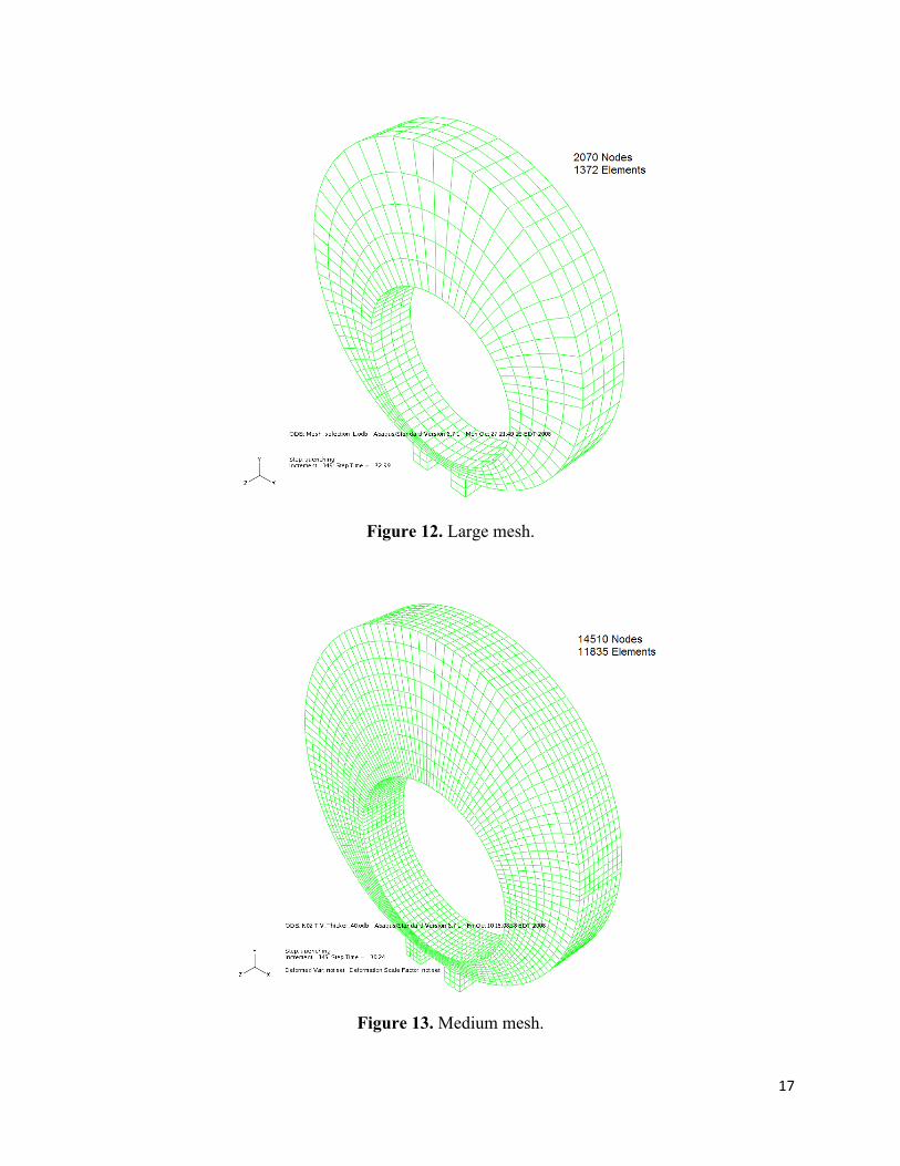
A geometry based on Figure 116 was created and meshed by the ABAQUS pre-processor. The three surface mesh densities shown in Figures 12 to 14 were assessed. In each case, the response of a special node was tracked. This node is most sensitive to mesh refinement since it is located in the thickest section of the part. Only the heat transfer module of the software was used in assessing the effect of mesh density since data is not yet ready for the stress module. Figure 15 shows the time-temperature profile at the selected node during quenching obtained by simulations with the three different mesh densities. Figure 15 shows that the effect of mesh density (within the range tested) on the calculated cooling rate is not significant. The cooling rates of the large and medium mesh are almost identical. However, computational time increases with increasing mesh density. Figure 16 shows the effect of mesh density on computational time for a typical heat transfer simulation. Considering the accuracy of the results and computer time, the medium mesh size was chosen for the analysis. Using the medium mesh, the final meshed geometry contains 11,835 hexahedral elements and 14,510 nodes.

Figure 11. Geometry of the cast component.

6 Courtesy of Montupet S.A., 60180 Nogent Sur Oise, France.

17

Figure 12. Large mesh.

Figure 13. Medium mesh.

18

Figure 14. Small mesh.

Figure 15. Cooling curves at the selected point obtained by simulation with different mesh densities.

19

Figure 16. Computational time for the different mesh densities.

Heat Transfer Simulations

The following sequence was used to model the heat treatment of the part: Furnace-heating to 538°C, followed by a dwell in room temperature air for 6 seconds, followed by immersion into the quench tank with a velocity of 40 mm/s, followed by quenching in water to room temperature. The initial conditions used for the thermal module included the temperature of the part before heat-treating (room temperature in this case), and the mode of heat treatment. The boundary conditions used to represent each of the steps of the heat treatment process were as follows:

− For the furnace-heating step: A convective boundary condition was used at the surface of the part by providing the measured heat transfer coefficient for heating the part in the furnace up to the homogenization temperature of 538°C (1000°F).

− For the dwell step: A convective boundary condition was used at the surface of the part by providing the air heat transfer coefficient (200 W/m2). The ambient temperature was room temperature.

− For the immersion step: The direction and velocity of immersing the part into the quench tank were defined. This step is important in order to capture the temperature gradient along the immersion length of the part. In this demonstration, the part was immersed along (1) its length and (2) its thickness with a velocity of 40 mm/s, and the process time for this step was 3.05 seconds for the vertical quenching and 0.4375 seconds for the horizontal quenching.

9120

1151445

Large Medium Small

=me(S)

20

− For the quenching step: A convective boundary condition at the surface of the part was used by providing the measured heat transfer coefficient for quenching the part in water from the homogenization temperature down to room temperature.

Two heat transfer simulations were performed on the part manufactured as per Sub-Task 2.1 using the ABAQUS model. In the first simulation, the part was quenched vertically into the water tank. In the second simulation, the part was quenched horizontally into the water tank. See Figure 17.

Figure 17. Schematic representation of the directions in which the parts were quenched.

Vertical Immersion – In this simulation, the time for complete immersion is 3.05 s and this time span resulted in a maximum temperature difference of 135.0° C between the bottom surface of the part (the surface that contacted the water first) and the top surface of the part (the surface that contacted the water last). The resulting temperature distribution is shown in Figure 18.

Horizontal Immersion – In this simulation, the time for complete immersion is 0.4375 s and this time span resulted in a maximum temperature difference of 61.3°C between the bottom surface of the part and the top surface of the part. This is a more uniform temperature distribution, compared to the other quenching direction, but causes more temperature difference between the left side of the part (the side that contacted the water first) and right side of the part (the side that contacted the water last). The resulting temperature distribution is shown in Figure 19.

21

Figure 18. Model predicted temperature distribution for vertical quenching.

Figure 19. Model predicted temperature distribution for horizontal quenching.

22

Thermal Stress Analysis

This module uses mainly the time-temperature history of the part, which is generated by the thermal module in order to calculate the residual stresses. For initial condition, the stress at all the nodes was set to zero. If a known initial stress state existed, the appropriate values could be used. Nodal constraints are required in order to prevent rigid body displacement and rotation. This requirement applies to all the process steps, and is defined only once in the model input file. Referring to the 3-D geometry in Figure 19, three nodes at the center of the top face were constrained from moving. For the time being, the necessary high temperature tensile properties are obtained from the open literature [6]. Work is on-going to measure these properties by means of a modified Instron universal testing machine. Results of the quenching-induced distortion and residual stresses are shown in Figure 20. For better visualization, the distortion results are magnified by 100 times.

Figure 20. Model-predicted distortion and residual stresses in MPa induced by vertical quenching in room temperature water.

23

Task 3: Verify the Model Predictions

The model predictions are verified by comparing them to measurements of corresponding parameters for parts made using processing conditions similar to those used in the simulation. The capabilities of the model are demonstrated using the test part7 shown in Figure 21. The parts were heat-treated at WPI. In order to eliminate prior residual stresses in the parts, they were annealed/solutionized at 538°C (1000°F) for 12 hours. In the simulation, it is assumed that this period has elapsed and therefore a stress-free condition represents the initial state of the part. After homogenization, the ring is quenched in water that is maintained at room temperature. Several repetitions were made for both vertical quenching and horizontal quenching.

Figure 21. The cast part.

Measurement of Dimensional Changes and Distortion

A Starrett coordinate measuring machine (CMM) was used to measure the dimensional changes and distortion caused by the heat treatment process. Sufficient measurements will be made in order to obtain accurate representation of the part before and after heat treatment. In order to characterize the amount of distortion in the parts after heat treatment, a fixture was made to hold

7 Courtesy of Montupet S.A., 60180 Nogent Sur Oise, France.

24

the parts at the same location in the CMM, as shown in Figure 22. The fixture was made out of an aluminum block with pins that fit the holes in the part to hold it in a vertical position with its thinnest section pointing up. The middle circular hole of the part was measured before and after heat treatment at locations around the periphery in 10° increments, starting from the thickest section, as shown in red in Figures 22. The x-y data from the CMM measurement was converted into a plot of change in angular radius, as shown in Figures 23(a). The model predictions are shown in Figure 23(b). The curves have a similar shape, but there is significant difference between the model-predicted and the measured values. It is believed that better agreement between the model-predicted and the measured values will be achieved when accurate elevated temperature mechanical properties of the material are made available to the model (i.e., when Sub-Task 1.2 is completed).

Figure 22. The cast part.

25

(a)

(b)

Figure 23: Change in the radius of the inner hole of the solutionized part after vertical quenching in water. (a) Measured, and (b) model-predicted.

‐0.3

‐0.25

‐0.2

‐0.15

‐0.1

‐0.05

0

0.05

0.1

0.15

0 50 100 150 200 250 300 350

Chan

geinra

dius(m

m)

Angle(Degrees)

CMM

‐0.04

‐0.03

‐0.02

‐0.01

0

0.01

0.02

0.03

0 50 100 150 200 250 300 350

Chan

geinra

dius(m

m)

Angle(Degrees)

Model

26

Measurement of Residual Stresses

The standard x-ray diffraction method for measuring residual stresses in metallic components was used. In this method, line shifts due to a uniform strain in the component are measured and then the stresses in the component are determined by a calculation involving the elastic constants of the material. Figure 24 is a schematic representation of a surface under a plain stress condition. By knowing the strain free inter planar spacing d and do, the modulus of elasticity in a specific crystal direction, E, and Poisson’s ratio in that crystal direction, ν, the two components of the biaxial principle stress can be obtained from Eq (3). [7-9]

(3)

Measurements were made in an x-ray diffractometer equipped with a stress analysis module8. The residual stresses were measured at the inner face of the hole in the thinnest section since this location is expected to have the highest magnitude of residual stress. This desired geometry needs to be analyzed at the inside round surface where the maximum residual stresses is located. This gives major restrictions in the X-ray beam paths, as shown in Figure 25. The upper part of the ring will block some of the X-ray beam diffraction angles. Similarly, due to restrictions of geometry, bi-axial stress analysis is also difficult. Therefore, the uni-axial residual stresses analysis is applied, which is the standard method for measuring big sample. Some angles blocked by upper body are shifted, so that received reasonable signal [10]. Figure 26 shows the peak (~157°) and angular range that are used for residual stress analysis.

Figure 27 shows a comparison between the measured and model-predicted magnitude of residual stress in the part. It is clear that there is very good agreement between the measured and the model-predicted residual stresses and that quenching the part vertically creates more residual stresses than quenching it horizontally.

8 Model X’Pert Pro diffractometer manufactured by PANalytical, Inc., Natick, MA, USA.

27

Figure 24: A schematic representation of a surface under plain stress [4].

Figure 25. Diffractometer and location on the part where residual stresses were measured.

Figure 26. Diffraction pattern showing the angular range selected.

28

Figure 27. Residual stresses in the solutionized, water-quenched part. (a) Vertically quenched, and (b) horizontally quenched.

References

1. D. Emadi et al., Optimal Heat Treatment of A356.2 Alloy, Light Metals, (The Minerals, Metals & Materials Society, 2003), 983.

2. D.J. Bammann, M.L. Chiesa, and G.C. Johnson, “Modeling Large Deformation and Failure in Manufacturing Processes,” Proceedings of the Nineteenth International Congress on Theoretical and Applied Mechanics, 1996, 359-376.

3. V. Warke et al., “Modeling the Heat Treatment of Powder Metallurgy Steels and Particulate Materials,” International Conference On Powder Metallurgy and Particulate Materials, 2004, 39-53.

4. M. Maniruzzaman et al., “CHTE Quench Probe System – A NEW Quenchant Characterization System,” Proceedings of the Fifth International Conference on Frontiers of Design and Manufacturing (ICFDM 2002), 1 (2002), 619-625.

5. C.A. Muojekwu, I.V. Samarasekera and J.K. Brimacombe, “Casting-chill Interface Heat Transfer during Solidification of an Aluminum Alloy,” Metall. Mater. Trans, 26 (B), (1995), 361-382.

6. C.M. Estey et al., “Constitutive Behavior of A356 during the Quenching Operation”, Materials Science and Engineering, 383 (A), (2004), 245-251.

7. P.S. Prevey, “A Method of Determining Elastic Constants in Selected Crystallographic Direction for X-Ray Diffraction Residual Stress Measurement,” Advances in X-Ray Analysis, 20 (1977), 345-354.

8. B.D. Cullity and S.R. Stock, “Elements of X-Ray Diffraction,” 3rd edition, Princeton Hall Publications, 2004, 435-468.

9. “Residual Stress Measurement by X-Ray Diffraction,” SAE Standard, J784a, August 1971.

10. V. Guley, “Residual Stress and Retained Austenite X-Ray Diffraction Measurements on Ball Bearings” (Job report No. D030914J, PANalytical Co.), 2003.

96

88.6

92.9492.16

UnitsinMPa

Measured Predicted

(a) (b)