Evaluation of handling of trucks Internship at Scania 04-05-2015 - 31-08-2015 Wilfred Scholten s1010964 Scania CV AB Department RTCD S¨ odert¨ alje, Sweden Supervisor Jolle IJkema University of Twente Faculty of engineering technology Section Applied Mechanics Supervisor Andr´ e de Boer
Transcript
Evaluation of handling oftrucks
Internship at Scania
04-05-2015 - 31-08-2015
Wilfred Scholtens1010964
Scania CV ABDepartment RTCDSodertalje, SwedenSupervisor Jolle IJkema
University of TwenteFaculty of engineering technologySection Applied MechanicsSupervisor Andre de Boer
1. Preface
This report is written during my internship at Scania in Sweden. This internship took place withinthe department RTCD, responsible for testing of trucks on handling, ride & vibration comfort, steeringand mobility. During these four months, I was part of the team and got insight in the work done bythis department. My main assignments considered updating the Matlab scripts used to analyze testdata. However, I also got the possibility to see the work of my colleagues and join a number of tests. Iwould like to thank my colleagues at RTCD. I felt really welcome and was treated as part of the team.Furthermore I would like to thank my supervisor, Jolle, for offering me this opportunity and for being agood host at work but outside the office hours as well.
II
2. Abstract
This internship is done at Scania, within the department responsible for testing of trucks regarding dy-namic aspects. The main assignments during this internship consisted of updating several Matlab basedtools, used to evaluate test data.
Scania uses a number of handling tests in order to judge the handling behavior of truck objectively.During these tests the vehicle is driven at 70km/h and a certain steering movement varied for each testis made. The outcome of these tests is a set of metrics which describe the handling behavior.
The already in use Matlab tool used to evaluate the test data has been revised on several aspects. Testdata from the random test, at which the vehicle is steered to the left and right at an increasing frequency,can now be used to approximate the results of the weave test, were the same is done but at a lower andconstant frequency. Cab and axle roll gradients are calculated in a way less sensitive to influences of aninclined test track or side winds. The asymmetry of some metrics has been studied. Furthermore somepractical changes have been made. This includes the establishment of a database and further automati-sation of storing and presenting the results.
A new script is made to analyze the steering wheel return test. In this test the steering wheel is releasedfrom a large angle while driving at slow speed. The outcomes of the test are the steering wheel anglevelocity and the final steering wheel angle. The new script investigates automatically the suitability ofthe test data as there is a large number of faulty measurements. The new script also provides the optionto compare the results with other tests.
At the end the determination of the ratio from steering wheel to steered front wheel is discussed briefly.This ratio is tested on eleven trucks, the results are used by the ESP system to quickly calculate the yawvelocity. The ESP system will brake certain wheels if the yaw velocity is considered to be to high.
Scania is a manufacturer of trucks and buses and part of the Volkswagen group. Besides complete ve-hicles, Scania sells its engines to serve in many types of machinery and vessels. Nowadays services arebecoming a more important product of the company as well. Scania is a global company with efficientfactories all over the world. The company uses principles as lean manufacturing and house of quality,to eliminate waste, meet costumer demands and keep improving its processes. These principles are notonly used in production but throughout the whole company.
Scania trucks are based on a modular system in which many components are interchangeable. Thisenables the company to produce a large variety of trucks easily in order to meet specific customer de-mands. The number of different parts is kept surprisingly low, which improves efficiency in productionand logistics. Furthermore new designs or technologies can be implemented quickly as a result of themodular system.
Although production is scattered around Europe and the rest of the world, almost all research and de-velopment work is done in Sodertalje, Sweden. This internship took place in Sodertalje at the ScaniaTekniskt Centrum. Here, employees have access to many facilities. Examples are engine test cells, rigstesting the fatigue life of different components and the test track.
RTC is the department responsible for the vehicle dynamics and chassis design. It is part of a largerdepartment developing trucks. This internship took place at the group RTCD, which is one of thesubdivisions of RTC. Directly cited from the homepage [1], RTCD is responsible for complete vehicletesting for Scania truck product-development in handling, ride & vibration comfort, steering and mobility.Other groups within RTC are responsible for [1]:
� Steering design
� Basic chassis development design
� Dynamics and strength analysis
� Gear shift, cab tilt and trailer connection design
� Brake performance
1.1 Department RTCD
The group consist of about 20 employees, these are not only engineers but mechanics as well. Most ofthem have truck driving licenses and can be found on the local test track regularly. As mentioned earlierthe focus of the group can roughly be separated in four fields of interests [1]:
� Handling: keeping and improving the vehicle handling which is characterized by on-course stabilityand quick vehicle response.
� Ride- & vibration comfort: Improving the vehicle ride- and vibration comfort by lowering the cabvibration level.
� Steering: Developing precise and responsive steering systems.
1
� Mobility: Increasing traction capability to allow for greater mobility on all-terrains.
The vehicle dynamic properties related to these four subjects are tested both objective and subjective.It is hard to judge the driving behavior on basis of the complex related objective measures only. That iswhere the experienced drivers come in. Driving properties are rated on a 1 to 10 scale by drivers opinion,the goal is to relate all objective measurements to such a scale as well.
My tasks within this department were mainly to improve Matlab scripts already in use to analyse testdata. These scripts mainly refered to the steering design part of the department. Furthermore some testdata has been analyzed and an internal report has been written. Besides working on these tasks I gotthe possibility to join on several tests and got an overall view of what kind of work was being done bythis department and Scania in general. The main assignments will be elaborated in chapter 3 to chapter5 after an introduction to the subject of vehicle dynamics in chapter 2.
2
2. Vehicle dynamics
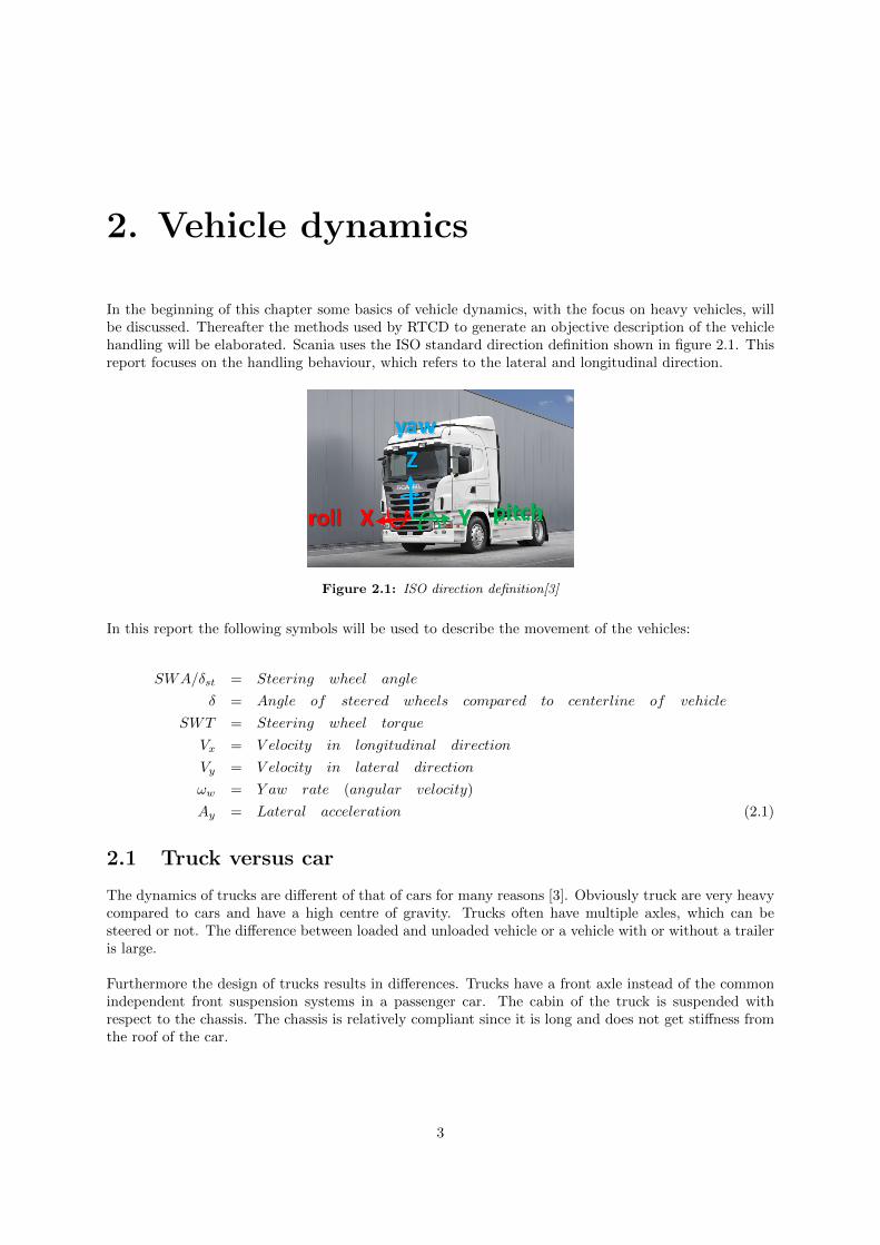
In the beginning of this chapter some basics of vehicle dynamics, with the focus on heavy vehicles, willbe discussed. Thereafter the methods used by RTCD to generate an objective description of the vehiclehandling will be elaborated. Scania uses the ISO standard direction definition shown in figure 2.1. Thisreport focuses on the handling behaviour, which refers to the lateral and longitudinal direction.
Figure 2.1: ISO direction definition[3]
In this report the following symbols will be used to describe the movement of the vehicles:
SWA/δst = Steering wheel angle
δ = Angle of steered wheels compared to centerline of vehicle
SWT = Steering wheel torque
Vx = V elocity in longitudinal direction
Vy = V elocity in lateral direction
ωw = Y aw rate (angular velocity)
Ay = Lateral acceleration (2.1)
2.1 Truck versus car
The dynamics of trucks are different of that of cars for many reasons [3]. Obviously truck are very heavycompared to cars and have a high centre of gravity. Trucks often have multiple axles, which can besteered or not. The difference between loaded and unloaded vehicle or a vehicle with or without a traileris large.
Furthermore the design of trucks results in differences. Trucks have a front axle instead of the commonindependent front suspension systems in a passenger car. The cabin of the truck is suspended withrespect to the chassis. The chassis is relatively compliant since it is long and does not get stiffness fromthe roof of the car.
3
2.2 Handling diagram
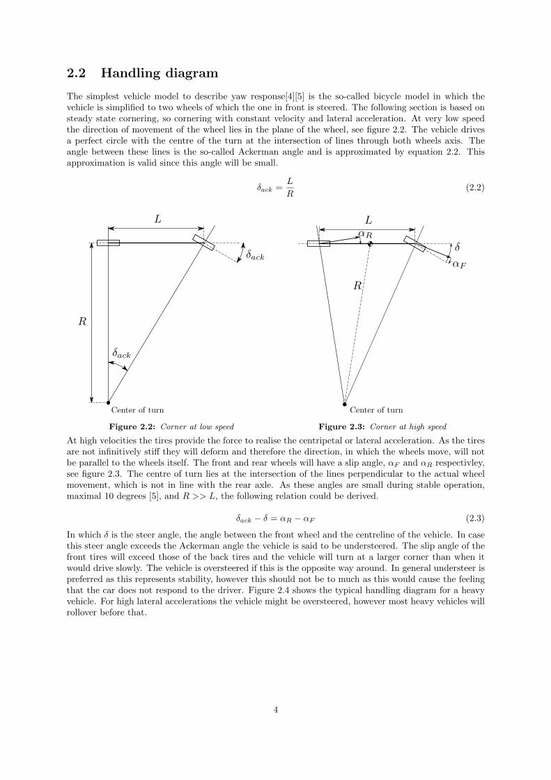
The simplest vehicle model to describe yaw response[4][5] is the so-called bicycle model in which thevehicle is simplified to two wheels of which the one in front is steered. The following section is based onsteady state cornering, so cornering with constant velocity and lateral acceleration. At very low speedthe direction of movement of the wheel lies in the plane of the wheel, see figure 2.2. The vehicle drivesa perfect circle with the centre of the turn at the intersection of lines through both wheels axis. Theangle between these lines is the so-called Ackerman angle and is approximated by equation 2.2. Thisapproximation is valid since this angle will be small.
δack =L
R(2.2)
Figure 2.2: Corner at low speed Figure 2.3: Corner at high speed
At high velocities the tires provide the force to realise the centripetal or lateral acceleration. As the tiresare not infinitively stiff they will deform and therefore the direction, in which the wheels move, will notbe parallel to the wheels itself. The front and rear wheels will have a slip angle, αF and αR respectivley,see figure 2.3. The centre of turn lies at the intersection of the lines perpendicular to the actual wheelmovement, which is not in line with the rear axle. As these angles are small during stable operation,maximal 10 degrees [5], and R >> L, the following relation could be derived.
δack − δ = αR − αF (2.3)
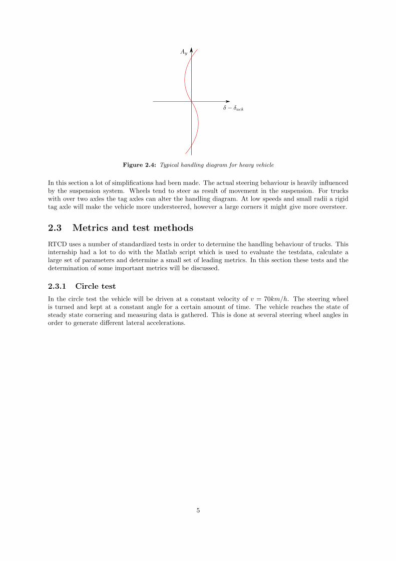
In which δ is the steer angle, the angle between the front wheel and the centreline of the vehicle. In casethis steer angle exceeds the Ackerman angle the vehicle is said to be understeered. The slip angle of thefront tires will exceed those of the back tires and the vehicle will turn at a larger corner than when itwould drive slowly. The vehicle is oversteered if this is the opposite way around. In general understeer ispreferred as this represents stability, however this should not be to much as this would cause the feelingthat the car does not respond to the driver. Figure 2.4 shows the typical handling diagram for a heavyvehicle. For high lateral accelerations the vehicle might be oversteered, however most heavy vehicles willrollover before that.
4
Figure 2.4: Typical handling diagram for heavy vehicle
In this section a lot of simplifications had been made. The actual steering behaviour is heavily influencedby the suspension system. Wheels tend to steer as result of movement in the suspension. For truckswith over two axles the tag axles can alter the handling diagram. At low speeds and small radii a rigidtag axle will make the vehicle more understeered, however a large corners it might give more oversteer.
2.3 Metrics and test methods
RTCD uses a number of standardized tests in order to determine the handling behaviour of trucks. Thisinternship had a lot to do with the Matlab script which is used to evaluate the testdata, calculate alarge set of parameters and determine a small set of leading metrics. In this section these tests and thedetermination of some important metrics will be discussed.
2.3.1 Circle test
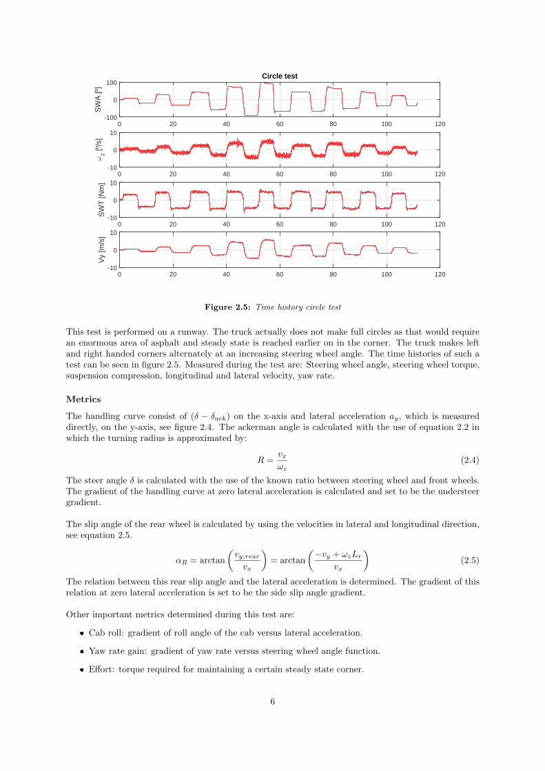
In the circle test the vehicle will be driven at a constant velocity of v = 70km/h. The steering wheelis turned and kept at a constant angle for a certain amount of time. The vehicle reaches the state ofsteady state cornering and measuring data is gathered. This is done at several steering wheel angles inorder to generate different lateral accelerations.
5
0 20 40 60 80 100 120
SW
A [º
]
-100
0
100Circle test
0 20 40 60 80 100 120
ωz [º
/s]
-10
0
10
0 20 40 60 80 100 120
SW
T [N
m]
-10
0
10
0 20 40 60 80 100 120
Vy
[m/s
]
-10
0
10
Figure 2.5: Time history circle test
This test is performed on a runway. The truck actually does not make full circles as that would requirean enormous area of asphalt and steady state is reached earlier on in the corner. The truck makes leftand right handed corners alternately at an increasing steering wheel angle. The time histories of such atest can be seen in figure 2.5. Measured during the test are: Steering wheel angle, steering wheel torque,suspension compression, longitudinal and lateral velocity, yaw rate.
Metrics
The handling curve consist of (δ − δack) on the x-axis and lateral acceleration ay, which is measureddirectly, on the y-axis, see figure 2.4. The ackerman angle is calculated with the use of equation 2.2 inwhich the turning radius is approximated by:
R =vxωz
(2.4)
The steer angle δ is calculated with the use of the known ratio between steering wheel and front wheels.The gradient of the handling curve at zero lateral acceleration is calculated and set to be the understeergradient.
The slip angle of the rear wheel is calculated by using the velocities in lateral and longitudinal direction,see equation 2.5.
αR = arctan
(vy,rearvx
)= arctan
(−vy + ωzLr
vx
)(2.5)
The relation between this rear slip angle and the lateral acceleration is determined. The gradient of thisrelation at zero lateral acceleration is set to be the side slip angle gradient.
Other important metrics determined during this test are:
� Cab roll: gradient of roll angle of the cab versus lateral acceleration.
� Yaw rate gain: gradient of yaw rate versus steering wheel angle function.
� Effort: torque required for maintaining a certain steady state corner.
6
2.3.2 Random test
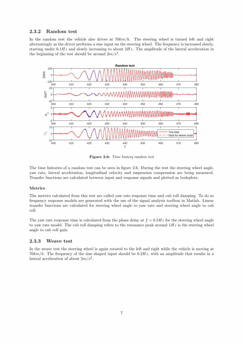
In the random test the vehicle also drives at 70km/h. The steering wheel is turned left and rightalternatingly as the driver performs a sine input on the steering wheel. The frequency is increased slowly,starting under 0.1Hz and slowly increasing to about 2Hz. The amplitude of the lateral acceleration inthe beginning of the test should be around 2m/s2.
400 410 420 430 440 450 460 470 480
SW
A
-100
0
100Random test
400 410 420 430 440 450 460 470 480
SW
T
-20
0
20
400 410 420 430 440 450 460 470 480
Ay
-5
0
5
T400 410 420 430 440 450 460 470 480
ωz
-10
0
10
Test dataInput for weave script
Figure 2.6: Time history random test
The time histories of a random test can be seen in figure 2.6. During the test the steering wheel angle,yaw rate, lateral acceleration, longitudinal velocity and suspension compression are being measured.Transfer functions are calculated between input and response signals and plotted as bodeplots.
Metrics
The metrics calculated from this test are called yaw rate response time and cab roll damping. To do sofrequency response models are generated with the use of the signal analysis toolbox in Matlab. Lineartransfer functions are calculated for steering wheel angle to yaw rate and steering wheel angle to cabroll.
The yaw rate response time is calculated from the phase delay at f = 0.5Hz for the steering wheel angleto yaw rate model. The cab roll damping refers to the resonance peak around 1Hz is the steering wheelangle to cab roll gain.
2.3.3 Weave test
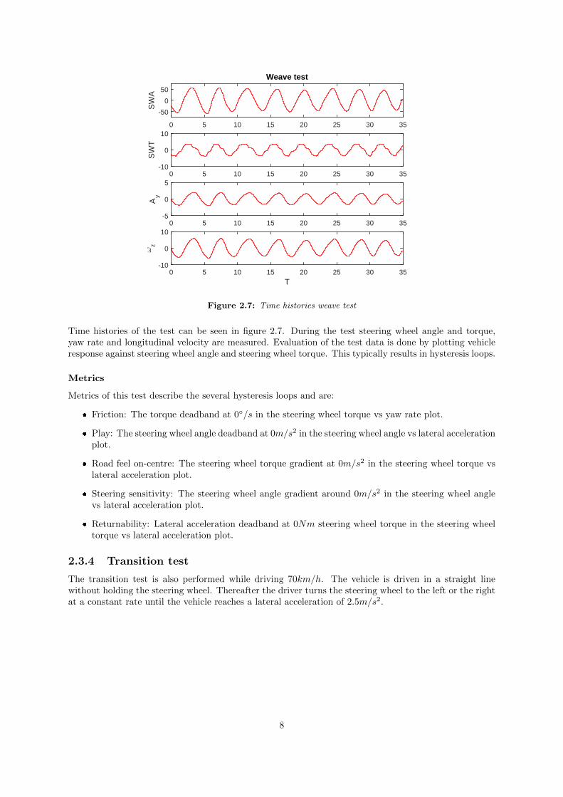
In the weave test the steering wheel is again rotated to the left and right while the vehicle is moving at70km/h. The frequency of the sine shaped input should be 0.2Hz, with an amplitude that results in alateral acceleration of about 2m/s2.
7
0 5 10 15 20 25 30 35
SW
A
-50
0
50
Weave test
0 5 10 15 20 25 30 35
SW
T
-10
0
10
0 5 10 15 20 25 30 35
Ay
-5
0
5
T0 5 10 15 20 25 30 35
ωz
-10
0
10
Figure 2.7: Time histories weave test
Time histories of the test can be seen in figure 2.7. During the test steering wheel angle and torque,yaw rate and longitudinal velocity are measured. Evaluation of the test data is done by plotting vehicleresponse against steering wheel angle and steering wheel torque. This typically results in hysteresis loops.
Metrics
Metrics of this test describe the several hysteresis loops and are:
� Friction: The torque deadband at 0◦/s in the steering wheel torque vs yaw rate plot.
� Play: The steering wheel angle deadband at 0m/s2 in the steering wheel angle vs lateral accelerationplot.
� Road feel on-centre: The steering wheel torque gradient at 0m/s2 in the steering wheel torque vslateral acceleration plot.
� Steering sensitivity: The steering wheel angle gradient around 0m/s2 in the steering wheel anglevs lateral acceleration plot.
� Returnability: Lateral acceleration deadband at 0Nm steering wheel torque in the steering wheeltorque vs lateral acceleration plot.
2.3.4 Transition test
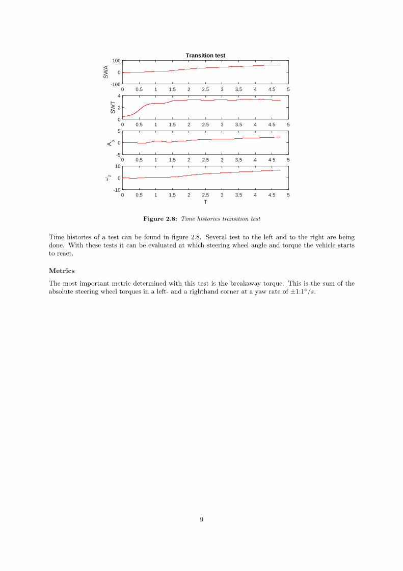
The transition test is also performed while driving 70km/h. The vehicle is driven in a straight linewithout holding the steering wheel. Thereafter the driver turns the steering wheel to the left or the rightat a constant rate until the vehicle reaches a lateral acceleration of 2.5m/s2.
8
0 0.5 1 1.5 2 2.5 3 3.5 4 4.5 5
SW
T0
2
4
0 0.5 1 1.5 2 2.5 3 3.5 4 4.5 5
Ay
-5
0
5
T0 0.5 1 1.5 2 2.5 3 3.5 4 4.5 5
ωz
-10
0
10
0 0.5 1 1.5 2 2.5 3 3.5 4 4.5 5
SW
A
-100
0
100Transition test
Figure 2.8: Time histories transition test
Time histories of a test can be found in figure 2.8. Several test to the left and to the right are beingdone. With these tests it can be evaluated at which steering wheel angle and torque the vehicle startsto react.
Metrics
The most important metric determined with this test is the breakaway torque. This is the sum of theabsolute steering wheel torques in a left- and a righthand corner at a yaw rate of ±1.1◦/s.
9
3. Update of handling script
At RTCD a Matlab script is used to analyse testdata from the handling tests discussed in the previouschapter. My tasks was to update this script on several points and make the script even more functional.The calculation and simulation group within RTC as well as a group working on buses want to use thescript as well. Some adjustments needed to be made in order to run their simulation data generatedwith multibody dynamics program Adams.
In this chapter the major changes regarding the calculations done by the script will be discussed. At theend a list of more practical addjustments is presented.
3.1 Roll gradients
3.1.1 Assignment
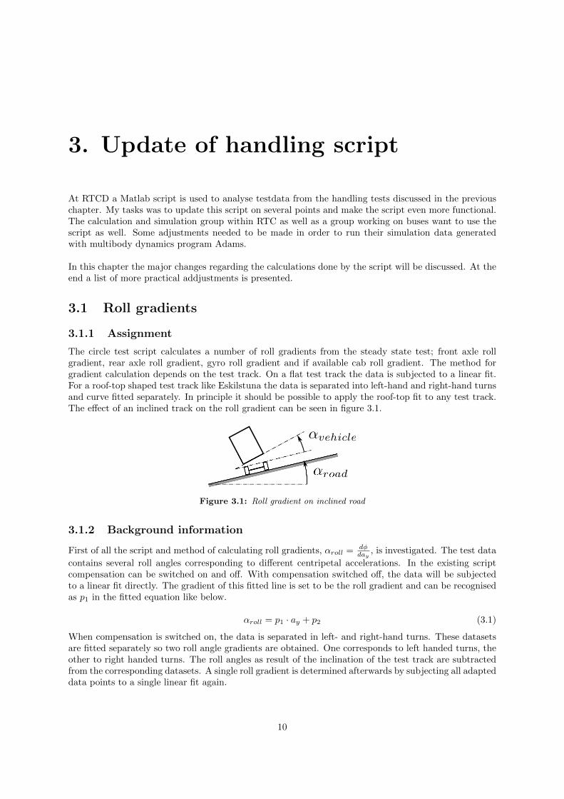
The circle test script calculates a number of roll gradients from the steady state test; front axle rollgradient, rear axle roll gradient, gyro roll gradient and if available cab roll gradient. The method forgradient calculation depends on the test track. On a flat test track the data is subjected to a linear fit.For a roof-top shaped test track like Eskilstuna the data is separated into left-hand and right-hand turnsand curve fitted separately. In principle it should be possible to apply the roof-top fit to any test track.The effect of an inclined track on the roll gradient can be seen in figure 3.1.
Figure 3.1: Roll gradient on inclined road
3.1.2 Background information
First of all the script and method of calculating roll gradients, αroll = dφday
, is investigated. The test data
contains several roll angles corresponding to different centripetal accelerations. In the existing scriptcompensation can be switched on and off. With compensation switched off, the data will be subjectedto a linear fit directly. The gradient of this fitted line is set to be the roll gradient and can be recognisedas p1 in the fitted equation like below.
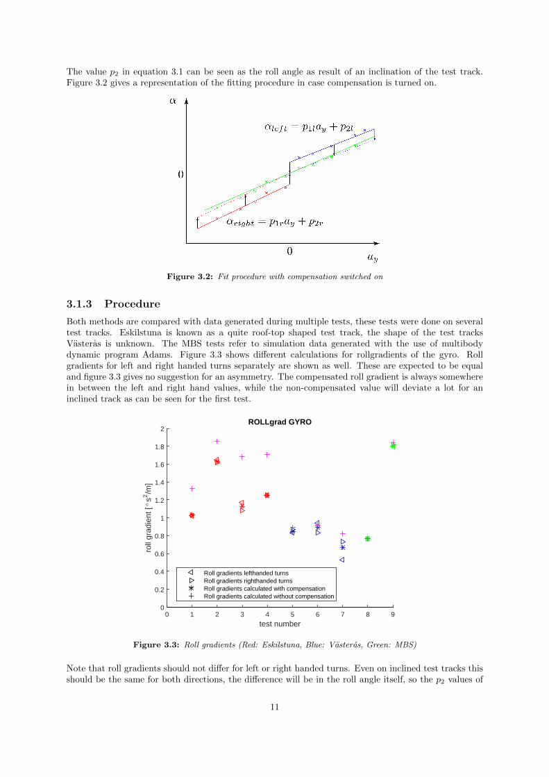
αroll = p1 · ay + p2 (3.1)
When compensation is switched on, the data is separated in left- and right-hand turns. These datasetsare fitted separately so two roll angle gradients are obtained. One corresponds to left handed turns, theother to right handed turns. The roll angles as result of the inclination of the test track are subtractedfrom the corresponding datasets. A single roll gradient is determined afterwards by subjecting all adapteddata points to a single linear fit again.
10
The value p2 in equation 3.1 can be seen as the roll angle as result of an inclination of the test track.Figure 3.2 gives a representation of the fitting procedure in case compensation is turned on.
Figure 3.2: Fit procedure with compensation switched on
3.1.3 Procedure
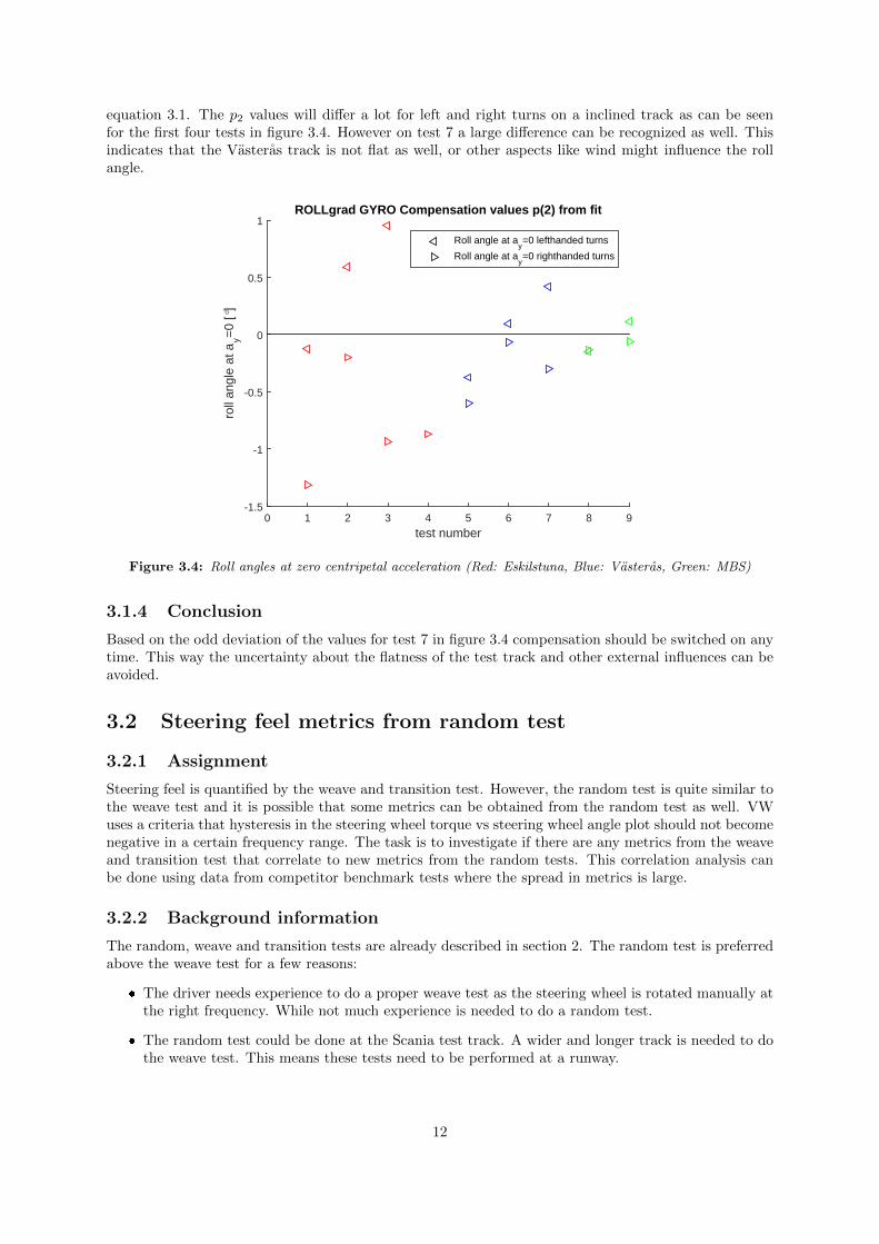
Both methods are compared with data generated during multiple tests, these tests were done on severaltest tracks. Eskilstuna is known as a quite roof-top shaped test track, the shape of the test tracksVasteras is unknown. The MBS tests refer to simulation data generated with the use of multibodydynamic program Adams. Figure 3.3 shows different calculations for rollgradients of the gyro. Rollgradients for left and right handed turns separately are shown as well. These are expected to be equaland figure 3.3 gives no suggestion for an asymmetry. The compensated roll gradient is always somewherein between the left and right hand values, while the non-compensated value will deviate a lot for aninclined track as can be seen for the first test.
test number0 1 2 3 4 5 6 7 8 9
roll
grad
ient
[° s
2/m
]
0
0.2
0.4
0.6
0.8
1
1.2
1.4
1.6
1.8
2ROLLgrad GYRO
Roll gradients lefthanded turnsRoll gradients righthanded turnsRoll gradients calculated with compensationRoll gradients calculated without compensation
Figure 3.3: Roll gradients (Red: Eskilstuna, Blue: Vasteras, Green: MBS)
Note that roll gradients should not differ for left or right handed turns. Even on inclined test tracks thisshould be the same for both directions, the difference will be in the roll angle itself, so the p2 values of
11
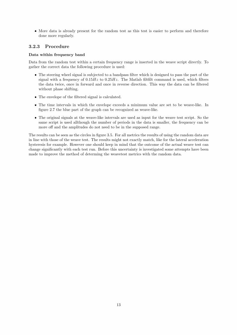
equation 3.1. The p2 values will differ a lot for left and right turns on a inclined track as can be seenfor the first four tests in figure 3.4. However on test 7 a large difference can be recognized as well. Thisindicates that the Vasteras track is not flat as well, or other aspects like wind might influence the rollangle.
test number0 1 2 3 4 5 6 7 8 9
roll
angl
e at
ay=
0 [°
]
-1.5
-1
-0.5
0
0.5
1ROLLgrad GYRO Compensation values p(2) from fit
Roll angle at ay=0 lefthanded turns
Roll angle at ay=0 righthanded turns
Figure 3.4: Roll angles at zero centripetal acceleration (Red: Eskilstuna, Blue: Vasteras, Green: MBS)
3.1.4 Conclusion
Based on the odd deviation of the values for test 7 in figure 3.4 compensation should be switched on anytime. This way the uncertainty about the flatness of the test track and other external influences can beavoided.
3.2 Steering feel metrics from random test
3.2.1 Assignment
Steering feel is quantified by the weave and transition test. However, the random test is quite similar tothe weave test and it is possible that some metrics can be obtained from the random test as well. VWuses a criteria that hysteresis in the steering wheel torque vs steering wheel angle plot should not becomenegative in a certain frequency range. The task is to investigate if there are any metrics from the weaveand transition test that correlate to new metrics from the random tests. This correlation analysis canbe done using data from competitor benchmark tests where the spread in metrics is large.
3.2.2 Background information
The random, weave and transition tests are already described in section 2. The random test is preferredabove the weave test for a few reasons:
� The driver needs experience to do a proper weave test as the steering wheel is rotated manually atthe right frequency. While not much experience is needed to do a random test.
� The random test could be done at the Scania test track. A wider and longer track is needed to dothe weave test. This means these tests need to be performed at a runway.
12
� More data is already present for the random test as this test is easier to perform and thereforedone more regularly.
3.2.3 Procedure
Data within frequency band
Data from the random test within a certain frequency range is inserted in the weave script directly. Togather the correct data the following procedure is used:
� The steering wheel signal is subjected to a bandpass filter which is designed to pass the part of thesignal with a frequency of 0.15Hz to 0.25Hz. The Matlab filtfilt command is used, which filtersthe data twice, once in forward and once in reverse direction. This way the data can be filteredwithout phase shifting.
� The envelope of the filtered signal is calculated.
� The time intervals in which the envelope exceeds a minimum value are set to be weave-like. Infigure 2.7 the blue part of the graph can be recognized as weave-like.
� The original signals at the weave-like intervals are used as input for the weave test script. So thesame script is used allthough the number of periods in the data is smaller, the frequency can bemore off and the amplitudes do not need to be in the supposed range.
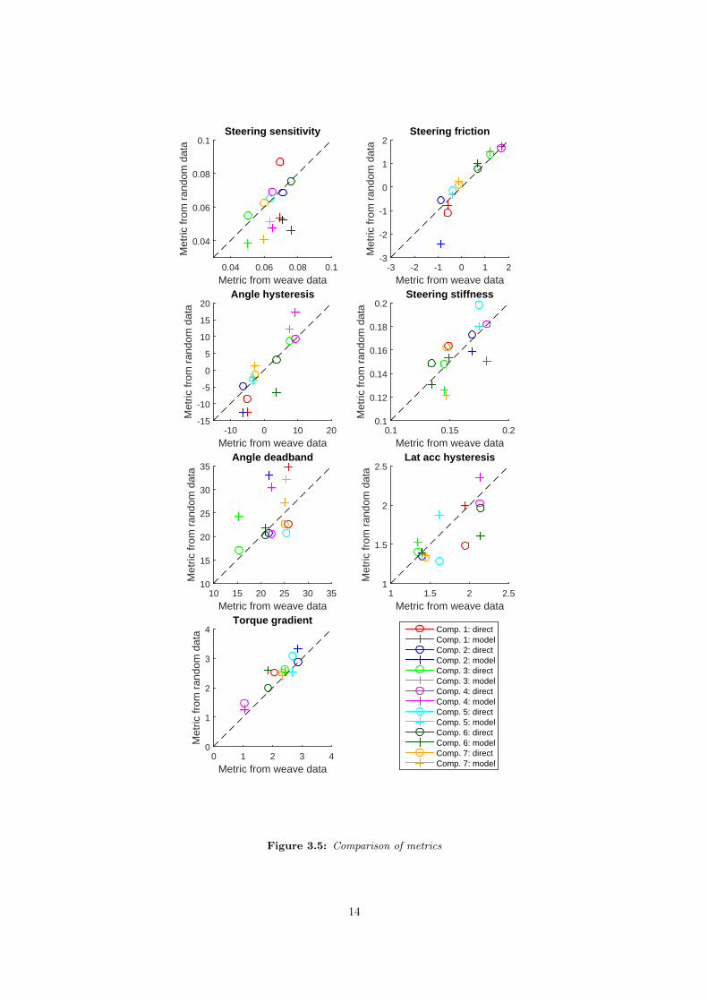
The results can be seen as the circles in figure 3.5. For all metrics the results of using the random data arein line with those of the weave test. The results might not exactly match, like for the lateral accelerationhysteresis for example. However one should keep in mind that the outcome of the actual weave test canchange significantly with each test run. Before this uncertainty is investigated some attempts have beenmade to improve the method of determing the weavetest metrics with the random data.
The area of the hysteresis loops is calculated for several trucks as it was expected to be related to thewidth or height of the loops. Furthermore this area is in theory related to the phase shift of the transferfunction, which might be easier to predict with the data form the random test.
It turned out to be hard to calculate this hysteresis area properly. Difficulties arise since each loop is abit different, also the starting and end point of the loop are variable. The approximated hysteresis areasshowed no clear correlation with the deadbands.
Synthetic signal
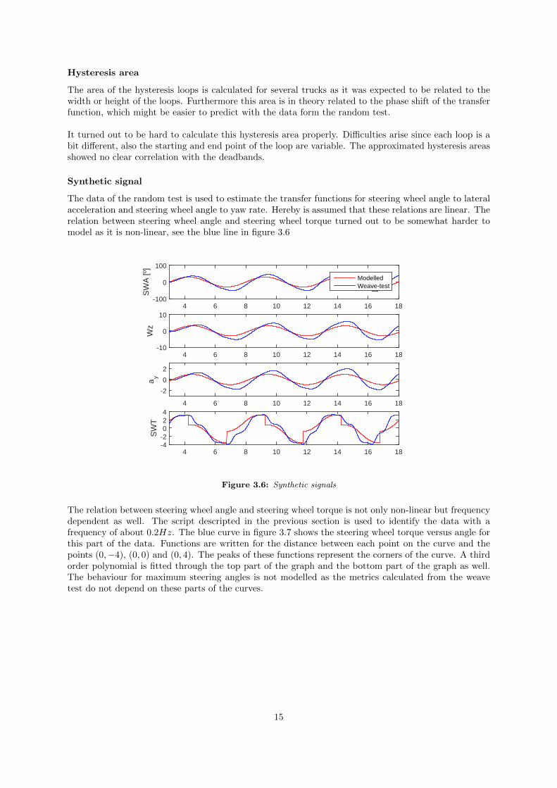
The data of the random test is used to estimate the transfer functions for steering wheel angle to lateralacceleration and steering wheel angle to yaw rate. Hereby is assumed that these relations are linear. Therelation between steering wheel angle and steering wheel torque turned out to be somewhat harder tomodel as it is non-linear, see the blue line in figure 3.6
4 6 8 10 12 14 16 18
SW
A [º
]
-100
0
100
ModelledWeave-test
4 6 8 10 12 14 16 18
Wz
-10
0
10
4 6 8 10 12 14 16 18
ay
-2
0
2
4 6 8 10 12 14 16 18
SW
T
-4-2024
Figure 3.6: Synthetic signals
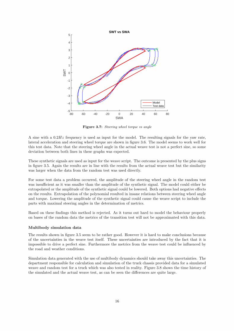
The relation between steering wheel angle and steering wheel torque is not only non-linear but frequencydependent as well. The script descripted in the previous section is used to identify the data with afrequency of about 0.2Hz. The blue curve in figure 3.7 shows the steering wheel torque versus angle forthis part of the data. Functions are written for the distance between each point on the curve and thepoints (0,−4), (0, 0) and (0, 4). The peaks of these functions represent the corners of the curve. A thirdorder polynomial is fitted through the top part of the graph and the bottom part of the graph as well.The behaviour for maximum steering angles is not modelled as the metrics calculated from the weavetest do not depend on these parts of the curves.
15
SWA-80 -60 -40 -20 0 20 40 60 80
SW
T
-5
-4
-3
-2
-1
0
1
2
3
4
5SWT vs SWA
ModelTest data
Figure 3.7: Steering wheel torque vs angle
A sine with a 0.2Hz frequency is used as input for the model. The resulting signals for the yaw rate,lateral acceleration and steering wheel torque are shown in figure 3.6. The model seems to work well forthis test data. Note that the steering wheel angle in the actual weave test is not a perfect sine, so somedeviation between both lines in these graphs was expected.
These synthetic signals are used as input for the weave script. The outcome is presented by the plus signsin figure 3.5. Again the results are in line with the results from the actual weave test but the similaritywas larger when the data from the random test was used directly.
For some test data a problem occurred, the amplitude of the steering wheel angle in the random testwas insufficient as it was smaller than the amplitude of the synthetic signal. The model could either beextrapolated or the amplitude of the synthetic signal could be lowered. Both options had negative effectson the results. Extrapolation of the polynomial resulted in insane relations between steering wheel angleand torque. Lowering the amplitude of the synthetic signal could cause the weave script to include theparts with maximal steering angles in the determination of metrics.
Based on these findings this method is rejected. As it turns out hard to model the behaviour properlyon bases of the random data the metrics of the transition test will not be approximated with this data.
Multibody simulation data
The results shown in figure 3.5 seem to be rather good. However it is hard to make conclusions becauseof the uncertainties in the weave test itself. These uncertainties are introduced by the fact that it isimpossible to drive a perfect sine. Furthermore the metrics from the weave test could be influenced bythe road and weather conditions.
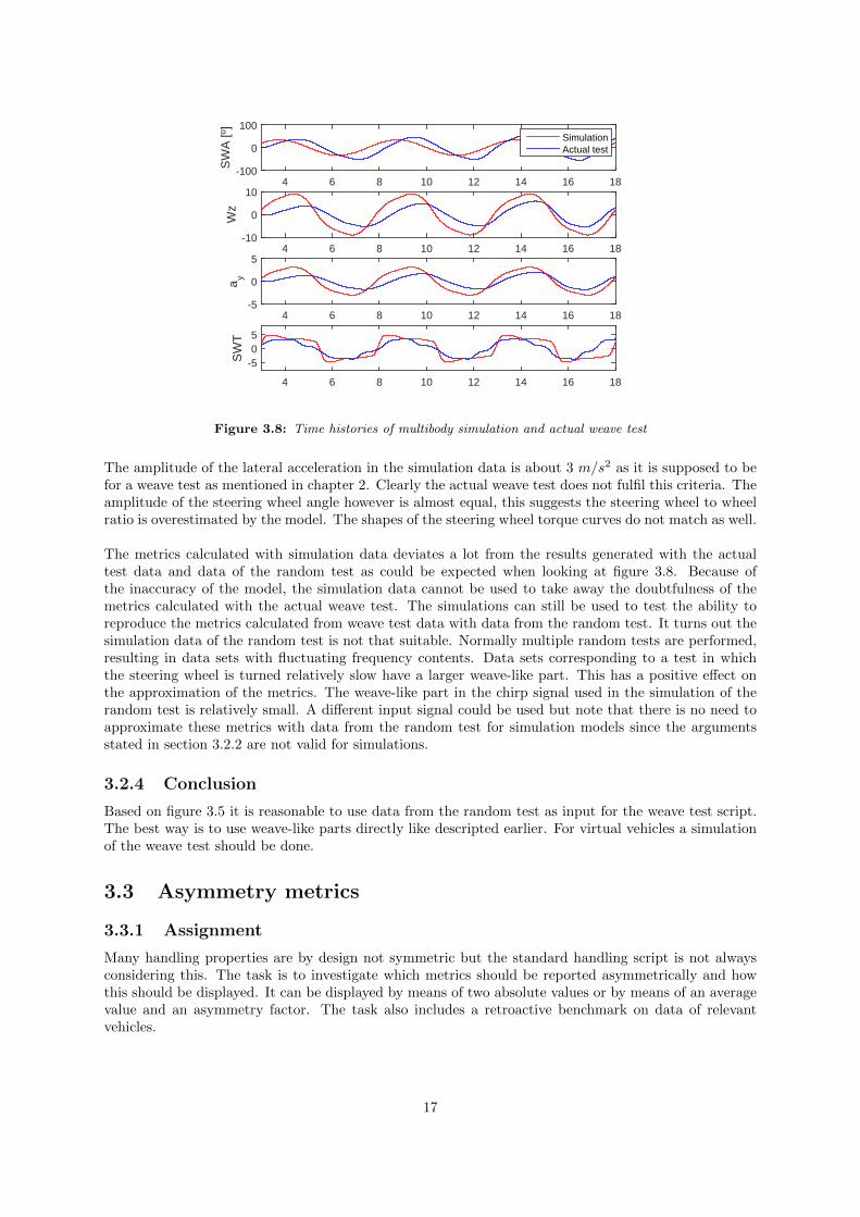
Simulation data generated with the use of multibody dynamics should take away this uncertainties. Thedepartment responsible for calculation and simulation of the truck chassis provided data for a simulatedweave and random test for a truck which was also tested in reality. Figure 3.8 shows the time history ofthe simulated and the actual weave test, as can be seen the differences are quite large.
16
4 6 8 10 12 14 16 18
SW
A [º
]
-100
0
100SimulationActual test
4 6 8 10 12 14 16 18
Wz
-10
0
10
4 6 8 10 12 14 16 18
ay
-5
0
5
4 6 8 10 12 14 16 18
SW
T
-505
Figure 3.8: Time histories of multibody simulation and actual weave test
The amplitude of the lateral acceleration in the simulation data is about 3 m/s2 as it is supposed to befor a weave test as mentioned in chapter 2. Clearly the actual weave test does not fulfil this criteria. Theamplitude of the steering wheel angle however is almost equal, this suggests the steering wheel to wheelratio is overestimated by the model. The shapes of the steering wheel torque curves do not match as well.
The metrics calculated with simulation data deviates a lot from the results generated with the actualtest data and data of the random test as could be expected when looking at figure 3.8. Because ofthe inaccuracy of the model, the simulation data cannot be used to take away the doubtfulness of themetrics calculated with the actual weave test. The simulations can still be used to test the ability toreproduce the metrics calculated from weave test data with data from the random test. It turns out thesimulation data of the random test is not that suitable. Normally multiple random tests are performed,resulting in data sets with fluctuating frequency contents. Data sets corresponding to a test in whichthe steering wheel is turned relatively slow have a larger weave-like part. This has a positive effect onthe approximation of the metrics. The weave-like part in the chirp signal used in the simulation of therandom test is relatively small. A different input signal could be used but note that there is no need toapproximate these metrics with data from the random test for simulation models since the argumentsstated in section 3.2.2 are not valid for simulations.
3.2.4 Conclusion
Based on figure 3.5 it is reasonable to use data from the random test as input for the weave test script.The best way is to use weave-like parts directly like descripted earlier. For virtual vehicles a simulationof the weave test should be done.
3.3 Asymmetry metrics
3.3.1 Assignment
Many handling properties are by design not symmetric but the standard handling script is not alwaysconsidering this. The task is to investigate which metrics should be reported asymmetrically and howthis should be displayed. It can be displayed by means of two absolute values or by means of an averagevalue and an asymmetry factor. The task also includes a retroactive benchmark on data of relevantvehicles.
17
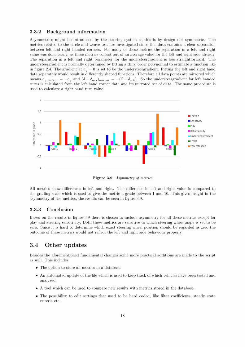
3.3.2 Background information
Asymmetries might be introduced by the steering system as this is by design not symmetric. Themetrics related to the circle and weave test are investigated since this data contains a clear separationbetween left and right handed corners. For many of these metrics the separation in a left and rightvalue was done easily, as these metrics consist out of an average value for the left and right side already.The separation in a left and right parameter for the understeergradient is less straightforward. Theundersteergradient is normally determined by fitting a third order polynomial to estimate a function likein figure 2.4. The gradient at ay = 0 is set to be the understeergradient. Fitting the left and right handdata separately would result in differently shaped functions. Therefore all data points are mirrored whichmeans ay,mirror = −ay and (δ − δack)mirror = −(δ − δack). So the understeergradient for left handedturns is calculated from the left hand corner data and its mirrored set of data. The same procedure isused to calculate a right hand turn value.
Figure 3.9: Asymmetry of metrics
All metrics show differences in left and right. The difference in left and right value is compared tothe grading scale which is used to give the metric a grade between 1 and 10. This gives insight in theasymmetry of the metrics, the results can be seen in figure 3.9.
3.3.3 Conclusion
Based on the results in figure 3.9 there is chosen to include asymmetry for all these metrics except forplay and steering sensitivity. Both these metrics are sensitive to which steering wheel angle is set to bezero. Since it is hard to determine which exact steering wheel position should be regarded as zero theoutcome of these metrics would not reflect the left and right side behaviour properly.
3.4 Other updates
Besides the aforementioned fundamental changes some more practical additions are made to the scriptas well. This includes:
� The option to store all metrics in a database.
� An automated update of the file which is used to keep track of which vehicles have been tested andanalyzed.
� A tool which can be used to compare new results with metrics stored in the database.
� The possibility to edit settings that used to be hard coded, like filter coefficients, steady statecriteria etc.
18
4. Steering wheel return script
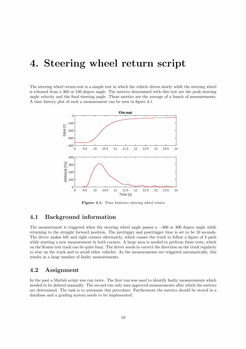
The steering wheel return test is a simple test in which the vehicle drives slowly while the steering wheelis released from a 360 or 540 degree angle. The metrics determined with this test are the peak steeringangle velocity and the final steering angle. These metrics are the average of a bunch of measurements.A time history plot of such a measurement can be seen in figure 4.1.
9 9.5 10 10.5 11 11.5 12 12.5 13 13.5 14
SW
A [º
]
-400
-300
-200
-100
0File.mat
Time [s]9 9.5 10 10.5 11 11.5 12 12.5 13 13.5 14
dSW
A/d
t [º/
s]
0
100
200
300
400
Figure 4.1: Time histories steering wheel return
4.1 Background information
The measurement is triggered when the steering wheel angle passes a −300 or 300 degree angle whilereturning to the straight forward position. The pretrigger and posttrigger time is set to be 10 seconds.The driver makes left and right corners alternately, which causes the truck to follow a figure of 8 pathwhile starting a new measurement in both corners. A large area is needed to perform these tests, whichon the Scania test track can be quite busy. The driver needs to correct the direction on the truck regularlyto stay on the track and to avoid other vehicles. As the measurements are triggered automatically, thisresults in a large number of faulty measurements.
4.2 Assignment
In the past a Matlab script was run twice. The first run was used to identify faulty measurements whichneeded to be deleted manually. The second run only uses approved measurements after which the metricsare determined. The task is to automate this procedure. Furthermore the metrics should be stored in adatabase and a grading system needs to be implemented.
19
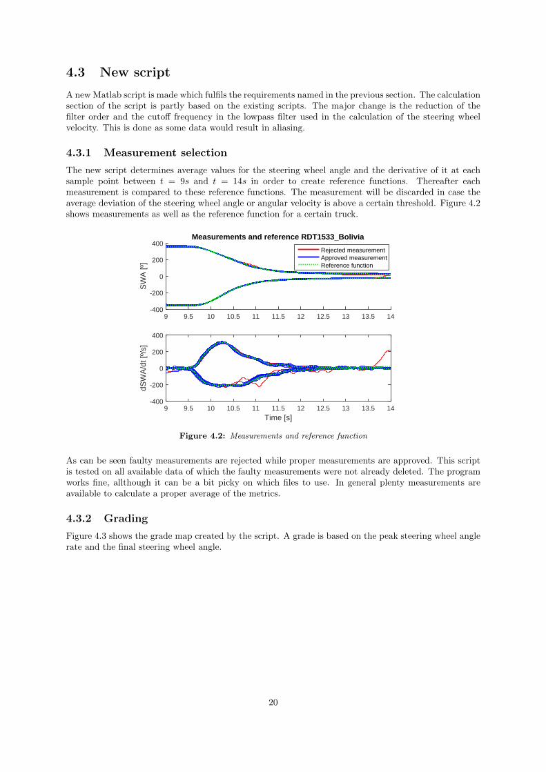
4.3 New script
A new Matlab script is made which fulfils the requirements named in the previous section. The calculationsection of the script is partly based on the existing scripts. The major change is the reduction of thefilter order and the cutoff frequency in the lowpass filter used in the calculation of the steering wheelvelocity. This is done as some data would result in aliasing.
4.3.1 Measurement selection
The new script determines average values for the steering wheel angle and the derivative of it at eachsample point between t = 9s and t = 14s in order to create reference functions. Thereafter eachmeasurement is compared to these reference functions. The measurement will be discarded in case theaverage deviation of the steering wheel angle or angular velocity is above a certain threshold. Figure 4.2shows measurements as well as the reference function for a certain truck.
9 9.5 10 10.5 11 11.5 12 12.5 13 13.5 14
SW
A [º
]
-400
-200
0
200
400Measurements and reference RDT1533_Bolivia
Rejected measurementApproved measurementReference function
Time [s]9 9.5 10 10.5 11 11.5 12 12.5 13 13.5 14
dSW
A/d
t [º/
s]
-400
-200
0
200
400
Figure 4.2: Measurements and reference function
As can be seen faulty measurements are rejected while proper measurements are approved. This scriptis tested on all available data of which the faulty measurements were not already deleted. The programworks fine, allthough it can be a bit picky on which files to use. In general plenty measurements areavailable to calculate a proper average of the metrics.
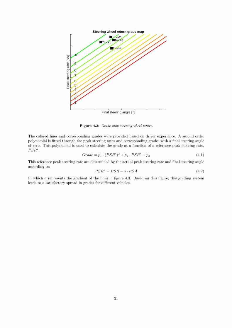
4.3.2 Grading
Figure 4.3 shows the grade map created by the script. A grade is based on the peak steering wheel anglerate and the final steering wheel angle.
20
Final steering angle [°]
Pea
k st
eerin
g ra
te [
°/s]
123456
7
8
9
10
Truck4
Truck3Truck2
Truck1
Steering wheel return grade map
Figure 4.3: Grade map steering wheel return
The colored lines and corresponding grades were provided based on driver experience. A second orderpolynomial is fitted through the peak steering rates and corresponding grades with a final steering angleof zero. This polynomial is used to calculate the grade as a function of a reference peak steering rate,PSR∗:
Grade = p1 · (PSR∗)2 + p2 · PSR∗ + p3 (4.1)
This reference peak steering rate are determined by the actual peak steering rate and final steering angleaccording to:
PSR∗ = PSR− a · FSA (4.2)
In which a represents the gradient of the lines in figure 4.3. Based on this figure, this grading systemleeds to a satisfactory spread in grades for different vehicles.
21
5. Steering ratio
In the new truck program the steering gear design will be partly new. Therefore some parameters forthe ESP Yaw Controller need to be updated. One of these parameters is the total steering ratio fromthe steering wheel to front wheels. The tests needed for determination of the steering ratio were alreadydone for a large number of trucks. The generated data needs to be processed and a report should bewritten which contains the new set of steering ratios.
5.1 Test description
The vehicle is driven on the test track at crawl velocity. After a few seconds straight driving, the steeringwheel is turned at a constant rate to its maximum on one side. When the maximum is reached the wheelis turned in the other direction at the same rate until the maximum on that side is reached. After thisthe steering wheel is returned to the straight forward position. This is repeated several times for eachtruck.
The test was included in the rapid dynamic testing program. This is a test program in which new pro-totypes are subjected to a series of tests while they are only available for two days. The test program isset up efficiently but as the truck also needs to be rigged with the right equipment the actual time slotfor testing is narrow.
Data is gathered from the internal CAN system. Relevant data for this test are the steering wheel angle,the velocity of the front wheels and the yaw rate. This data is analyzed with the use of an existing scriptwhich basics will be explained in the next section.
5.2 Background information
The calculation of the steering ratio is based on the bicycle model introduced in chapter 2. At eachsample point the vehicle velocity, vx, and yaw rate, ωz, are used to calculate the steering radius:
R =vxωz
(5.1)
Combined with the wheel base, L, the Ackermann angle can be determined, see equation 5.2.
δack =L
R(5.2)
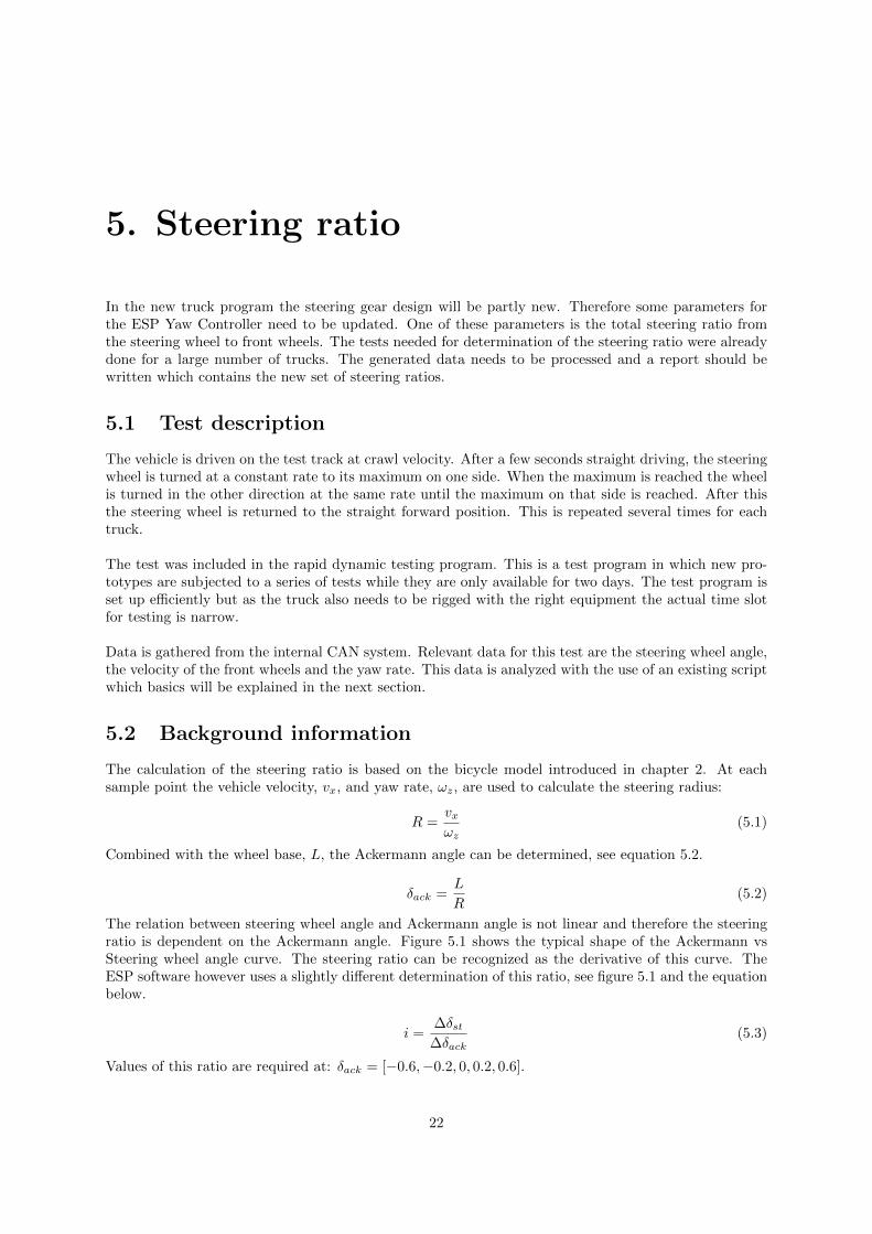
The relation between steering wheel angle and Ackermann angle is not linear and therefore the steeringratio is dependent on the Ackermann angle. Figure 5.1 shows the typical shape of the Ackermann vsSteering wheel angle curve. The steering ratio can be recognized as the derivative of this curve. TheESP software however uses a slightly different determination of this ratio, see figure 5.1 and the equationbelow.
i =∆δst∆δack
(5.3)
Values of this ratio are required at: δack = [−0.6,−0.2, 0, 0.2, 0.6].
22
Figure 5.1: Ackerman angle versus steering wheel angle
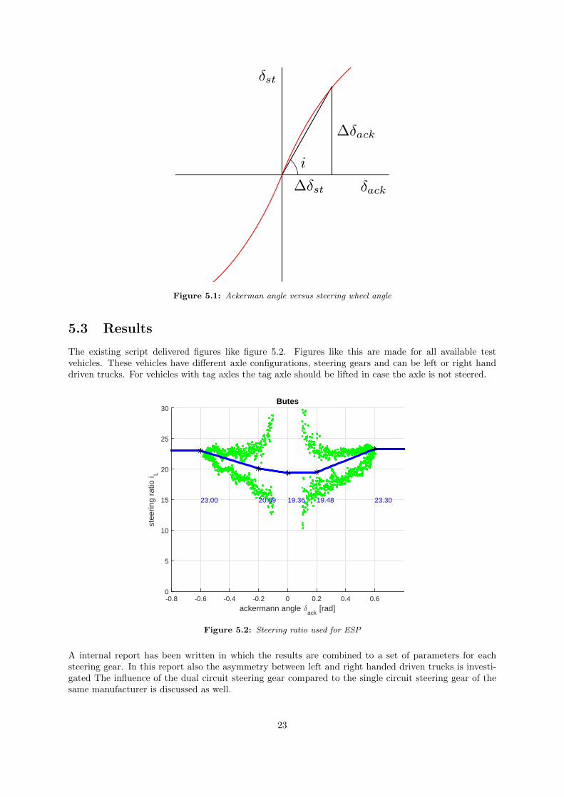
5.3 Results
The existing script delivered figures like figure 5.2. Figures like this are made for all available testvehicles. These vehicles have different axle configurations, steering gears and can be left or right handdriven trucks. For vehicles with tag axles the tag axle should be lifted in case the axle is not steered.
ackermann angle δack
[rad]-0.8 -0.6 -0.4 -0.2 0 0.2 0.4 0.6
stee
ring
ratio
i L
0
5
10
15
20
25
30
23.00 20.09 19.36 19.48 23.30
Butes
Figure 5.2: Steering ratio used for ESP
A internal report has been written in which the results are combined to a set of parameters for eachsteering gear. In this report also the asymmetry between left and right handed driven trucks is investi-gated The influence of the dual circuit steering gear compared to the single circuit steering gear of thesame manufacturer is discussed as well.
23
6. Reflection
In this chapter I will reflect on this internship and working at Scania. I will discuss things that stoodout to me. This whole chapter is written from a personal point of view.
6.1 Company and RTCD
Every day at Scania starts with a fifteen minute morning meeting called ”Daglig styrning”. The agendaof this meeting will differ for each group but the general idea is to discuss accidents or problems fromthe previous day and the planning of the coming day. At RTCD the meetings starts with accidents andthereafter problems or ”Events” from the previous day. Thereafter the progress and planning for eachtest is discussed. The meeting continuous with a round in which each individual states what he or shewill be doing that day. The meeting ends with the workshop layout planning for that day.
Scania uses a system in which an ”Event” will be written in case there is a problem with a product or adesign. This system is copied from the factory. All events are registered in order to keep track of eachproblem. This way one could see if a problem is fixed and in addition it provides an indication of thecurrent status of the departments and the company in general. I knew such systems were in use in theScania factories and at other (automotive) companies, but I was a bit surprised to see these systems arebeing used within R&D as well.
In the company introduction was already stated that Scania always works on improving its processes.This was most apparent in the weekly Forbattringsarbete, or improvement work, meeting. In this meet-ings annoyances and ideas to get rid of these annoyances or improve the functionality of the team arebeing discussed. All ideas are labelled according to effort and benefits. Ideas which could be realizedwith low effort and result in high benefits are assigned as a task to someone in the group. The progressof each person on his or her tasks will be briefly discussed the next meetings until the task is finished.Clearly this meeting and associated tasks do not have the highest priority. However, I suppose it is agood way of improving the work being done by the department. And by using this regulated system allnew ideas will be discussed and no good ideas will be forgotten.
The relation between company and employees was different to me than expected. I expected the workingconditions in Sweden and the Netherlands to be comparable. But I was surprised by the excellenttreatment of Scanias employees considering (flexible) working hours, breaks and career opportunities.However it might sound obvious I would say the safety and well-being of employees is really importantat Scania.
6.2 Communication
The difference between working within a project group of eight people within my bachelor and at ScaniasR&D department consisting of 3500 employees is, off course, huge. The implications were not knownto me at forehand. I was amazed by the effort needed to plan all tests and the number of times thisplanning needed to be revised. Also the difficulty of distributing information and knowledge to eachother was striking to me.
24
For my assignment I did not need to collaborate with other people that much. This was mostly limited tomeetings with the simulation group that were about to use the handling script as well and informal chatswith my supervisor about my progress. At these moments the communication was good according to me.
In my experience there were more difficulties in understanding conversations that were not related tomy assignments. At first I was not acquainted with all terminology and abbreviations used around me.Later on these conversations were more often in Swedish. Hereby I need to mention that I did not askto speak English again that often as many conversations were not related to me at all and I started toglobally understand what these conversations were about.
6.3 What I learned
I certainly improved my Matlab programming skills. I became more familiar with the dealing of largeamounts of data. Also the usage of scripts with this size and this amount of functionalities was new tome. The importance of properly commenting and providing proper documentation to such a programbecame more clear to me.
During this internship and my time in Sweden I did not only improve my English speaking and writingskills. I also got to know the importance of speaking and writing English in a multinational team orcompany in general.
In this internship I learned a lot about vehicle dynamics. Although I had the required theoretical knowl-edge from the courses Dynamics I, Dynamics II, Advanced Dynamics and my work as teaching assistantfor these courses, seeing the application of this knowledge was new to me.
In my studies performing experiments and analysis of test data did not get that much attention. AtRTCD I learned about these topics and got mare interested in this field as well.
There had only been very little practical experience in my studies so far. All in all I would say I learnedmost of just being part in this team and working in a large company.
25
Bibliography
[1] Scania inline Scania, consulted 13-08-2015, no address, excess only at Scania network
[2] Scania global introduction video Scania (2013), consulted 13-08-2015,http://www3.involve.se/SGI2013/
[3] Sheets vehicle dynamics Jolle Ijkema (2012), Scania internal course
[4] Car suspension and handling D. Bastow, G. Howard, J.P. Whitehead (2004), 4th ed.