Evaluation of NASA satellite and modelled temperature data for simulating maize water requirement satisfaction index in the Free State Province of South Africa Mokhele Edmond Moeletsi a,b,⇑ , Sue Walker b a Agricultural Research Council – Institute for Soil, Climate and Water, Private Bag X79, Pretoria 0001, South Africa b Department of Soil, Crop and Climate Sciences, University of the Free State, PO Box 339, Bloemfontein 9300, South Africa article info Article history: Available online 1 September 2012 Keywords: Evapotranspiration Hargreaves Minimum and maximum temperatures Maize WRSI abstract Low density of weather stations and high percentages of missing values of the archived climate data in most places around the world makes it difficult for decision-makers to make meaningful conclusions in natural resource management. In this study, the use of NASA modelled and satellite-derived data was compared with measured minimum and maximum temperatures at selected climate stations in the Free State Province of South Africa. The NASA temperature data-fed Hargreaves evapotranspiration estimate was compared with the Penman–Monteith estimate to obtain regional coefficients for the Free State. The maize water requirement satisfaction index (WRSI) obtained using the NASA temperature data and calibrated Hargreaves equation was evaluated against the WRSI obtained using Penman–Monteith estimate. The data used is mostly from 1999 to 2008. The results of the comparison between measured minimum temperatures and NASA minimum temperatures show overestimation of the NASA values by between a monthly mean of 1.4 °C and 4.1 °C. NASA maximum temperatures seem to underestimate measured temperatures by monthly values ranging from 2.2 to 3.8 °C. NASA-fed Hargreaves equation in its original form underestimates Penman–Monteith evapotranspiration by between 20% and 40% and hence its coefficient was calibrated accordingly. The comparison of the maize WRSI simulated with NASA temperatures showed a good correlation and small deviations from WRSI calculated from mea- sured data. Thus, the use of NASA satellite and modelled data is recommended in the Free State Province in places where there are no meteorological readings, with special consideration of the biasness of the data. Ó 2012 Elsevier Ltd. All rights reserved. 1. Introduction Weather and climate information can be used in many applica- tions ranging from agriculture, forestry, hydrology and engineering purposes (Trapasso, 1986). In the field of agriculture, crop yields are mostly affected by the weather conditions during the growing season and thus most models of crop performance or growth use climate data as their core input (Nonhebel, 1993; Peng et al., 2004). According to Porter and Semenov (2005) and Lobell and Field (2007), slight changes in the mean of a climate variable like temperature can affect growth and development and consequently yield. It is therefore important for governments and other institu- tions to invest in building a good weather station network in sup- port of agricultural research. Proper maintenance of this infrastructure (replacement of malfunctional instruments on time and calibration of sensors) should result in good quality measured data with only isolated missing or faulty data. Accurate climate data enables scientists to better understand local climatology, resulting in increased knowledge of critical factors limiting production. Normally climate data used for modelling in areas without weather stations is taken from neighbouring stations and in some cases there is a small difference in climate in these areas especially when they are not far apart, but in other cases the distances are too large or topography drastically different for one to use neighbour- ing stations. In the latter case, the use of a satellite-derived dataset would help but this data has to be adjusted for the specific region as it can have tendencies of overestimating or underestimating depending on the variable and place. Satellite-derived weather data has been shown to be good enough to provide data in places where there are no weather stations (Chandler et al., 2010). However, the accuracy of the satellite-derived data is still uncer- tain because it is affected by cloud cover, atmospheric aerosols and is mostly of a coarse spatial resolution (Wentz et al., 2000). 1474-7065/$ - see front matter Ó 2012 Elsevier Ltd. All rights reserved. http://dx.doi.org/10.1016/j.pce.2012.08.012 ⇑ Corresponding author. Address: South African Weather Service, Private Bag X097, Pretoria 0001, South Africa. Tel.: +27 12 367 6204; fax: +27 12 367 6031. E-mail addresses: [email protected], [email protected](M.E. Moeletsi). Physics and Chemistry of the Earth 50–52 (2012) 157–164 Contents lists available at SciVerse ScienceDirect Physics and Chemistry of the Earth journal homepage: www.elsevier.com/locate/pce
Transcript
Physics and Chemistry of the Earth 50–52 (2012) 157–164
Contents lists available at SciVerse ScienceDirect
Physics and Chemistry of the Earth
journal homepage: www.elsevier .com/locate /pce
Evaluation of NASA satellite and modelled temperature data for simulatingmaize water requirement satisfaction index in the Free StateProvince of South Africa
Mokhele Edmond Moeletsi a,b,⇑, Sue Walker b
a Agricultural Research Council – Institute for Soil, Climate and Water, Private Bag X79, Pretoria 0001, South Africab Department of Soil, Crop and Climate Sciences, University of the Free State, PO Box 339, Bloemfontein 9300, South Africa
a r t i c l e i n f o a b s t r a c t
Article history:Available online 1 September 2012
Keywords:EvapotranspirationHargreavesMinimum and maximum temperaturesMaizeWRSI
1474-7065/$ - see front matter � 2012 Elsevier Ltd. Ahttp://dx.doi.org/10.1016/j.pce.2012.08.012
⇑ Corresponding author. Address: South African WX097, Pretoria 0001, South Africa. Tel.: +27 12 367 62
Low density of weather stations and high percentages of missing values of the archived climate data inmost places around the world makes it difficult for decision-makers to make meaningful conclusions innatural resource management. In this study, the use of NASA modelled and satellite-derived data wascompared with measured minimum and maximum temperatures at selected climate stations in the FreeState Province of South Africa. The NASA temperature data-fed Hargreaves evapotranspiration estimatewas compared with the Penman–Monteith estimate to obtain regional coefficients for the Free State.The maize water requirement satisfaction index (WRSI) obtained using the NASA temperature dataand calibrated Hargreaves equation was evaluated against the WRSI obtained using Penman–Monteithestimate. The data used is mostly from 1999 to 2008. The results of the comparison between measuredminimum temperatures and NASA minimum temperatures show overestimation of the NASA values bybetween a monthly mean of 1.4 �C and 4.1 �C. NASA maximum temperatures seem to underestimatemeasured temperatures by monthly values ranging from 2.2 to 3.8 �C. NASA-fed Hargreaves equationin its original form underestimates Penman–Monteith evapotranspiration by between 20% and 40%and hence its coefficient was calibrated accordingly. The comparison of the maize WRSI simulated withNASA temperatures showed a good correlation and small deviations from WRSI calculated from mea-sured data. Thus, the use of NASA satellite and modelled data is recommended in the Free State Provincein places where there are no meteorological readings, with special consideration of the biasness of thedata.
� 2012 Elsevier Ltd. All rights reserved.
1. Introduction
Weather and climate information can be used in many applica-tions ranging from agriculture, forestry, hydrology and engineeringpurposes (Trapasso, 1986). In the field of agriculture, crop yieldsare mostly affected by the weather conditions during the growingseason and thus most models of crop performance or growth useclimate data as their core input (Nonhebel, 1993; Peng et al.,2004). According to Porter and Semenov (2005) and Lobell andField (2007), slight changes in the mean of a climate variable liketemperature can affect growth and development and consequentlyyield. It is therefore important for governments and other institu-tions to invest in building a good weather station network in sup-port of agricultural research. Proper maintenance of thisinfrastructure (replacement of malfunctional instruments on time
and calibration of sensors) should result in good quality measureddata with only isolated missing or faulty data. Accurate climatedata enables scientists to better understand local climatology,resulting in increased knowledge of critical factors limitingproduction.
Normally climate data used for modelling in areas withoutweather stations is taken from neighbouring stations and in somecases there is a small difference in climate in these areas especiallywhen they are not far apart, but in other cases the distances are toolarge or topography drastically different for one to use neighbour-ing stations. In the latter case, the use of a satellite-derived datasetwould help but this data has to be adjusted for the specific regionas it can have tendencies of overestimating or underestimatingdepending on the variable and place. Satellite-derived weatherdata has been shown to be good enough to provide data in placeswhere there are no weather stations (Chandler et al., 2010).However, the accuracy of the satellite-derived data is still uncer-tain because it is affected by cloud cover, atmospheric aerosolsand is mostly of a coarse spatial resolution (Wentz et al., 2000).
158 M.E. Moeletsi, S. Walker / Physics and Chemistry of the Earth 50–52 (2012) 157–164
NASA has developed an online database of satellite and model-derived weather data at near real time (NASA, 2007; Chandleret al., 2010). According to White et al. (2008), the data is obtainedfrom the Goddard Earth Observation System (GEOS) assimilationmodel which is derived from a combination of sources, namely:land surface observations; ocean surface observations of surfacepressure; ocean surface sea level pressure and upper winds; sea le-vel winds from space-borne radars; upper-air rawinsondes; upper-air drop sondes; pilot balloons and aircraft winds and lastly remotesensing data from satellites. The data from this web database isprovided on a daily basis dating back to 1983 and weather ele-ments include solar radiation at 2 m, minimum and maximumtemperatures at 2 m, dew point temperature at 2 m, relativehumidity at 2 m, rainfall and wind speed at 10 m (NASA,2007,2010). The data provided is at the spatial resolution of1 � 1� of latitude and longitude (NASA, 2007; Chandler et al.,2010). There has recently been work done on the evaluation oruse of this NASA data in the modelling of wheat phenology (Whiteet al., 2008), the simulation of maize yield potential (Bai et al.,2010) and for the forecasting of extreme fires in Serbia (Westberget al., 2010).
The main aim of this study was threefold: (1) to compare theNASA satellite-derived minimum (Tmin) and maximum tempera-tures (Tmax) with the observed data; (2) to regionally calibratethe Hargreaves equation for estimating Penman–Monteith refer-ence evapotranspiration (ETo) using NASA temperatures; and (3)to evaluate the maize water requirement satisfaction index (WRSI)based on calibrated NASA temperatures versus those obtainedfrom measured meteorological data.
2. Materials and methods
The study was deemed necessary because the majority of thestations in the Free State Province of South Africa only record rain-fall whilst other agro-climate variables like temperature andevapotranspiration are also important. NASA-derived temperaturevalues were evaluated in their original form and with regionaladjustments to determine their usage in places lacking data.Evapotranspiration is crucial in determining whether there is suf-ficient water for a crop to reach maturity and produce grain. Theagrometeorology model mostly used for determining whether acrop’s water requirements are met is the FAO WRSI, which usesrainfall, evapotranspiration, soil water capacity, cultivar lengthand crop coefficients as inputs (Frere and Popov, 1979). All the in-puts are readily available in the study area except evapotranspira-tion which has to be estimated using the Penman–Monteithequation or other empirical models. The Penman–Monteith equa-tion is too data demanding but a previous study (Moeletsi, 2010)shows that the Hargreaves equation (temperature dependent mod-el) has a good association with the Penman–Monteith model hencethis method was used. The Hargreaves model has to be calibratedwith the Penman–Monteith model according to recommendedstandards (Allen et al., 1998; Bautista et al., 2009). NASA-derivedtemperature data were used as input into the Hargreaves model.The values from the calibrated Hargreaves model were used as
input into the WRSI model. The resulting WRSI values were com-pared with the WRSI derived from the Penman–Monteithevapotranspiration.
2.1. Study area
The study area is located in the Free State Province of SouthAfrica. The province is situated between the latitudes 26.6� Southand 30.7� South of the equator and between the longitudes 24.3�East and 29.8� East of the Greenwich meridian. The climate ofthe province is mostly semi-arid except the eastern and northeast-ern parts where humid-subtropical climate is experienced accord-ing to the Köppen climate classification. Average annual rainfallranges from 300 to over 900 mm with more than 70% of the rainfalloccurring in September to April. The topography of the province isdiverse with altitudes of <1200 m in the southern part and>1800 m in the eastern Free State.
2.2. Weather stations
Table 1 shows coordinates and altitudes of the six selectedweather stations used in this study and the temporal coverage ofdata that was used from each weather station for the evaluationexercise, while Fig. 1 shows the distribution of these stations inthe Free State Province. The stations used to demonstrate the com-parison of the measured data and that derived from the NASA web-site were chosen on the basis of data availability and also theirspatial distribution. Stations should have over five years of datafrom 1999 to 2008 with less than 10% missing data and were cho-sen to be evenly distributed over the province to cover different cli-mate and ecological zones.
2.3. Comparison of NASA satellite-derived data with weather stationdata
Daily data for minimum and maximum temperature weredownloaded from the NASA Climatology Resource for Agroclima-tology website for all the automatic stations with sufficient datafrom 1983 to 2008 (http://tinyurl.com/82c3ecb). The website givesan option of adjusting the data to the altitude of the station andthis method was used to download all the data. The measured dailyminimum and maximum temperatures were obtained from theAgricultural Research Council-Institute for Soil, Climate and Water(ARC-ISCW) agroclimate database for all the six stations used toevaluate the NASA satellite-derived data. The mean dekadal valuesat the weather stations were then compared with the NASA long-term mean temperatures. Statistical parameters outlined in Sec-tion 2.6 were calculated for all the stations per month.
2.4. Calibration of evapotranspiration empirical model
Reference evapotranspiration (ET) data is an important input tothe WRSI model used to assess agricultural drought. In order tocalculate WRSI at the stations with long-term rainfall data but withno measured temperature data (which form the bulk of the
Fig. 1. Spatial distribution of the weather stations used in the study.
Fig. 2. Comparison between NASA minimum temperatures and measured minimum temperatures for (a) Bleskop; (b) Bloemfontein; (c) Bothaville; (d) Gladdedrift; (e)Senekal; (f) Welkom.
M.E. Moeletsi, S. Walker / Physics and Chemistry of the Earth 50–52 (2012) 157–164 159
weather stations in the Free State Province), alternative tempera-ture estimates had to be used. ET was then estimated by the Har-greaves model (Eq. (1)) using NASA satellite-derived temperaturedata as input (Hargreaves and Samani, 1985). The Hargreaves mod-
el was used because its correlates better with the Penman–Mon-teith model compared to other empirical models (e.g.Thornthwaite model) used to estimate evapotranspiration usingtemperature data as the only input (Moeletsi, 2010)
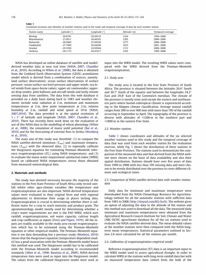
Table 2MBE and RMSE for the NASA minimum temperatures compared with the recorded station data.
Station January February March April May June July August September October November December
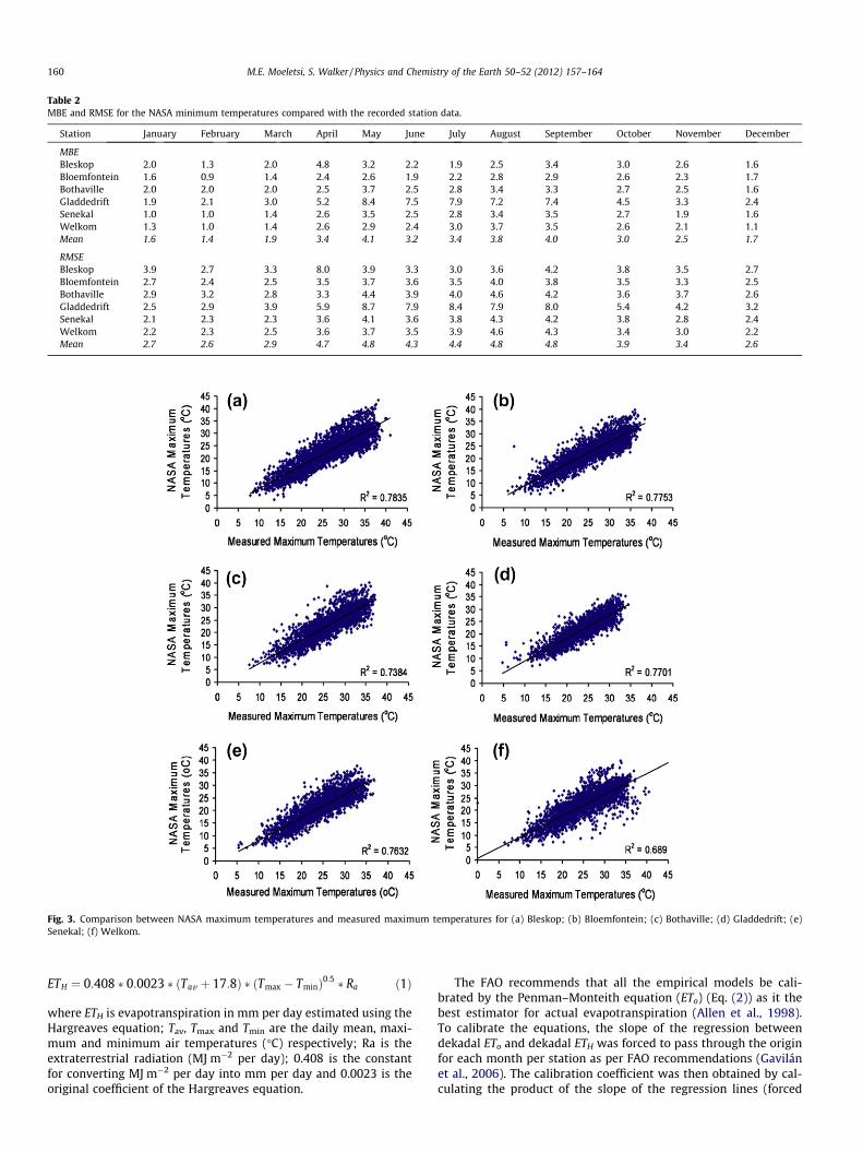
Fig. 3. Comparison between NASA maximum temperatures and measured maximum temperatures for (a) Bleskop; (b) Bloemfontein; (c) Bothaville; (d) Gladdedrift; (e)Senekal; (f) Welkom.
160 M.E. Moeletsi, S. Walker / Physics and Chemistry of the Earth 50–52 (2012) 157–164
ETH ¼ 0:408 � 0:0023 � ðTav þ 17:8Þ � ðTmax � TminÞ0:5 � Ra ð1Þ
where ETH is evapotranspiration in mm per day estimated using theHargreaves equation; Tav, Tmax and Tmin are the daily mean, maxi-mum and minimum air temperatures (�C) respectively; Ra is theextraterrestrial radiation (MJ m�2 per day); 0.408 is the constantfor converting MJ m�2 per day into mm per day and 0.0023 is theoriginal coefficient of the Hargreaves equation.
The FAO recommends that all the empirical models be cali-brated by the Penman–Monteith equation (ETo) (Eq. (2)) as it thebest estimator for actual evapotranspiration (Allen et al., 1998).To calibrate the equations, the slope of the regression betweendekadal ETo and dekadal ETH was forced to pass through the originfor each month per station as per FAO recommendations (Gavilánet al., 2006). The calibration coefficient was then obtained by cal-culating the product of the slope of the regression lines (forced
Table 3MBE and RMSE for the NASA maximum temperatures compared with the recorded station data.
Station January February March April May June July August September October November December
Table 4Statistical summary of the slope of the regression between Penman-Monteith estimate and NASA temperature fed Hargreaves estimate and resultant Hargreaves coefficientobtained from the product of median slope and original Hargreaves coefficient (0.00023) for the 36 stations for the Free State Province in all the months.
Variable January February March April May June July August September October November December
M.E. Moeletsi, S. Walker / Physics and Chemistry of the Earth 50–52 (2012) 157–164 161
to pass at (0,0)) and the original coefficients (Eq. (3)). This slope isequivalent to the ratio of ETo and ETH. A slope of 1 indicates no needfor calibration as the ETH matches the ETo, while a slope of less than1 denotes underestimation of ETo by ETH and a slope exceeding 1denotes overestimation of ETo by ETH. Recalibration of theHargreaves coefficient is required for the last two scenarios.
ETo ¼0:408 � D � ðRn � GÞ þ c 900
Tavþ273
� �u2ðes � eaÞ
Dþ cð1þ 0:34u2Þ
0@
1A ð2Þ
where ETo is in mm day�1; Rn is the net radiation (MJ m�2 per day);G is the soil heat flux (MJ m�2 per day); u2 is the mean wind speedin m s�1; (es–ea) is the saturation vapour pressure deficit (kPa); D isthe slope of the vapour pressure–temperature curve (kPa �C�1) andc is the psychometric constant (kPa �C�1).
CH ¼ slope� 0:0023 ð3Þ
where CH is the new calibration constant for the Hargreaves equa-tion. The resultant calibrated Hargreaves equation is shown in Eq.(4).
ETCH ¼ 0:408 � CH � ðTav þ 17:8Þ � ðT max�T min Þ0:5 � Ra ð4Þ
where ETCH is the calibrated Hargreaves estimate.The selection of the stations used in the regional calibration was
done as follows: weather stations which have over 5 years ofPenman–Monteith evapotranspiration data with less than 10% ofmissing data were chosen. In total 36 weather stations were usedin the determination of regional Hargreaves calibrations. Mediancoefficient adjustment was then obtained from all the 36 stations.
2.5. Comparison of WRSI estimated using NASA satellite-derived datawith WRSI from measured data
For evaluating NASA WRSI versus WRSI calculated from weath-er station data, Tmin and Tmax values data from 1999 to 2008 weredownloaded for all the stations shown in Table 1. The Penman–Monteith evapotranspiration data for the six stations were ob-tained from the ARC-ISCW agroclimate database. The NASA down-loaded temperature data was used to estimate evapotranspirationusing the regionally calibrated Hargreaves coefficient obtainedfrom Section 2.3 on a dekadal basis and these values were com-pared with the Penman–Monteith values.
The WRSI model used in this study operates on a dekadal basis(month is divided into 3 parts: 1st 10 days as dekad 1, 2nd 10 daysas dekad 2 and the remaining days as dekad 3). The analysis wasperformed on medium season maize cultivars with 120-day(12 dekads) growing period. The WRSI water balance model oper-ates on the dekadal steps in which the water stored cannot exceedthe total water-holding capacity after deducting potential evapo-transpiration (Frere and Popov, 1979,1986). Water stored in thesoil profile is added to dekadal rainfall in the following dekad. Ex-cess water is taken as runoff or deep drainage (Senay and Verdin,2003). The WRSI values start from 100 and decrease dekadal bythe proportion of the water deficit over the seasonal potentialevapotranspiration, and it also decreases when the surplus waterexceeds 100 mm (Frere and Popov, 1979,1986).
Measured dekadal rainfall, temperature and Penman–Monteithevapotranspiration data were obtained from the ARC-ISCW agrocli-mate databank while the water-holding capacity of the soil at theweather stations was obtained from the ARC-ISCW soil database.Evapotranspiration data was estimated using the Hargreaves
162 M.E. Moeletsi, S. Walker / Physics and Chemistry of the Earth 50–52 (2012) 157–164
equation calibrated for the Free State region. Standard maize cropcoefficients were used (Allen et al., 1998).
Maize WRSI was then calculated for a maize cultivar that takes120 days to mature during a planting window starting from Octo-ber 1st dekad to January 3rd dekad. Both the Penman–Monteith ETand the regionally calibrated Hargreaves equation ET were used.Statistical parameters in Section 2.6 were used to evaluate thecloseness of the WRSI derived from NASA-adjusted Hargreaves toestimate WRSI calculated from the Penman–Monteith values.
2.6. Statistical analysis
The performance of the NASA-derived dataset was assessed bythe following statistics: coefficient of determination (R2) [deter-mines the correlation between estimated values and measured/ref-erence data], Root Mean Square Error (RMSE) [measures degree ofnon-symmetric error between estimated values and measured/ref-erence data] and Mean Bias Error (MBE) [measures the degree ofunder/over estimation] (Felayi et al., 2011). The Kolmogorov–Smir-nov (KS) similarity test was also used to evaluate the performanceof the NASA weather data to estimate maize WRSI. The decision ismade using the D-value and the p-value which range from 0 to 1.D-value is the maximum deviation between the hypothesizedCumulative Distribution Function (CDF) and the empirical CDFwhile p-value is the critical value at a certain significance level(Wang et al., 2004). If the D-value is much greater than the p-valuethen the statistics of the two datasets do not differ significantly;when the D-value is less than the p-value then the two datasets
Fig. 4. WRSI obtained from NASA data (using Hargreaves Equation for estimating evapBloemfontein; (c) Bothaville; (d) Gladdedrift; (e) Senekal; (f) Welkom.
differ significantly (Van Bockstaele et al., 2006). The KS test embed-ded in the ‘‘Past’’ program was utilized (Hammer et al., 2001).
3. Results and discussion
3.1. Comparison of NASA temperatures with weather station data
NASA dekadal minimum temperatures (Tmin) show a good cor-relation with the recorded data at the six weather stations(Fig. 2). The overall R2 values for all the datasets range from 0.81to 0.88 with an average of 0.85. These high R2 values clearly showthat the NASA minimum temperature data obtained can be used inthe Free State in cases where minimum temperature data at theweather stations are missing or in places where there are noweather stations. MBE values at all the stations show positive biasimplying that the NASA minimum temperature value tends tooverestimate the measured minimum temperature value (Table 2).These MBE values mostly exceed 2 �C with the months from Aprilto September getting relatively higher positive values of up to8.4 �C. RMSE values are less than 4 �C during the main rainfall sea-son (October–March). These RMSE values are mostly around 15% ofthe mean during the summer months while in winter the valuescan reach up to 400% due to very low average minimum tempera-tures of around�0.8 �C in places like Bloemfontein. The differencesmay be attributed to high resolution of the NASA data (1� by 1�).Also, there is a great spatial difference in altitude over an area of100 by 100 km in the Free State. The good correlation obtainedin this study is comparable to those obtained in other areas whichclearly show the worldwide usability of the NASA satellite-derived
otranspiration) compared with the WRSI from measured data for (a) Bleskop; (b)
Table 5MBE, RMSE and KS test results for the NASA temperature fed water requirement satisfaction index (WRSI) compared with WRSI obtained from recorded station data per dekad.
M.E. Moeletsi, S. Walker / Physics and Chemistry of the Earth 50–52 (2012) 157–164 163
weather data (White et al., 2008; Bai et al., 2010). A comparison ofNASA minimum temperature versus the ground data in China re-sulted in underestimation (average bias of �1.4 �C) by NASA tem-peratures while a similar evaluation in the US showedoverestimation (average bias of 1.1 �C) by NASA minimum temper-atures as compared with the measured weather data (White et al.,2008; Bai et al., 2010).
Dekadal NASA maximum temperatures (Tmax) also have a goodagreement with the measured weather station recorded data withthe R2 ranging between 0.69 and 0.79 and averaging 0.76 (Fig. 3).The MBE values are all negative showing that the NASA datasetunderestimated the maximum air temperature in the period1999 to 2008 (Table 3). The MBE values are between �2 �C and�4.3 �C with the average below �2.5 �C for all the months withthe exception of February, September and October. The RMSEranges from 2.5 �C to 5.7 �C with an average of around 4 �C. Rela-tive to the long-term mean, the RMSE is around 13% in the hottestmonths (December and January) while in the coldest months theRMSE makes around 25% of the mean maximum temperatures.The results obtained from other areas also show good correlationbetween NASA maximum temperature and ground data but NASATmax had the tendency of underestimating by 2.4 �C and 2.8 �C inthe US and China respectively (White et al., 2008; Bai et al., 2010).
3.2. Calibration of evapotranspiration model
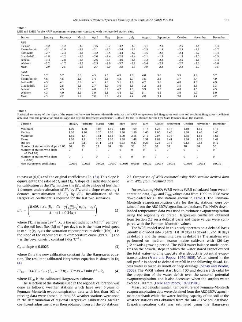
The overall coefficient of determination between Hargreavesestimate using NASA temperatures and Penman–Monteith equa-tion estimate averages 0.84 (n > 3200), ranging from 0.73 to 0.99for all the 36 stations. Results show that the Hargreaves estimatecomputed from NASA temperature can be used to estimate refer-ence evapotranspiration because of the high correlation it has with
the Penman–Monteith estimate (ETo). Even though the correlationis good, the Hargreaves estimate has the tendency of underesti-mating ETo by between 20 (median slope = 1.20) and 60% (medianslope = 1.60), depending on the month (Table 4). Relatively highslopes (ETo/ETH) of 1.5 and 1.6 are obtained in June and August fall-ing within the winter months. During the main agricultural season(November–April) in the Free State Province, underestimation byETH is between 20% and 40%. For all the months, all the stationshave a slope exceeding 1.05 (>5% underestimation) with the excep-tion of February and March where 3 out of 36 and 1 out of 36 sta-tions respectively have their slope close to 1 (0.95–1.05) (Table 4).There are no stations in all the months which show overestimation(slope < 0.95). The standard deviations are mostly less than 0.11 forthe main agricultural season. Relatively high standard deviationsexceeding 0.20 are evident during the winter months (May–Au-gust), coinciding with the months where correlation between ETH
and ETo is the lowest (Moeletsi, 2010) and error estimates of ETH
are the highest (Moeletsi, 2010). A slope that differs from 1 reiter-ates the notion by other researchers (Xu and Singh, 2002; Gavilánet al., 2006) for the coefficient calibration of the Hargreaves empir-ical equation before it can be used at any region. The results of theregionally calibrated coefficient using the median slope are shownin Table 4. The new coefficients range from 0.0028 to 0.0037, dif-fering from the original coefficient of 0.0023 (Hargreaves andSamani, 1985).
3.3. WRSI derived from NASA data versus WRSI obtained frommeasured data
The NASA-derived WRSI values show a good linear correlationwith the WRSI obtained from the measured meteorological data.The R2 values are lowest in Welkom with 0.78; average R2 is 0.87
164 M.E. Moeletsi, S. Walker / Physics and Chemistry of the Earth 50–52 (2012) 157–164
while the highest R2 of 0.92 is obtained at Gladdedrift (Fig. 4). TheMBE values range from �0.3 to 5.4 mm with an average of lessthan 1.5 mm at all six stations for the entire year (Table 5). Theaverage RMSE values are less than 5 mm for all the months. TheKS test at 95% confidence interval for the entire dataset shows thatthe D-values are significantly less than the p-values and thus WRSIcalculated from NASA data is statistically similar to the WRSI ob-tained from measured values for the planting dates of 1st dekadof October–3rd dekad of January (Table 5).
4. Conclusion
In this study minimum and maximum temperatures obtainedfrom the NASA satellite-derived data and measured data werecompared using six weather stations situated in the Free StateProvince of South Africa. NASA satellite-derived data showed agood correlation with the measured weather data. However, theNASA minimum temperatures had the tendency of overestimatingmeasured values while NASA maximum temperatures tended tounderestimate as compared to data recorded at the weather sta-tions. The regional calibration of the Hargreaves equation to esti-mate Penman–Monteith evapotranspiration also resulted in WRSIvalues that resemble WRSI obtained from the measured values.Hence the use of NASA temperature data is recommended in theFree State Province to drive models important for policy or decisionmaking processes especially where there are no climate records ormissing values, taking into consideration the biasness of the data.
Acknowledgements
This study was supported by the Agricultural Research Council-Institute for Soil, Climate and Water (Project Number GW57/007).The authors are grateful to the late Mr. Prospard Gondwe of theZambia Meteorological Services for helping in identifying anddownloading the NASA dataset.
References
Allen, R.G., Pereira, L.S., Raes, D., Smith, M., 1998. Crop evapotranspiration:guidelines for computing crop water requirements. FAO Irrigation andDrainage Paper 55. Rome, Italy.
Bai, J., Chen, X., Dobermman, A., Yang, H., Cassman, K.G., Zhang, F., 2010. Evaluationof NASA satellite- and model-derived weather data for simulation of maizeyield potential in China. Agronomy Journal 102 (1), 9–16.
Bautista, F., Bautista, D., Delgado-Carranza, C., 2009. Calibration of the equations ofHargreaves and Thornthwaite to estimate the potential evapotranspiration insemi-arid and subhumid tropical climates for regional applications. Atmósfera22 (4), 331–348.
Chandler, W.S., Hoell, J.M., Westberg, D., Whitlock, C.H., Zhang, T. and Stackhouse Jr.,P.W., 2010. Near real-time global radiation and meteorology web services
available from NASA. (retrieved on 02.08.10) <http://www.ases.org/papers/120.pdf>.
Felayi, E.O., Rabiu, A.B., Teliat, R.O., 2011. Correlations to estimate monthly mean ofdaily diffuse solar radiation in some selected cities in Nigeria. Advances inApplied Science Research 2 (4), 480–490.
Frere, M., Popov, G., 1979. Agrometeorological crop monitoring and forecasting. FAOplant production and protection paper 17, p. 64.
Frere, M., Popov, G., 1986. Early agrometeorological crop yield assessment. FAOplant production and protection paper 73, p. 144.
Gavilán, P., Lorite, I.J., Tornero, S., Berengena, J., 2006. Regional calibration ofHargreaves equation for estimating reference ET in a semiarid environment.Agricultural Water Management 81, 257–281.
Hammer, ., Harper, D.A.T., Ryan, P.D., 2001. PAST: paleontological statistics softwarepackage for education and data analysis. Palaeontologia Electronica 4 (1), 9.
Lobell, D.B., Field, C.B., 2007. Global scale climate–crop yield relationships and theimpacts of recent warming. Environmental Research Letters 2, 1–7.
Moeletsi, M.E., 2010. Agroclimatological risk assessment of rain-fed maizeproduction for the Free State Province of South Africa. PhD thesis.Department of Soil, Crop and Climate Sciences, University of the Free State,Bloemfontein.
NASA, 2007. NASA Surface Meteorology and Solar Energy: Methodology. (lastviewed 09.07.09) <http://www.ceoe.udel.edu/windpower/ResourceMap/SSE_Methodology.pdf>.
NASA, 2010. NASA Climatology Resource for Agroclimatology Daily Averaged Data(Evaluation Version). (last viewed 23.08.09) <http://earthwww.larc.nasa.gov/cgi-bin/cgiwrap/solar/[email protected]>.
Nonhebel, S.I., 1993. The importance of weather data in crop growth simulationmodels and assessment of climatic change effects. PhD thesis, WageningenUniversity, 6701 BH Wageningen, Netherlands.
Peng, S., Huang, J., Sheehy, J.E., Laza, R.C., Visperas, R.M., Zhong, X., Centeno, G.S.,Kush, S.K., Cassman, K.G., 2004. Rice yields decline with higher nighttemperature from global warming. In: Proceedings of the National Academyof Sciences of the United States of America.
Porter, J.R., Semenov, M.A., 2005. Crop responses to climate variation. PhilosophicalTransactions of The Royal Society B 360, 2021–2035.
Senay, G.B., Verdin, J., 2003. Characteristization of yield reduction in Ethiopia usinga GIS-based crop water balance model. Canadian Journal of Remote Sensingan29 (6), 687–692.
Trapasso, L.M., 1986. Meteorological data acquisitions in Ecuador, South America:problems and solutions. GeoJournal 12 (1), 89–94.
Van Bockstaele, F., Janssens, A., Piette, A., Callewaert, F., Pede, V., Offner, F.,Verhasselt, B., Philippe, J., 2006. Kolmogorov–Smirnov statistical test foranalysis of ZAP-70 expression in B-CLL, compared with quantitative PCR andIgVH mutation status. Cytometry Part B (Clinical Cytometery) 70B, 302–308.
Wang, Y., Yam, R.C.M., Zuo, M.J., 2004. A multi-criterion evaluation approach toselection of the best statistical distribution. Computers & Industrial Engineering47 (2–3), 165–180.
Wentz, F.J., Gentemann, C., Smith, D., Cheiton, D., 2000. Satellite measurements ofsea surface temperature through clouds. Science 288 (5467), 847–850.
Westberg, D., Soja, A., Stackhouse Jr., P.W., 2010. Linking satellite-derived firecounts to satellite-derived weather data in fire prediction models to forecastextreme fires in Siberia. Geophysical Research Abstracts 12, EGU2010-5597.
White, J.F., Hoogenboom, G., Stackhouse Jr., P.W., Hoell, J.M., 2008. Evaluation ofNASA satellite- and assimilation model-derived long-term daily temperaturedata over the continental US. Agricultural and Forest Meteorology 148, 1574–1584.
Xu, C.Y., Singh, V.P., 2002. Cross comparison of empirical equations for calculatingpotential evapotranspiration with data from Switzerland. Water ResourceManagement 16, 197–219.