42
Evaluation of segmentation
| Date post: | 15-Dec-2015 |
| Category: |
Documents |
| Upload: | ricardo-kellum |
| View: | 231 times |
| Download: | 2 times |
Evaluation of segmentation

Example

Reference standard & segmentation
Segmentation performance
• Qualitative/subjective evaluation the easy way out, sometimes the only option
• Quantitative evaluation preferable in general• A wild variety of performance measures exists• Many measures are applicable outside the
segmentation domain as well• Focus here is on two class problems
Some terms
• Ground truth = the real thing• Gold standard = the best we can get• Bronze standard = gold standard with limitations• Reference standard = preferred term for gold
standard in the medical community
What to evaluate?
• Without reference standard, subjective or qualitative evaluation is hard to avoid
• Region/pixel based comparisons• Border/surface comparisons• (a selection of) Points• Global performance measures versus local
measures
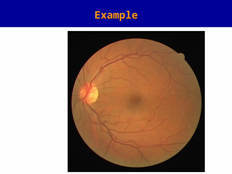
Example
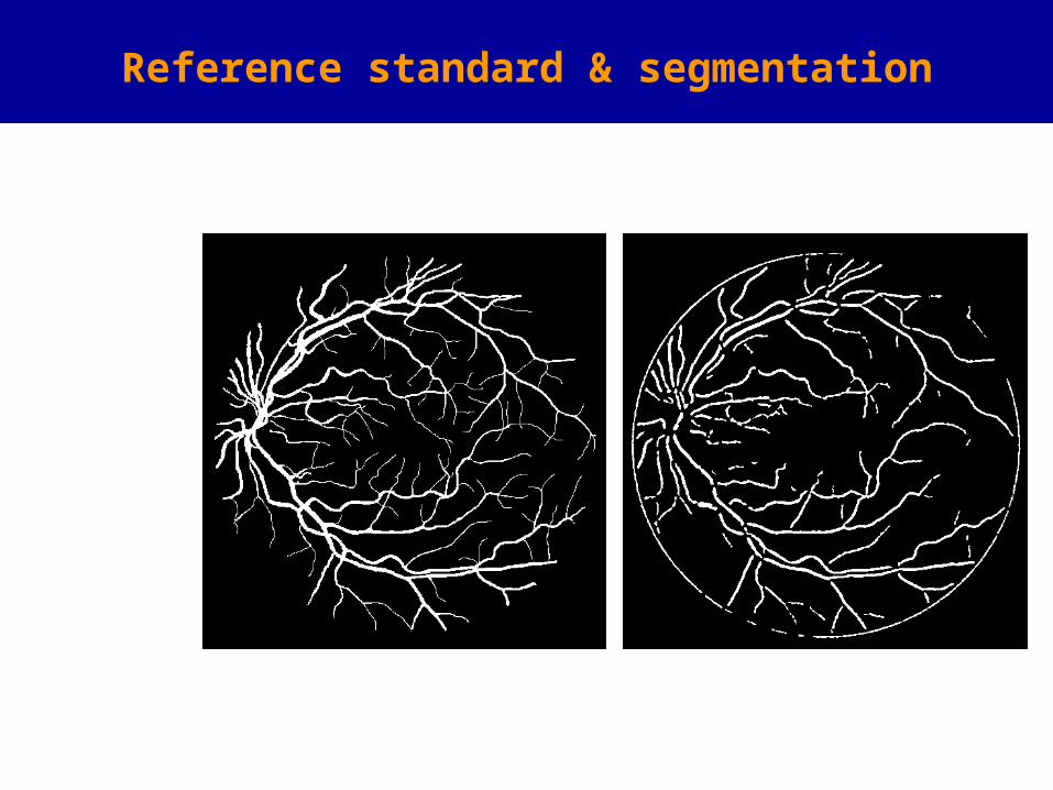
Reference standard & segmentation
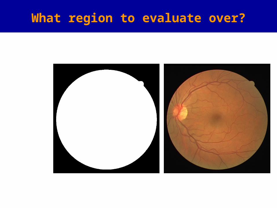
What region to evaluate over?
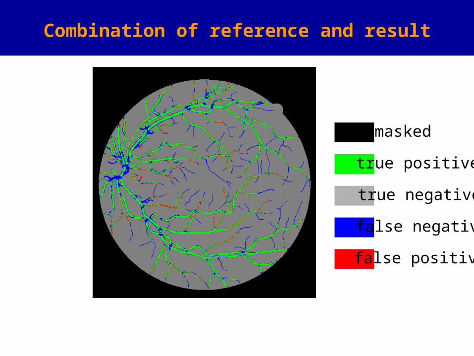
Combination of reference and result
masked
true positive
true negative
false negative
false positive
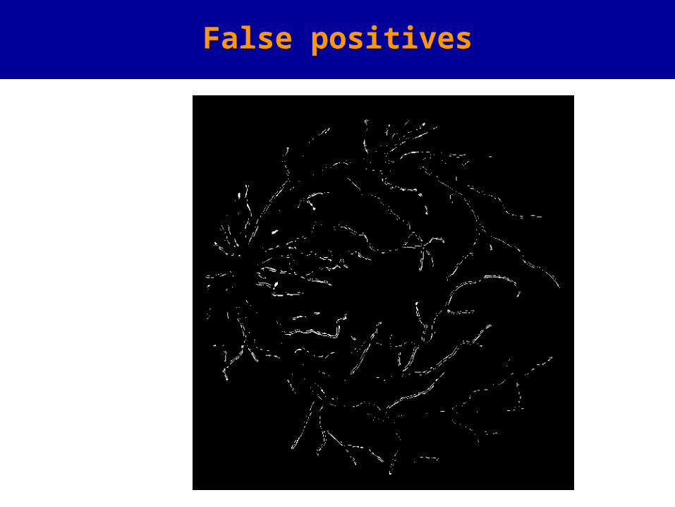
False positives
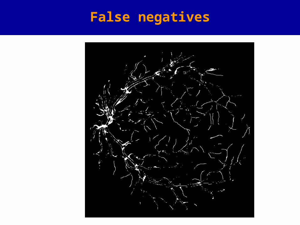
False negatives
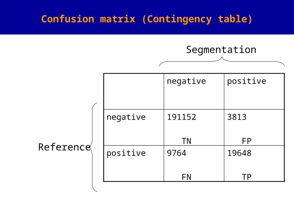
Confusion matrix (Contingency table)
Segmentation
Reference
negative positive
negative 191152 TN
3813 FP
positive 9764 FN
19648 TP
Do not get confused!
• False positives are actually negative• False negatives are actually positives

Confusion matrix (Contingency table)
Segmentation
Reference
negative positive
negative .852 TN
.017 FP
positive .044 FN
.088 TP
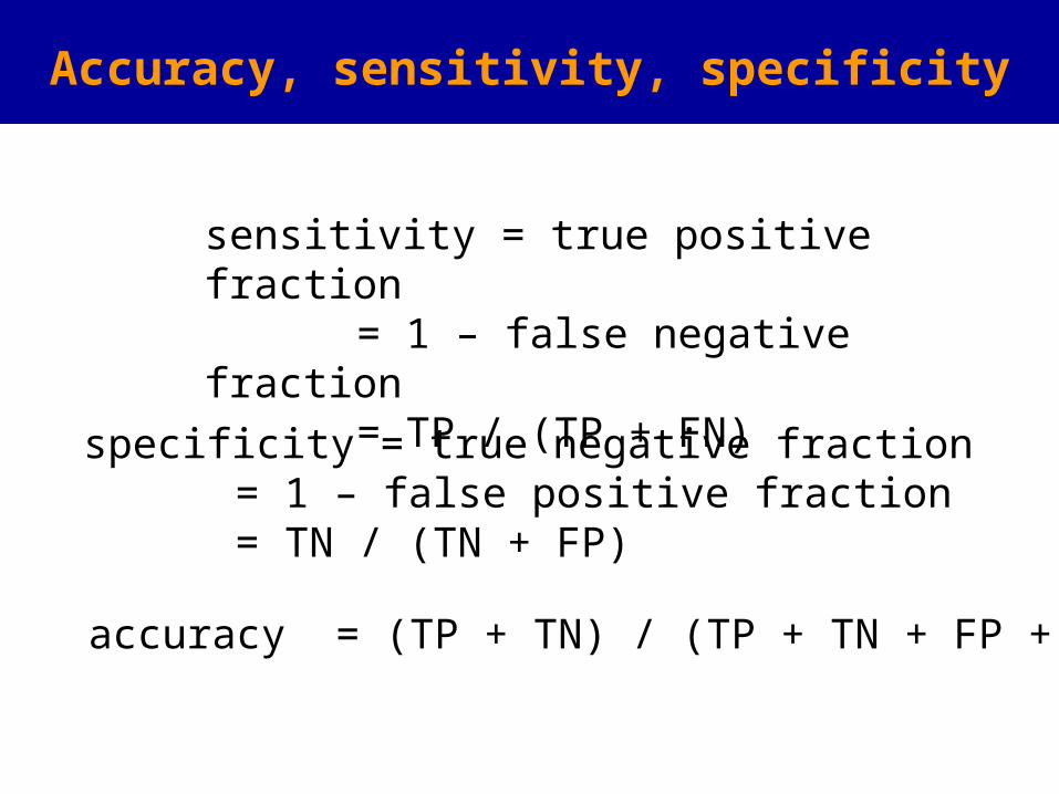
Accuracy, sensitivity, specificity
sensitivity = true positive fraction = 1 – false negative fraction = TP / (TP + FN)
specificity = true negative fraction = 1 – false positive fraction = TN / (TN + FP)
accuracy = (TP + TN) / (TP + TN + FP + FN)
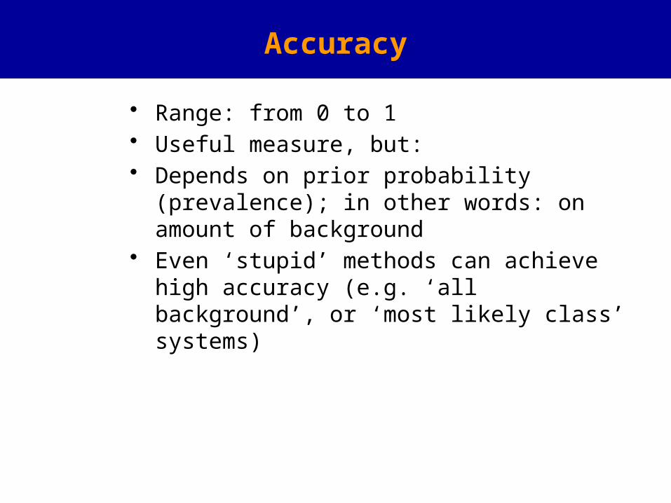
Accuracy
• Range: from 0 to 1• Useful measure, but:• Depends on prior probability (prevalence); in
other words: on amount of background• Even ‘stupid’ methods can achieve high
accuracy (e.g. ‘all background’, or ‘most likely class’ systems)
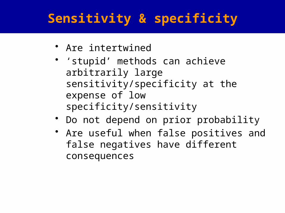
Sensitivity & specificity
• Are intertwined• ‘stupid’ methods can achieve arbitrarily large
sensitivity/specificity at the expense of low specificity/sensitivity
• Do not depend on prior probability• Are useful when false positives and false
negatives have different consequences
N PN
N N
NN
P P
P
PP
PPNN
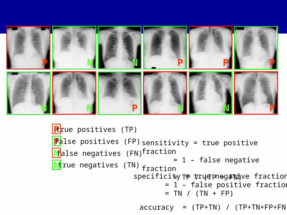
true positives (TP)
false positives (FP)
false negatives (FN)
true negatives (TN)
sensitivity = true positive fraction = 1 – false negative fraction = TP / (TP + FN)
specificity = true negative fraction = 1 – false positive fraction = TN / (TN + FP)
accuracy = (TP+TN) / (TP+TN+FP+FN)
N PN
N N
NN
P P
P
PP
PPNN
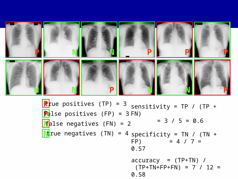
true positives (TP) = 3
false positives (FP) = 3
false negatives (FN) = 2
true negatives (TN) = 4
sensitivity = TP / (TP + FN) = 3 / 5 = 0.6
specificity = TN / (TN + FP) = 4 / 7 = 0.57
accuracy = (TP+TN) / (TP+TN+FP+FN) = 7 / 12 = 0.58
N PN
N N
NN
P P
P
PP
PP
NN
= 3
= 3
= 2
= 4
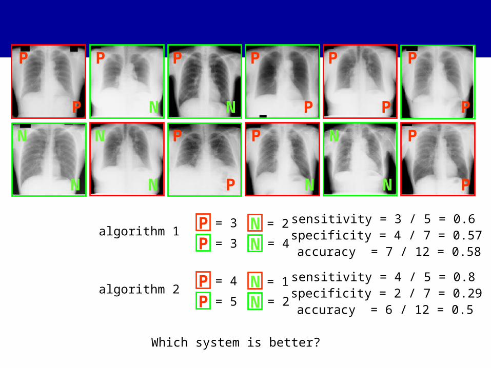
sensitivity = 3 / 5 = 0.6specificity = 4 / 7 = 0.57accuracy = 7 / 12 = 0.58
algorithm 1
N PN
P P
NP
P P
P
PP
PP
NN
= 4
= 5
= 1
= 2
sensitivity = 4 / 5 = 0.8specificity = 2 / 7 = 0.29accuracy = 6 / 12 = 0.5
algorithm 2
Which system is better?
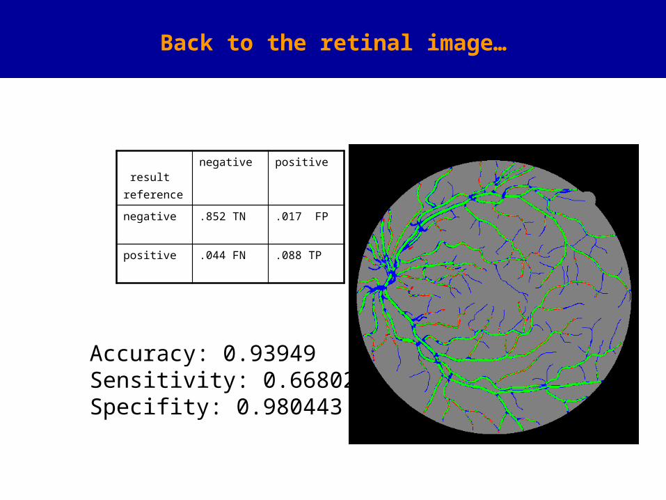
Back to the retinal image…
resultreference
negative positive
negative .852 TN .017 FP
positive .044 FN .088 TP
Accuracy: 0.93949Sensitivity: 0.668027Specifity: 0.980443
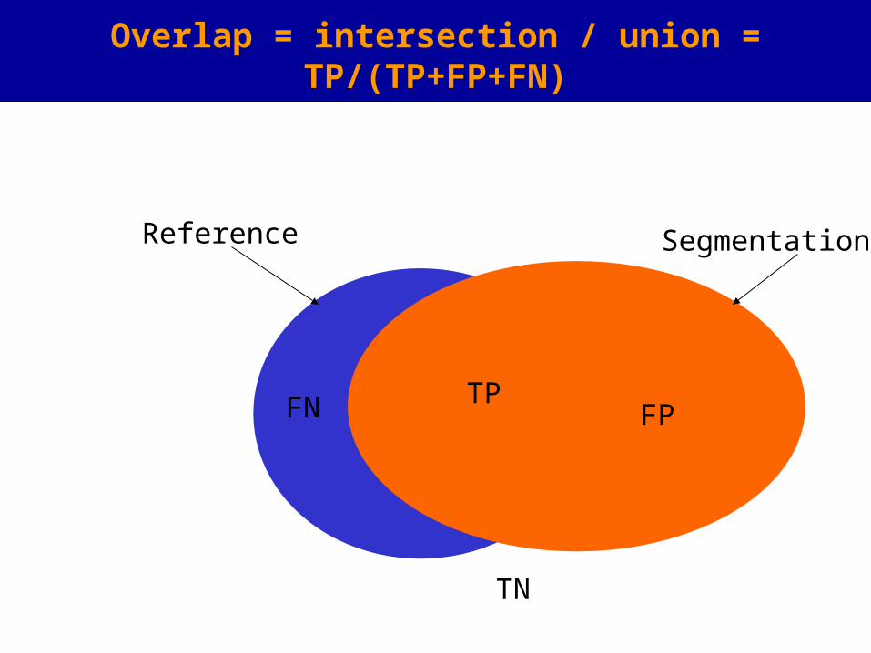
Overlap = intersection / union = TP/(TP+FP+FN)
TPFN FP
TN
Reference Segmentation
Overlap
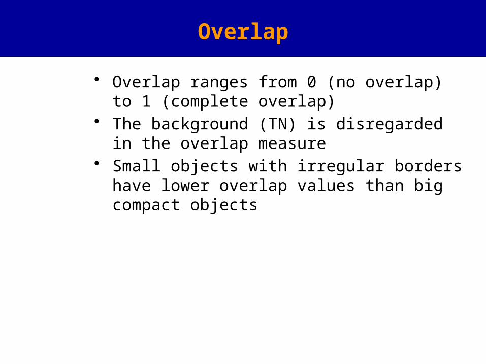
• Overlap ranges from 0 (no overlap) to 1 (complete overlap)
• The background (TN) is disregarded in the overlap measure
• Small objects with irregular borders have lower overlap values than big compact objects
Kappa
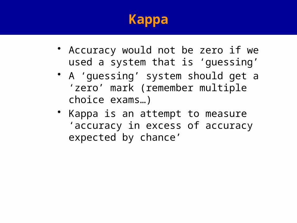
• Accuracy would not be zero if we used a system that is ‘guessing’
• A ‘guessing’ system should get a ‘zero’ mark (remember multiple choice exams…)
• Kappa is an attempt to measure ‘accuracy in excess of accuracy expected by chance’
Kappa
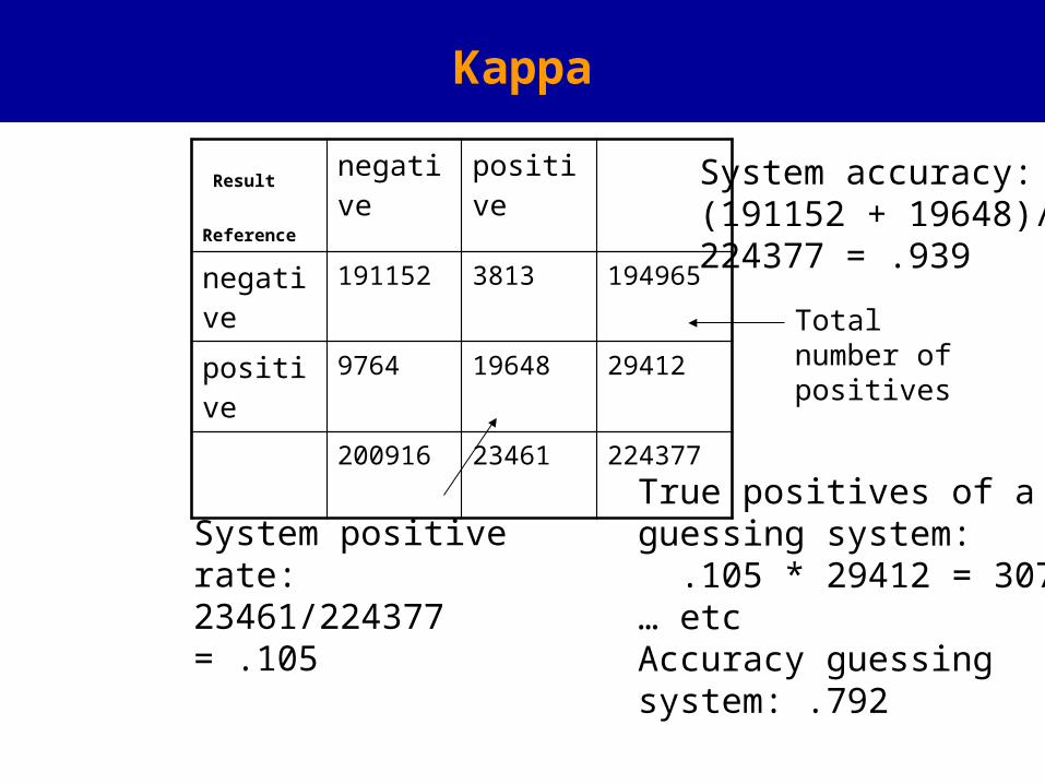
Result
Reference
negative positive
negative 191152 3813 194965
positive 9764 19648 29412
200916 23461 224377
System positive rate:23461/224377 = .105
Total number of positives
True positives of a guessing system: .105 * 29412 = 3075… etcAccuracy guessingsystem: .792
System accuracy:(191152 + 19648)/ 224377 = .939
Kappa
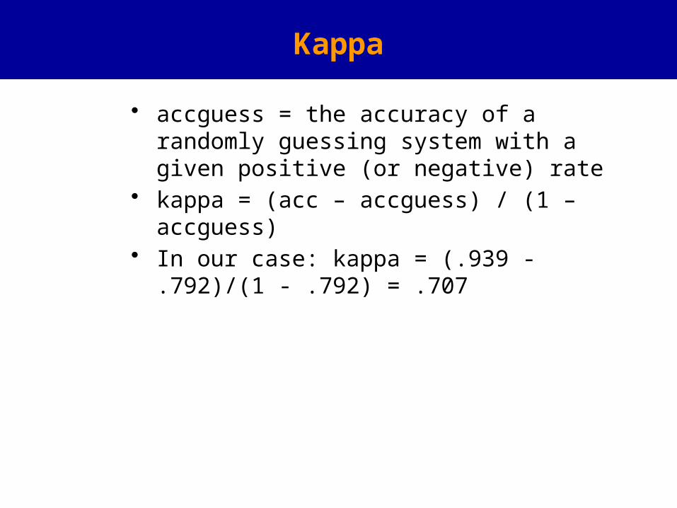
• accguess = the accuracy of a randomly guessing system with a given positive (or negative) rate
• kappa = (acc – accguess) / (1 – accguess)• In our case: kappa = (.939 - .792)/(1 - .792)
= .707
Kappa
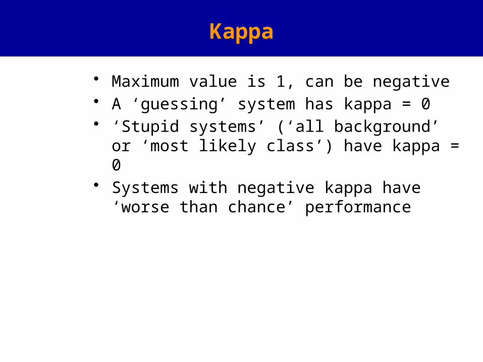
• Maximum value is 1, can be negative• A ‘guessing’ system has kappa = 0• ‘Stupid systems’ (‘all background’ or ‘most likely
class’) have kappa = 0• Systems with negative kappa have ‘worse than
chance’ performance
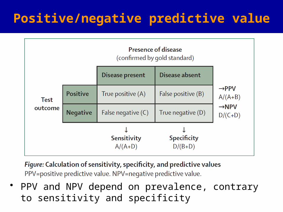
Positive/negative predictive value
• PPV and NPV depend on prevalence, contrary to sensitivity and specificity
ROC analysis
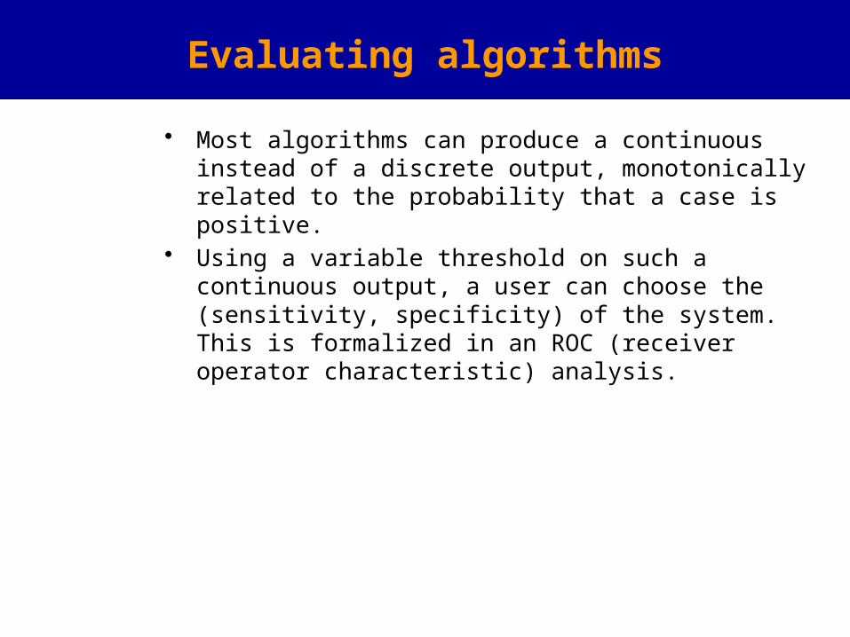
Evaluating algorithms
• Most algorithms can produce a continuous instead of a discrete output, monotonically related to the probability that a case is positive.
• Using a variable threshold on such a continuous output, a user can choose the (sensitivity, specificity) of the system. This is formalized in an ROC (receiver operator characteristic) analysis.
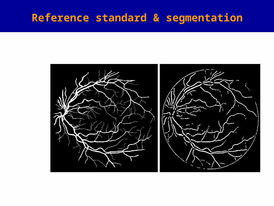
Reference standard & segmentation
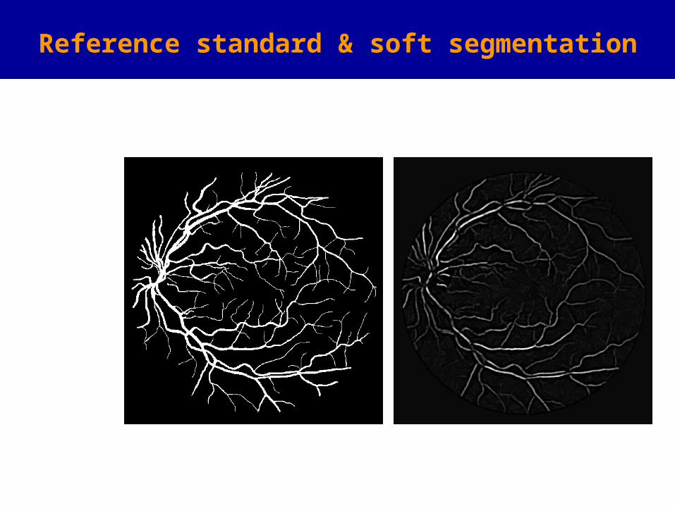
Reference standard & soft segmentation
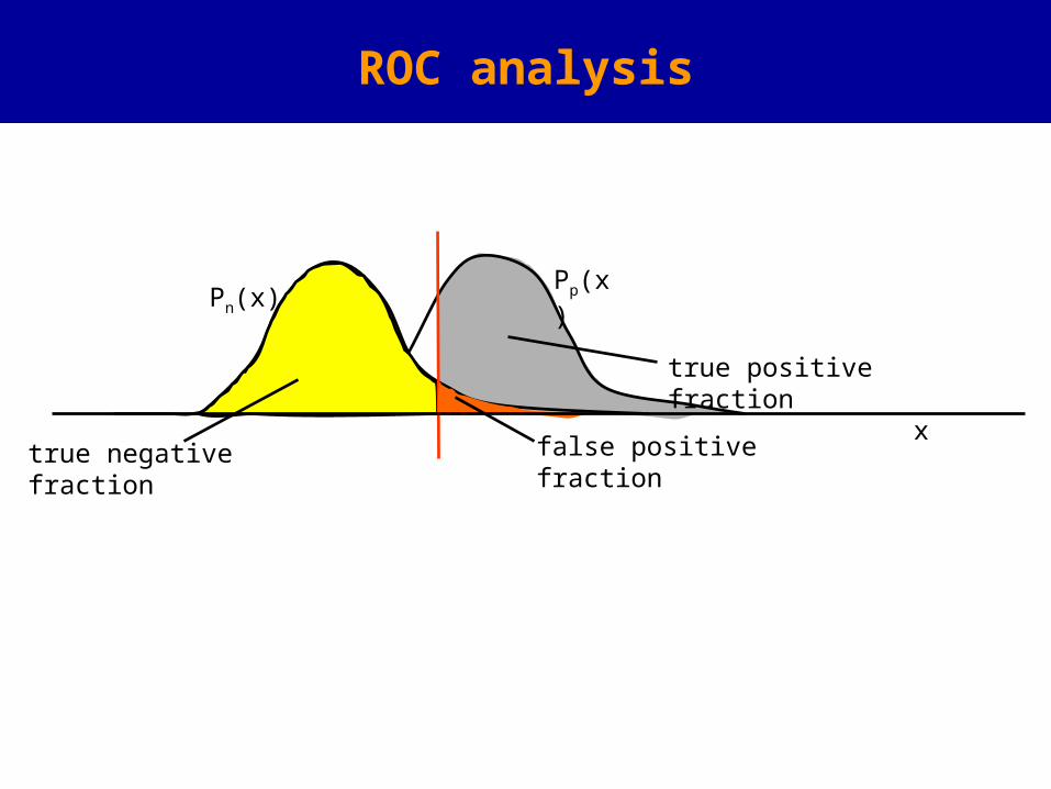
ROC analysis
Pn(x)Pp(x)
x
true positive fraction
true negative fraction false positive fraction
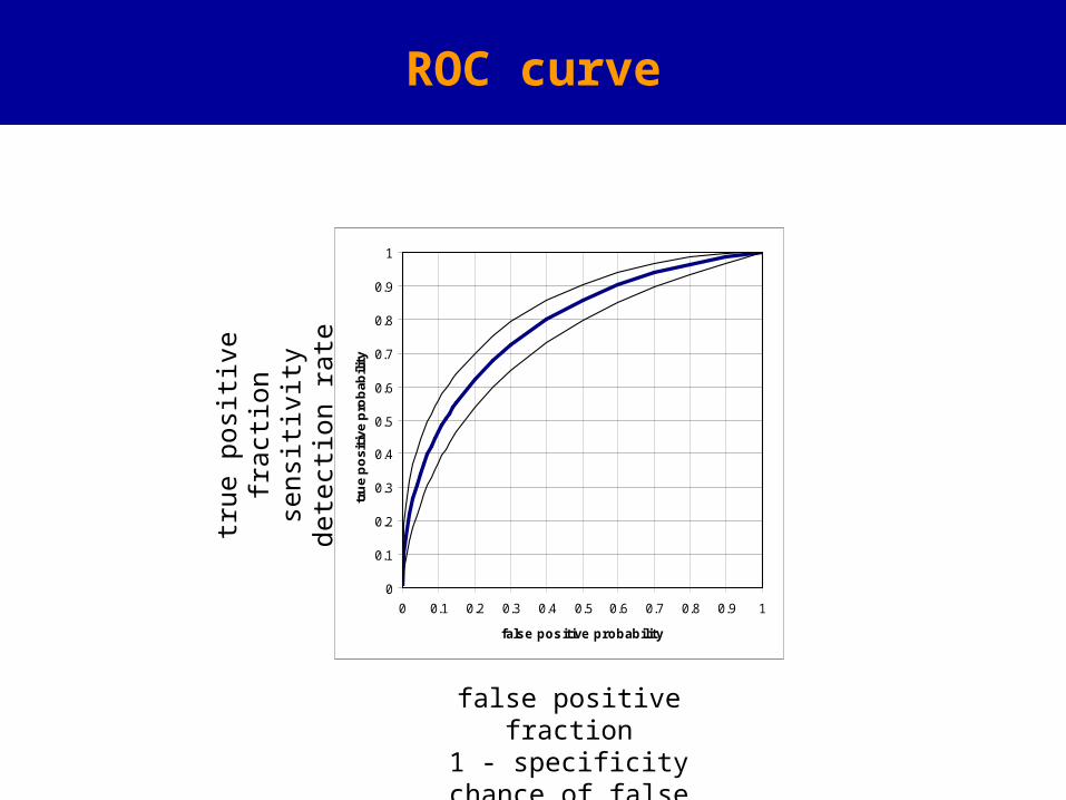
ROC curve
0
0.1
0.2
0.3
0.4
0.5
0.6
0.7
0.8
0.9
1
0 0.1 0.2 0.3 0.4 0.5 0.6 0.7 0.8 0.9 1
false pos itive probability
tru
e p
osi
tive
pro
bab
ility
true p
osi
tive f
ract
ion
sensi
tivit
ydete
ctio
n r
ate
false positive fraction1 - specificity
chance of false alarm
ROC curves
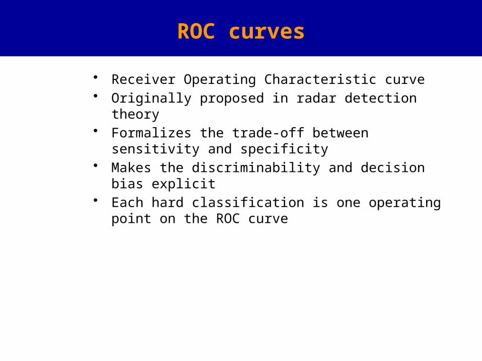
• Receiver Operating Characteristic curve• Originally proposed in radar detection theory• Formalizes the trade-off between sensitivity and specificity• Makes the discriminability and decision bias explicit• Each hard classification is one operating point on the ROC
curve
ROC curves
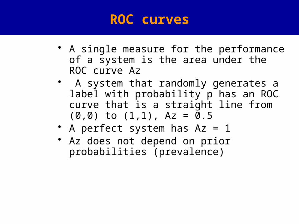
• A single measure for the performance of a system is the area under the ROC curve Az
• A system that randomly generates a label with probability p has an ROC curve that is a straight line from (0,0) to (1,1), Az = 0.5
• A perfect system has Az = 1• Az does not depend on prior probabilities
(prevalence)
ROC curves
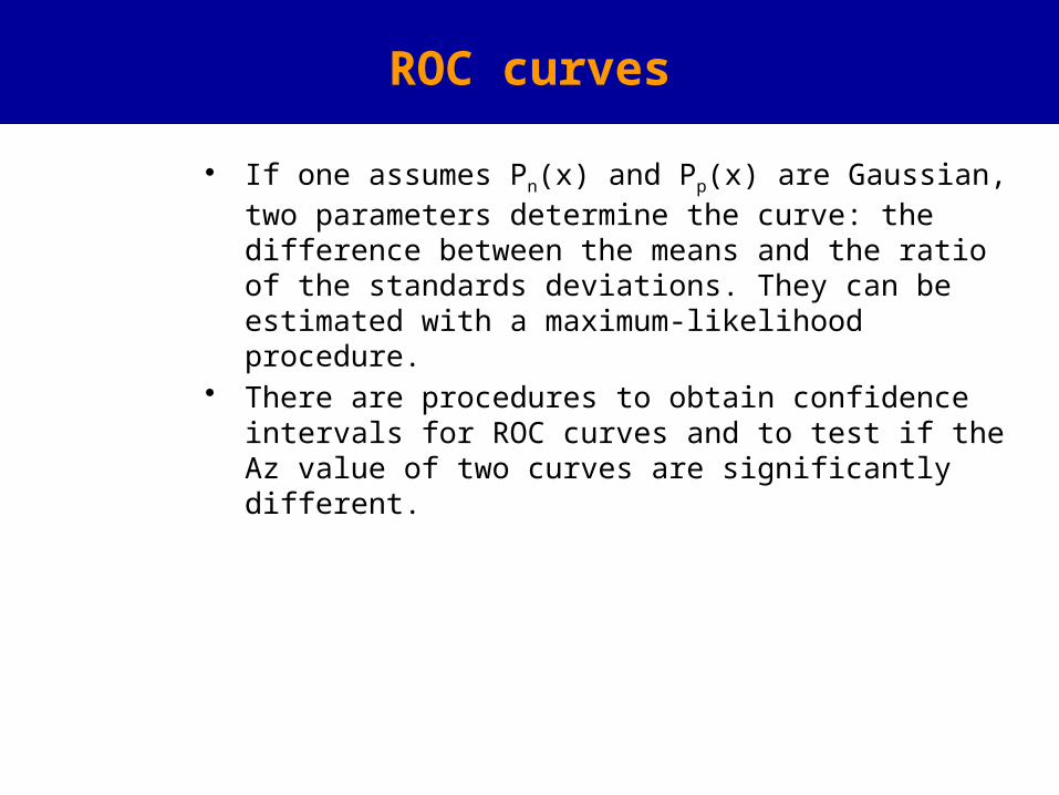
• If one assumes Pn(x) and Pp(x) are Gaussian, two parameters determine the curve: the difference between the means and the ratio of the standards deviations. They can be estimated with a maximum-likelihood procedure.
• There are procedures to obtain confidence intervals for ROC curves and to test if the Az value of two curves are significantly different.
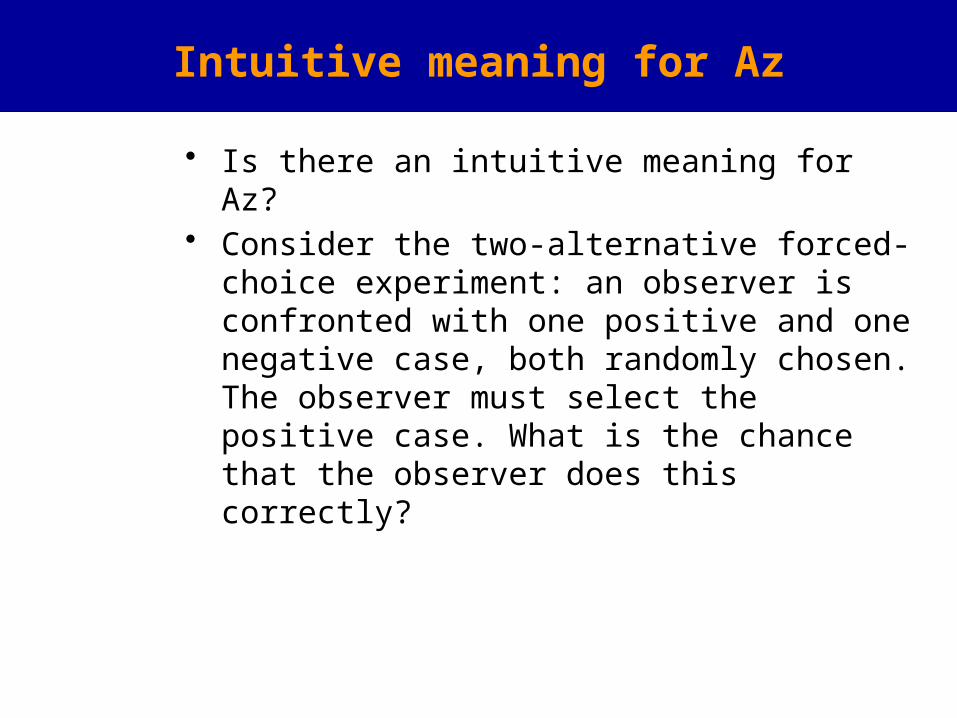
Intuitive meaning for Az
• Is there an intuitive meaning for Az?• Consider the two-alternative forced-choice
experiment: an observer is confronted with one positive and one negative case, both randomly chosen. The observer must select the positive case. What is the chance that the observer does this correctly?
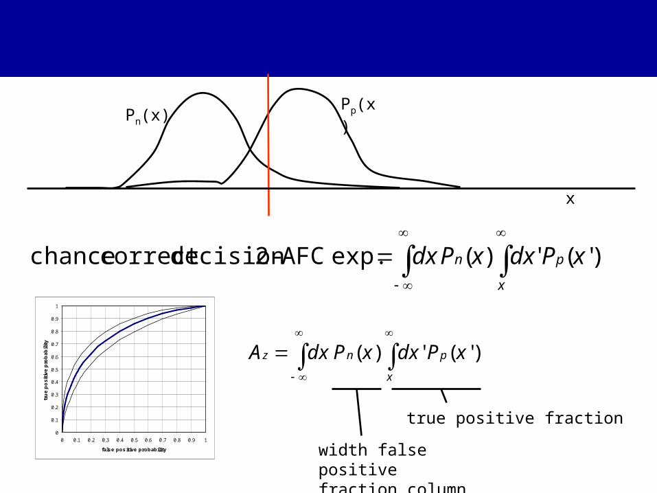
Pn(x)Pp(x)
x
true positive fraction
x
pnz xPdxxPdxA )'( ' )(
0
0.1
0.2
0.3
0.4
0.5
0.6
0.7
0.8
0.9
1
0 0.1 0.2 0.3 0.4 0.5 0.6 0.7 0.8 0.9 1
false positive probability
tru
e p
os
itiv
e p
rob
ab
ilit
y
width false positive fraction column
x
pn xPdxxPdx )'( ' )( exp. AFC-2decision correct chance
Az as a segmentation performance measure
• Ranges from 0.5 to 1• Soft labeling is required (not easy for humans in
segmentation)• Independent of system threshold (operating
point) and prevalence (priors)• Depends on ‘amount of background’ though!
Summary
• Various pixel-based measures were considered for two class, hard (binary) classification results:– Accuracy– Sensitivity, specificity– Overlap– Kappa
• ROC


![LNCS 8694 - Joint Semantic Segmentation and 3D ...lif/HybridSFM-ECCV2014.pdf · Semantic segmentation can be used to estimate 3D information [22,10,25]. For example, Liu et al. [22]](https://static.documents.pub/doc/80x56/5f10ba9d7e708231d44a889d/lncs-8694-joint-semantic-segmentation-and-3d-lifhybridsfm-eccv2014pdf.jpg)


