Evaluation of the effects of design choices on surface mounted

Aino Manninen

Evaluation of the effects of design choices on surface

mounted permanent magnet machines using an

analytical dimensioning tool

Sähkötekniikan korkeakoulu

Diplomityö, joka on jätetty opinnäytteenä tarkastettavaksi

diplomi-insinöörin tutkintoa varten Espoossa 25.5.2012.

Työn valvoja:

Prof. Antero Arkkio

Työn ohjaajat:

TkT Jenni Pippuri, tutk. prof. Kari Tammi

A’’ Aalto-yliopisto

Sähkötekniikan

korkeakoulu

AALTO-YLIOPISTO

SÄHKÖTEKNIIKAN

KORKEAKOULU

DIPLOMITYÖN

TIIVISTELMÄ

Tekijä: Aino Manninen

Työn nimi: Kestomagnetoidun tahtikoneen suunnitteluparametrien vaikutuksen

arviointi analyyttisen mitoitustyökalun avulla

Päivämäärä: 25.5.2012 Kieli: englanti Sivumäärä: 76 + 5

Sähkötekniikan laitos

Professuuri: Sähkömekaniikka

Koodi: S-17

Valvoja: prof. Antero Arkkio

Ohjaajat: TkT Jenni Pippuri, tutk. prof. Kari Tammi

Tämä diplomityö käsittelee kestomagnetoidun tahtikoneen suunnitteluparametrien

kuten esimerkiksi napapariluvun tai ilmavälivuontiheyden vaikutusta koneen

ominaisuuksiin. Työssä toteutettiin analyyttisiin laskentakaavoihin perustuva

mitoitustyökalu pintamagneettikoneelle, jonka staattorissa on yksikerroskäämitys.

Tämän avulla pyrittiin selvittämään, miten eri suunnitteluparametrien valinta

vaikuttaa koneen hyötysuhteeseen, tehokertoimeen, kokoon sekä

kestomagneettimateriaalin määrään. Erityisesti pyrittiin selvittämään, miten koneesta

voitaisiin saada mahdollisimman kompakti.

Toteutettu mitoitustyökalu verifioitiin vertaamalla sen antamia tuloksia

elementtimenetelmällä laskettuihin tuloksiin. Esimerkkinä työkalua testattiin

kuvitteellisen 22 kW teollisuuspumpun suunnittelemiseen. Suunnitteluparametrien

vaikutuksen selvittämiseksi työkalulla laskettiin joukko erilaisia mitoituksia valitulle

koneelle. Havaittiin, että koneesta saadaan kevyempi kasvattamalla napaparilukua,

virran tiheyttä staattorikäämityksessä sekä magneettivuon tiheyttä staattorissa.

Tällöin haittapuolena oli hyötysuhteen huononeminen.

Avainsanat: kestomagnetoitu tahtikone - suunnittelu - mitoitustyökalu

AALTO-UNIVERSITY

SCHOOL OF ELECTRICAL

ENGINEERING

ABSTRACT OF THE

MASTER’S THESIS

Author: Aino Manninen

Title: Evaluation of the effects of design choices on surface mounted permanent

magnet machines using an analytical dimensioning tool

Date: 25.5.2012 Language: English Number of pages: 76 + 5

Department of Electrical Engineering

Professorship: Electromechanics

Code: S-17

Supervisor: Prof. Antero Arkkio

Instructors: D.Sc. (Tech.) Jenni Pippuri, Res. Prof. Kari Tammi

During the design of a permanent magnet machine, there are several parameters that

can be chosen quite freely. These parameters affect the machine properties such as

efficiency, power factor, size and volume of the permanent magnets. By choosing

these parameters well, a compact design is obtained. The purpose of this Master’s

Thesis is to evaluate the effect of different design parameters. The study concentrates

on surface mounted permanent magnet machines with single layer winding in the

stator.

To be able to evaluate the effect of the design choices, a dimensioning tool is

implemented with MATLAB software. The tool is based on analytical equations that

can be found from the literature. The implemented dimensioning tool was verified by

comparing the results with FEM calculations. The results show that the machine size

can be reduced by for example increasing the pole pair number, the current density

in the stator winding or the magnetic flux density in the stator. On the other hand, the

efficiency is decreased.

Keywords: permanent magnet synchronous machine - design - dimensioning tool

Foreword

This Master’s Thesis was carried out at Electrical Product Concepts Team at VTT in

Espoo. I want to thank my instructors D.Sc. (Tech.) Jenni Pippuri and Res. Prof.

Kari Tammi and my supervisor Prof. Antero Arkkio. I also want to express my

thanks to D.Sc. (Tech.) Janne Keränen for providing validation data for my

dimensioning tool.

Otaniemi, 25.5.2012

Aino Manninen

Contents

Foreword ................................................................................................................. 4

Nomenclature .......................................................................................................... 7

Abbreviations .................................................................................................................. 7

Symbols .......................................................................................................................... 7

1 Introduction .................................................................................................... 11

1.1 Objective ........................................................................................................... 11

1.2 Permanent magnet synchronous machines .......................................................... 12

2 Methods .......................................................................................................... 15

2.1 Design procedure ............................................................................................... 15

2.1.1 Initial parameters ....................................................................................... 15

2.1.2 Mechanical dimensions .............................................................................. 16

2.1.3 Winding ..................................................................................................... 18

2.1.4 Permanent magnets .................................................................................... 20

2.1.5 Calculating the flux and the flux density ..................................................... 20

2.1.6 Slot dimensions .......................................................................................... 22

2.1.7 Inductances ................................................................................................ 25

2.1.8 Torque, resistances and power losses .......................................................... 27

2.1.9 Heat transfer .............................................................................................. 31

2.1.10 Thermal analysis of the PMSM .................................................................. 34

2.2 MATLAB implementation ................................................................................. 40

2.3 Operation profile................................................................................................ 44

3 Results ............................................................................................................ 47

3.1 Validation of the dimensioning tool ................................................................... 47

3.2 Description of the calculation process of results ................................................. 51

3.3 Machine properties explored .............................................................................. 53

3.4 Effects of the initial design parameters ............................................................... 54

3.4.1 Pole pair number ........................................................................................ 54

3.4.2 Machine length to air gap diameter ratio ..................................................... 58

3.4.3 Air gap ....................................................................................................... 60

3.4.4 Relative magnet width ................................................................................ 62

3.4.5 Current density ........................................................................................... 64

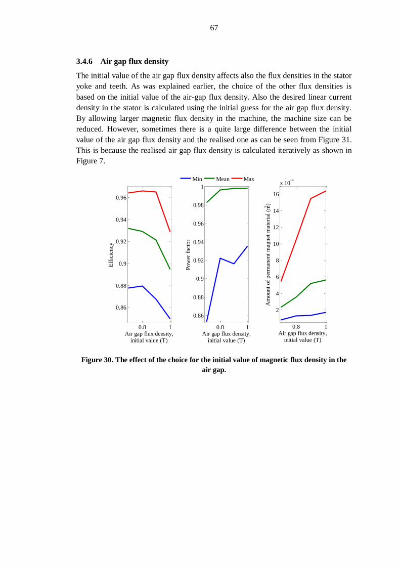
3.4.6 Air gap flux density .................................................................................... 67

4 Discussion ...................................................................................................... 70

4.1 Conclusions ....................................................................................................... 70

4.2 Further work ...................................................................................................... 73

References ............................................................................................................. 75

Appendix 1: Explanation of the d- and q-axis and the inductances ......................... 77

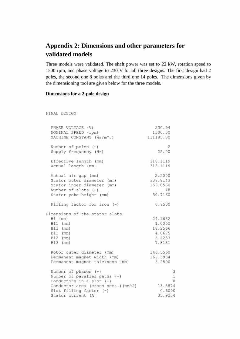
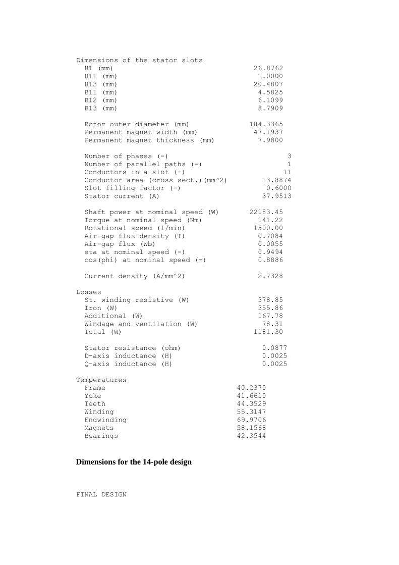
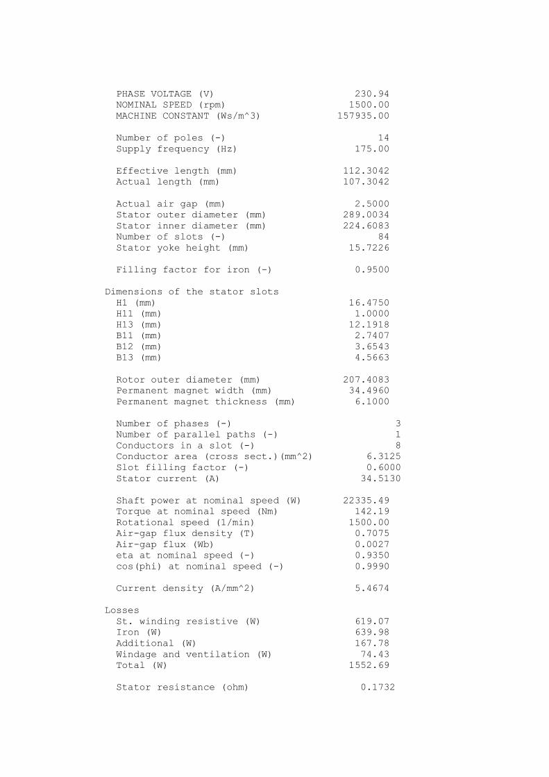
Appendix 2: Dimensions and other parameters for validated models ...................... 79

Nomenclature

Abbreviations

AC Alternating current

AlNiCo Aluminium-nickel-cobalt

DC Direct current

EMF Electromotive force

FEM Finite element method

NdFeB Neodymium-iron-boron

PMSM Permanent magnet synchronous machine

Symbols

Latin

armature linear current density

number of parallel paths

empirical heat transfer constants

peak magnetic flux density

width

machine constant related to apparent power

coefficient

power factor

diameter

back induced EMF

bearing load

frequency

iron space factor

thermal conductance

thermal conductance matrix

magnetic field strength

height

current

current density

empirical coefficients

number of parallel conductors in one slot

copper space factor

saturation factor

coefficient for iron losses, teeth

coefficient for iron losses, yoke

distribution factor

pitch factor

resistance factor

winding factor

length, thickness

effective machine length

inductance

average length of a coil turn

total length of a conductor in a coil

length of one coil turn

thickness of permanent magnets

effective thickness of permanent magnets

width of permanent magnets

mass, number of phases

number of turns in a winding

Nusselt number

number of coil turns in a slot

number of coil turns in a phase

rotating speed

synchronous speed

number of ventilation ducts

number of phases

output power

mechanical losses

resistive losses

iron losses

electrical power

mechanical power

additional losses

heat flow source vector

pole pair number

coefficient

number of slots

number of slots per pole per phase

resistance, reluctance, thermal resistance

radius

area [m2], apparent power

torque, temperature

Taylor number

modified Taylor number

relative torque

fundamental torque

time

stator phase voltage

velocity

coil span (width)

tooth width

number of conductors in a slot

Greek

relative magnet width

heat transfer coefficient

slot angle

coefficient

air-gap

load angle

relative emissivity

efficiency

temperature difference temperature vector

thermal conductivity [W/K m]

relative permeability of permanent magnets

permeability of vacuum, constant [V s/A m] ordinal of harmonic, magnetic voltage

kinematic viscosity of air

the ratio of the equivalent machine length to the air-gap diameter

constant, 3.14…

mass density

electrical conductivity

Stefan-Boltzmann constant, 5.67 *10-8

W/m2K

4

pole pitch

slot pitch

length of the pole pitch in the middle of the yoke

magnetic flux, heat flow rate

mechanical angular speed

angular frequency

Subscripts

0 shortest

1, 2, 3, … numbers, indexes

AC alternating current

Al aluminium

av average

b bearing

bb from bearing to bearing

c coil

cond subconductor

cr contact between the rotor yoke and the shaft

cy contact between yoke and frame

d d-axis

DC direct current

eff effective

es end shield

Fe iron

fin cooling fin

fr frame

i index

if internal frame

ins insulation

Ir insulation

m magnets

md magnetizing inductance, d-axis

mec mechanical

mq magnetizing inductance,q-axis

n nominal

p width of permanent magnets

ph phase

PM permanent magnets

q q-axis

r rotor

s slot, stator

se stator outer

sh shaft

sl retaining sleeve

sq skew

T temperature

th thermal

tt tooth tip

u slot

v ventilation duct

ve equivalent ventilation duct

w endwinding

wp working period

x,y per unit length

x0, y0 slot material, effective rectangular slot

y yoke

yr rotor yoke

z teeth

air-gap

leakage

11

1 Introduction

Permanent magnet synchronous machines (PMSMs) were first introduced in the

1930’s when the AlNiCo magnet material was discovered. However, at that time the

performance of the magnet material was not sufficient and variable frequency power

sources did not exist, which made the use of the PMSM very limited. Nowadays the

permanent magnet materials are better, particularly after the neodymium-iron-boron

(NdFeB) -magnets were discovered in 1983. It is also possible to use frequency

converters to control the PMSMs. These improvements have made permanent

magnet synchronous machines more popular. [1]

The permanent magnet synchronous machine has several advantages such as a

maintenance-free operation, high controllability, robustness against the environment,

high power factor and high efficiency. The environmental problems have caused a

need to save energy. This means a growing demand for highly efficient electrical

machines. The development of high performance magnet material in addition to

environmental issues has expanded the field of applications for PMSM. [1] The

PMSMs are widely used for example in hybrid vehicles.

In order to be able to produce efficient and compact PMSMs, the design criteria have

to be known. There are certain properties that are interesting from the energy

conservation point of view, for example efficiency, power density and power factor.

Also the material costs have to be taken into account. For example the permanent

magnet materials are usually rather expensive. Compared to the price of copper, the

price of NdFeB-magnet material is about 11 times higher [2], [3]. These properties

can be affected by changing several different design parameters. The parameters

include pole pair number, the size of permanent magnets, the type of winding, etc.

The design of an electrical machine is a rather complicated task that contains several

steps. During these steps, some of the qualities of the machine become fixed by

means of empirical equations. This makes the optimization of the machine design a

rather difficult task. In order to be able to define an optimal solution for certain

initial conditions, it is important to know how the different design parameters affect

the final outcome. For example the pole pair number might have a certain effect on

the size of the machine or the stator current density might affect the efficiency.

Because there are several parameters that have to be optimized, the final solution is

always a compromise between different criteria.

1.1 Objective

The objective of this Master’s Thesis is to investigate the effect of the design

parameters and find possible contradictions between different parameters. These

contradictions could then be used for optimization. One objective is to study how to

design more compact machines. To study the design parameters a dimensioning tool

12

is implemented using the MATLAB software of MathWorks [4]. The tool is based

on analytical design equations of electrical machines. The investigation is restricted

to surface mounted permanent magnet synchronous machines because of their simple

geometry. In addition, only single layer integer slot stator windings are considered at

this stage. Later it would be possible to further implement the dimensioning tool to

work also with for example other rotor or winding topologies.

The first chapter describes the structure and purpose of this thesis and introduces

permanent magnet synchronous machines. The second chapter discusses the design

process of PMSMs. Also the implemented design tool is presented. The analysis of

the effects of different design parameters is presented in Chapter 3 and the

conclusions drawn from this analysis are discussed in Chapter 4.

1.2 Permanent magnet synchronous machines

A synchronous machine is an electrical machine that operates at synchronous speed

meaning the speed at which the magnetic field rotates. The synchronous speed

depends on the frequency of the applied voltage and the number of poles in the

machine. The permanent magnet machines can be operated at unity power factor and

can therefore provide better efficiency than for example induction machines. The

PMSM has also high efficiency, high torque density and good heat dissipation. It is

possible to make the torque smooth and the pull-out torque high. On the other hand,

the PMSMs are expensive, because of the high prices of the magnet materials.

Because the magnetization is constant, the field weakening properties are poor

compared to ordinary synchronous machines. [5]

The basic components are stator and rotor. The stator is also the armature of the

synchronous machine. The stator core is made of thin laminations of highly

permeable steel. The stator core is placed inside an aluminium frame. The main

purpose of the frame is to provide mechanical support for the synchronous machine.

Inside the stator core there is a plurality of slots as can be seen from Figure 1. The

coils that form a polyphase winding, are arranged symmetrically in these slots. [6]

According to [6] the synchronous machines usually operate at three phase power and

the armature winding is thus made of three separate windings. The three phase

windings may be connected to either star (Y) or delta (Δ) connection. The winding

can be a single layer or a double layer winding. In a double layer winding there are

two coil sides in a slot whereas in a single layer winding there is only one. The

winding is an integer slot winding if the number of slots per pole per phase is an

integer. Otherwise the winding is called a fractional slot winding.

The armature winding of the synchronous machine produces a revolving magnetic

field. When the north pole of the field is just above the south pole of the rotor, the

force attraction between the two poles starts to move the rotor. Because the rotor is

13

heavy, it takes time before it can start moving, and by the time it starts to move, the

revolving field has changed its polarity. Now there are poles with alike polarity close

to each other and the repulsive force tries to move the rotor to the other direction.

This means that the synchronous machine is typically not self-starting without a

frequency converter. [6]

Figure 1. Structure of a two-pole surface-mounted permanent magnet synchronous

machine.

The rotor is rotated at synchronous speed. In permanent magnet synchronous

machines the main magnetic field is created by permanent magnets that are mounted

to the rotor. The rotor core is either solid iron, or made of laminations. The

permanent magnets can be mounted to the core in several ways. In surface

permanent magnet machines, the magnets are mounted on the surface of the outer

periphery of rotor laminations. Since the relative permeability of the magnet material

is close to one, this kind of structure has a large effective air gap, and the d-axis

inductance is thus low. [5] (See Appendix 1 for the definitions of the d- and q-axis.)

14

Because the permanent magnets produce a constant flux in the air gap, the field

weakening properties of a surface magnet machine are poor. Most of the current

would go to demagnetization, and very little current would be left to produce torque.

If high operation speed is needed, the nominal rotation speed of the surface mounted

PMSM should thus be close to the needed operation speed. The surface magnet

construction might also need a fibre glass band to make the construction

mechanically robust enough. One drawback is also that the frequency converter

produces higher order harmonics. An advantage of the surface magnet construction

is that the leakage flux is low, because there is no ferromagnetic path for the flux at

the edges of the magnet. Reduced quadrature axis inductance decreases the armature

reaction which leads into a smaller pole angle and higher torque. For this reason, less

permanent magnet material is usually needed for the surface magnet machine than

for the interior magnet machine. [5] High speed machines are typically surface

mounted PMSMs.

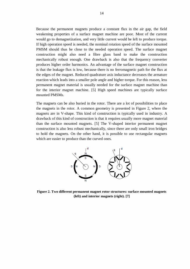
The magnets can be also buried in the rotor. There are a lot of possibilities to place

the magnets in the rotor. A common geometry is presented in Figure 2, where the

magnets are in V-shape. This kind of construction is typically used in industry. A

drawback of this kind of construction is that it requires usually more magnet material

than the surface mounted magnets. [5] The V-shaped interior permanent magnet

construction is also less robust mechanically, since there are only small iron bridges

to hold the magnets. On the other hand, it is possible to use rectangular magnets

which are easier to produce than the curved ones.

Figure 2. Two different permanent magnet rotor structures: surface mounted magnets

(left) and interior magnets (right). [7]

15

2 Methods

2.1 Design procedure

2.1.1 Initial parameters

Usually the electrical machine is designed for given initial conditions. The system

for which the machine is intended defines the requirements concerning shaft power,

supply voltage and speed.

Besides the above ones, there are several other initial parameters that also affect the

machine design process. The current density in the stator winding and the magnetic

flux density in the air-gap can be estimated relatively easily because there are certain

restrictions to both of them. If the magnetic flux density is too low, the iron core is

not utilized well. On the other hand when the flux density is too large, the iron will

saturate. If the current density is too high the conductors will overheat, which may

damage the insulations. According to [8] the current density in a stator winding of a

PMSM varies between 4-6.5 A/mm2 and the air gap flux density of a non-salient

pole synchronous machine varies between 0.8-1.05 T.

Initial estimates for efficiency and power factor are chosen. An initial value for the

needed electrical power is calculated using the estimated efficiency

(1)

where is the mechanical power. The linear current density is also estimated. In

order to find the linear current density, the machine constant has to be determined.

The machine constant expresses the magnitude of the internal apparent power or

mechanical power given by the rotor volume of the machine. Because the machine

constant can be calculated using either apparent power or mechanical power, it

means that there are actually two slightly different machine constants. Here the

mechanical machine constant is used to determine the mechanical dimensions

and the apparent machine constant is used to obtain the desired linear current

density in the stator.

There is a relation between the mechanical machine constant and the apparent

machine constant. According to [8] the apparent power is

(2)

where is the synchronous speed is the effective length of the machine and

is the air gap diameter i.e. stator inner diameter. The mechanical power is

16

(3)

where is the power factor and is the back induced electromotive force

(back-EMF). By substituting in Equation (3) with Equation (2), we get

(4)

Now a relation between the apparent and the mechanical machine constants is

obtained

(5)

where is the phase voltage. For rotating electrical machines the apparent

machine constant can be written also

√ (6)

where is the linear current density in the stator, is the peak flux density in the

air gap and is a winding factor which depends on the winding arrangement.

Here Equation (5) is used to solve the initial value of the linear current density. At

this point of the design process, the actual value of the winding factor is not yet

known, but since it does not vary very much, it can be guessed to be for example

0.92 just to obtain an initial guess for the linear current density.

The pole pair number depends on the speed and the frequency

(7)

If the machine is supplied from a frequency converter, which normally is the case

with PMSMs, the machine properties can be affected by choosing a suitable number

of poles.

2.1.2 Mechanical dimensions

The most interesting mechanical dimensions are the actual length of the machine and

the stator outer diameter, because these two roughly determine the machine size. The

larger these values are the larger the machine volume and usually the heavier the

mass usually are. To be able to construct the mechanical parts of the machine, also

the detailed dimensions for the stator and rotor are needed.

17

In the case of the stator, the inner and outer diameters of the stator core, the height of

the yoke and the teeth, the width of the teeth, the slot dimensions and the number of

slots need to be found. The slot dimensions depend on the chosen slot shape. The

rotor dimensions in this case are the rotor inner and outer diameter.

There are two mechanical dimensions that are considered as free design parameters,

namely air gap length and ratio of machine length to stator inner diameter. Pyrhönen

et. al. [8] give also equations to get typical values of these parameters.

The ratio of the effective machine length to the air-gap diameter is

(8)

where is the effective machine length and is the air-gap diameter.

For synchronous machines this value is typically [8]

√ (9)

(10)

The mechanical machine constant can be obtained from a figure given by [8] p.

289, when is known. The mechanical power is

(11)

Now it is possible to solve the air-gap diameter from Equation (11)

√

(12)

and the effective length from Equation (8).

The stator dimensions can be defined when the machine constant is known. These

are stator length, the inner and outer diameters of the stator and number of slots in

the stator and the length of the air-gap.

The air-gap of a synchronous machine can be estimated by equation

(13)

where is a coefficient. For example Pyrhönen et. al. [8] provide a table for

choosing a suitable value for . is the armature linear current density, is the

18

peak air-gap flux density and is the pole pitch. In PMSMs the air-gap length is

determined by mechanical constraints. It is similar to the values encountered with

asynchronous machines, and can therefore be calculated using same equations [8]:

(14)

(15)

Now also the rotor core diameter can be calculated from equation

(16)

where is the air gap and is the thickness of the permanent magnets.

The effective machine length differs from the real machine length for two reasons.

First, there are ventilation ducts in the machine that make the machine real length

larger than the effective. The effect of the air-gap has to be taken into account too.

The effective length of the machine is

(17)

which means that the actual length is approximately

(18)

where is number of ventilation ducts and is the effective width of the

ventilation ducts.

2.1.3 Winding

The next task is to design a suitable winding for the machine. Only single layer,

integer slot windings are considered here. There is only one coil side in each slot and

the number of slots per pole per phase is an integer. The two main tasks of the

design procedure are to define a suitable winding and to find suitable dimensions for

the permanent magnets. These two properties are connected to each other via the

back induced EMF

√ (19)

It can be seen from Equation (19) that the back-EMF depends on the number of coil

turns in a phase , the maximum magnetic flux in the air-gap , the winding

factor and the supply frequency . The winding factor and the number of coil

19

turns in a phase depend on the winding whereas the air-gap flux is generated by the

permanent magnets. The back-EMF affects the power factor of the machine. If the

back-EMF is close to the phase voltage, the power factor should be close to one.

This means that when the winding is defined, the permanent magnet dimensions can

be solved using Equation (19). Designing the winding includes defining the number

of slots per pole per phase, number of conductors in a slot and number of coil turns

in a phase. The winding is chosen so that the obtained linear current density is close

to the approximated one. The linear current density depends of the number of coil

turns and the stator inner diameter

(20)

where is the stator current and is the number of phases. When the winding is

chosen, the winding factor is calculated. The winding factor of a harmonic is

(21)

where the pitch factor is

(

) (22)

and the distribution factor is

(

)

(

) (23)

where

(24)

is the slot pitch angle which is measured in electrical degrees, is the number of

slots per pole per phase, and is the number of slots. can be ,

where is any positive integer or zero and is the number of phases. For one layer

winding, , which makes the pitch factor

(

) (25)

The number of the stator slots defines the slot pitch

(26)

20

The maximum number of slots is reduced by the length of the stator inner periphery.

Typical slot pitches are given in [8]. For small PMSMs this is 7-45 mm and for large

PMSMs 14-75 mm. The number of stator slots can also be determined by defining

the number of slots per pole per phase

(27)

2.1.4 Permanent magnets

Next, the permanent magnets will be designed. The material of the magnets is

chosen and the dimensions are defined. The most important characteristics for the

permanent magnet material are the remanence flux density , coercive field strength

, the second quarter of the hysteresis loop, the energy product, temperature

coefficients of the remanence flux density and coercive field strength, resistivity, and

mechanical and chemical characteristics. [8]

Two common permanent magnet rotor structures are a surface permanent magnet

rotor and an interior permanent magnet rotor, where the magnets are in a V-shape.

These structures are presented in Figure 2. Since the geometry and calculations are

simpler with surface magnets than with interior magnets, the surface magnet rotor

was chosen for this study.

The surface magnet dimensions include the thickness of the permanent magnets

and the width of the magnets . The width has to be smaller than the pole pitch

. Usually the magnet width is about 0.8 – 0.85 times the pole pitch. [9] The

magnet thickness should be as small as possible to keep the amount of permanent

magnet material that is needed low. However, the magnets have to be thick enough

to produce the required air-gap magnetic flux. The magnet thickness can be chosen

iteratively when a suitable width has been chosen. The thickness is optimal when the

back-EMF calculated by Equation (19) equals approximately the phase voltage. It is

possible to allow the back-EMF to be smaller than the phase voltage, but that will

also lead to a smaller power factor.

2.1.5 Calculating the flux and the flux density

Now the magnetic flux and flux density in the air-gap are calculated. For this

purpose, a reluctance network model of the machine is employed. In Figure 3 a

reluctance network for a surface magnet PMSM is presented. is the reluctance

of the permanent magnets, is the iron reluctance which consists of the stator

teeth reluctance and the stator yoke reluctance . is the reluctance of the air-

gap between two magnets and is the air-gap reluctance in the minimum air-gap

between the stator and the magnets. is the total magnetic flux of the permanent

magnets, is the air-gap flux and is th–e leakage flux. [7]

21

Figure 3. Reluctance network model for a surface magnet PMSM.

The equation for the air-gap flux can be derived from the reluctance network

( )

( ( ))

(28)

The reluctance of the air-gap between the permanent magnets and the stator is

(29)

The reluctance of the air-gap between two magnets is

( ) (30)

The reluctance of the permanent magnets is

(31)

where is the thickness of the insulation layer between the rotor and the magnets,

is the thickness of the magnets and is the magnet width, is the actual length of

the machine, is the permeability of vacuum and is the relative permeability

of the permanent magnets.

Calculation of the magnetic flux is an iterative process. Because the slot dimensions

are not known beforehand, it is not possible at the first iteration to calculate the iron

reluctance. This problem is solved by calculating an initial guess for the magnetic

flux density in the air-gap. This is used to solve the magnetic flux from Equation

22

(32). Now it is possible to solve the slot dimensions. This is explained more

carefully in Section 2.1.6.

The maximal air-gap flux density is

( ) ( )

(32)

where is the relative magnet width

, is the pole pitch, and is the

effective length of the machine. [7]

If the slot dimensions are known, the iron reluctance is relatively simple to calculate.

The yoke reluctance is

(33)

where is the yoke width, is the yoke height and is the permeability of iron

in the yoke. The reluctance of the teeth is

(34)

where is the tooth height, the tooth width and the permeability of iron in

the tooth. The total iron reluctance is now

(35)

2.1.6 Slot dimensions

When the magnet dimensions and the air-gap flux density are known, the next step is

to calculate the dimensions of the stator slots and teeth. Here, the tooth width is

chosen to be constant and the slot shape is presented in Figure 4. The needed slot

dimensions are the minimum width bs1, maximum width bs2, height and the

height of the conductor area h4. The height is used for both slot and tooth heights.

23

Figure 4. Stator slot shape.

At first step, the maximum magnetic flux densities for the teeth and the yoke are

selected. According to [8] a maximum value for the tooth flux density is 1.5-2.0 T

and for the yoke 1.1 – 1.5 T. Because the air-gap flux density distribution is

rectangular in the air gap, the flux density in the teeth is

(36)

above the magnets and zero elsewhere. [7] denotes the cross-sectional area of a

tooth and according to [8] it is

( ) (37)

where is the filling factor for the iron laminates, is the number of ventilating

ducts and is the width of the a duct. The maximum magnetic flux passing through

one slot pitch is

(38)

When the tooth is not saturated almost all the flux goes through the tooth, which

means that the flux density in the tooth is

24

( ) (39)

where and is the space factor of laminated iron. Typically

varies between 0.9 and 0.97. The tooth width can be solved from Equation (39)

when the maximal value of the magnetic flux density in a tooth is defined. The slot

width is

(40)

where is the stator slot pitch.

The length of the stator slot can be determined when the slot area and width are

known. In order to calculate the slot area the stator current has to be defined

first

(41)

Now the area of conductors is

(42)

and the slot area is

(43)

in which is the current density in the conductors. It is a design parameter that has

to be chosen in the beginning of machine design. Furthermore, the denotes the

number of conductors in a slot, the area of a conductor and the space factor of

a slot. The space factor depends of the winding material, the voltage level and

the winding type. For low-voltage machines, typical values are ( ) and

for high-voltage machines ( ), the lower value being for round wires

and the upper value for rectangular wires. The number of conductors in a slot is

defined as

(44)

When the slot area and the minimum slot width are known, the other dimensions can

be calculated.

is the total area of the slot. The area that is left between the tooth tips is not taken

into account, because there are no conductors in that area. The slot area can be

25

divided into two parts: a half circle and a trapezium. Now the equation for the area is

obtained from geometry

( )

(

)

(45)

where is the height of the trapezium and the other dimensions are as presented in

Figure 4. On the other hand the pole pitch reduced to the widest point of the slot is

( )

(46)

Now there are two equations, (45) and (46), from which the two unknown

parameters, maximum slot width and trapezium height , can be solved. The

slot opening is assumed to be 3/4 of the minimum slot width and heights

and are both 1 mm. The slot height satisfies

(47)

where height is given as

(48)

To define the yoke height , the maximum magnetic flux in the stator yoke has to

be calculated. This is rather easy, since in the yoke the maximum flux, namely half

of the main flux, flows on the quadrature axis.

( )

( )

(49)

By choosing a maximum allowed value for the flux density in the yoke, the yoke

height can now be obtained. The stator outer diameter is

(50)

2.1.7 Inductances

When the winding arrangement and the dimensions have been defined, the

inductances can be calculated. According to [7] the magnetizing inductance of the

direct axis is

( )

(51)

26

where is the effective length of the air-gap that depends on the real air-gap

length , the thickness of the permanent magnets and the effect of the saturated

iron. In PMSMs, the effective air-gap is obtained as [8]

(52)

The magnetization inductance of the quadrature axis is similar to the d-axis

magnetisation inductance, and the effective air gap can be calculated using

Equation (52).

( )

(53)

The synchronous inductances and consist of the magnetizing inductances and

leakage inductances

(54)

(55)

For more information about the inductances, see Appendix 1. The leakage

inductances are assumed to be equal for direct and quadrature axis. The leakage

inductance consists of air-gap leakage inductance , slot leakage inductance ,

tooth tip leakage inductance , end winding leakage inductance and skew

leakage inductance .

(56)

The air-gap leakage inductance can be calculated multiplying the magnetizing

inductance by a leakage factor

(57)

∑ (

)

(58)

To calculate the slot leakage inductance accurately the slot type and the detailed

dimensions have to be known. The slot shape chosen for this study is shown in

Figure 4. The slot leakage inductance is

(59)

where

27

(60)

Parameters and are heights and widths of different slot parts as presented in

Figure 4.

The tooth tip leakage inductance for the whole phase winding is obtained by

substituting instead of in Equation (59).

(61)

(

)

(

) (62)

The coefficient , when

.

The end winding inductance is

(63)

where is the average length of the end winding and the product

can be written in the form

(64)

in which is the axial length of the end winding measured from the end of the

stack, is the coil span and and are the corresponding permeance factors

[8].

2.1.8 Torque, resistances and power losses

The torque of the machine consists of the fundamental torque and the reluctance

torque : . According to [7] they can be calculated by equations

(65)

(

) (66)

28

From Equation (66) it can be seen that when the machine is non-salient, i.e. ,

the reluctance torque and the torque becomes . This is the case with

surface magnet machines.

The resistance can be calculated using equations presented in [8]. The DC resistance

is

(67)

where is the length of a conductor in a coil, is the conductivity of the conductor

material and is the cross sectional area of the conductor. The AC resistance is

(68)

where is a resistance factor that takes into account skin effect in the conductors.

is the average length of a coil turn. For low voltage machines with enamelled

wires it is approximately

(69)

where is the average coil span. For large machines with prefabricated wires the

average turn length is

(70)

or

(71)

when . The length of a conductor in a coil can be approximated

. The resistance factor kR depends on the reduced conductor height that

satisfies

√

(72)

where and are the height and width of a sub-conductor, respectively. If the

reduced conductor height is , a good approximation for the resistance

factor of rectangular wires is

(73)

The electrical power is

29

(

) (74)

When the electrical power is known, the load angle can be solved from Equation

(74). The problem here is that the efficiency cannot be known beforehand, which

means that the electrical power is in fact not known. It is possible to use the chosen

initial guess of the efficiency to estimate the electrical power, but this is not a very

accurate method.

Therefore another method was chosen. The electrical power of a motor is

(75)

This means that if the losses can be calculated or approximated, the electrical power

can be evaluated using the desired shaft power. By looking at Equations (81)-(85), it

can be seen that all other losses except copper losses can be calculated at thi–s point.

In order to find the copper losses the stator current has to be known. The stator

current can be calculated from its d- and q-axis components, which depend on the

inductances, resistance, phase voltage, back-EMF, frequency and load angle, as can

be seen from Equation (76) and (77). All of these parameters are known except the

load angle, which means that the current can be considered as a function of the load

angle.

Now there are two possible ways to obtain the electrical power: Equation (75) and

Equation (74). Combining these two equations results in an equation from which the

load angle , can be solved.

A method to calculate the currents and is presented by Jussila [9] for non-

salient pole machines.

( )

(76)

( )

(77)

The stator current is

√

(78)

The maximal current density is

30

(79)

and the linear current density is

(80)

where is the stator inner radius. The losses consist of resistive losses in stator

conductors, iron losses in the magnetic circuit, mechanical losses in the bearings, and

additional losses. The resistive losses are

(81)

The iron losses are

(

)

(

)

(82)

where and are the mass of the yoke and the teeth, and are

empirical correction coefficients and is a coefficient depending of the material.

The mechanical losses consist of the windage and ventilation losses and the

bearing losses .

( ) (

)

(83)

(84)

where is the angular velocity of the shaft supported by bearing, is the friction

coefficient (typically 0.001-0.005), the bearing load and the inner diameter of

the bearing.[8]

The additional losses are very difficult to calculate or measure. One assumption is

(85)

where is the nominal output power. For a motor, the output power is the shaft

power . When the losses are known, the efficiency can be calculated

(86)

31

2.1.9 Heat transfer

Finally, the heat transfer has to be modelled in order to make sure that the machine is

not overheated. Figure 5 shows the heat flow in a surface mounted PMSM. The

modelling is done by using a thermal network presented in Figure 6.

There are three different methods of heat transfer: conduction, radiation and

convection. Conduction is heat transfer either by molecular interaction or between

free electrons. It is possible between solids, liquids and gases.

The thermal network consists of thermal resistances . Analogous to electrical

resistances, they are defined as the ratio of the potential difference to the current, i.e.

ratio of temperature difference to the heat flow rate . The thermal resistance for

conduction can be calculated

(87)

where is the length of the conductor, is the conducting area and is the thermal

conductivity of the conductor.

The second form of heat transfer is radiation. It means electromagnetic radiation

which has its wave length between 0.1 and 100 µm. Unlike the other two heat

transfer methods, radiation does not need a medium for heat exchange. The thermal

resistance of radiation is analogous to that of conduction

(

) (88)

where is the relative emissivity between the emitting and absorbing surfaces,

the Stefan-Boltzmann constant, the thermodynamic temperature of the

radiating surface and the thermodynamic temperature of the absorbing surface.

The third type of heat transfer is convection. It means heat transfer between a region

of higher temperature and a region of cooler temperature via a moving fluid. Heat is

always transferred simultaneously by conduction and convection. The thermal

resistance of convection satisfies

(89)

where is the heat transfer coefficient that depends on the viscosity of the coolant,

the thermal conductivity, specific heat capacity and the flow of the medium.

Traditionally it has been defined by empirical relations. According to [8] the heat

transfer coefficient for natural convection in the air around a horizontally mounted,

32

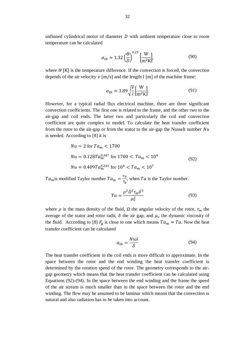
unfinned cylindrical motor of diameter with ambient temperature close to room

temperature can be calculated

(

)

[

] (90)

where is the temperature difference. If the convection is forced, the convection

depends of the air velocity and the length of the machine frame:

√

[

] (91)

However, for a typical radial flux electrical machine, there are three significant

convection coefficients. The first one is related to the frame, and the other two to the

air-gap and coil ends. The latter two and particularly the coil end convection

coefficient are quite complex to model. To calculate the heat transfer coefficient

from the rotor to the air-gap or from the stator to the air-gap the Nusselt number

is needed. According to [8] it is

for

for

for

(92)

is modified Taylor number

, when is the Taylor number.

(93)

where is the mass density of the fluid, the angular velocity of the rotor, the

average of the stator and rotor radii, the air gap, and the dynamic viscosity of

the fluid. According to [8] is close to one which means . Now the heat

transfer coefficient can be calculated

(94)

The heat transfer coefficient in the coil ends is more difficult to approximate. In the

space between the rotor and the end winding the heat transfer coefficient is

determined by the rotation speed of the rotor. The geometry corresponds to the air-

gap geometry which means that the heat transfer coefficient can be calculated using

Equations (92)-(94). In the space between the end winding and the frame the speed

of the air stream is much smaller than in the space between the rotor and the end

winding. The flow may be assumed to be laminar which means that the convection is

natural and also radiation has to be taken into account.

33

The thermal network consists of thermal resistances that are analogous to electrical

resistances. Resistive losses, iron losses, windage losses and friction losses are

represented by individual heat flow sources. The heat capacity is analogous to

electric capacitance. Figure 5 represents the different types of heat transfer in a

permanent magnet synchronous machine. Convection is presented with green

arrows, radiation with purple arrows and conduction with red arrows. The radiation

inside the machine is not taken into account in the figure.

Figure 5. The heat transfer in a rotor surface mounted permanent magnet synchronous

machine. [10]

34

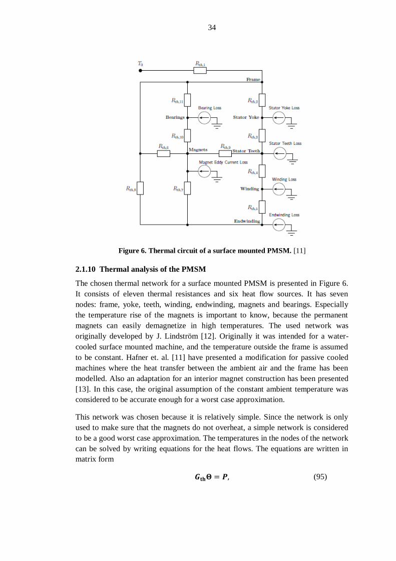
Figure 6. Thermal circuit of a surface mounted PMSM. [11]

2.1.10 Thermal analysis of the PMSM

The chosen thermal network for a surface mounted PMSM is presented in Figure 6.

It consists of eleven thermal resistances and six heat flow sources. It has seven

nodes: frame, yoke, teeth, winding, endwinding, magnets and bearings. Especially

the temperature rise of the magnets is important to know, because the permanent

magnets can easily demagnetize in high temperatures. The used network was

originally developed by J. Lindström [12]. Originally it was intended for a water-

cooled surface mounted machine, and the temperature outside the frame is assumed

to be constant. Hafner et. al. [11] have presented a modification for passive cooled

machines where the heat transfer between the ambient air and the frame has been

modelled. Also an adaptation for an interior magnet construction has been presented

[13]. In this case, the original assumption of the constant ambient temperature was

considered to be accurate enough for a worst case approximation.

This network was chosen because it is relatively simple. Since the network is only

used to make sure that the magnets do not overheat, a simple network is considered

to be a good worst case approximation. The temperatures in the nodes of the network

can be solved by writing equations for the heat flows. The equations are written in

matrix form

(95)

35

where is the thermal conductance matrix of the network, is the temperature

vector and is the heat flow source vector. The temperatures can be solved from

Equation (95)

(96)

[

]

(97)

in which

(98)

(99)

(100)

(101)

(102)

(103)

(104)

and are the individual thermal conductances of the network

.

The thermal resistance of the network consist of the thermal resistances of the

different machine parts.

(105)

( ) (106)

( ) (107)

( )(

( )) (108)

36

(109)

(110)

(111)

(112)

(113)

(114)

(115)

Next the methods to calculate the thermal resistances of the different machine parts

are explained. The stator has four thermal resistances: frame, yoke, teeth and the

contact resistance between the frame and the yoke. The resistance of the frame is

( ) (116)

where is the height of the frame and is thermal conductivity aluminium,

which is for electro-technical aluminium [8]. The yoke thermal

resistance is

(

)

(117)

where is the thermal conductivity of iron (74.7 W/ m·K). The contact between

the stator yoke and frame has also its own thermal resistance because of the contact

of two different materials. According to [12] this contact resistance equals to

equivalent gap divided by thermal conductivity and area of the gap. These

parameters are rather difficult to obtain so the contact resistance is assumed to be

equal to the thermal resistance of the yoke. The thermal resistance for the teeth is

according to [12] an integral

37

∫

( )

(118)

where ( ) is the tooth length at height . In this case the tooth length is equal

everywhere except at the tooth tip. This is considered to be a minor deflection of the

tooth width, and the tooth is assumed to have equal width everywhere. This means

that the resistance becomes

(119)

Equation (119) gives a single resistance for all the stator teeth. Next the thermal

resistances from internal air to the frame , rotor and end winding are

calculated.

(120)

where is empirically defined heat transfer coefficient

(121)

and is the area exposed to convection.

(122)

is the internal end shield area and is the internal frame area. These can be

calculated from machine dimensions. is the thermal resistance between the rotor

and the internal air.

(123)

where is an experimental coefficient

( ) (124)

and is again the area exposed to convection. According to [12], it can be

calculated

(125)

where is the air-gap radius and and are the width, height and number

of the cooling fins of the rotor. If the rotor is unfinned, it means that .

Resistance is the thermal resistance between the end winding and the internal air.

38

(126)

is the area of the end winding and is an empirical heat transfer coefficient.

( )

(127)

Because the temperature of the internal air of the motor is not required as a result,

the thermal network can be simplified by making a wye-delta transform for

resistances and . Thermal resistances and are transformed

from and .

is the thermal resistance of the air-gap. It can be calculated using equation

(128)

where is the heat transfer coefficient for the air-gap.

(129)

is the Nusselt number

( )

( ) (130)

and ( ) is the modified Taylor number. [12]

( )

(131)

in which is the kinematic viscosity of air. It is temperature dependent which

means that the temperature in the air-gap has to be estimated. If the modified Taylor

number becomes smaller than 1740, the airflow is considered to be without Taylor

vortices, and the Nusselt number is then 2.

The thermal resistance of the permanent magnets is

(

) (

)

(132)

where is the thermal conductivity of the permanent magnet material. is

the thermal resistance of the insulation between the magnets and the rotor yoke.

39

(133)

where is the thickness of the insulation layer and is the thermal conductivity

of the insulation material. The thermal resistance of the rotor yoke is

( ) (

)

(134)

The contact resistance between the rotor core and the shaft is assumed to be

equal to that of the rotor core.

It is assumed that the heat flow in the shaft goes to the axial direction. The thermal

resistance of the shaft is

(

)

(135)

where is the thermal conductivity of the shaft and is the distance between the

two bearings. is the thermal resistance of one bearing

( )( ) (136)

where are empirical coefficients. According to [14] they are valid only if

and

.

40

Table 1. Explanation for the different thermal resistances.

Symbol Thermal resistance

Frame

Stator yoke

Contact resistance between the yoke and the frame

Teeth

Per unit length resistances for Equation (108).

Slot material resistances (equivalent rectangular slot)

Winding

Between frame and internal air

Between rotor and internal air

Between end winding and internal air

Air-gap

Retaining sleeve

Permanent magnets

Insulation between magnets and rotor yoke

Rotor yoke

Contact between the rotor core and the shaft

Shaft, axial

One bearing

2.2 MATLAB implementation

A dimensioning tool for surface mounted permanent magnet synchronous machines

was implemented using the MATLAB software. The flow chart of the program is

presented in Figure 7.

The initial parameters are chosen during steps 1-4. These parameters are quite free to

choose. At step 5 the machine constant that depends on the pole power is defined.

The program does it automatically according to a figure presented on page 289 in

[8], but it is also possible to make the choice manually. At step 6 some of the main

mechanical dimensions are defined. These are machine length, stator inner diameter

and the effective machine length. The apparent machine constant and initial values

for stator current and linear current density are calculated during step 7 using

Equations (5) and (6).

At step 8 a suitable winding is chosen based on the estimated linear current density

value. The winding is a single layer winding. The magnet material, magnet width

and a guess for the magnet thickness are chosen during step 9.

At step 10 a new value for magnetic flux density is calculated using Equation

(6).The dimensions of the stator slots are calculated during steps 11-13. At steps 14

and 15, new values for the air gap flux and flux density are defined by calculating

41

the iron reluctance. Steps 11-15 are repeated until the air gap flux does not change

more than 0.001 T. At step 17 the back induced EMF is calculated using Equation

(19). If the back-EMF is close to the phase voltage, the magnets are thick enough.

Otherwise steps 10-17 have to be recalculated with thicker magnets. The rest of the

machine properties are calculated during steps 19-23 as presented in Section 2.1.8

The thermal network is also implemented with MATLAB. It follows the equations

presented in Section 2.1.10.

42

43

Figure 7. The flowchart of the dimensioning tool.

44

2.3 Operation profile

The design tool finds a solution for given input parameters. These parameters are

typically those for the rated operating point. Usually electrical machines are operated

at other conditions as well. This means that the machine has to have good

characteristics also for example, at lower rotation speeds than the rated speed. The

surface magnet machines are not usually used in rotation speeds higher than the rated

one, because that would require field weakening. With permanent magnets mounted

to the rotor surface, the air gap flux is constant, because it is produced by the

magnets. This makes the surface mounted PMSM quite poor in field weakening.

To ensure that the design that is obtained is truly feasible, it should be tested in other

operation points as well. Therefore, a method to calculate an operational profile for a

design is implemented. The method enables the calculation of the load angle, stator

current, electrical power, efficiency and power factor in different operation points.

If the operation point changes, it means that the rotation speed, voltage, power,

torque, back-EMF and frequency change. The relation between the torque and the

mechanical power is . It is assumed that the voltage is proportional to the

rotation speed. The back-induced EMF depends on the number of coil turns in a

phase, magnetic flux in the air gap and frequency. In a permanent magnet machine,

the air gap flux is constant because it is produced by the permanent magnets. This

means that the only changing parameter is the frequency.

All other parameters can be calculated if the load angle is known. The losses

depend on the machine parameters and rotation speed. In the chosen operating point,

they can be approximated because the machine parameters are known. When the

load angle is defined, it is possible to solve the stator current, efficiency, power

factor and electrical power in the operating point.

The interesting results from the analysis are the efficiency and power factor at

different rotation loadings. If the machine is operating at lower rotation speeds than

the rated speed, the efficiency might be worse than the nominal efficiency. By

studying the operation profile, information about the overall feasibility of the design

can be obtained.

The chosen operation profile is presented in Figure 8. The application is a 22 kW

industrial pump. The shaft power in different operation points is presented as a

function of rotation speed. The nominal voltage of the machine is 400 V. The

percentages for the operation points are presented in Table 2. Using these it is

possible to calculate a weighted average of the efficiencies and power factors. The

average efficiency and power factor over the whole working period are obtained

45

∑

(137)

∑

(138)

where is the efficiency of the operation point , is the time the machine is

working at operation point during the working period, and is the time of the

working period.

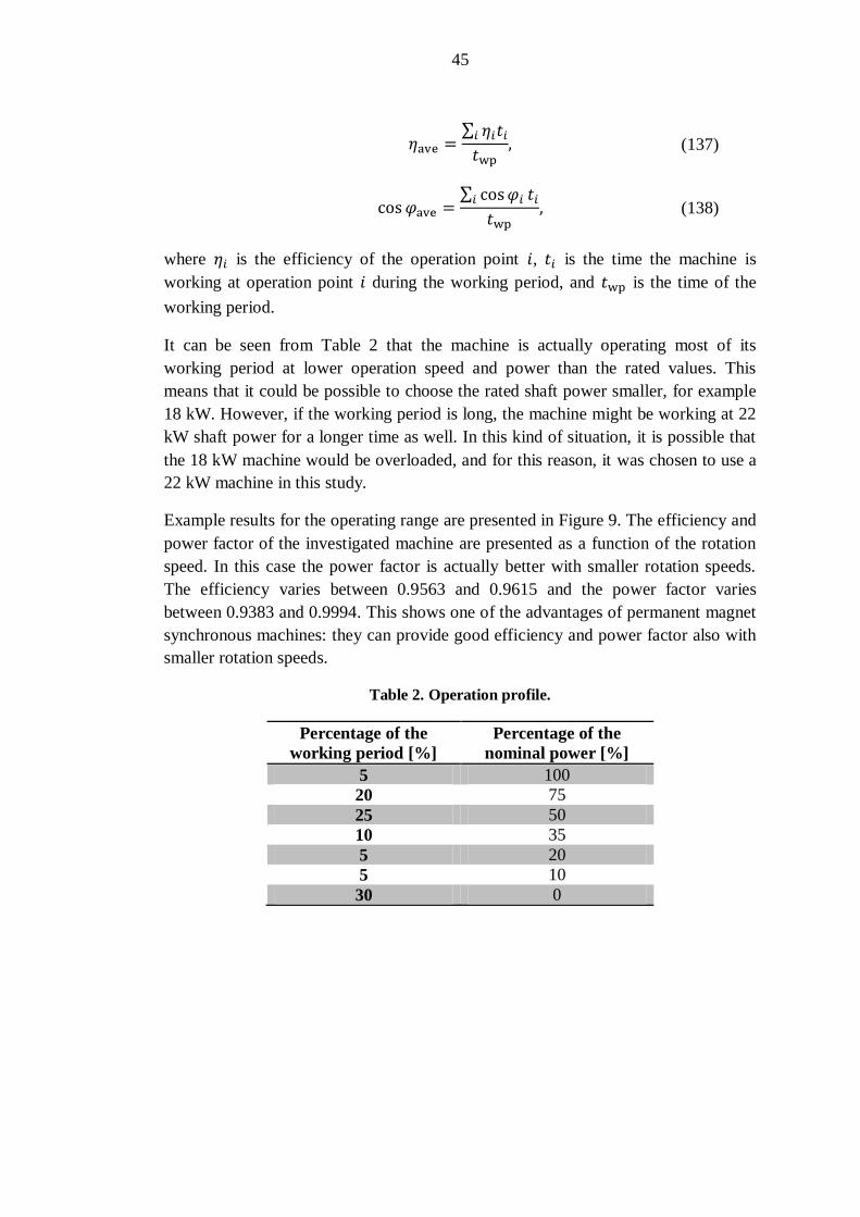
It can be seen from Table 2 that the machine is actually operating most of its

working period at lower operation speed and power than the rated values. This

means that it could be possible to choose the rated shaft power smaller, for example

18 kW. However, if the working period is long, the machine might be working at 22

kW shaft power for a longer time as well. In this kind of situation, it is possible that

the 18 kW machine would be overloaded, and for this reason, it was chosen to use a

22 kW machine in this study.

Example results for the operating range are presented in Figure 9. The efficiency and

power factor of the investigated machine are presented as a function of the rotation

speed. In this case the power factor is actually better with smaller rotation speeds.

The efficiency varies between 0.9563 and 0.9615 and the power factor varies

between 0.9383 and 0.9994. This shows one of the advantages of permanent magnet

synchronous machines: they can provide good efficiency and power factor also with

smaller rotation speeds.

Table 2. Operation profile.

Percentage of the

working period [%]

Percentage of the

nominal power [%]

5 100

20 75

25 50

10 35

5 20

5 10

30 0

46

Figure 8. The shaft power versus the rotation speed of the industrial pump that was

chosen for the application.

Figure 9. Example results for the operating range.

0

5

10

15

20

25

0 250 500 750 1000 1250 1500

Sh

aft

po

wer

(k

W)

Speed (rpm)

0 500 1000 15000.93

0.94

0.95

0.96

0.97

0.98

0.99

1

Rotation speed (1/min)

Pow

er f

acto

r

0 500 1000 15000.956

0.957

0.958

0.959

0.96

0.961

0.962

0.963

Rotation speed (1/min)

Eff

icie

ncy

47

3 Results

3.1 Validation of the dimensioning tool

After completing the dimensioning tool, the results had to be validated for ensuring

that the tool is working correctly. To be able to make conclusions, it is essential that

the results calculated with the dimensioning tool can be trusted.

The validation method was to first do the dimensioning with the implemented tool

and then verify the result using finite element method (FEM). The Flux2D software

of CEDRAT [15] was used for the FEM modelling and calculation. This way it is

possible to study more accurately how the obtained solution behaves. The results

calculated with FEM are compared with the ones obtained using the dimensioning

tool. This is done with three different machine constructions. The results should be at

least close to those obtained by the dimensioning tool. Some small differences might

appear since the dimensioning tool is based only on analytical equations which

include a lot of approximations. With FEM some of the machine properties, for

example magnetic flux densities and losses can be modelled more accurately.

Therefore it is enough if the results are close to each other.

The FEM results were calculated by Janne Keränen [16]. Three different designs

were tested: one with two poles, one with eight poles and one with 14 poles. The

dimensions and other parameters for the models are presented in Appendix 2. The

validation results are shown in Table 3, Table 4 and Table 5 for the 2-pole, 8-pole

and 14-pole designs, respectively.

For the 2-pole machine it can be seen that the FEM results and the dimensioning tool

results seem to be rather close to each other. The shaft power and torque agree well

with the analytically obtained values: the difference is less than 1 % of the

dimensioning tool results. Also the phase voltage and current of the FEM

calculations agree well with the analytical results. The back-EMF is also somewhat

close to the original value. However, it seems that the larger the pole pair number is

the smaller back-EMF the FEM calculations give. It was also observed that if there

are very many poles, the leakage flux from a magnet to its neighbouring magnet

becomes larger. This is not taken into account by the dimensioning tool, and can

therefore be one explanation to the difference in the back-EMF.

For 2- and 8-pole machines, efficiency and power factor are slightly smaller when

calculated with the dimensioning tool than with Flux2D. In the case of the

efficiency, some difference occurs because the Flux2D does not take into account the

core losses when calculating the efficiency. Therefore Flux2D can give larger

48

efficiency than the dimensioning tool. For the 14-pole design, the power factor is

larger when calculated with the dimensioning tool than the one obtained with FEM.

When comparing the power factors it must be taken into account that the

dimensioning tool assumes that the supply voltage is sinusoidal. This means that the

harmonics created by for instance a frequency converter are not taken into account.

In Flux2D, this kind of assumption has not been made which may cause a difference

between the power factors.

The losses seem to be slightly different when calculated with Flux2D than what the

dimensioning tool gives. For the two-pole design, the difference is 14 % in the

copper losses and 21 % in the iron losses. For the 8-pole design the results agree well

with each other: the differences are 0.3 % for the copper losses and 2.0 % for the

iron losses. For the 14-pole design, the difference between the copper losses

calculated with Flux2D and with the dimensioning tool is less than 1 %. On the other

hand, the iron losses obtained with Flux2D are half of the iron losses given by the

dimensioning tool.

One explanation for the differences in the iron losses is that the calculation method is

quite different. The dimensioning tool uses Equation (82) for calculating the iron

losses. The equation gives an approximation for total iron losses, including both

hysteresis and eddy current losses. The accurate calculation of the iron losses is in

any case rather difficult and requires modelling the physical phenomena in the iron.

Therefore also the iron losses obtained with Flux2D are also an approximation,

although possibly somewhat more accurate.

Table 3. Validation results for the 2-pole design.

Parameter Flux2D Dimensioning

tool

Back-EMF voltage [V] 240.1 230.9

Torque [Nm] 139.5 140.5

Stator current [A] 33.3 35.9

Phase voltage [V] 232.0 230.9

Electric power [kW] 22.6 23.2

Mechanical power [kW] 21.9 22.0

Efficiency rate 0.970 0.947

Power factor 0.976 0.936

Ohmic losses [W] 420.3 489.6

Core losses [W] 211.9 174.9

Back-EMF air-gap flux [Wb] 0.0354 -

Nominal point air-gap flux

[Wb] 0.0273 0.0339

49

Table 4. Validation results for the 8-pole model.


tool


Torque [Nm] 141.0 141.2











[Wb]

0.0565 0.0055

Table 5. Validation results for the 14-pole machine.


tool


Torque [Nm] 142.3 142.2











[Wb]

0.0026 0.0027

Also the thermal network is validated using the Flux2D. The thermal modelling can

be done much more precisely with the software, but since the thermal network used

by the dimensioning tool is quite simple, it was decided that a simple analysis would

be sufficient also with Flux2D. The temperatures of the different parts of the two-

pole machine can be seen in Figure 10. Because the model is 2D, the endwinding

and bearings are not included in the temperature analysis. However, the effect of the

50

endwinding and the heat transfer along the shaft are taken into account when

calculating the other temperatures.

Figure 10. The temperatures in the different machine parts calculated using FEM.

The results of the temperature analysis of the dimensioning tool and Flux2D are

presented in Table 6. It can be seen that all other values agree well, but the

temperature of the permanent magnets is slightly colder when calculated with

Flux2D than what is obtained with the dimensioning tool. The possible explanation

could be that the dimensioning tool gives larger eddy current losses for the

permanent magnets than Flux2D. Particularly if the magnets are very thin, the

dimensioning tool gives often high eddy current losses for the magnets.

Table 6. Comparison of the temperature analysis between the dimensioning tool and

Flux2D.

Machine part Flux2D Dimensioning tool

Frame (°C) 40.0 40.0

Yoke (°C) 42.5 42.3

Teeth (°C) 44.1 44.6

Winding (°C) 51.0 51.8

Endwinding (°C) - 75.7

Magnets (°C) 54.0 59.7

Bearings (°C) - 41.9

51

3.2 Description of the calculation process of results

The tool was implemented to analyse the effect of the design parameters to the

machine properties. Therefore a data set of possible design solutions for a surface

mounted permanent magnet synchronous machine was calculated by varying the

design parameters. It was chosen to keep the desired shaft power, rotation speed and

voltage constant since these often depend of the system the machine is intended for.

The varied parameters were chosen to be the pole pair number, machine length to air

gap diameter ratio , initial values for the current density and the air gap flux

density, size of the air gap and relative magnet width. The initial values of the

current density and the air gap flux density are approximations of their final values.

Both of these quantities are recalculated during the design process. However, the

initial values affect the final values and therefore they can also affect to other

machine properties. It was assumed that the magnetic flux densities in the stator yoke

and teeth are linearly depending of the flux density in the air gap. The number of

parallel paths was chosen to be one. Also the iron and copper filling factors were

fixed.

The objective of the design was chosen to be a 22 kW machine with nominal rotation

speed of 1500 rpm and 400 V mains voltage. The values given to the initial

parameters are presented in Table 7. The values for air gap flux density and current

density are based on values presented in [8].

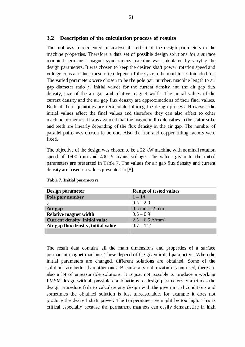
Table 7. Initial parameters

Design parameter Range of tested values

Pole pair number 1 – 14

0.5 – 2.0

Air gap 0.5 mm – 2 mm

Relative magnet width 0.6 – 0.9

Current density, initial value 2.5 – 6.5 A/mm2

Air gap flux density, initial value 0.7 – 1 T

The result data contains all the main dimensions and properties of a surface

permanent magnet machine. These depend of the given initial parameters. When the

initial parameters are changed, different solutions are obtained. Some of the

solutions are better than other ones. Because any optimization is not used, there are

also a lot of unreasonable solutions. It is just not possible to produce a working

PMSM design with all possible combinations of design parameters. Sometimes the

design procedure fails to calculate any design with the given initial conditions and

sometimes the obtained solution is just unreasonable, for example it does not

produce the desired shaft power. The temperature rise might be too high. This is

critical especially because the permanent magnets can easily demagnetize in high

52

temperatures. Therefore, checking is needed before the analysis to exclude

unreasonable solutions from the analysis. The checked properties are the produced

shaft power, the current density and linear current density, the temperature rise in the

magnets and the stator yoke height.

Because there are many varying parameters and a lot of data, it is difficult to

represent the data illustratively. A lot of different plotting methods were tested and

two were considered to be the most useful. One way is to plot the different solutions

as a function of certain properties, for example efficiency or mass. Another way is to

plot the interesting machine properties as a function of the initial parameters. Either

single solutions can be plotted or minimum, mean and maximum values of the

investigated parameter can be calculated from the solution data set. It was decided to

plot the investigated four parameters as functions of each other. The four properties

were also represented as a function of the six initial parameters.

The dimensioning tool works actually best with pole pair numbers 1 – 6 because the

machine constant is represented only for those pole pair numbers in [8]. It is possible

to do the dimensioning for larger pole pair numbers as well, but this means that the

curve has to be extrapolated.

Another problem with larger pole pair numbers is that the stator yoke often becomes

very thin. The reason for this is that the stator yoke height is calculated from the

chosen magnetic flux density value. If the yoke is very thin, it is not mechanically

strong enough. Therefore, the solutions with very thin yoke were left out of the

analysis.

This means that a smaller amount of good solutions were obtained with larger pole

pair numbers than smaller ones. For example if we look at Figure 11 the largest pole

pair number 14 is represented with dark blue dots. From the figure it can be seen that

there are quite a lot less data points for 28 pole machines than for example 24 pole

machines. In fact, 14 was the largest pole pair number that gave reasonable solutions

with this dimensioning tool. The main reason for this is the automatic choice of the

machine constant. If the dimensioning tool is used to calculate only one solution, the

machine constant can be chosen manually, and larger pole pair numbers are possible

as well.

The air gap flux densities for the stator yoke and teeth are also defined as initial

parameters. To reduce the number of varying parameters, they were assumed to be

linearly dependent of the flux density in the air gap. Therefore it has to be notified

that the air gap flux density initial parameter actually affects also the other flux

densities and not just the flux density in the air gap.

53

3.3 Machine properties explored

The most interesting machine properties are the efficiency, power factor, machine

size and weight and the amount of permanent magnet material used. The calculated

solutions of the result data set can be compared by observing these properties and

investigating how the initial parameters affect. The functioning of the machine is

investigated also in other operation points than the nominal point. Here the main

interests are the average efficiency and power factor during the working period.

These values are also included in the analysis. The chosen operation profile was

explained in Section 2.3.

If the efficiency is poor, it means that the machine has high losses, which means that

a lot of energy will be wasted. From the energy conservation point of view, the

efficiency should thus be as good as possible. Typically the efficiency of a

permanent magnet synchronous machine is high, about 0.9-0.95.

The power factor is the ratio of active and apparent power. A poor power factor

means that the machine needs a lot of reactive power. It is possible to achieve unity

power factor with a PMSM, even though sometimes lower power factors are also

used to improve other machine properties. For example the amount of permanent

magnet material can be reduced by allowing the back-EMF to be lower, for example

90 % of the phase voltage. This will also cause a lower power factor, but the

manufacturing costs are reduced. [7] Here it must be mentioned that the supply

voltage is assumed to be sinusoidal. With non-sinusoidal supply voltages, the power

factor would be less than one.

The weight of the machine should preferably be as small as possible. The lighter the

machine is, the less material is needed which makes the costs lower. Especially if the

machine is intended for a moving solution, for example an electric vehicle, the

weight of the machine can be a problem. In that kind of application part of the torque

produced by the machine goes to move the machine itself. If the machine can be

made to have less weight, less energy is needed to move the machine. Reduction of

the amount of material used is also environmentally friendly.

The permanent magnet materials are usually expensive. For example compared to

the price of copper, the price of NdFeB-magnet material is about 11 times higher [2],

[3]. This means that the amount of magnet material used should be small. However,

the magnets have to be thick enough to produce enough flux in the air gap.

Sometimes also the eddy current losses of the magnets might become large if the

magnets are small.

54

3.4 Effects of the initial design parameters

In this chapter, the obtained results are presented. The interesting properties are

efficiency, power factor, machine size and the amount of permanent magnet

material. For efficiency and power factor, both nominal and average values are

presented. The interesting properties are presented as functions of the design

parameters. Next, the effects of the investigated design parameters are presented.

3.4.1 Pole pair number

The dependency of the mass of a machine on its pole pair number is presented in

Figure 13. The leftmost figure represents the mass of the iron parts, i.e. the stator and

rotor core. The mass of the winding is presented in the middle and the total mass of

the machine in the rightmost figure in Figure 13. The pole pair number has a strong

effect on the machine size. The minimum mass obtained for a two-pole solution was

120 kg whereas the minimum mass for a 28-pole solution was only 25 kg. Also the

mean and maximum values of the weight of the iron parts decrease strongly when

the number of poles increases. From Figure 11, it can be seen that the solutions that

have two poles are considerably heavier than the other ones. This is because those

designs have a smaller machine constant than designs with larger pole pair number.

The definition of the machine constant is explained in Section 2.1.1 and Section 2.2.

According to the figure that is presented in [8] the machine constant for two-pole

machines is smaller than for other pole pair numbers. This choice makes the machine

larger, since the machine constant affects the machine size.

On the other hand, the efficiency becomes worse with the solutions having more

poles as can be seen from Figure 12. The best efficiency that was obtained was 0.966

with two poles whereas with 28 poles it was 0.916. The maximum power factor was

1 with all tested pole pair numbers. The power losses are presented in Figure 15,

which shows the total power losses as well as the iron and copper losses. It can be

observed that the iron losses become larger with larger pole pair numbers. This is

quite a natural result since the iron losses are calculated using Equation (82) which

depends of the frequency. Because the rotation speed is kept constant in this case, the

designs with higher pole pair number need a higher supply frequency as well. The

copper losses can be seen in the middle in Figure 15. It seems that there is a

minimum for the copper losses somewhere around pole pair number 5. However, the

total losses behave quite similarly with the iron losses. It can be also seen that with

small number of poles, the copper losses are larger than the iron losses whereas with

larger number of poles the iron losses become larger due to the increased frequency.

55

Figure 11. Efficiency and mass of iron parts with different number of poles.

Figure 12. The effect of the pole pair number.

0 50 100 1500.84

0.86

0.88

0.9

0.92

0.94

0.96

0.98

Mass of the iron parts (kg)

Eff

icie

ncy

p = 1

p = 2

p = 3

p = 4

p = 5

p = 6

p = 8

p = 10

p = 12

p = 14

2 4 6 8 10 12 14

0.86

0.88

0.9

0.92

0.94

0.96

Eff

icie

ncy

Pole pair number

Min Mean Max

0 5 10 150.85

0.9

0.95

1

Pow

er f

acto

r

Pole pair number2 4 6 8 10 12 14

2

4

6

8

10

12

14

16

x 10-4

Am

ount

of

per

man

ent

mag

net

mat

eria

l (m

3)

Pole pair number

56

Figure 13. The mass of the different designs as a function of the pole pair number.

Figure 14. Average efficiency and power factor as a function of pole pair number.

The working temperatures of the different machine parts are represented in Figure

16. It is worth mentioning here that the temperatures of a single solution are not

0 5 10 150

20

40

60

80

100

120

140

160

Pole pair number

Mas

s of

iron p

arts

(kg)

Min Mean Max

0 5 10 150

5

10

15

20

25

30

35

40

Pole pair number

Mas

s of

the

win

din

g (

kg)

0 5 10 1520

40

60

80

100

120

140

160

180

200

Pole pair number

Tota

l m

ass

(kg)

2 4 6 8 10 12 14

0.84

0.86

0.88

0.9

0.92

0.94

0.96

Pole pair number

Aver

age

effi

cien

cy

Min Mean Max

0 5 10 150.85

0.9

0.95

1

Pole pair number

Aver

age

pow

er f

acto

r

57

presented and Figure 16 shows only the minimum, average and maximum

temperatures of the set of obtained design solutions. Anyhow the temperatures seem

to rise when the number of poles is increased. This is quite logical since the iron

losses increase also. It can be also seen that the winding and endwinding have the

highest temperature.

Figure 15. Power losses as a function of the pole pair number.

The curve for the amount of permanent magnet material used looks quite interesting

(see Figure 12). It seems that less magnet material is needed with larger pole pair

numbers. However, the maximum value for the volume of permanent magnets rises

quite dramatically when the pole pair number is 8. It must be noticed that when

studying the amount of permanent magnet material, the solutions with minimum

value are optimal, and the ones with large values are expensive. Because any kind of

optimization algorithm is not used, there are both good and bad solutions presented

in the figures. This causes a large variation between the maximum and minimum

values of some of the investigated properties. The amount of permanent magnet

material depends on the magnet thickness. The dimensioning tool solves the

thickness iteratively as shown in the flowchart in Figure 7 (steps 9 – 18). To be able

to calculate a great amount of different solutions, the permanent magnet thickness

was limited to 50 mm at maximum, which is quite a large value. This value was

chosen because it ensures that the iteration does not stop too early. Sometimes it can

happen that the iteration does not converge. This then means that not even magnets

as thick as 50 mm are able to produce the wanted back-EMF for the design in

question. This could be one possible explanation for the rapid change in the amount

of permanent magnet material in Figure 12.

2 4 6 8 10 12 14

500

1000

1500

2000

2500

3000

Pole pair number

Iro

n l

oss

es (

W)

Min Mean Max

5 10 15

400

600

800

1000

1200

1400

Pole pair number

Co

pp

er l

oss

es (

W)

5 10 15

1000

1500

2000

2500

3000

3500

Pole pair number

To

tal

po

wer

lo

sses

(W

)

58

Figure 16. The temperatures of the different machine parts as a function of the pole

pair number. Minimum, mean and maximum values are presented.

It is noteworthy too that the minimum and mean values of magnet material decrease

when there are more poles. Therefore, it is possible to reduce the amount of magnet

material needed by adding more poles.

3.4.2 Machine length to air gap diameter ratio

Figure 17 shows how the machine length to air gap ratio affects the investigated

machine properties. The mass of the machine is presented in Figure 18 and Figure 19

shows the average efficiency and power factor. is varied from 0.5 to 2. This means

that the machine length can vary between half of the air gap diameter to twice the air

gap diameter. It can be seen that the machine is lighter when the air gap diameter is

large compared to the machine length. For example when the machine length is only

half of the air gap diameter, an average weight of 60 kg was obtained for the

solutions whereas when the machine length was twice the air gap diameter the

average weight was about 95 kg. Also the obtained minimum weight increased from

20 kg to 50 kg.

On the other hand, the efficiency is worse with short and thick machines than with

long and thin machines although the differences are rather small. When is

increased from 0.5 to 2 the best obtained efficiency increases from 0.960 to 0.965.

When increases the amount of permanent magnet material increases as well. The

maximum value of the power factor is one with every tested machine length to air

0 5 10 1540

50

60

70

80

90

100

110

Pole pair number

Min

imu

m t

emp

erat

ure

s (o

C)

Frame Yoke Teeth Winding Endwinding Magnets Bearings

0 5 10 1540

50

60

70

80

90

100

110

120

130

Pole pair number

Mea

n t

emp

erat

ure

s (o

C)

0 5 10 1540

60

80

100

120

140

160

180

200

220

Pole pair number

Max

imu

m t

emp

erat

ure

s (o

C)

59

gap ratio values. The mean value is also high, above 0.98. The average efficiency

(Figure 19) behaves quite similarly with the nominal efficiency.

Figure 17. The effect of the machine length to air gap diameter ratio on the nominal

efficiency, power factor and permanent magnet volume.

Figure 18. The mass of the different designs as a function of the machine length to air

gap diameter ratio .

1 2

0.86

0.88

0.9

0.92

0.94

0.96E

ffic

iency

Machine length toair gap diameter ratio

Min Mean Max

0.5 1 1.5

0.86

0.88

0.9

0.92

0.94

0.96

0.98

1

Pow

er f

acto

r


0.5 1 1.5

2

4

6

8

10

12

14

16

x 10-4

Am

ount

of

per

man

ent

mag

net

mat

eria

l (m

3)


1 2

20

40

60

80

100

120

140


Mas

s o

f ir

on

par

ts (

kg

)

Min Mean Max

1 2

5

10

15

20

25

30

35


Mas

s o

f th

e w

ind

ing

(k

g)

1 220

40

60

80

100

120

140

160

180


To

tal

mas

s (k

g)

60

Figure 19. The average efficiency and power factor as a function of machine length to

air gap ratio.

3.4.3 Air gap

The effect of the air gap length δ on the machine properties is discussed next. The

actual air gap is measured from the top surface of the permanent magnets to the

bottom of the stator teeth. The lower limit for the air gap length is set by the

mechanical constraints. Basically the upper limit is not as clear, but if the air gap

becomes too large, the magnets cannot produce enough flux to cause the rotor to

rotate.

The air gap length can be also evaluated from Equations (14) and (15) which depend

on the desired shaft power of the machine. Here the air gap was considered as a free

design parameter, and its value was varied. This is partly because the air gap given

by (14) and (15) is very small, about 0.5 mm for a 22 kW machine with more than

two poles. This is maybe some kind of theoretical minimum value for the air gap,

and therefore it was used as a lowest value that was tested.

The effect of the air gap is shown in Figure 20 and Figure 21. The air gap varies

from 0.5 mm to 2.5 mm. The smallest value is probably somewhat theoretical but it

is close to the value obtained with Equations (14) and (15). It was still tested despite

the fact that it is maybe always not realistic.

0.5 1 1.5 20.82

0.84

0.86

0.88

0.9

0.92

0.94

0.96

0.98

1


Av

erag

e ef

fici

ency

Min Mean Max

0.5 1 1.5 20.85

0.9

0.95

1


Av

erag

e p

ow

er

fact

or

61

Figure 20. The effect of the air gap to the machine properties.

Figure 21. The effect of the air gap on the mass of the machine.

It can be seen from Figure 21 that the mass of the machine becomes slightly smaller

with larger air gaps. However the effect is not very strong. The efficiency is better

with larger air gaps although the obtained maximum value increases only slightly.

The power factor is worse if the air gap is larger although the maximum value is

0 1 2 30.84

0.86

0.88

0.9

0.92

0.94

0.96

0.98

Eff

icie

ncy

Air gap (mm)

Min Mean Max

0 1 2 30.85

0.9

0.95

1

Pow

er f

acto

r

Air gap (mm)0 1 2 3

0

0.2

0.4

0.6

0.8

1

1.2

1.4

1.6

1.8x 10

-3

Am

ount

of

per

man

ent

mag

net

mat

eria

l (m

3)

Air gap (mm)

0 1 2 30

20

40

60

80

100

120

140

160

Air gap (mm)

Mas

s of

iron p

arts

(kg)

Min Mean Max

0 1 2 30

5

10

15

20

25

30

35

40

Air gap (mm)

Mas

s of

the

win

din

g (

kg)

0 1 2 320

40

60

80

100

120

140

160

180

200

Air gap (mm)

Tota

l m

ass

(kg)

62

always one. The minimum and mean values decrease slightly when the air gap

increases. The average efficiency and power factor behave similarly than the

nominal values as can be seen from Figure 22.

Figure 22. The average efficiency and power factor versus the air gap of the machine.

3.4.4 Relative magnet width

The relative magnet width describes how wide the magnets are compared to the pole

pitch. The actual width of the magnets is here obtained by multiplying the pole pitch

by the relative magnet width. According to [9] typical relative permanent magnet

width for surface mounted permanent magnet machines is about 0.8–0.85. Here the

relative magnet width was varied between 0.6 and 0.9.

The effect of the relative magnet width is shown in Figure 23, Figure 24 and Figure

25. The relative magnet width does not seem to have very strong effect on any of the

investigated properties. The total mass of the designs seem to increase slightly when

the relative magnet width is increased. This is because of the increased mass of the

iron parts. The mass of the winding is actually smaller with wider magnets. The

magnet width also affects the torque ripple.

0.5 1 1.5 2 2.50.82

0.84

0.86

0.88

0.9

0.92

0.94

0.96

0.98

1

Air gap (mm)

Aver

age

effi

cien

cy

Min Mean Max

0.5 1 1.5 2 2.50.85

0.9

0.95

1

Air gap (mm)

Aver

age

pow

er f

acto

r

63

Figure 23.The machine properties as a function of the relative magnet width.

Figure 24. The effect of the relative magnet width on the mass of the machine.

0.6 0.7 0.8 0.9

0.86

0.88

0.9

0.92

0.94

0.96

Eff

icie

ncy

Relative magnet width

Min Mean Max

0.7 0.8 0.9

0.86

0.88

0.9

0.92

0.94

0.96

0.98

1

Pow

er f

acto

r

Relative magnet width0.6 0.7 0.8 0.9

2

4

6

8

10

12

14

16

x 10-4

Am

ount

of

per

man

ent

mag

net

mat

eria

l (m

3)


0.6 0.7 0.8 0.9

20

40

60

80

100

120

140


Mas

s of

iron p

arts

(kg)

Min Mean Max

0.6 0.7 0.8 0.9

5

10

15

20

25

30

35


Mas

s of

the

win

din

g (

kg)

0.6 0.7 0.8 0.920

40

60

80

100

120

140

160

180


Tota

l m

ass

(kg)

64

Figure 25. The weighted averages of the efficiency and the power factor as a function of

the relative magnet width.

3.4.5 Current density

The effect of the initial value of stator winding current density is presented in Figure

26, Figure 27 and Figure 29. The initial value of the current density is a guess that is

used to calculate the stator current. If a higher initial value is allowed, the current

becomes higher which means that the losses should also be higher. Figure 28 shows

how the obtained final current density depends on its initial value. The final value

correlates quite well with the initial current density. It seems that the deviation is

about from the initial value.

The increase in the initial value of current density indeed decreases the efficiency.

The maximum value obtained decreases from 0.966 to 0.948. Also the mass of the

designs decreases when the current density increases. The effect is strongest on the

mass of the windings but also the mass of the iron parts decreases as can be seen

from Figure 27.

0.6 0.7 0.8 0.9

0.84

0.86

0.88

0.9

0.92

0.94

0.96


Aver

age

effi

cien

cy

Min Mean Max

0.6 0.7 0.8 0.9

0.86

0.88

0.9

0.92

0.94

0.96

0.98

1


Aver

age

pow

er f

acto

r

65

Figure 26.The effect of the initial value of the current density in the stator.

Figure 27. The effect of the current density on the mass of the machine.

The current density has an effect on the amount of permanent magnet material too.

For example the minimum value was reduced from m3 to

m3 when the current density was increased from 2.5 A/mm

2 to 6.5 A/mm

2.

2 4 6

0.86

0.88

0.9

0.92

0.94

0.96

Eff

icie

ncy

Current density,

intial value (A/mm2)

Min Mean Max

4 6

0.86

0.88

0.9

0.92

0.94

0.96

0.98

1

Pow

er f

acto

r

Current density,


4 6

2

4

6

8

10

12

14

16

x 10-4

Am

ount

of

per

man

ent

mag

net

mat

eria

l (m

3)

Current density,


4 6

20

40

60

80

100

120

140

Current density,


Mas

s o

f ir

on

par

ts (

kg

)

Min Mean Max

4 6

5

10

15

20

25

30

35

Current density,


Mas

s o

f th

e w

ind

ing

(k

g)

4 620

40

60

80

100

120

140

160

180

Current density,


To

tal

mas

s (k

g)

66

The maximum power factor is always one, but the mean value increases when the

current density increases. However, the average power factor decreases even if the

nominal one increases. The average efficiency is rather close to the nominal one.

Figure 28. The dependency of the stator current density on the given initial value.

Figure 29. Average efficiency and power factor as a function of the initial value for

current density.

2.5 3 3.5 4 4.5 5 5.5 6 6.52

3

4

5

6

7

8

Current density, initial value (A/mm2)

Curr

ent

den

sity

, obta

ined

val

ue

(A/m

m2)

3 4 5 6

0.84

0.86

0.88

0.9

0.92

0.94

0.96

Current density,


Av

erag

e ef

fici

ency

Min Mean Max

3 4 5 6

0.86

0.88

0.9

0.92

0.94

0.96

0.98

1

Current density,


Av

erag

e p

ow

er

fact

or

67

3.4.6 Air gap flux density

The initial value of the air gap flux density affects also the flux densities in the stator

yoke and teeth. As was explained earlier, the choice of the other flux densities is

based on the initial value of the air-gap flux density. Also the desired linear current

density in the stator is calculated using the initial guess for the air gap flux density.

By allowing larger magnetic flux density in the machine, the machine size can be

reduced. However, sometimes there is a quite large difference between the initial

value of the air gap flux density and the realised one as can be seen from Figure 31.

This is because the realised air gap flux density is calculated iteratively as shown in

Figure 7.

Figure 30. The effect of the choice for the initial value of magnetic flux density in the

air gap.

0.8 1

0.86

0.88

0.9

0.92

0.94

0.96

Eff

icie

ncy

Air gap flux density,initial value (T)

Min Mean Max

0.8 1

0.86

0.88

0.9

0.92

0.94

0.96

0.98

1P

ow

er f

acto

r


0.8 1

2

4

6

8

10

12

14

16

x 10-4

Am

ount

of

per

man

ent

mag

net

mat

eria

l (m

3)


68

Figure 31. The effect of the initial value of air gap flux density on the mass of the

machine.

Figure 32. Air gap flux density initial and final values.

It can be seen from Figure 31 that by choosing a larger initial value for the magnetic

flux density in the air gap, the mass of the machine can be reduced. This applies to

both the mass of the iron parts and the mass of the winding. For example when the

initial value of the air gap flux is 0.7 T, the minimum obtained mass is 36 kg

0.8 1

20

40

60

80

100

120

140


Mas

s o

f ir

on

par

ts (

kg

)

Min Mean Max

0.8 1

5

10

15

20

25

30

35


Mas

s o

f th

e w

ind

ing

(k

g)

0.8 1

40

60

80

100

120

140

160

180


To

tal

mas

s (k

g)

0.65 0.7 0.75 0.8 0.85 0.9 0.95 10.45

0.5

0.55

0.6

0.65

0.7

0.75

0.8

0.85

0.9

0.95

Air gap flux density, initial value (T)

Air

gap

flu

x d

ensi

ty,

obta

ined

val

ue

(T)

69

whereas with air gap flux initial value 1.0 T the minimum obtained mass was 21 kg.

This is probably because the initial value of the magnetic flux density defines also

the magnetic flux densities in the stator yoke and teeth. By allowing a larger flux

density in the stator, the yoke and teeth become smaller, and the mass is thus

reduced.

However, Figure 30 shows that the obtained efficiency becomes smaller with larger

air gap flux density initial value. The power factor is better with higher initial values,

but the maximum value is still one. The amount of magnet material needed increases

when the magnetic flux value is increased. This is quite natural since the main flux is

produced by the permanent magnets. Like the nominal efficiency, the average

efficiency is also worse with larger air gap flux density values. The average power

factor behaves in a slightly different way though. The maximum value is one, but

there is quite much variation in the minimum value. The average value on the other

hand does not change very much which means that the variations in the minimum

values are probably caused by single solutions that can be considered as outliers with

respect to the average power factor.

Figure 33. The effect of air gap flux density initial value on the average efficiency and

power factor.

0.7 0.8 0.9 1

0.84

0.86

0.88

0.9

0.92

0.94

0.96


Av

erag

e ef

fici

ency

Min Mean Max

0.8 0.9 1

0.86

0.88

0.9

0.92

0.94

0.96

0.98

1


Av

erag

e p

ow

er

fact

or

70

4 Discussion

4.1 Conclusions

The results are combined in Table 8. The table shows what happens to the

investigated machine properties when the values of the different initial parameters

are increased. In most cases, the results agreed well with the FEM calculations.

However, there are still some differences in for example iron losses that have to be

investigated.

Table 8. Effect of initial parameters, 22 kW machine

Increasing

parameter

Efficiency Power

factor

Machine

size

Amount of

permanent magnet

material

Pole pair

number

decreases maximum 1 decreases decreases

increases maximum 1 increases increases

Air gap slightly

increases

maximum

value 1

slightly

decreases

slightly decreases

Relative magnet

width

no clear

effect

maximum 1 slightly

increases

no clear effect

Current density,

initial value

decreases maximum 1,

increases

decreases slightly decreases

Air gap flux

density, initial

value

decreases maximum 1,

increases

decreases increases

The effect of a change in the efficiency can be evaluated by calculating the energy

costs during a certain time interval, for example 10 years. According to [17] the

energy price for small industry is 4.34 c/kWh. The average power of the machine can

be calculated from the operation profile presented in Section 2.3. For a 22 kW

machine Equation (51) gives 8.39 kW for the average shaft power. If the efficiency

decreases for example from 0.94 to 0.93 the difference in the energy costs becomes

365 € in 10 years. If the decrease in the efficiency is 0.1, the energy costs increase

4500 €.

For the material costs, one estimate for NdFeB-magnet material is 62 €/kg [2]. If the

total volume of the magnets decreases 200 cm3, it means a 1.46 kg decrease in the

mass and a 90.52 € decrease in the material costs. The conclusion is that if the

machine is intended for long time use, the energy costs are larger and thus in this

case it is more important to obtain good efficiency than to reduce the magnet

volume.

71

Since the flux density in the stator yoke and teeth depends of the air gap flux density,

changing the latter one will affect also to the two other values. Therefore the air gap

flux density initial value can affect to the machine size. By increasing the air gap

flux initial value, it is possible to decrease the machine size. However, this leads to

decreased efficiency and increased amount of permanent magnet material.

This is reasonable, since the main flux is produced by the permanent magnets. The

machine size decreases since larger flux density is allowed in the stator. However,

the magnetic flux density cannot be made as large as possible, because when the flux

density becomes larger than a certain value, the iron starts to saturate. After that, the

flux density cannot be increased very much. According to the results, the optimal

value for the air gap flux density is a compromise between the machine size and the

amount of permanent magnet material used and efficiency.

The machine size can be decreased by increasing the current density. Also the

amount of permanent magnet material will decrease slightly. When larger current

density is allowed, it means that the conductors in the stator winding can be made

smaller. The thinner conductors need smaller area in the stator slots, which means

that the stator slots can be made smaller. This will also reduce the outer diameter of

the stator core and therefore also the mass of the iron parts. The major drawback is

that the efficiency decreases, presumably due to increased current losses. The power

factor is improved slightly, although unity power factor is possible with smaller

current densities as well.

The relative magnet width does not have very strong effect on any of the properties.

By decreasing the magnet width, it is possible to slightly decrease the mass of the

machine, but the effect is not very strong. The upper limit for the magnet width is the

pole pitch.

Increasing the air gap slightly increases the efficiency and decreases the machine

size, but the amount of permanent magnet material needed becomes larger. This

happens because when the air-gap is made larger, the distance between the magnets

and the stator winding increases, which means that thicker magnets are needed to

produce enough flux to cause the machine to rotate. However, it was noticed that if

the air gap was very small and the magnets were very thin, the eddy current losses in

the magnets became huge. The optimal size of the air gap is thus a compromise

between the machine size and the amount of permanent magnet material used. Its

effect on the power factor is not significant since unity power factor is possible to

achieve with any air gap size tested.

According to Table 8, if the increases, the amount of magnet material decreases.

The machine size seems to have minimum with somewhere in the middle. The

effect on the machine size is however indirect, and cannot be seen from these results,

since the machine constant is not varied here. With larger stator inner diameter, more

72

slots will fit in. This means that it is possible to obtain a linear current density that

corresponds to a larger machine constant and thus smaller machine.

Increasing the causes the efficiency and power factor to decrease. This means

basically that a shorter machine with larger diameter gives better efficiency and

power factor. Also the machine size can be reduced by increasing the machine

constant. The drawback of the larger value of is that more magnet material is

needed.

The number of poles affects strongly the size of the machine. With larger number of

poles the machine becomes smaller, but if the rotation speed is kept constant, higher

supply frequency is needed. For this reason the efficiency becomes worse with larger

pole pair number since the losses depend of the frequency. By choosing the other

parameters well, it is however possible to obtain a larger efficiency with larger

number of poles. The amount of permanent magnet material is smaller when there

are more poles.

The clearest results are the following:

- Increasing the number of poles will decrease both machine size and

efficiency

- Increasing the machine length to air gap diameter ratio will increase the

machine size and the amount of magnet material needed

- Larger initial value for the stator current density will decrease the machine

size and efficiency

- Increasing the initial value of the air gap flux density will increase the

amount of permanent magnet material needed

- The relative magnet width does not seem to have very strong effect on

anything

- Choosing a smaller air-gap decreases the thickness of the permanent magnets

- Increasing the machine length to air gap ratio increases the efficiency

The purpose of this study was to find contradictive design parameters that could be

used for optimization of a surface mounted permanent magnet synchronous machine.

There seems to be a contradiction between the efficiency and the machine size. The

machine size can be reduced by at least two ways: by increasing the pole pair

number or the stator current density. Both of these methods also increase the losses,

which means that the efficiency becomes worse. Also increasing the machine length

to air gap diameter ratio slightly improves the efficiency, but this means also

increased machine size and amount of permanent magnet material. The power factor

of a PMSM seems to be usually quite good which is also said in the literature.

73

4.2 Further work

With the dimensioning tool, it is possible to design a surface mounted permanent

magnet synchronous machine. The design results can be modified to meet different

requirements for different applications. It is easy to test how the results can be

modified by changing different parameters. It is also possible to calculate the basic

dimensioning for given initial conditions. It is rather easy to obtain a number of

possible design solutions for a given design situation by changing the free

parameters. The results can be used to analyse the design choices.

However, there are still some improvements that could be done. It is still somewhat

difficult to present the results illustratively. This is partly because the amount of data

is rather large, and partly because there are many varying parameters. One problem

is that all possible combinations of the initial parameters do not give a reasonable

design result. For example the obtained shaft power might become considerably

smaller than the desired one. This is often due to high losses.

This means that it is not possible to use all possible combinations in the analysis, and

during the results calculation process, also a lot of non-working solutions are

generated. These have to be filtered out before starting to analyse. It also makes it

more difficult to analyse the results. Because all the solutions are not optimal, the

data points in the figures do not form a clear line or curve. If some kind of

optimization algorithm would have been used, result data points would have formed

some kind of optimal curve.

It has to be also remembered that the machine design process has multiple properties

that have to be optimized. This means that the best solutions are always

compromises between different criteria. From the optimization point of view, it

could be useful, if some of the parameters could be combined somehow. One

possibility could be to investigate if the efficiency and power factor could be

combined. The optimal solution also depends on the application the machine is

intended for. Sometimes for example the machine price might not have a great

importance whereas the size could be critical. On some other cases however, the

costs should be reduced as much as possible, which could reduce the use of the

magnet material for instance.

In the example case of the 22 kW industrial pump, presumably the efficiency would

be important because the pump is working 70 % of the working period. If the

efficiency is poor, it means that losses are high which means that more energy is

wasted and the energy costs of the pump become higher. Because the pump is

designed for industrial use, it is presumably meant to last a rather long time. This

means that the production and material costs are less important than the operating

costs.

74

The conclusion is that to further improve the dimensioning tool, an optimization

algorithm should be used. This would help finding the good combinations of initial

parameters. However, without the optimization, it is possible to investigate also the

worse results and see what kind of initial parameter combinations result to these.

At the moment, the dimensioning tool supports only surface mounted machines with

single layer winding. These constructions were chosen for simplicity. With rather

simple modifications, it would be possible to get the tool work also with double layer

windings. This would make it also possible to compare different winding types with

each other.

75

References

1. Morimoto, S. Trends of Permanent Magnet Synchronous Machines.

Transactions on Electrical and Electronic Engineering 2007, Vol. 2.

2. Gieras, J.F. & Wing, M. Permanent Magnet Motor Technology - Design and

Applications. Marcel Dekker, Inc, 2002.

3. Current Primary and Scrap Metal Prices, Available:

http://www.metalprices.com/#, Accessed 04.05.2012.

4. MathWorks/MATLAB Web Page, Available:

www.mathworks.com/products/matlab/, Accessed 03.05.2012.

5. Puranen, J. Induction Motor Versus Permanent Magnet Synchronous Motor in

Motion Control Applications: a Comparative Study, Doctoral Thesis,

Lappeenranta University of Technology, Acta Universitatis Lappeenrantaensis

249, 2006.

6. Guru, B.S. & Hiziroǧlu, H.R. Electric Machinery and Transformers. 3rd ed.

Oxford University Press, 2001. 726.

7. Heikkilä, T. Permanent Magnet Synchronous Motor for Industrial Inverter

Applications - Analysis and Design. Dissertation, Lappeenranta University of

Technology, Acta Universitatis Lappeenrantaensis 134, 2002.

8. Pyrhönen, J., Jokinen, T. & Hrabovcová, V. Design of Rotating Electrical

Machines. John Wiley & Sons, Ltd., 2008.

9. Jussila, H. Napakäämityn murtovakokestomagneettitahtikoneen suunnittelu.

Master's Thesis, Lappeenranta University of Technology, 2005.

10. Demetriades, G.D., Zelaya de la Parra, H., Andersson, E. & Olsson, H. A

Real-Time Thermal Model of a Permanent Magnet Synchronous Motor. IEEE

Transactions on Power Electronics 2010, Vol. 25, No. 2

11. Hafner, M., Schöning, M. & Hameyer, K. Automated sizing of permanent

magnet synchronous machines with respect to electromagnetic and thermal

aspects. COMPEL: The International Journal for Computation and Mathematics

in Electrical and Electronic Engineering 2010, Vol. 25, No. 9.

12. Lindström, J., Thermal Model of a Permanent-Magnet Motor for a Hybrid

Electric Vehicle. Department of Electric Power Engineering, Chalmers

University of Technology, Göteborg, Sweden, 1999. Report No. 11R, ISSN:

1401-6176.

76

13. El-Refaie, A.M., Harris, N.C., Jahns, T.M. & Rahman, K.M. Thermal analysis

of multibarrier interior PM synchronous Machine using lumped parameter

model. IEEE Transactions on Energy Conversion 2004, Vol. 19, No. 2.

14. Kylander, G. Thermal modelling of small cage induction motors. Doctoral

Thesis, Chalmers University of Technology, Göteborg, Sweden, 1995.

15. CEDRAT homepage, Available: www.cedrat.com, Accessed 09.05.2012.

16. Keränen, J.S. Calculation of validation data for permanent magnet machine

dimensioning tool. Extended Abstract, TK3047 Electrical Product Concepts

Team Workshop, Espoo: 2012.

17. Web Page of Energiamarkkinavirasto, Available:

www.energiamarkkinavirasto.fi, Accessed 11.05.2012.

18. Piippo, A., Hinkkanen, M. & Luomi, J. Sensorless Control of PMSM Drives

Using a Combination of Voltage Model and HF Signal Injection.

Conference Record of the 39th IEEE-Industry Applications Society (IAS)

Annual Meeting. Vol. 2. 2004.

19. Pillay, P. & Krishnan, R. Modeling of Permanent Magnet Motor Drives. IEEE

Transactions on Industrial Electronics 1988, Vol. 34, No. 4.

Appendix 1: Explanation of the d- and q-axis and the

inductances

The synchronous machine is often presented using a two-axis model where the direct

axis (d-axis) is in the direction of the pole and quadrature axis (q-axis) between the

two poles. The equivalent circuit for a synchronous machine can be presented for d-

and q-axis separately. The voltage equations for the d- and q-axis can be written as

[18]

(A1)

(A2)

and the flux equations as

(A3)

(A4)

where and are the d- and q- components of the stator voltage, and are the

d- and q-components of the stator current, and the components of the flux

linkage and is the flux produced by the permanent magnets. is the stator

resistance and and are the d- and q-axis inductances.

An equivalent circuit model is presented in Figure 1. [19]

Figure 1. Equivalent circuit of a PMSM in d- and q-axis.

The inductances of the d- and q-axis consist of the magnetizing inductances ,

and the leakage inductance . The inductances at steady state are presented in

Figure 2.

Figure 2. Inductances in the d- and q-axis at steady state.

Appendix 2: Dimensions and other parameters for

validated models

Three models were validated. The shaft power was set to 22 kW, rotation speed to

1500 rpm, and phase voltage to 230 V for all three designs. The first design had 2

poles, the second one 8 poles and the third one 14 poles. The dimensions given by

the dimensioning tool are given below for the three models.

Dimensions for a 2-pole design

FINAL DESIGN

PHASE VOLTAGE (V) 230.94

NOMINAL SPEED (rpm) 1500.00

MACHINE CONSTANT (Ws/m^3) 111185.00

Number of poles (-) 2

Supply frequency (Hz) 25.00

Effective length (mm) 318.1119

Actual length (mm) 313.1119

Actual air gap (mm) 2.5000

Stator outer diameter (mm) 308.8143

Stator inner diameter (mm) 159.0560

Number of slots (-) 48

Stator yoke height (mm) 50.7160

Filling factor for iron (-) 0.9500

Dimensions of the stator slots

H1 (mm) 24.1632

H11 (mm) 1.0000

H13 (mm) 18.2566

B11 (mm) 4.0675

B12 (mm) 5.4233

B13 (mm) 7.8131

Rotor outer diameter (mm) 143.5560

Permanent magnet width (mm) 169.3934

Permanent magnet thickness (mm) 5.2500

Number of phases (-) 3

Number of parallel paths (-) 1

Conductors in a slot (-) 8

Conductor area (cross sect.)(mm^2) 13.8874

Slot filling factor (-) 0.6000

Stator current (A) 35.9254

Shaft power at nominal speed (W) 22072.46

Torque at nominal speed (Nm) 140.52

Rotational speed (1/min) 1500.00

Air-gap flux density (T) 0.6297

Air-gap flux (Wb) 0.0339

eta at nominal speed (-) 0.9474

cos(phi) at nominal speed (-) 0.9361

Current density (A/mm^2) 2.5869

Losses

St. winding resistive (W) 489.63

Iron (W) 174.93

Additional (W) 167.78

Windage and ventilation (W) 81.83

Total (W) 1226.42

Stator resistance (ohm) 0.1265

D-axis inductance (H) 0.0306

Q-axis inductance (H) 0.0306

Temperatures

Frame 40.0423

Yoke 42.2870

Teeth 44.6464

Winding 51.8297

Endwinding 75.8694

Magnets 59.6648

Bearings 41.8995

Dimensions for the 8-pole design

FINAL DESIGN















H1 (mm) 26.8762

H11 (mm) 1.0000

H13 (mm) 20.4807

B11 (mm) 4.5825

B12 (mm) 6.1099

B13 (mm) 8.7909


















Losses


Iron (W) 355.86



Total (W) 1181.30




Temperatures

Frame 40.2370

Yoke 41.6610

Teeth 44.3529

Winding 55.3147

Endwinding 69.9706

Magnets 58.1568

Bearings 42.3544

Dimensions for the 14-pole design

FINAL DESIGN















H1 (mm) 16.4750

H11 (mm) 1.0000

H13 (mm) 12.1918

B11 (mm) 2.7407

B12 (mm) 3.6543

B13 (mm) 4.5663


















Losses


Iron (W) 639.98



Total (W) 1552.69




Temperatures

Frame 40.4734

Yoke 43.6688

Teeth 46.7270

Winding 72.4993

Endwinding 96.7940

Magnets 52.4083

Bearings 42.3090

Date post:	03-Feb-2022
Category:	Documents
Upload:	others
View:	1 times
Download:	0 times

Evaluation of the effects of design choices on surface mounted

Documents