195
NUREG/CR-6986 PNNL-13810 Evaluations of Structural Failure Probabilities and Candidate Inservice Inspection Programs Office of Nuclear Regulatory Research
NUREG/CR-6986 PNNL-13810
Evaluations of Structural Failure Probabilities and Candidate Inservice Inspection Programs
Office of Nuclear Regulatory Research


NUREG/CR-6986 PNNL-13810
Evaluations of Structural Failure Probabilities and Candidate Inservice Inspection Programs Manuscript Completed: November 2008 Date Published: May 2009 Prepared by M.A. Khaleel and F.A. Simonen
Pacific Northwest National Laboratory P.O. Box 999 Richland, WA 99352 D.A. Jackson and W.E. Norris, NRC Project Managers
NRC Job Code N6398 Office of Nuclear Regulatory Research
Abstract
The work described in this report applies probabilistic structural mechanics models to predict the reliability of nuclear pressure boundary components. These same models are then applied to evaluate the effectiveness of alternative programs for inservice inspection to reduce these failure probabilities. Results of the calculations would support the development and implementation of risk-informed inservice inspection of piping and vessels. Studies have specifically addressed the potential benefits of ultrasonic inspections to reduce failure probabilities associated with fatigue crack growth and stress-corrosion cracking. Parametric calculations were performed with the computer code pc-PRAISE to generate an extensive set of plots to cover a wide range of pipe-wall thicknesses, cyclic operating stresses, and inspection strategies. The studies have also addressed critical inputs to fracture mechanics calculations such as the parameters that characterize the number and sizes of fabrication flaws in piping welds. Other calculations quantify uncertainties associated with the inputs to the calculations, the uncertainties in the fracture mechanics models, and the uncertainties in the resulting calculated failure probabilities. A final set of calculations address the effects of flaw-sizing errors on the effectiveness of inservice inspection programs.
iii

iv
Foreword
The goal of inservice inspection (ISI) of nuclear reactor piping and pressure vessels is to reliably detect service- related defects in a timely manner and thereby maintain the structural integrity of the inspected components. As nuclear power plants have aged and instances of unexpected materials degradation have been reported, a goal of the nuclear industry has increasingly been to predict component degradation before it occurs. In addition to assessing potential degradation mechanisms and identifying components and materials that are expected to experience degradation, a proactive approach must consider inspection. The U.S. Nuclear Regulatory Commission (NRC), in an effort to assess the effectiveness of ISI programs, has supported research at Pacific Northwest National Laboratory (PNNL) to evaluate the reliability and accuracy of ISI, and recommend improvements to nondestructive examination (NDE) methods and requirements. The results from another program at PNNL, a study to collect estimates of failure probability and their associated uncertainties for passive reactor components, were published in May 2007 in NUREG/CR-6936, entitled “Probabilities of Failure and Uncertainty Estimate Information for Passive Components – A Literature Review.” Probabilistic fracture mechanics (PFM) models have been used for reliability analyses. Performance demonstrations have been implemented to upgrade the quality of ultrasonic testing (UT) by addressing the key elements needed for effective inspections—namely, personnel, procedures, and equipment. This report presents the results of a study to (1) apply PFM models to predict component failure probabilities by modes ranging from leaks to rupture, and (2) evaluate the potential effectiveness of ISI to reduce such failure probabilities. A PFM model was used to simulate the effects of flaw detection and sizing errors that may occur during vessel and piping inspections. That model was then used to perform calculations for a range of representative values of flaw detection probabilities, flaw sizing errors, and flaw acceptance criteria. The candidate inspection programs considered three different levels of NDE reliability and different inspection frequencies. A collection of curves was generated that describes the effects of inservice inspections on piping reliability. The curves can be used to identify optimum inspection strategies for specified conditions of cyclic stresses. The calculations show that high-quality inservice inspections can significantly reduce leak and break probabilities, particularly if the inspections are performed relatively frequently. It was also shown that preservice inspections can be effective in reducing leak probabilities and failures. Probability of detection (POD) capability appears to be the most limiting factor with regard to the overall capability of ISI to reduce leak probabilities. Results from the research have been used to support development of NRC guidance for implementation of risk-informed ISI of piping. The results have also been used in the development of PFM tools to generate failure probabilities for vessels that has been used in regulatory decision making.
v

vi
Contents
Abstract ........................................................................................................................................................iii Foreword....................................................................................................................................................... v Executive Summary ...................................................................................................................................xix Acknowledgments....................................................................................................................................xxiii Abbreviations and Acronyms ................................................................................................................... xxv 1 Introduction ...................................................................................................................................... 1.1 2 Flaw-Size Distribution and Flaw-Existence Frequencies in Nuclear Piping ................................... 2.1
2.1 Introduction ............................................................................................................................ 2.1 2.2 Summary of Past Works......................................................................................................... 2.2 2.3 Flaw-Distribution Model........................................................................................................ 2.3
2.3.1 Centerline Cracking................................................................................................... 2.5 2.3.2 Heat-Affected Zone Cracking ................................................................................... 2.5 2.3.3 Lack of Fusion........................................................................................................... 2.6 2.3.4 Non-Metallic Slag Inclusions.................................................................................... 2.6 2.3.5 Porosity...................................................................................................................... 2.6 2.3.6 Defect Density........................................................................................................... 2.6 2.3.7 Defect Characteristics................................................................................................ 2.8 2.3.8 Inspection Model....................................................................................................... 2.8
2.4 Computer-Based Implementation........................................................................................... 2.9 2.5 Inputs for Sensitivity Study.................................................................................................... 2.9 2.6 Results of Sensitivity Study ................................................................................................. 2.14 2.7 Defect Size Distributions...................................................................................................... 2.15
2.7.1 Procedure for Fitting of Statistical Distributions..................................................... 2.15 2.7.2 Resulting Lognormal Flaw-Depth Distributions ..................................................... 2.17 2.7.3 Effects of Weld Process on Depth Distribution ...................................................... 2.17
2.8 Flaw Depth Distribution Parameters versus Wall Thickness ............................................... 2.24 2.9 Number of Flaws versus Wall Thickness............................................................................. 2.26 2.10 Conclusions .......................................................................................................................... 2.28
3 Parametric Calculations for Fatigue................................................................................................. 3.1 3.1 Introduction ............................................................................................................................ 3.1 3.2 Piping Reliability Code pc-PRAISE ...................................................................................... 3.1 3.3 Flaw Size Distribution............................................................................................................ 3.4 3.4 Parametric Treatment of Cyclic Stresses Using the Q-Factor ................................................ 3.5 3.5 Results of Sensitivity Calculations......................................................................................... 3.6
3.5.1 Failure Probabilities versus Q-Factor........................................................................ 3.6 3.5.2 Effects of Through-Wall Stresses Gradients ............................................................. 3.9 3.5.3 Effect of Initial Flaw Length ................................................................................... 3.12 3.5.4 Effect of Sustained Primary Stress Level on Failure Probabilities ......................... 3.14 3.5.5 Effect of Abnormal/Seismic Stress Level on Failure Probabilities......................... 3.14 3.5.6 Effect of Leak Detection on Failure Probabilities ................................................... 3.17
vii
3.6 Summary and Conclusions................................................................................................... 3.19 4 Fatigue of Stainless Steel Piping...................................................................................................... 4.1
4.1 Introduction ............................................................................................................................ 4.1 4.2 Scope of Calculations............................................................................................................. 4.1 4.3 Definition of Input Parameters ............................................................................................... 4.3
4.3.1 Pipe Dimensions........................................................................................................ 4.3 4.3.2 Flaw-Depth Distributions .......................................................................................... 4.3 4.3.3 Aspect-Ratio Distribution.......................................................................................... 4.4 4.3.4 Crack Growth Rates .................................................................................................. 4.4 4.3.5 Failure Criterion for Pipe Leakage ............................................................................ 4.5 4.3.6 Failure Criterion for Pipe Break................................................................................ 4.5
4.4 Probability of Detection Curves ............................................................................................. 4.6 4.5 Sensitivity Calculations for Inspection Model ....................................................................... 4.7
4.5.1 Effect of Initial Flaw-Size Distribution..................................................................... 4.8 4.5.2 Effect of Time of the First Inspection ....................................................................... 4.8 4.5.3 Independent versus Correlated Inspections ............................................................... 4.9 4.5.4 Combined Preservice Inspections and Inservice Inspections .................................. 4.10
4.6 Results of Parametric Calculations....................................................................................... 4.13 4.6.1 Effects of Pipe Wall Thickness on Failure Probabilities......................................... 4.13 4.6.2 Effects of Pipe-Wall Thickness on Improvement Factor ........................................ 4.16 4.6.3 Improvement Factors for Various Pipe-Wall Thicknesses...................................... 4.18
4.7 Summary and Conclusions................................................................................................... 4.28 5 Intergranular Stress Corrosion of Stainless Steel Piping.................................................................. 5.1
5.1 Introduction ............................................................................................................................ 5.1 5.2 Stress-Corrosion Cracking Model .......................................................................................... 5.1
5.2.1 Crack Initiation Model .............................................................................................. 5.2 5.2.2 Crack-Growth Model ................................................................................................ 5.3 5.2.3 Residual Stresses ....................................................................................................... 5.4 5.2.4 Failure Criterion for Pipe Breakage and Leakage ..................................................... 5.4 5.2.5 Numerical Simulation................................................................................................ 5.5
5.3 Definition of Dσ Parameter..................................................................................................... 5.5 5.4 Calibration and Benchmarking of Model ............................................................................... 5.6 5.5 Inservice Inspection Model .................................................................................................... 5.9
5.5.1 POD Curves............................................................................................................... 5.9 5.5.2 Factor of Improvement............................................................................................ 5.12 5.5.3 Independent versus Dependent Inspections............................................................. 5.12 5.5.4 Multiple Defects in a Given Weld........................................................................... 5.13
5.6 Input Parameters for Parametric Calculations...................................................................... 5.13 5.7 Results of Parametric Calculations....................................................................................... 5.13
5.7.1 Predicted Leak Probabilities versus Dσ ................................................................... 5.15 5.7.2 Effect of Pipe Size on Leak Probabilities................................................................ 5.15 5.7.3 Effect of POD Curve and ISI Frequency on Improvement Factor .......................... 5.15 5.7.4 Improvement Factors for Small Pipe Size............................................................... 5.18 5.7.5 Improvement Factors for Intermediate Pipe Size.................................................... 5.18 5.7.6 Improvement Factors for Large Pipe Size............................................................... 5.19
viii
5.7.7 Effect of Pipe Size on Improvement Factor ............................................................ 5.19 5.7.8 Time Dependence of Calculated Failure Probabilities ............................................ 5.19
5.8 Conclusions .......................................................................................................................... 5.20 6 Uncertainty Analysis for Calculated Failure Probabilities of Piping Welds.................................... 6.1
6.1 Introduction ............................................................................................................................ 6.1 6.2 Sensitivity Calculations.......................................................................................................... 6.2 6.3 Uncertainty Calculations ........................................................................................................ 6.7
6.3.1 Inputs for Calculations .............................................................................................. 6.7 6.3.2 Computational Approach ........................................................................................ 6.11
6.4 Results of Uncertainty Calculations ..................................................................................... 6.11 6.5 Generalization of Uncertainty Calculations ......................................................................... 6.14 6.6 Conclusion............................................................................................................................ 6.17
7 Effects of Flaw-Sizing Errors on the Reliability of Vessels and Piping .......................................... 7.1 7.1 Introduction ............................................................................................................................ 7.1 7.2 PFM Model ............................................................................................................................ 7.2 7.3 Inservice Inspection Model .................................................................................................... 7.2 7.4 Simulation of Flaw-Sizing Errors........................................................................................... 7.3 7.5 Inputs to PFM Calculations .................................................................................................... 7.4 7.6 Results of Example Calculations............................................................................................ 7.6
7.6.1 Vessel Calculations ................................................................................................... 7.7 7.6.2 Piping Calculations ................................................................................................. 7.11
7.7 Summary and Conclusions................................................................................................... 7.11 8 Conclusions ...................................................................................................................................... 8.1 9 References ........................................................................................................................................ 9.1
ix
Figures
2.1 Welding Defects ........................................................................................................................... 2.4
2.2 Schematic Representation of Weld Build Up and the Position of Different Types of Crack-Like Defects ....................................................................................................................... 2.5
2.3 Complimentary Distribution of Flaw Depth on Normal Probability Paper for Case 1............... 2.16
2.4 Lognormal Complimentary Distribution of Flaw Depth for Case 1 ........................................... 2.18
2.5 Lognormal Complimentary Distribution of Flaw Depth for Case 2 .......................................... 2.18
2.6 Lognormal Complimentary Distribution of Flaw Depth for Case 3 .......................................... 2.19
2.7 Lognormal Complimentary Distribution of Flaw Depth for Case 6 .......................................... 2.19
2.8 Lognormal Complimentary Distribution of Flaw Depth for Case 7 .......................................... 2.20
2.9 Lognormal Complimentary Distribution of Flaw Depth for Case 10 ......................................... 2.20
2.10 Comparison of Simulated Flaw Depth Distributions for 1-in. Wall Pipe Welds ....................... 2.22
2.11 Comparison of Simulated Flaw Depth Distributions for Three Pipe Wall Thicknesses ............ 2.23
2.12 Comparison of Simulated Flaw Depth Distributions for Three Pipe Wall Thicknesses Plotted in Terms of a/t ................................................................................................................ 2.23
2.13 Median Flaw Size and Shape Parameter for MMAW ............................................................... 2.24
2.14 Median Flaw Size and Shape Parameters for TIG Weld ........................................................... 2.25
2.15 Flaw per Inch of Weld versus Wall Thickness .......................................................................... 2.27
2.16 Flaw per Inch of Weld versus Wall Thickness .......................................................................... 2.27
3.1 Schematic Diagram of Piping Failure Probability Calculations as Performed by pc PRAISE......................................................................................................................................... 3.3
3.2 Probability of Leak as a Function of Crack Growth Parameter Q = αN(∆σ)4 for Two Categories of Defect Populations.................................................................................................. 3.8
3.3 Probability of Break as a Function of the Leak Probability.......................................................... 3.9
3.4 Probability of Leak as a Function of Fatigue Crack Growth Parameter Q = αN(∆σ)4............... 3.10
3.5 Probability of Leak as a Function of Fatigue Crack Growth Parameter Q = αN(∆σ)4............... 3.10
3.6 Probability of Leak as a Function of Fatigue Crack Growth Parameter Q = αN(∆σ)4............... 3.11
3.7 Probability of Leak as a Function of Fatigue Crack Growth Parameter Q = αN(∆σ)4............... 3.11
3.8 The Effect of Sustained Primary Stress on Leak Probability with Crack Growth Parameter = αN(∆σ)4.................................................................................................................. 3.16
3.9 The Effect of Crack Growth Parameter = αN(∆σ)4 and the Abnormal Stress on the Leak Probability.......................................................................................................................... 3.16
x
3.10 Comparison Between the Peak Probability for a Sustained Primary Stress of 24 ksi and Abnormal Plus Primary Stress of 24 ksi with Crack Growth Parameter = αN(∆σ)4 ........... 3.17
3.11 Effect of Leak Detection Threshold on Leak and Break Probabilities ....................................... 3.18
4.1 The Effect of Initial Flaw Distribution on the Improvement Factors with Q = αN(∆σ)4.............. 4.8
4.2 The Effect of Arrival Time of First Inservice Inspection on the Leak Probability of Failure ........................................................................................................................................... 4.9
4.3 Improvement Factors for Independent and Correlated Inspections versus Q = αN(∆σ)4 for ISI Every 10 Years ................................................................................................................ 4.10
4.4 Improvement Factors for Independent and Correlated Inspections versus Q = αN(∆σ)4 for ISI Every 5 Years .................................................................................................................. 4.11
4.5 Improvement Factors for Independent and Correlated Inspections versus Q = αN(∆σ)4 for ISI Every 2 Years .................................................................................................................. 4.11
4.6 Improvement Factors for Independent and Correlated Inspections versus Q = αN(∆σ)4 for ISI Every Year....................................................................................................................... 4.12
4.7 Effect of Combined Preservice and Inservice Inspection on Improvement Factors Q = αN(∆σ)4................................................................................................................................ 4.12
4.8 Effect of Wall Thickness on Calculated Leak Probabilities for Stainless Steel Piping Assuming One Flaw per Weld and No Inservice Inspection with Q = αN(∆σ)4 ....................... 4.14
4.9 Effect of Wall Thickness on Calculated Break Probabilities for Fatigue of Stainless Steel Piping Assuming One Flaw per Weld and No Inservice Inspection with Q = αN(∆σ)4 ...................................................................................................................................... 4.14
4.10 Effect of Wall Thickness on Calculated Leak Probabilities for Stainless Steel Piping Assuming Number of Flaws per Weld from Flaw Simulation Model and No Inservice Inspection with Q = αN(∆σ)4 ..................................................................................................... 4.15
4.11 Effect of Wall Thickness on Calculated Break Probabilities for Fatigue of Stainless Steel Piping Assuming Number of Flaws per Weld from Flaw Simulation Model and No Inservice Inspection with Q = αN(∆σ)4 ................................................................................ 4.15
4.12 Effect of Wall Thickness on Improvement Factor for Stainless Steel Fatigue Using Inservice Inspection with “Very Good” Probability of Detection Curve and Periodic Inspections Performed at 10-Year Intervals with Q = αN(∆σ)4 ................................................. 4.17
4.13 Effect of Wall Thickness on Improvement Factor for Stainless Steel Fatigue Using Inservice Inspection with “Very Good” Probability of Detection Curve and Periodic Inspections Performed at 2-Year Intervals with Q = αN(∆σ)4 ................................................... 4.17
4.14a Improvement Factor for Fatigue of 0.25-in. Wall Stainless Steel Piping Using Inservice Inspection with “Marginal” Probability of Detection Curve and Periodic Inspections Performed at Various Intervals with Q = αN(∆σ)4 .................................................. 4.18
4.14b Improvement Factor for Fatigue of 0.25-in. Wall Stainless Steel Piping Using Inservice Inspection with “Very Good” Probability of Detection Curve and Periodic Inspections Performed at Various Intervals with Q = αN(∆σ)4 .................................................. 4.19
xi
4.14c Improvement Factor for Fatigue of 0.25-in. Wall Stainless Steel Piping Using Inservice Inspection with “Outstanding” Probability of Detection Curve and Periodic Inspections Performed at Various Intervals with Q = αN(∆σ)4 .................................................. 4.19
4.15a Improvement Factor for Fatigue of 0.562-in. Wall Stainless Steel Piping Using Inservice Inspection with “Marginal” Probability of Detection Curve and Periodic Inspections Performed at Various Intervals with Q = αN(∆σ)4 .................................................. 4.20
4.15b Improvement Factor for Fatigue of 0.562-in. Wall Stainless Steel Piping Using Inservice Inspection with “Very Good” Probability of Detection Curve and Periodic Inspections Performed at Various Intervals with Q = αN(∆σ)4 .................................................. 4.20
4.15c Improvement Factor for Fatigue of 0.562-in. Wall Stainless Steel Piping Using Inservice Inspection with “Outstanding” Probability of Detection Curve and Periodic Inspections Performed at Various Intervals with Q = αN(∆σ)4 .................................................. 4.21
4.16a Improvement Factor for Fatigue of 1.0-in. Wall Stainless Steel Piping Using Inservice Inspection with “Marginal” Probability of Detection Curve and Periodic Inspections Performed at Various Intervals with Q = αN(∆σ)4 ..................................................................... 4.21
4.16b Improvement Factor for Fatigue of 1.0-in. Wall Stainless Steel Piping Using Inservice Inspection with “Very Good” Probability of Detection Curve and Periodic Inspections Performed at Various Intervals with Q = αN(∆σ)4 ..................................................................... 4.22
4.16c Improvement Factor for Fatigue of 1.0-in. Wall Stainless Steel Piping Using Inservice Inspection with “Outstanding” Probability of Detection Curve and Periodic Inspections Performed at Various Intervals with Q = αN(∆σ)4 .................................................. 4.22
4.17a Improvement Factor for Fatigue of 2.5-in. Wall Stainless Steel Piping Using Inservice Inspection with “Marginal” Probability of Detection Curve and Periodic Inspections Performed at Various Intervals with Q = αN(∆σ)4 ..................................................................... 4.23
4.17b Improvement Factor for Fatigue of 2.5-in. Wall Stainless Steel Piping Using Inservice Inspection with “Very Good” Probability of Detection Curve and Periodic Inspections Performed at Various Intervals with Q = αN(∆σ)4 ..................................................................... 4.23
4.17c Improvement Factor for Fatigue of 2.5-in. Wall Stainless Steel Piping Using Inservice Inspection with “Outstanding” Probability of Detection Curve and Periodic Inspections Performed at Various Intervals with Q = αN(∆σ)4 .................................................. 4.24
4.18a Improvement Factor for Fatigue of 1.0-in. Wall Stainless Steel Piping Using Inservice Inspection with Various Probability of Detection Curves and Periodic Inspections Performed at 10-Year Intervals with Q = αN(∆σ)4 ..................................................................... 4.25
4.18b Improvement Factor for Fatigue of 1.0-in. Wall Stainless Steel Piping Using Inservice Inspection with Various Probability of Detection Curves and Periodic Inspections Performed at 4-Year Intervals with Q = αN(∆σ)4 ....................................................................... 4.25
4.18c Improvement Factor for Fatigue of 1.0-in. Wall Stainless Steel Piping Using Inservice Inspection with Various Probability of Detection Curves and Periodic Inspections Performed at 2-Year Intervals with Q = αN(∆σ)4 ....................................................................... 4.26
xii

4.18d Improvement Factor for Fatigue of 1.0-in. Wall Stainless Steel Piping Using Inservice Inspection with Various Probability of Detection Curves and Periodic Inspections Performed at 1-Year Intervals with Q = αN(∆σ)4 ....................................................................... 4.26
5.1 Field Observations of Leak Probabilities Compared with pc-PRAISE Results for Various Values of the Residual Stress Adjustment Factors and Plant Cycles (Small Diameter Pipes)............................................................................................................................. 5.7
5.2 Field Observations of Leak Probabilities Compared with pc-PRAISE Results for Various Values of the Residual Stress Adjustment Factors and Plant Cycles (Intermediate Diameter Pipes) ...................................................................................................... 5.8
5.3 Field Observations of Leak Probabilities Compared with pc-PRAISE Results for Various Values of the Residual Stress Adjustment Factors and Plant Cycles (Large Diameter Pipes)............................................................................................................................. 5.8
5.4 Predicted Leak Probabilities for Various Values of Yearly Plant Transients for Intermediate Diameter Pipes......................................................................................................... 5.9
5.5 Probability of Detection Curves for Intergranular Stress-Corrosion Cracking........................... 5.11
5.6 Cumulative Leak Probability Over 40 Years as a Function of the Stress-Corrosion Damage Parameter; Dσ for Various Temperatures and Oxygen Contents .................................. 5.16
5.7 The Effect of Various Degrees of Sensitization on the Relationship Between the 40-Year Cumulative Leak Probability and Dσ ............................................................................ 5.16
5.8 Cumulative Leak Probability over 40 Years for Three Pipe Sizes as a Function of the Damage Parameter Dσ................................................................................................................. 5.17
5.9 Cumulative Leak Probability as a Function of Time for Three Pipe Sizes and Comparable Values of the Damage Parameter Dσ ...................................................................... 5.17
5.10a Improvement Factors versus Dσ for “Marginal” POD Curve .................................................... 5.21
5.10b Improvement Factors versus Leak Probability for “Marginal” POD Curve .............................. 5.21
5.11a Improvement Factors versus Dσ for “Good” POD Curve .......................................................... 5.22
5.11b Improvement Factors versus Leak Probability for “Good” POD Curve .................................... 5.22
5.12a Improvement Factors versus Dσ for “Very Good” POD Curve .................................................. 5.23
5.12b Improvement Factors versus Leak Probability for “Very Good” POD Curve............................ 5.23
5.13a Improvement Factors versus Dσ for “Outstanding” POD Curve ................................................ 5.24
5.13b Improvement Factors versus Leak Probability for “Outstanding” POD Curve .......................... 5.24
5.14a Improvement Factors versus Dσ for 10-Year ISI Interval........................................................... 5.25
5.14b Improvement Factors versus Leak Probability for 10-Year ISI Interval .................................... 5.25
5.15a Improvement Factors versus Dσ for 4-Year ISI Interval............................................................. 5.26
5.15b Improvement Factors versus Leak Probability for 4-Year ISI Interval ...................................... 5.26
5.16a Improvement Factors versus Dσ for 2-Year ISI Interval............................................................. 5.27
xiii
5.16b Improvement Factors versus Leak Probability for 2-Year ISI Interval ...................................... 5.27
5.17a Improvement Factors versus Dσ for 1-Year ISI Interval............................................................. 5.28
5.17b Improvement Factors versus Leak Probability for 1-Year ISI Interval ...................................... 5.28
5.18a Improvement Factors versus Dσ for “Marginal” POD Curve .................................................... 5.29
5.18b Improvement Factors versus Leak Probability for “Marginal” POD Curve .............................. 5.29
5.19a Improvement Factors versus Dσ for “Good” POD Curve ........................................................... 5.30
5.19b Improvement Factors versus Leak Probability for “Good” POD Curve..................................... 5.30
5.20a Improvement Factors versus Dσ for “Very Good” POD Curve .................................................. 5.31
5.20b Improvement Factors versus Leak Probability “Very Good” POD Curve ................................. 5.31
5.21a Improvement Factors versus Dσ for “Outstanding” POD Curve ................................................ 5.32
5.21b Improvement Factors versus Leak Probability for “Outstanding” POD Curve .......................... 5.32
5.22a Improvement Factors versus Dσ for 10-Year ISI Interval .......................................................... 5.33
5.22b Improvement Factors versus Leak Probability for 10-Year ISI Interval ................................... 5.33
5.23a Improvement Factors versus Dσ for 4-Year ISI Interval............................................................. 5.34
5.23b Improvement Factors versus Leak Probability for 4-Year ISI Interval ...................................... 5.34
5.24a Improvement Factors versus Dσ for 2-Year ISI Interval............................................................. 5.35
5.24b Improvement Factors versus Leak Probability for 2-Year ISI Interval ...................................... 5.35
5.25a Improvement Factors versus Dσ for 1-Year ISI Interval............................................................. 5.36
5.25b Improvement Factors versus Leak Probability for 1-Year ISI Interval ...................................... 5.36
5.26a Improvement Factors versus Dσ for “Marginal” POD Curve ..................................................... 5.37
5.26b Improvement Factors versus Leak Probability for “Marginal” POD Curve............................... 5.37
5.27a Improvement Factors versus Dσ for “Good” POD Curve ........................................................... 5.38
5.27b Improvement Factors versus Leak Probability for “Good” POD Curve..................................... 5.38
5.28a Improvement Factors versus Dσ for “Very Good” POD Curve .................................................. 5.39
5.28b Improvement Factors versus Leak Probability for “Very Good” POD Curve............................ 5.39
5.29a Improvement Factors versus Dσ for 10-Year ISI Interval........................................................... 5.40
5.29b Improvement Factors versus Leak Probability for 10-Year ISI Interval .................................... 5.40
5.30a Improvement Factors versus Dσ for 4-Year ISI Interval............................................................. 5.41
5.30b Improvement Factors versus Leak Probability for 4-Year ISI Interval ...................................... 5.41
5.31a Improvement Factors versus Dσ for “Very Good” POD Curve and 4-Year ISI Interval for Various Pipe Sizes................................................................................................................. 5.42
5.31b Improvement Factors versus Leak Probability for “Very Good” POD Curve and 4-Year ISI Interval for Various Pipe Sizes ................................................................................. 5.42
xiv
5.32a Improvement Factors versus Leak Probability for “Marginal” POD Curve and 10-Year ISI Interval for Various Pipe Sizes ............................................................................... 5.43
5.32b Improvement Factors versus Leak Probability for “Marginal” POD Curve and 4-Year ISI Interval for Various Pipe Sizes ............................................................................................. 5.43
5.33a Improvement Factors versus Leak Probability for “Good” POD Curve and 10-Year ISI Interval for Various Pipe Sizes ............................................................................................. 5.44
5.33b Improvement Factors versus Leak Probability for “Good” POD Curve and 4-Year ISI Interval for Various Pipe Sizes ................................................................................................... 5.44
5.34a Improvement Factors versus Leak Probability for “Very Good” POD Curve and 10-Year ISI Interval for Various Pipe Sizes ............................................................................... 5.45
5.34b Improvement Factors versus Leak Probability for “Very Good” POD Curve and 4-Year ISI Interval for Various Pipe Sizes ................................................................................. 5.45
5.35 Improvement Factors versus Leak Probability for “Outstanding” POD Curve and 4-Year ISI Interval for Various Pipe Sizes ................................................................................. 5.46
5.36a Leak Probability as a Function of Time for Various Pipe Sizes Having Comparable Failure Probabilities .................................................................................................................... 5.47
5.36b Leak Probability as a Function of Time for Various Pipe Sizes Having Comparable Dσ Values of about 5.0E-03 ............................................................................................................. 5.47
5.37a Leak Probability as a Function of Time for Small Pipe.............................................................. 5.48
5.37b Leak Probability as a Function of Time for Intermediate Pipe................................................... 5.48
6.1 Ratio of Calculated Leak Probabilities from Sensitivity Calculations for Q = 100...................... 6.6
6.2 Ratio of Calculated Break Probabilities from Sensitivity Calculations for Q = 100 .................... 6.6
6.3 Complementary Cumulative Flaw Depth Distribution Indicating Range for RRA Model .......... 6.9
6.4 Complementary Cumulative Flaw Aspect Ratio Distribution .................................................... 6.10
6.5 Complementary Cumulative Distribution for Fatigue Crack Growth Rate Parameter ............... 6.10
6.6 Histogram for Probability of Leak for Q = 100 .......................................................................... 6.12
6.7 Histogram for Probability of Break for Q = 100......................................................................... 6.12
6.8 Comparisons of Probabilities from Uncertainty Analyses with Best Estimate Calculations ................................................................................................................................ 6.14
6.9 Complementary Cumulative Distributions of Calculated Leak Probabilities ............................ 6.15
6.10 Complementary Cumulative Distributions of Calculated Break Probabilities .......................... 6.15
6.11 Maximum of Leak and Break Probabilities from Sample of 100 Cases Evaluated by Uncertainty Analyses ................................................................................................................. 6.16
6.12 Upper and Lower Bounds of Leak and Break Probabilities from Uncertainty Analyses .......... 6.16
7.1 Vessel Leak Probability versus Cyclic Stress Frequency Assuming All Detected Flaws are Repaired .................................................................................................................................. 7.8
xv
7.2 Effect of Flaw-Sizing Errors for Vessel Inspected with “Very Good” POD................................ 7.9
7.3 Effect of Flaw-Sizing Errors for Vessel Inspected with “Advanced” POD.................................. 7.9
7.4 Effect of Flaw-Sizing Errors for Vessel Inspected with “Advanced” POD................................ 7.10
7.5 Factor of Improvement for Vessel Inspected with “Very Good” POD ...................................... 7.10
7.6 Effect of Flaw-Sizing Errors for Low Fatigue of Piping Inspected with “Very Good” POD ............................................................................................................................................ 7.12
7.7 Effect of Flaw-Sizing Errors for High Fatigue of Piping Inspected with “Very Good” POD .......................................................................................................................................... 7.12
7.8 Effect of Flaw-Sizing Errors for High Fatigue of Piping Inspected with “Advanced” POD ............................................................................................................................................ 7.13
7.9 Effect of Flaw-Sizing Errors for Low Fatigue of Piping Inspected with “Very Good” POD ............................................................................................................................................ 7.13
xvi
Tables
2.1 Welding Factors that Affect the Probability of Defect Occurrence.............................................. 2.7
2.2 Piping Welds Considered in the Sensitivity Analysis................................................................. 2.10
2.3 Flaw Occurrence in Different Regions of the Wall .................................................................... 2.14
2.4 Summary of Distribution Parameters.......................................................................................... 2.21
2.5 Parameter Extrapolation for Ferritic Pipes to 0.25 in. Wall Thickness ...................................... 2.26
2.6 Flaw Densities for Piping Welds ................................................................................................ 2.28
3.1 Input Data for the Sample Problem............................................................................................... 3.4
3.2 Fatigue Crack Growth Parameter Q = αN(∆σ)4 Used for Correlation of Leak Probability..................................................................................................................................... 3.7
3.3 PRAISE Model for 6-in. Schedule 120 Stainless Steel Pipe: Baseline Case............................... 3.8
3.4 Results of Comparisons Between the pc-PRAISE and PARIS Codes........................................ 3.13
3.5 Fatigue Crack Growth Parameter Q = αN(∆σ)4 and Estimated Leak and Break Probabilities ................................................................................................................................ 3.15
4.1 Pipe Size Inputs of Parametric Calculations for Stainless Steel Fatigue ...................................... 4.3
4.2 Parameters for Lognormal Flaw Depth Distribution for Stainless Steel Piping ........................... 4.4
4.3 Primary Stress and Flow Stress Inputs for Stainless Steel Fatigue............................................... 4.5
4.4 Parameters of POD Curves for Three Performance Levels .......................................................... 4.7
5.1 Numerical Values of Constants Ci Used in the Equation for Predicting the Initiation of Stress-Corrosion Cracks................................................................................................................ 5.3
5.2 Values for Dσ Factors.................................................................................................................... 5.6
5.3 Adjustment Factors on Dσ ............................................................................................................. 5.6
5.4 POD Curve Parameters for Four Performance Levels................................................................ 5.11
5.5 Input Values for Parametric Calculations for Piping Subject to IGSCC Including the Effects of Inservice Inspection.................................................................................................... 5.14
6.1 Assumed COV Values Used in Sensitivity Calculations.............................................................. 6.2
6.2 Matrix of Calculations for Sensitivity Calculations for Q = 100 .................................................. 6.3
6.3 Results of Sensitivity Analyses for Q = 100................................................................................. 6.5
6.4 Variables Addressed in Sensitivity Analysis ................................................................................ 6.7
6.5 Input for Baseline Case of Uncertainty Analyses ......................................................................... 6.8
6.6 Parameters for Lognormal Distribution of Flaw Depth ................................................................ 6.9
6.7 Parameters for Lognormal Distribution of Flaw Aspect Ratio ..................................................... 6.9
6.8 Parameters for Lognormal Distribution of Fatigue Crack Growth Parameter C ........................ 6.11
xvii
6.9 Descriptive Statistics for Leak and Break Probabilities.............................................................. 6.13
7.1 Distribution Function for Fatigue Crack Growth Rate Factors..................................................... 7.5
7.2 Flaw-Size Distribution for Reactor Pressure Vessel..................................................................... 7.6
7.3 Flaw-Size Distribution for 6-in. Schedule 120 Pipe ..................................................................... 7.6
7.4 Matrix of Inservice Inspection Scenarios...................................................................................... 7.7
xviii
Executive Summary
The goal of inservice inspection (ISI) of nuclear reactor piping and pressure vessels is to detect service-related defects in a timely manner and thereby enhance the structural reliability of the inspected components. The U.S. Nuclear Regulatory Commission (NRC), in an effort to assess the effectiveness of inservice inspection programs, has supported a research project at Pacific Northwest National Laboratory (PNNL) titled “Assessment of the Reliability of Ultrasonic Testing (UT) and Improved Programs for Inservice Inspections.” The objectives of this project have been to • establish the accuracy and reliability of UT methods for ISI
• evaluate the impact of ISI reliability on system integrity
• provide technical bases for improving ISI programs for important reactor systems and components
• provide recommendations to the NRC staff for enhancements to the American Society of Mechanical
Engineers (ASME) Code to improve the effectiveness, reliability, and adequacy of ISI methods and programs.
The work reported here first applied probabilistic structural mechanics models to predict the reliability of nuclear pressure boundary components. Second, and more importantly, it applied these models to evaluate the effectiveness of alternative programs for ISI to reduce these failure probabilities. Sections 3 and 4 discuss studies addressing the potential benefits of ultrasonic inspections to reduce failure probabilities associated with fatigue crack growth, and Section 5 addresses stress-corrosion cracking. The studies have addressed critical inputs to fracture mechanics calculations, such as the parameters that characterize the number and sizes of fabrication flaws in piping welds (Section 2). Results of the research could be used to support the development and implementation of risk-informed ISI of piping and vessels. Section 2 describes an approach for estimating the numbers and sizes of fabrication flaws in piping welds and recommends inputs for these important parameters that are used in probabilistic fracture mechanics (PFM) calculations. The approach is based on calculations that applied an expert system model devel-oped by Rolls Royce and Associates (RRA). The RRA methodology is summarized in Section 2 along with detailed results of calculations for flaw densities and depth distributions. Curve fitting was used to generalize the numerical results from the matrix of individual computer runs to derive a methodology to estimate the number and depths of welding-related flaws in piping components. The estimation methodology is the basis for flaw-related inputs used in the calculation described in Sections 3 and 4. Section 3 describes calculations for the fatigue life of piping components performed in a structured parametric format. The approach addresses a wide range of pipe sizes, piping materials, operating stresses, and ISI programs. The section begins with a description of the pc-PRAISE (Piping Reliability Analysis Including Seismic Events) computer code that was used to perform most of the calculations of the present report. Results of example calculations are then described using curves and tables.
xix
Section 4 presents a large matrix of parametric calculations performed with the computer code pc-PRAISE that evaluated the effectiveness of alternative inspection strategies on reducing failure probabilities of stainless steel piping. It is assumed in these calculations that the failure mechanism of concern is that of fatigue crack growth from pre-existing fabrication flaws. Each strategy corresponds to a combination of a specific inspection frequency and an inspection method that provides a particular probability of flaw detection as a function of flaw depth. The results identify the ISI strategies that have the most effective combinations of flaw-detection capabilities and inspection frequencies. An extensive set of plots is presented that covers a wide range of pipe-wall thicknesses, cyclic operating stresses, and inspection strategies. These plots are intended to support the development of risk-informed ISI programs. Maximum reductions in failure probabilities are on the order of a factor of 100 for inspection programs with small inspection intervals (2 years) using UT methods with outstanding detection capabilities. Inspections at 10-year intervals and/or with marginal detection capabilities provide reductions in piping-failure probabilities in the range of a factor of two or less. Section 5 expands the scope of the calculations for stainless steel piping by addressing the failure mechanism of intergranular stress-corrosion cracking. A large matrix of calculations was again performed with the computer code pc-PRAISE. The resulting plots cover a wide range of pipe-wall thicknesses, susceptibility to stress-corrosion cracking, probability of detection curves, and inspection frequencies. The calculations show how various inspection strategies can reduce probabilities of piping failures due to the failure mechanism of stress-corrosion cracking. Maximum reductions are on the order of a factor of ten for inspection programs with small inspection intervals (2 years) using UT methods with outstanding detection capabilities. Inspections at 10-year intervals and/or with marginal detection capabilities provide little or no reduction in piping-failure probabilities. Using the pc-PRAISE code, Section 6 quantifies uncertainties associated with the inputs to PFM calculations, the uncertainties in the PFM model itself, and the uncertainties in the resulting calculated piping-failure probabilities. Such uncertainties have been an important issue in the application of PFM models for implementing risk-informed procedures for developing improved ISI programs. The calculations apply the pc-PRAISE computer code to address both leak and break probabilities for piping components. A two-step process was used. The first step was a sensitivity study which identified those uncertainties that had the greatest effect on the results from pc-PRAISE. The second step was a quantitative uncertainty analysis that addressed the most critical parameters as identified by the sensitivity calculations. Results of the uncertainty calculations indicate that the largest sources of uncertainty are the number and sizes of fabrication-related defects. The distributions of calculated failure probabilities from the uncertainty analyses tend to be centered on the corresponding results of best-estimate calculations. Uncertainties are relatively small when calculated failure probabilities are large, whereas uncertainties are relatively high when the calculated failure probabilities are very small. Section 7 describes PFM calculations that address the effects of flaw sizing errors on the effectiveness of ISI programs. Calculations evaluate some important interactions between sizing errors, probability of flaw-detection, and flaw-acceptance/repair criteria. Probability of detection capability appears to be the most limiting factor with regard to the overall capability of ISIs to reduce leak probabilities. The effects of flaw-sizing errors are relatively small when calculations are based on inputs for flaw-sizing capabilities and acceptance standards that are representative of current nondestructive examination (NDE) capabilities and code requirements. However, the calculations show that gross errors in flaw sizing or significant
xx

departures from current flaw-acceptance standards could negate the expected benefits of inspection methods that exhibit outstanding performance in the area of flaw detection. Section 8 provides specific results and conclusions of the present report.
xxi


Acknowledgments
The authors wish to acknowledge the contribution of Dr. David Harris and Dr. Delip Dedia of Engineering Mechanics Technology, Inc. for their assistance in the application and enhancement of the pc-PRAISE computer code. The authors wish to thank the U.S. Nuclear Regulatory Commission (NRC), Office of Nuclear Regulatory Research, for supporting this work, and, in particular, the NRC program managers, Ms. Deborah A. Jackson and Mr. Wallace E. Norris.
xxiii

xxiv

Abbreviations and Acronyms
ASME American Society of Mechanical Engineers CERT constant extension rate tests COV coefficient-of-variations HAZ heat-affected zones HUCD heatup and cooldown ID inside diameter IGSCC intergranular stress-corrosion cracking ISI inservice inspection LOCA loss-of-coolant accident MMA manual metal arc welding NDE nondestructive examination NRC U.S. Nuclear Regulatory Commission pc-PRAISE Piping Reliability Analysis Including Seismic Events PFM probabilistic fracture mechanics PND probability of non-detection PNNL Pacific Northwest National Laboratory POD probability of detection PSI preservice inspections PTS pressurized thermal shock PWR pressurized water reactor RRA Rolls Royce and Associates RT radiographic inspection SAW submerged arc welding SRRA Structural Reliability and Risk Assessment TIG tungsten inert gas welding UT ultrasonic testing 1 inch (in.) = 25.4 mm 1 MPa = 145 psi 1 gallon (gal.) = 3.8 liters
xxv

xxvi
1 Introduction
Models for probabilistic structural mechanics are increasingly being used to predict the reliability of nuclear pressure boundary components such as welds in piping systems (Harris et al. 1981; Harris and Dedhia 1992) and reactor pressure vessels (Dickson 1994). The objectives of the work described in this report were to (1) develop and apply probabilistic fracture mechanics (PFM) models to predict component failure probabilities and (2) more importantly, to evaluate the potential effectiveness of inservice inspection (ISI) programs to reduce these failure probabilities. This research work was supported by the U.S. Nuclear Regulatory Commission (NRC) at the Pacific Northwest National Laboratory (PNNL). Related studies have addressed the potential benefits of ultrasonic inspections to reduce failure probabilities associated with fatigue crack growth (Khaleel and Simonen 1994a) and stress-corrosion cracking (Khaleel and Simonen 1997). Work has also focused on improving PFM models, including the initiation of fatigue cracks (Khaleel and Simonen 1998), the effects of leak detection (Simonen et al. 1998), the significance of surface versus buried flaws (Simonen and Khaleel 1998a), and errors in measuring the sizes of detected flaws (Simonen and Khaleel 1997). Other studies have addressed critical inputs to fracture-mechanics calculations, such as the parameters that characterize the number and sizes of fabrication flaws in piping welds (Chapman and Simonen 1998; Khaleel et al. 1999; Simonen and Chapman 1999). Results of the research have supported the development of NRC guidance for implementation of risk-informed ISI of piping (USNRC 1997). Section 2 describes an approach for estimating the numbers and sizes of fabrication-related flaws in piping welds and recommends inputs to be used for these important parameters to PFM calculations. The approach used trends from calculations that applied an expert system model developed by Rolls Royce and Associates (RRA). Section 2 summarizes the RRA methodology and presents results of the calculations for flaw density and depth distributions. Section 3 describes an approach that performs calculations for the fatigue life of piping components by using a structured parametric format. The approach addresses a wide range of pipe sizes, piping materials, operating stresses, and ISI programs. The section begins with a summary of the pc-PRAISE (Piping Reliability Analysis Including Seismic Events) computer code that is extensively used for the calculations of the present report. Results of calculations are then described using curves and tables. Section 4 presents parametric calculations that evaluate the relative effectiveness of alternative inspection strategies on reducing failure probabilities of stainless steel piping. It is assumed that the failure mechanism of concern is fatigue crack growth from preexisting fabrication flaws. The results were developed to identify ISI strategies that have optimal flaw-detection capabilities and inspection frequencies. An extensive set of plots is presented to cover a wide range of pipe-wall thicknesses, cyclic operating stresses, and inspection strategies. Section 5 also addresses the inspection of stainless steel piping, but assumes that the failure mechanism of concern is that of intergranular stress-corrosion cracking. A collection of plots is presented to cover a wide range of wall thicknesses, susceptibility to stress-corrosion cracking, probability of detection curves, and inspection frequencies.
1.1
Section 6 quantifies uncertainties associated with the inputs to PFM calculations, the uncertainties in the PFM model itself, and the uncertainties in the resulting calculated piping-failure probabilities. Such uncertainties are an important issue in applying PFM models (Bishop 1997) to the implementation of risk-informed procedures for developing improved ISI programs (ASME/CRTD 1992; Westinghouse Owners Group 1997). The calculations apply the pc-PRAISE computer code (Harris and Dedhia 1992) to address both leak and break probabilities for piping components. A two-step process was used. The first step was a sensitivity study that identified those uncertainties that had the greatest effect on the results from pc-PRAISE. The second step was a quantitative uncertainty analysis that addressed the most critical parameters as identified by the sensitivity calculations. Section 7 describes PFM calculations that address the effects of flaw sizing errors on the effectiveness of ISI programs. Results of calculations are used to evaluate some important interactions of sizing errors, the probability of flaw detection, and flaw acceptance/repair criteria. The conclusions of this research are discussed in Section 8.
1.2
2 Flaw-Size Distribution and Flaw-Existence Frequencies in Nuclear Piping
2.1 Introduction
This section describes an approach for estimating the numbers and sizes of fabrication-related flaws in piping welds. The need for such an approach became evident during pilot applications of risk-informed inservice inspection (ISI) methods to the Surry Power Station (Shah et al. 1997). Efforts to benchmark failure-probability calculations revealed a lack of a uniform and consistent basis for establishing inputs to probabilistic structural-mechanics codes for the parameters that describe flaw densities and flaw-size distributions (Bishop 1997). It became clear that large uncertainties existed regarding flaws in piping welds such that different structural analysts performing independent estimates can produce divergent inputs, which in turn can result in calculated failure probabilities that can differ by several orders of magnitude. RRA developed a flaw-estimation methodology (Chapman 1993; Chapman et al. 1996; Chapman and Simonen 1998) that offered a suitable approach to establish flaw-distribution inputs. This methodology was already being used on another NRC-funded project at PNNL in collaboration with RRA as a subcontractor, with the scope of this related work limited to flaw distributions in reactor pressure vessel welds rather than piping welds. However, it was known that RRA had another version of their weld simulation methodology that did address flaws in piping welds. A decision was made to subcontract with RRA to apply this methodology to generate representative data for flaws in piping welds. Subsequent to the time that the calculations that are presented below were performed, there was a special effort at the request of the NRC staff to validate the predictions of RRA methodology (Simonen and Chapman 1999). This effort compared predicted flaw distributions with some available data from a study in the United Kingdom for flaws that were detected during examinations of a large population of nuclear piping welds. Another part of the validation used data on repair rates that covered several thousand girth welds in gas transmission piping. In both cases, there was a relatively good level of agreement between model predictions and the flaw rates indicated by the available data. A summary of the RRA methodology for establishing flaw-distribution inputs and of the results generated by RRA for a matrix of piping-weld simulations is given below. These results filled an immediate need for a consistent basis to estimate the numbers and sizes of flaws for pipe thicknesses ranging from 0.25 in. (6.35 mm) to 2.5 in. (63.5 mm). PNNL has used these estimates as inputs to parametric calculations of piping reliability as described elsewhere in this report. In addition, the results from the weld simulations have been used in the pilot application of risk-informed ISI methods for the Surry Power Station (Shah et al. 1997) and have been incorporated into the most recent versions of the pc-PRAISE and Structural Reliability and Risk Assessment (SRRA) (Bishop 1997) computer codes. The RRA model was applied to simulate flaws for a range of pipe-wall thicknesses, piping materials, welding processes, and post-weld inspection procedures. The simulated flaw densities and size distributions for this sample of welds were assumed to be representative of flaws in piping of a typical nuclear power plant. The data were used to establish trends as a function of pipe-wall thickness, type of piping material, welding procedure, and inspection practice. The resulting trends are believed to give a
2.1
reasonable basis for inputs to be used for calculating piping-failure probabilities. More importantly, the formulation of the RRA model provides a physical basis for scaling flaw-distribution parameters between piping of different sizes and fabrication practices and thereby provides confidence that relative failure probabilities for different piping locations reflect correct trends for purposes of a risk-informed ranking of candidate locations for inservice inspections. It should be stated that the present study draws generalized conclusions from a rather limited set of calculations performed by RRA. Additional combinations of parameters that expand the scope of the calculations could be considered that the present calculations do not address. The calculations could address additional values of pipe diameters and wall thicknesses, welding processes, number and sizes of weld passes, and post-weld inspection procedures. 2.2 Summary of Past Works
PFM codes, including pc-PRAISE (Harris and Dedhia 1992) for predicting the reliability of nuclear piping and VISA-II (Simonen et al. 1986) and FAVOR (Dickson 1994; Dickson et al. 1995) for predicting the reliability of reactor pressure vessels, require key inputs for the number and size distribution of crack-like flaws that are located within the pipe and/or vessel wall. Determining a suitable defect density and size distribution is one of the most difficult aspects of calculating probabilities of pipe/vessel failure. Various investigators have attempted to estimate these parameters for specific cases by examining cracked components or by using expert elicitation. Wilson (1974) provided information on both flaw depth and aspect ratio based on judgment. The marginal distributions of the flaw depth and aspect ratio were found to be exponential. Harris (Harris and Fullwood 1976; Harris 1977, 1978) and Burns (Burns et al. 1978) applied the results from the Wilson study to the analyses of reactor piping reliability, but adjustments were made to include only cracks with initial surface lengths larger than 2 in. (50 mm). The Wilson data can be adequately fitted with an exponential distribution with a mean crack depth of 0.078 in. (2 mm). Becher and Hanson (undated) found that flaw depth is lognormally distributed based on the data on the depths of 228 surface cracks found during successive removal of layers of steel weldment. In fact, the Becher and Hansen data are more accurately fitted with an exponential distribution with a mean crack depth of 0.067 in. (1.7 mm). The largest crack depth found by Becher and Hansen was 0.45 in. (11.4 mm). The flaw distribution (for welds in reactor pressure vessels of approximately 8 in. [200 mm] in thickness) suggested by the Marshall Committee (1976, 1982) is probably referenced more than any other. The Marshall Committee, which addressed one particular type of vessel weld, was able to call on the services of eminent experts representing the various relevant disciplines. The conclusions of the Marshall Committee were based on cracks found in the United Kingdom and the United States and on expert judgment related to both nuclear and non-nuclear vessels. The data were used to estimate a crack depth distribution, which was described as an exponential distribution with a mean crack depth of 0.24 in. (6 mm) Evaluations of reactor vessel integrity for pressurized thermal shock (PTS) transients have been largely based on the Marshall distribution with a conservative assumption that all flaws are surface-breaking cracks located on the inside of the vessel. Woo and Chou (1982) assumed semi-elliptical, interior surface cracks along the circumferential direction based on the results of sectioning a cracked pressurized water
2.2
reactor (PWR) feedwater nozzle (Goldberg et al. 1980). Woo and Chou used the exponential distribution developed by Marshall (1976) to describe the crack depth. Philips et al. (1991) used an exponential distribution with a mean crack depth of 0.06 in. (1.5 mm) to study the reliability of passive components. Khaleel and Simonen (1994b) used a lognormal distribution to characterize the depth of fabrication flaws in nuclear piping. Application of the Marshall Committee approach to address flaws in the various piping welds of interest would present practical problems due to the significant effort needed from the variety of experts. Use of the Marshall distribution based on vessel data is very conservative for piping and overestimates the probability of failure of nuclear piping. Many investigators, as cited above, have assumed a certain distribution (lognormal, exponential, gamma, Weibull) with assumed parameters and then have performed PFM calculations. The available information on crack size distributions is limited and does not adequately consider the effects of wall thickness on the values of the distribution parameter(s). In most of the investigations cited above, the focus was on the flaw-depth distribution. This is because information on the flaw-aspect ratio is essentially non-existent and because the depth dimension has more influence on crack-tip stress-intensity factors than the length dimension. Cramond (1974) estimated a mean value for b/a of 1.7 for the aspect ratio (where 2b is the flaw length, and a is the flaw depth) and about 1% of the flaws having aspect ratios greater than 5. Frost and Denton (1967) predicted a mean value b/a of 3.4 and about 20% of the initial cracks having b/a >5. Information on crack-occurrence frequencies is limited. Cramond (1974) surveyed results from a number of sources and addressed crack frequencies in base plates, butt welds, multilayer circumferential arc welds, electroslag welds, and pressure-vessel butt welds. The bases for the data were examinations by radiography of 7073 ft (2156 m) of manual metal-arc butt welds and 4061 ft (1238 m) of automatic submerged-arc welds from ships under construction. Plates ranged from 0.6 to 1.4 in. (15 to 35 mm) thick. Crack frequencies for welds varied from 1.1E-04 to 9.4E-04 per 1 in. (25.4 mm) of weld. The Marshall Committee (1976) presented relevant information on the crack frequencies. Harris et al. (1981) suggested that the crack frequencies based on the Marshall Report (1976) are between 5.4E-05 to 1.5E-03 per 1 in. (25.4 mm) of weld. In this section, we first summarize research performed at RRA in the mid-eighties that developed an expert system that predicts defect size distributions and densities for multi-pass welds in piping up to approximately 4 in. (100 mm) in thickness (Chapman 1993). More recently, RRA collaborated with PNNL on an NRC-funded research program that extended the method to address welds in U.S. reactor pressure vessels (Chapman et al. 1996; Chapman and Simonen 1998). The discussion below describes the RRA model and then presents results from a matrix of calculations that predict distributions of flaws in piping welds made using specific welding and inspection processes. 2.3 Flaw-Distribution Model
The Chapman (1993) flaw-distribution model addresses the defects that occur during multi-pass welding and that may not be detected and repaired during or after the build up of the weld. The methodology is based on the concept that a weld is made of individual weld runs (beads) and layers. Most flaws are confined to a single weld layer such that the characteristic flaw sizes are directly related to the weld-bead
2.3
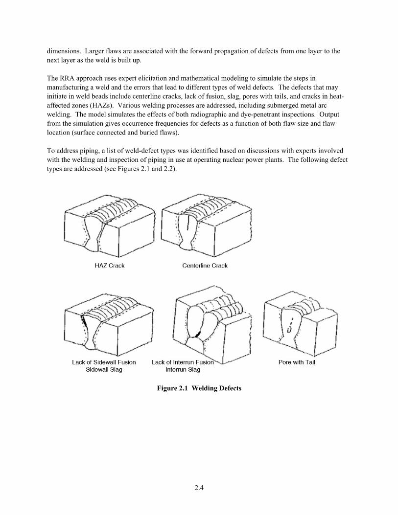
dimensions. Larger flaws are associated with the forward propagation of defects from one layer to the next layer as the weld is built up. The RRA approach uses expert elicitation and mathematical modeling to simulate the steps in manufacturing a weld and the errors that lead to different types of weld defects. The defects that may initiate in weld beads include centerline cracks, lack of fusion, slag, pores with tails, and cracks in heat-affected zones (HAZs). Various welding processes are addressed, including submerged metal arc welding. The model simulates the effects of both radiographic and dye-penetrant inspections. Output from the simulation gives occurrence frequencies for defects as a function of both flaw size and flaw location (surface connected and buried flaws). To address piping, a list of weld-defect types was identified based on discussions with experts involved with the welding and inspection of piping in use at operating nuclear power plants. The following defect types are addressed (see Figures 2.1 and 2.2).
Figure 2.1 Welding Defects
2.4
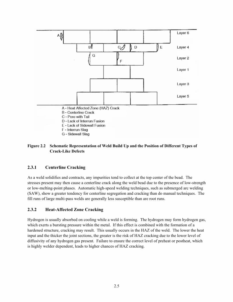
Figure 2.2 Schematic Representation of Weld Build Up and the Position of Different Types of
Crack-Like Defects 2.3.1 Centerline Cracking
As a w solidifies and contracts, any impurield ties tend to collect at the top center of the bead. The stresses present may then cause a centerline crack along the weld bead due to the presence of low-strength
elding The
eat
at or postheat, which highly welder dependent, leads to higher chances of HAZ cracking.
or low-melting-point phases. Automatic high-speed welding techniques, such as submerged arc w(SAW), show a greater tendency for centerline segregation and cracking than do manual techniques. fill runs of large multi-pass welds are generally less susceptible than are root runs. 2.3.2 Heat-Affected Zone Cracking
Hydrogen is usually absorbed on cooling while a weld is forming. The hydrogen may form hydrogen gas, which exerts a bursting pressure within the metal. If this effect is combined with the formation of a hardened structure, cracking may result. This usually occurs in the HAZ of the weld. The lower the hinput and the thicker the joint sections, the greater is the risk of HAZ cracking due to the lower level of diffusivity of any hydrogen gas present. Failure to ensure the correct level of preheis
2.5
2.3.3 Lack of Fusion
The lack-of-fusion defect results from a lack of union between the weld metal and the parent plate or (in multi-run welds) between successive weld runs. The narrower the weld preparation and/or the deepergroove, the greater is the chance of lack of fusion in the weld root. There is a greater chance of lack of sidewall fusion for thicker sections as compared to thinner sections. Occurrence rates for lack-of-fusion defects do not depend on the material type being welded. Any access difficulty preventing the usecorrect electrode angle will increase the chances of lack of fusion. Welder skill is vital in helping to ensure sufficient fu
the
of the
sion when using manual procedures.
ag Inclusions
A)
prone to slag on and the icker the joint, the greater is the likelihood of entrapped inclusions. A dirty base material or oxidized
surfaces will lead ater likelihood of ions. Shop welds are less prone to slag defects than are welds produced in the field nd environment are significant factors since the removal of slag between runs is importa 2.3.5 Porosity
A welded joint will usually contain gas-for phases as the temperature decreases and result in formation of cavitie ormly along the weld. It may be caused b st, or grease surface, oxygen or nitrogen contamination from the atmosphere, or oxygen contamination f lding gas. When porosity occurs in isolated groups, its most likely cause is the existence of unstable conditions as the arc is being struck. Weld metal may be deposited before the gas shield is established. Isolated porosity, which is strung out, is more likely to be caused by incorrect electrode a rikeout. Interdendritic porosity or shrinkage porosity may occur at weld stop-start positions and e linked with solidification cracking. Fluxed processes, such as submerge MA welding, a fluxless processes. Cleanliness is extre mportant. Damp nsumables are a frequent cause of porosity. 2.3.6 Defect Density
Welding metallurgists and inspection engineers estimated the defect occurrence frequencies (per unit length of weld bead) for the set of “crack-like defect types” of the RRA flaw-simulation model. The RRA has not yet published this information lds, which is encoded into the expert system computer code, o se placed it into . However, the methodologies for piping and vessel welds are known to be very similar a nalogous parameters for vessel welds have been published (Chapman et al. 1996; Chapman and Simonen 1998). Table 2.1 indicates the various factors
2.3.4 Non-Metallic Sl
Linear slag inclusions are normally due to incomplete slag removal between weld runs, but slag laminations within the parent plate may occasionally be the cause. Mill scale, rust on the plate, and damaged electrode coatings can cause isolated slag inclusions. Damaged electrode coatings denude theweld metal of slag-forming elements of adequate floatability; i.e., slag is left within the weld bead rather than floating to the top for removal. Slag inclusions are relatively common in manual metal arc (MMand submerged arc weld deposits. Any process resulting in an extremely concave weld bead will be
entrapment between welding runs. The tighter or more narrow the weld preparatith
to a gre nonmetallic inclus. Welder skill ant in avoiding non-metallic inclusions.
ming elements; these evolve intos or porosity. Porosity occurs unif
y moisture, ru on the platerom the shie
ngle or stmay b
d arc or Mmely i
re less susceptible to porosity than workpieces or co or contaminated
for piping wer otherwi the public domain
nd the a
2.6
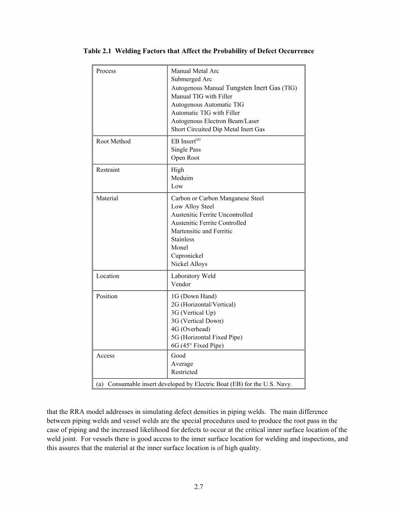
Table 2.1 Welding Factors that Affect the Probability of Defect Occurrence
Process
n Inert Gas (TIG)
TIG atic TIG with Filler
us Electron Beam/Laser ited Dip Metal Inert Gas
Manual Metal ArcSubmerged Arc Autogenous Manual TungsteManual TIG with Filler Autogenous Automatic AutomAutogenoShort Circu
Root Method EB Insert(a) Single Pass Open Root
Restraint High Meduim Low
Material Carbon or Carbon Manganese Steel Low Alloy Steel Austenitic Ferrite Uncontrolled
Monel Cupronickel Nickel Alloys
Austenitic Ferrite Controlled Martensitic and Ferritic Stainless
Location Laboratory Weld Vendor
Position 1G (Down Hand) 2G (Horizontal/Vertical) 3G (Vertical Up) 3G (Vertical Down) 4G (Overhead) 5G (Horizontal Fixed Pipe) 6G (45° Fixed Pipe)
Access Good Average Restricted
(a) Consumable insert developed by Electric Boat (EB) for the U.S. Navy. that the RRA model addresses in simulating defect densities in piping welds. The main difference
etween piping welds and vessel welds are the special procedures used to produce the root pass in the
bcase of piping and the increased likelihood for defects to occur at the critical inner surface location of the weld joint. For vessels there is good access to the inner surface location for welding and inspections, andthis assures that the material at the inner surface location is of high quality.
2.7
As indicated in Table 2.1, the model explicitly accounts for the expected increases in defect occrates for welding at f
urrence ield and vendor sites. The model also addresses difficult field welding conditions as
ey may be related to access to the weld (e.g., restricted access) and to the welding position (e.g., 4G
he Chapman (1993) model allows the expected number of each type of defect to be calculated, and also
s
effects of inspections. The weld-simulation model assigns defect locations within the pipe all and identifies flaws that are surface connected with the assumption that defects occur randomly
ake up the completed weld.
he next question was the probability that a defect, once initiated, would propagate on to the next layer or
he
Simonen 1998).
her are combined into a ingle larger defect. In general, the likelihood of flaw interaction is relatively low. The flaws that
imary contributor to the simulated population of larger flaws.
he data encoded within the expert system model describe the defects generated by the welding process. oth
he plemented methods for calculating inspection efficiency
thOverhead welding). 2.3.7 Defect Characteristics
Tdefines the various characteristics (e.g., size, location, etc.) of these defects. The defect parameters for piping welds are defect width, defect depth, length-to-depth ratio, defect angle, and probability of forwardpropagation. Through-wall and length dimensions are quantified for purposes of fracture mechaniccalculations. The angle and separation between the surfaces of the defects are evaluated for purposes of simulating thewwithin the individual runs that m
Experts believed that the sizes of the individual defects as they first initiate within a single weld run could be realistically estimated. The bead dimension served as a normalizing factor for the sizes of these initiated defects, although their sizes were not always truncated at the bead depth. A Weibull statistical distribution was selected to describe the depth dimensions of the initiated defects. The experts also estimated defect lengths that could be described by Weibull distributions for flaw-aspect ratios that related the lengths of the flaws to the corresponding flaw-depth dimensions. Tadditional layers of the weld. The model was therefore designed to predict the number of small defects initiated in the welding process that would grow to become larger defects before the weld was completed. The ability of the welder to observe and correct the errors was also considered for each type of propagating defect. Probabilities to quantify the statistical distributions are encoded into the RRA expert system model. Tprobabilities for initial defect characteristics and for the propagation of these defects for piping welds have not yet been published, but are believed to be similar to those for the RRA model for vessel welds (Chapman et al. 1996; Chapman and Interactions between the randomly located defects in a weld are also simulated using a flaw proximity rule described by Chapman (1993). One or more defects sufficiently close togetspropagate from layer to layer during welding are the pr
2.3.8 Inspection Model
TA second aspect of the model simulates the effects of the inspections that are performed in the shop bduring and after the welding process is completed. The present report does not document details of tinspection models. The RRA model has im
2.8
2.9
urves for each type of defect in the weld of interest, with the inspection efficiency being a function of the
a slot ta and experience of
spectors were used to convert calculated images to probabilities of detection. Inputs to the simulation d
he defect width or separation between efect surfaces can be relatively large for welding defects as compared to the widths of typical service-
-type defects.
encies for given defect lengths and widths were based on e whether as welded or machined.
onte Carlo simulation procedure. A computer code (RR-PRODIGAL) has been written for application on a UNIX-based workstation with the parameters for the specific welds defined through interactive menu-driven inputs. A weld is described as a series of activities. One type of activity consists of the stepwise process of constructing the weld as a series of weld beads and layers as a set of building blocks as indicated in Figure 2.2. Other activities are as follows. Inspections. Either radiographic or surface inspections can be performed at any stage, either during the partial weld buildup or after all weld runs have been completed. It is assumed that all detected defects are repaired, and these defects are not counted as contributions to the simulated population of defects. Comparisons (Chapman and Simonen 1998) of the model predictions with data from vessel welds indicate that improved correlations should consider that governing repair criterion. Machining. Post-weld machining is considered a factor that affects the surface finish, which in turn impacts the effectiveness of surface inspections. Machining can also expose near-surface buried defects and thereby increase the number of surface-breaking defects. Post Weld Heat Treatment. The sizes of HAZ cracks can be extended by simulating the effects of post-weld heat treatment. 2.5 Inputs for Sensitivity Study
RRA, under a subcontract arrangement with PNNL, used the RR-PRODIGAL computer code to perform a set of sensitivity calculations. These calculations studied the effects of various welding and inspection parameters on the predicted numbers and sizes of flaws in representative nuclear-piping welds. Table 2.2 lists the parameters for the sensitivity calculations.
cdefect size and its through-wall location. Both radiographic and surface (dye penetrant) inspection methods are addressed. Radiography is simulated using the model of Halmshaw and Hunt (1975). Each defect is treated asthat produces a difference in image density that the inspector must interpret. Test dainmodel define details of the radiographic procedure, including specifying the isotope or x-ray source anfilm location. Image densities are predicted based on the defect location relative to the source and film, and the defect size, width, and angle. It should be noted that tdinduced cracks such, as fatigue cracks. As a result, the radiography inspections can be relatively effective for the larger welding For surface examinations, the inspection efficijudgm nts with consideration of surface finish 2.4 Computer-Based Implementation
The expert system model of weld buildup uses a M
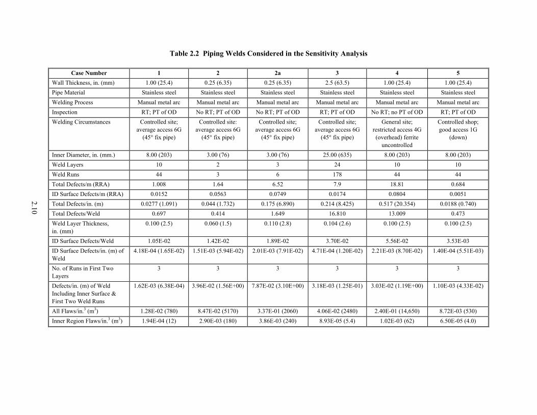
Table 2.2 Piping Welds Considered in the Sensitivity Analysis
2.10
Case Number 1 2 2a 3 4 5
Wall Thickness, in. (mm) 1.00 (25.4) 0.25 (6.35) 0.25 (6.35) 2.5 (63.5) 1.00 (25.4) 1.00 (25.4) Pipe Material Stainless steel Stainless steel Stainless steel Stainless steel Stainless steel Stainless steel Welding Process Manual metal arc Manual metal arc Manual metal arc Manual metal arc Manual metal arc Manual metal arc Inspection RT; PT of OD No RT; PT of OD No RT; PT of OD RT; PT of OD No RT; no PT of OD RT; PT of OD Welding Circumstances Controlled site;
average access 6G (45° fix pipe)
Controlled site: average access 6G
(45° fix pipe)
Controlled site; average access 6G
(45° fix pipe)
Controlled site; average access 6G
(45° fix pipe)
General site; restricted access 4G (overhead) ferrite
uncontrolled
Controlled shop; good access 1G
(down)
Inner Diameter, in. (mm.) 8.00 (203) 3.00 (76) 3.00 (76) 25.00 (635) 8.00 (203) 8.00 (203) Weld Layers 10 2 3 24 10 10 Weld Runs 44 3 6 178 44 44 Total Defects/m (RRA) 1.008 1.64 6.52 7.9 18.81 0.684ID Surface Defects/m (RRA) 0.0152 0.0563 0.0749 0.0174 0.0804 0.0051Total Defects/in. (m) 0.0277 (1.091) 0.044 (1.732) 0.175 (6.890) 0.214 (8.425) 0.517 (20.354) 0.0188 (0.740) Total Defects/Weld 0.697 0.414 1.649 16.810 13.009 0.473Weld Layer Thickness, in. (mm)
0.100 (2.5) 0.060 (1.5) 0.110 (2.8) 0.104 (2.6) 0.100 (2.5) 0.100 (2.5)
ID Surface Defects/Weld 1.05E-02 1.42E-02 1.89E-02 3.70E-02 5.56E-02 3.53E-03ID Surface Defects/in. (m) of Weld
4.18E-04 (1.65E-02) 1.51E-03 (5.94E-02) 2.01E-03 (7.91E-02) 4.71E-04 (1.20E-02) 2.21E-03 (8.70E-02) 1.40E-04 (5.51E-03)
No. of Runs in First Two Layers
3 3 3 3 3 3
Defects/in. (m) of Weld Including Inner Surface & First Two Weld Runs
1.62E-03 (6.38E-04) 3.96E-02 (1.56E+00) 7.87E-02 (3.10E+00) 3.18E-03 (1.25E-01) 3.03E-02 (1.19E+00) 1.10E-03 (4.33E-02)
All Flaws/in.3 (m3) 1.28E-02 (780) 8.47E-02 (5170) 3.37E-01 (2060) 4.06E-02 (2480) 2.40E-01 (14,650) 8.72E-03 (530) Inner Region Flaws/in.3 (m3) 1.94E-04 (12) 2.90E-03 (180) 3.86E-03 (240) 8.93E-05 (5.4) 1.02E-03 (62) 6.50E-05 (4.0)
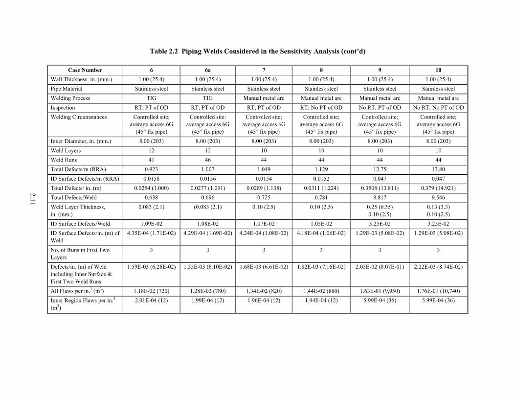
Table 2.2 Piping Welds Considered in the Sensitivity Analysis (cont’d)
2.11
Case Number 6 6a 7 8 9 10
Wall Thickness, in. (mm.) 1.00 (25.4) 1.00 (25.4) 1.00 (25.4) 1.00 (25.4) 1.00 (25.4) 1.00 (25.4) Pipe Material Stainless steel Stainless steel Stainless steel Stainless steel Stainless steel Stainless steel Welding Process TIG TIG Manual metal arc Manual metal arc Manual metal arc Manual metal arc Inspection RT; PT of OD RT; PT of OD RT; PT of OD RT; No PT of OD No RT; PT of OD No RT; No PT of OD Welding Circumstances Controlled site;
average access 6G (45° fix pipe)
Controlled site: average access 6G
(45° fix pipe)
Controlled site; average access 6G
(45° fix pipe)
Controlled site; average access 6G
(45° fix pipe)
Controlled site; average access 6G
(45° fix pipe)
Controlled site; average access 6G
(45° fix pipe) Inner Diameter, in. (mm.) 8.00 (203) 8.00 (203) 8.00 (203) 8.00 (203) 8.00 (203) 8.00 (203) Weld Layers 12 12 10 10 10 10Weld Runs 41 46 44 44 44 44Total Defects/m (RRA) 0.923 1.007 1.049 1.129 12.75 13.80ID Surface Defects/m (RRA) 0.0158 0.0156 0.0154 0.0152 0.047 0.047Total Defects/ in. (m) 0.0254 (1.000) 0.0277 (1.091) 0.0289 (1.138) 0.0311 (1.224) 0.3508 (13.811) 0.379 (14.921) Total Defects/Weld 0.638 0.696 0.725 0.781 8.817 9.546Weld Layer Thickness, in. (mm.)
0.083 (2.1) (0.083 (2.1) 0.10 (2.5) 0.10 (2.5) 0.25 (6.35) 0.10 (2.5)
0.13 (3.3) 0.10 (2.5)
ID Surface Defects/Weld 1.09E-02 1.08E-02 1.07E-02 1.05E-02 3.25E-02 3.25E-02ID Surface Defects/in. (m) of Weld
4.35E-04 (1.71E-02) 4.29E-04 (1.69E-02) 4.24E-04 (1.08E-02) 4.18E-04 (1.06E-02) 1.29E-03 (5.08E-02) 1.29E-03 (5.08E-02)
No. of Runs in First Two Layers
3 3 3 3 3 3
Defects/in. (m) of Weld including Inner Surface & First Two Weld Runs
1.59E-03 (6.26E-02) 1.55E-03 (6.10E-02) 1.68E-03 (6.61E-02) 1.82E-03 (7.16E-02) 2.05E-02 (8.07E-01) 2.22E-03 (8.74E-02)
All Flaws per in.3 (m3) 1.18E-02 (720) 1.28E-02 (780) 1.34E-02 (820) 1.44E-02 (880) 1.63E-01 (9,950) 1.76E-01 (10,740) Inner Region Flaws per in.3 (m3)
2.01E-04 (12) 1.99E-04 (12) 1.96E-04 (12) 1.94E-04 (12) 5.99E-04 (36) 5.99E-04 (36)
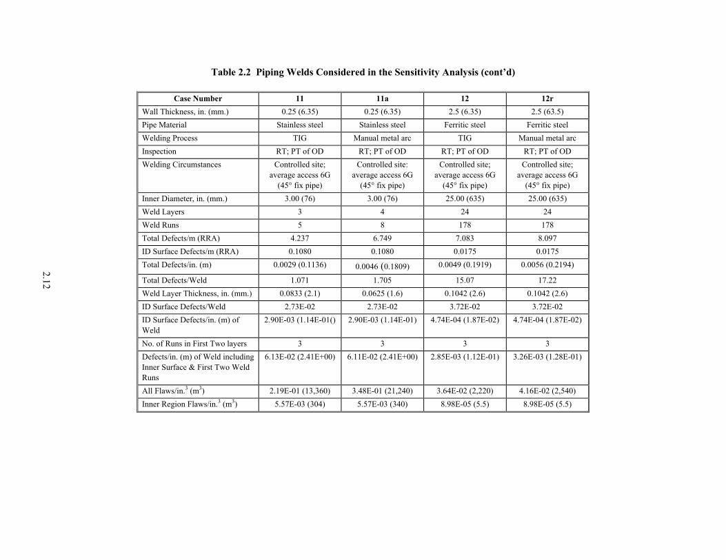
Case Number 11 11a 12 12r Wall Thickness, in. (mm.) 0.25 (6.35) 0.25 (6.35) 2.5 (6.35) 2.5 (63.5) Pipe Material Stainless steel Stainless steel Ferritic steel Ferritic steel Welding Process TIG Manual metal arc TIG Manual metal arc Inspection RT; PT of OD RT; PT of OD RT; PT of OD RT; PT of OD Welding Circumstances Controlled site;
average access 6G (45° fix pipe)
Controlled site: average access 6G
(45° fix pipe)
Controlled site; average access 6G
(45° fix pipe)
Controlled site; average access 6G
(45° fix pipe) Inner Diameter, in. (mm.) 3.00 (76) 3.00 (76) 25.00 (635) 25.00 (635) Weld Layers 3 4 24 24 Weld Runs 5 8 178 178 Total Defects/m (RRA) 4.237 6.749 7.083 8.097ID Surface Defects/m (RRA) 0.1080 0.1080 0.0175 0.0175 Total Defects/in. (m) 0.0029 (0.1136) 0.0046 (0.1809) 0.0049 (0.1919) 0.0056 (0.2194)
Total Defects/Weld 1.071 1.705 15.07 17.22Weld Layer Thickness, in. (mm.) 0.0833 (2.1) 0.0625 (1.6) 0.1042 (2.6) 0.1042 (2.6)ID Surface Defects/Weld 2.73E-02 2.73E-02 3.72E-02 3.72E-02ID Surface Defects/in. (m) of Weld
2.90E-03 (1.14E-01() 2.90E-03 (1.14E-01) 4.74E-04 (1.87E-02) 4.74E-04 (1.87E-02)
No. of Runs in First Two layers 3 3 3 3 Defects/in. (m) of Weld including Inner Surface & First Two Weld Runs
6.13E-02 (2.41E+00) 6.11E-02 (2.41E+00) 2.85E-03 (1.12E-01) 3.26E-03 (1.28E-01)
All Flaws/in.3 (m3) 2.19E-01 (13,360) 3.48E-01 (21,240) 3.64E-02 (2,220) 4.16E-02 (2,540) Inner Region Flaws/in.3 (m3) 5.57E-03 (304) 5.57E-03 (340) 8.98E-05 (5.5) 8.98E-05 (5.5)
Table 2.2 Piping Welds Considered in the Sensitivity Analysis (cont’d)
2.12
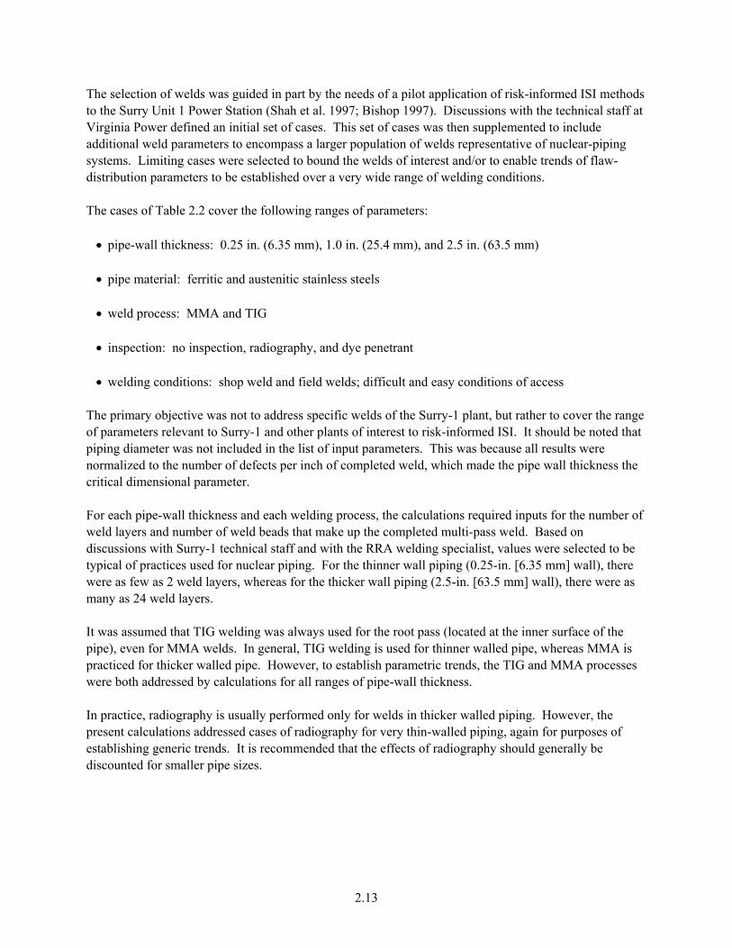
The selection of welds was guided in part by the needs of a pilot application of risk-informed ISI methods to the Surry Unit 1 Power Station (Shah et al. 1997; Bishop 1997). Discussions with the technical staff at Virginia Power defined an initial set of cases. This set of cases was then supplemented to include additional weld parameters to encompass a larger population of welds representative of nuclear-piping systems. Limiting cases were selected to bound the welds of interest and/or to enable trends of flaw-distribution parameters to be established over a very wide range of welding conditions. The cases of Table 2.2 cover the following ranges of parameters: • pipe-wall thickness: 0.25 in. (6.35 mm), 1.0 in. (25.4 mm), and 2.5 in. (63.5 mm)
• pipe material: ferritic and austenitic stainless steels
• weld process: MMA and TIG
• inspection: no inspection, radiography, and dye penetrant
• welding conditions: shop weld and field welds; difficult and easy conditions of access
The primary objective was not to address specific welds of the Surry-1 plant, but rather to cover the range of parameters relevant to Surry-1 and other plants of interest to risk-informed ISI. It should be noted that piping diameter was not included in the list of input parameters. This was because all results were normalized to the number of defects per inch of completed weld, which made the pipe wall thickness the critical dimensional parameter. For each pipe-wall thickness and each welding process, the calculations required inputs for the number of weld layers and number of weld beads that make up the completed multi-pass weld. Based on discussions with Surry-1 technical staff and with the RRA welding specialist, values were selected to be typical of practices used for nuclear piping. For the thinner wall piping (0.25-in. [6.35 mm] wall), there were as few as 2 weld layers, whereas for the thicker wall piping (2.5-in. [63.5 mm] wall), there were as many as 24 weld layers. It was assumed that TIG welding was always used for the root pass (located at the inner surface of the pipe), even for MMA welds. In general, TIG welding is used for thinner walled pipe, whereas MMA is practiced for thicker walled pipe. However, to establish parametric trends, the TIG and MMA processes were both addressed by calculations for all ranges of pipe-wall thickness. In practice, radiography is usually performed only for welds in thicker walled piping. However, the present calculations addressed cases of radiography for very thin-walled piping, again for purposes of establishing generic trends. It is recommended that the effects of radiography should generally be discounted for smaller pipe sizes.
2.13
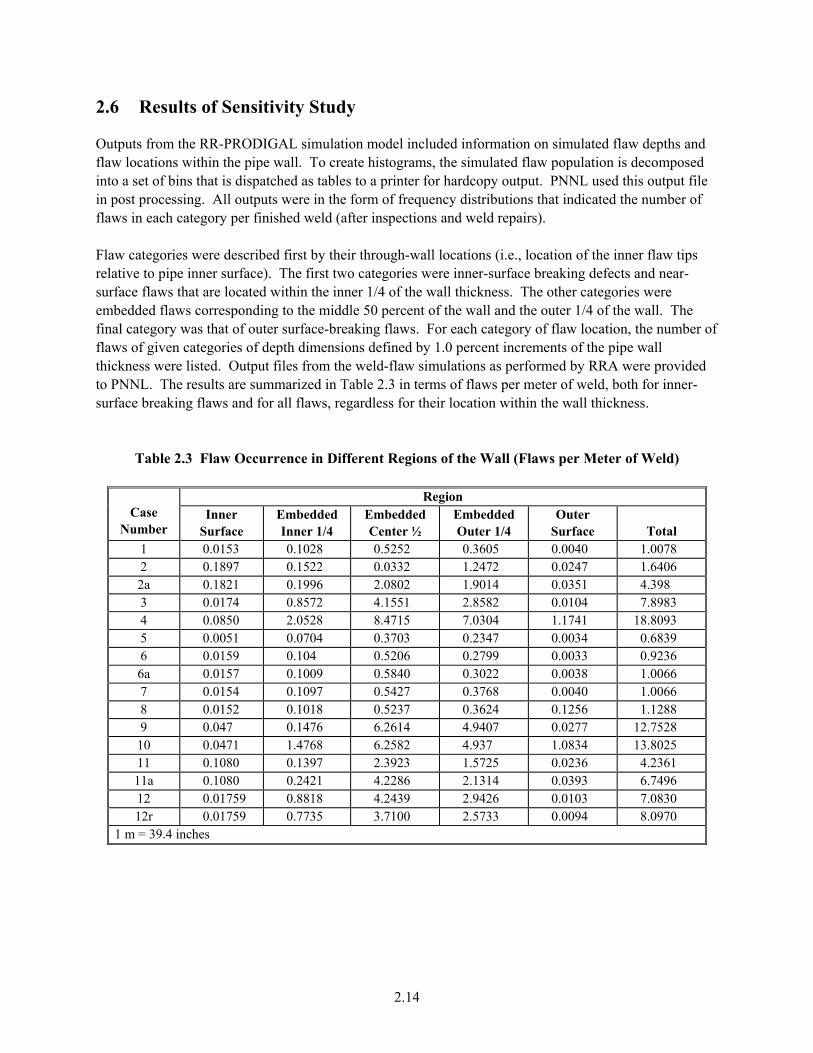
2.6 Results of Sensitivity Study
Outputs from the RR-PRODIGAL simulation model included information on simulated flaw depths and flaw locations within the pipe wall. To create histograms, the simulated flaw population is decomposed into a set of bins that is dispatched as tables to a printer for hardcopy output. PNNL used this output file in post processing. All outputs were in the form of frequency distributions that indicated the number of flaws in each category per finished weld (after inspections and weld repairs). Flaw categories were described first by their through-wall locations (i.e., location of the inner flaw tips relative to pipe inner surface). The first two categories were inner-surface breaking defects and near-surface flaws that are located within the inner 1/4 of the wall thickness. The other categories were embedded flaws corresponding to the middle 50 percent of the wall and the outer 1/4 of the wall. The final category was that of outer surface-breaking flaws. For each category of flaw location, the number of flaws of given categories of depth dimensions defined by 1.0 percent increments of the pipe wall thickness were listed. Output files from the weld-flaw simulations as performed by RRA were provided to PNNL. The results are summarized in Table 2.3 in terms of flaws per meter of weld, both for inner-surface breaking flaws and for all flaws, regardless for their location within the wall thickness.
Table 2.3 Flaw Occurrence in Different Regions of the Wall (Flaws per Meter of Weld)
Region Case
Number Inner
Surface Embedded Inner 1/4
Embedded Center ½
Embedded Outer 1/4
Outer Surface Total
1 0.0153 0.1028 0.5252 0.3605 0.0040 1.0078 2 0.1897 0.1522 0.0332 1.2472 0.0247 1.6406 2a 0.1821 0.1996 2.0802 1.9014 0.0351 4.398 3 0.0174 0.8572 4.1551 2.8582 0.0104 7.8983 4 0.0850 2.0528 8.4715 7.0304 1.1741 18.8093 5 0.0051 0.0704 0.3703 0.2347 0.0034 0.6839 6 0.0159 0.104 0.5206 0.2799 0.0033 0.9236 6a 0.0157 0.1009 0.5840 0.3022 0.0038 1.0066 7 0.0154 0.1097 0.5427 0.3768 0.0040 1.0066 8 0.0152 0.1018 0.5237 0.3624 0.1256 1.1288 9 0.047 0.1476 6.2614 4.9407 0.0277 12.7528
10 0.0471 1.4768 6.2582 4.937 1.0834 13.8025 11 0.1080 0.1397 2.3923 1.5725 0.0236 4.2361 11a 0.1080 0.2421 4.2286 2.1314 0.0393 6.7496 12 0.01759 0.8818 4.2439 2.9426 0.0103 7.0830 12r 0.01759 0.7735 3.7100 2.5733 0.0094 8.0970
1 m = 39.4 inches
2.14
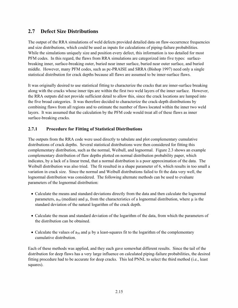
2.7 Defect Size Distributions
The output of the RRA simulations of weld defects provided detailed data on flaw-occurrence frequencies and size distributions, which could be used as inputs for calculations of piping-failure probabilities. While the simulations uniquely size and position every defect, this information is too detailed for most PFM codes. In this regard, the flaws from RRA simulations are categorized into five types: surface-breaking inner, surface-breaking outer, buried near inner surface, buried near outer surface, and buried middle. However, many PFM codes, such as pc-PRAISE and SRRA (Bishop 1997) need only a single statistical distribution for crack depths because all flaws are assumed to be inner-surface flaws. It was originally desired to use statistical fitting to characterize the cracks that are inner-surface breaking along with the cracks whose inner tips are within the first two weld layers of the inner surface. However, the RRA outputs did not provide sufficient detail to allow this, since the crack locations are lumped into the five broad categories. It was therefore decided to characterize the crack-depth distributions by combining flaws from all regions and to estimate the number of flaws located within the inner two weld layers. It was assumed that the calculation by the PFM code would treat all of these flaws as inner surface-breaking cracks. 2.7.1 Procedure for Fitting of Statistical Distributions
The outputs from the RRA code were used directly to tabulate and plot complementary cumulative distributions of crack depths. Several statistical distributions were then considered for fitting this complementary distribution, such as the normal, Weibull, and lognormal. Figure 2.3 shows an example complementary distribution of flaw depths plotted on normal distribution probability paper, which indicates, by a lack of a linear trend, that a normal distribution is a poor approximation of the data. The Weibull distribution was also tried. The fit resulted in a shape parameter of 6, which results in too small a variation in crack size. Since the normal and Weibull distributions failed to fit the data very well, the lognormal distribution was considered. The following alternate methods can be used to evaluate parameters of the lognormal distribution: • Calculate the means and standard deviations directly from the data and then calculate the lognormal
parameters, a50 (median) and µ, from the characteristics of a lognormal distribution, where µ is the standard deviation of the natural logarithm of the crack depth.
• Calculate the mean and standard deviation of the logarithm of the data, from which the parameters of
the distribution can be obtained. • Calculate the values of a50 and µ by a least-squares fit to the logarithm of the complementary
cumulative distribution. Each of these methods was applied, and they each gave somewhat different results. Since the tail of the distribution for deep flaws has a very large influence on calculated piping-failure probabilities, the desired fitting procedure had to be accurate for deep cracks. This led PNNL to select the third method (i.e., least squares).
2.15
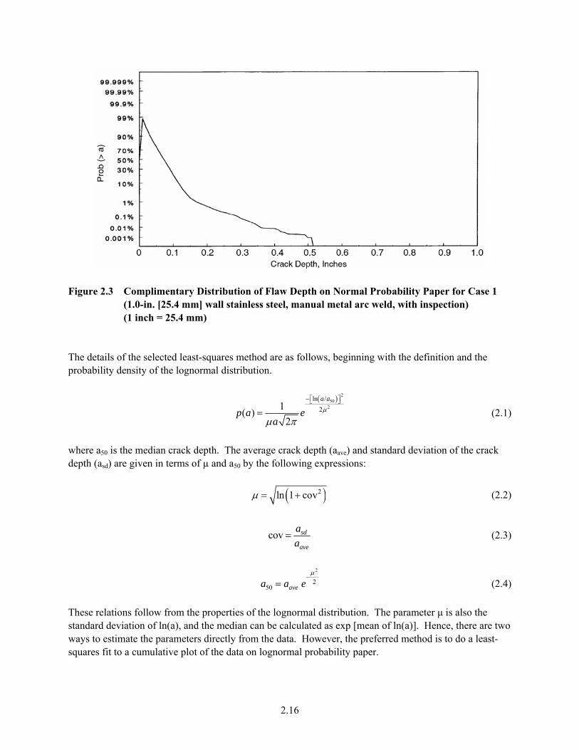
F epth on Normal Probability Paper for Case 1 igure 2.3 Complimentary Distribution of Flaw D
(1.0-in. [25.4 mm] wall stainless steel, manual metal arc weld, with inspection) (1 inch = 25.4 mm)
he details of the selected least-squares method are asrobability density of the lognormal distribution.
T follows, beginning with the definition and the p
( ) 2
502
ln /21( )
2
a a
p a ea
µ
µ π
−⎡ ⎤⎣ ⎦
= (2.1)
where a50 is the median crack depth. The average crack depth (aave) and standard deviation of the crackdepth (asd) are given in terms of µ and a50 by the following expressions:
( )2ln 1 covµ = + (2
.2)
cov sda= (2.3)
avea
2
250 avea a e
µ−
= (2.4) These relations follow from the properties of the lognormal distribution. The parameter µ is also the tandard deviation of ln(a), and the median can be calculated as exp [mean of
ways to estimate the parameters directly from the data. However, the preferred method is to do a least-squares fit to a cumulative plot of the data on lognormal probability paper.
s ln(a)]. Hence, there are two
2.16

Before selecting the least-squares approach as the preferred method, the parameters of the log-normal distribution were calculated using, as possible alternatives, the method of moments and the maximum-likelihood method, along with the least-squares-fit method. The parameters obtained using the maximum-likelihood method provided a poor fit to the data. The method of moments consistently
d a thod and gave a better fit than the maximum-likelihood method. The method of moments gives equal weight to each data point. It provided
provide lower shape parameter than the maximum-likelihood me
undesirably high probabilities in the upper tail of the data. Therefore, the least-squares method was usedto solve the following: Find µ and a50 such that
21 1 a⎧ ⎫⎛ ⎞⎡ ⎤
[ ]
10050
1
2 2log minimum
0actuali
aPµ
=
⎪ ⎪lnerfc⎪ ⎪⎜ ⎟⎢ ⎥
⎜ ⎟⎣ ⎦ =⎨ ⎬⎜ ⎟>⎪ ⎪⎜ ⎟⎪ ⎪⎜ ⎟
⎝ ⎠
(2.5)
ain the global minimum. In practice, es of µ and a50 used for the numerical um values to the above functions.
of
ns and the finite number putation. Figure 2.4 also provides fitting results that were obtained
using the least-square procedure. The fit is relatively he lack of smoothness of the data. The
he complementarypresentative cases are shown in the plots of Figures 2.4 through 2.9. The results of the data fitting are mmarized in Table 2.4. This table lists the pipe-wall thickness, the inner pipe diameter, the weld-layer
thickness, and the mean, the standard deviation, the median, and the shape parameter of flaw-depth distribution for all cases addressed by the RRA calculations. 2.7.3 Effects of Weld Process on Depth Distribution
Figure 2.10 addresses the wall thickness of 1 in. (25.4 mm), and compares results for the baseline Case #1 (stainless steel MMA weld with inspection) with other results obtained by taking variations for the welding parameters relative to those of the baseline case. The depth distributions are relatively insensitive to the welding parameters for small flaws, but become increasingly sensitive to welding parameters as the flaw depths become larger. The following trends are evident:
⎩ ⎭
∑
he idea in the least-square method is to minimize the error and obtT
the results appeared to be sensitive to the choice of the initial valusearch process, which indicated that there are several local minim 2.7.2 Resulting Lognormal Flaw-Depth Distributions
The outputs from the RRA code were first used directly to determine the complementary distributioncrack depths. Figure 2.4 was obtained by summing up the contents of the bins in the output tables for
ase 1. This data distribution is not smooth, which is due to modeling assumptioCof Monte Carlo trails used in the com
good given tparameters of the distribution are shown in the upper right corner of the plot.
distribution of the raw data and the lognormal distribution fit for several Tresu
2.17
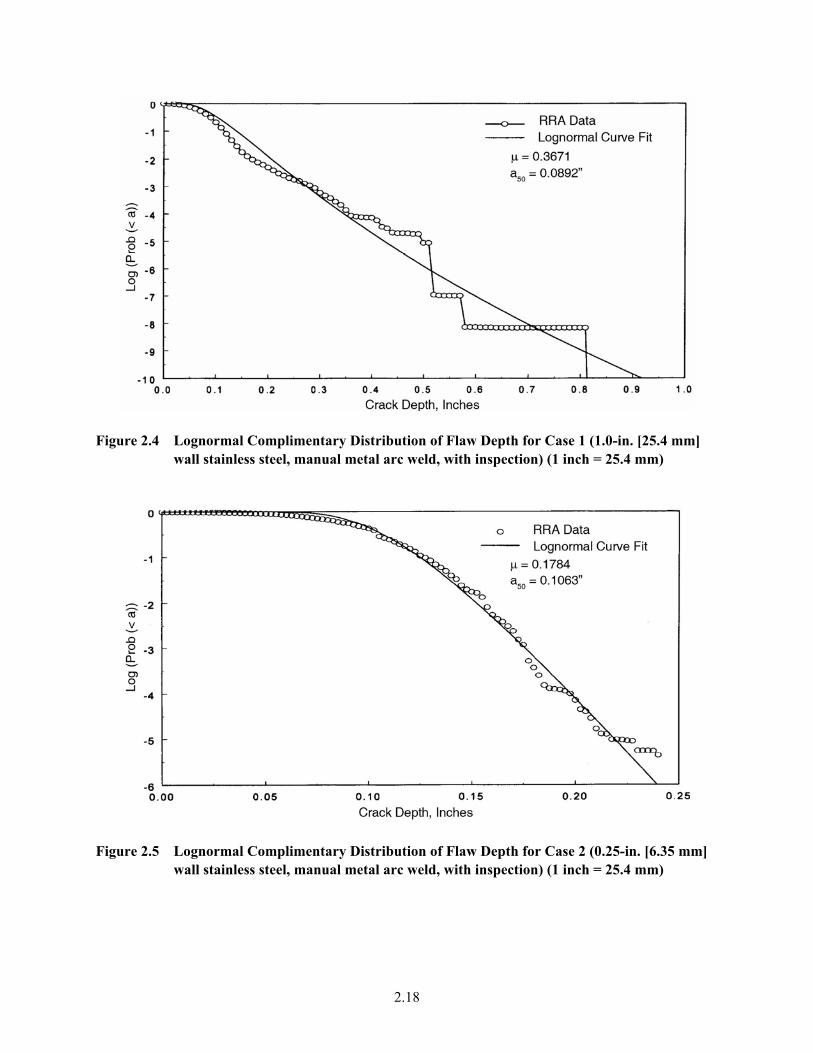
Figure 2.4 Lognormal Complimentary Distribution of Flaw Depth for Case 1 (1.0-in. [25.4 mm] wall stainless steel, manual metal arc weld, with inspection) (1 inch = 25.4 mm)
Figure 2.5 Lognormal Complimentary Distribution of Flaw Depth for Case 2 (0.25-in. [6.35 mm]
wall stainless steel, manual metal arc weld, with inspection) (1 inch = 25.4 mm)
2.18
Figure 2.6 Lognormal Complimentary Distribution of Flaw Depth for Case 3 (2.5-in. [63.5 mm] wall stainless steel, manual metal arc weld, with inspection) (1 inch = 25.4 mm)
Figure 2.7 Lognormal Complimentary Distribution of Flaw Depth for Case 6 (1.0-in. [25.4 mm]
wall stainless steel, tungsten inert gas weld, with inspection) (1 inch = 25.4 mm)
2.19
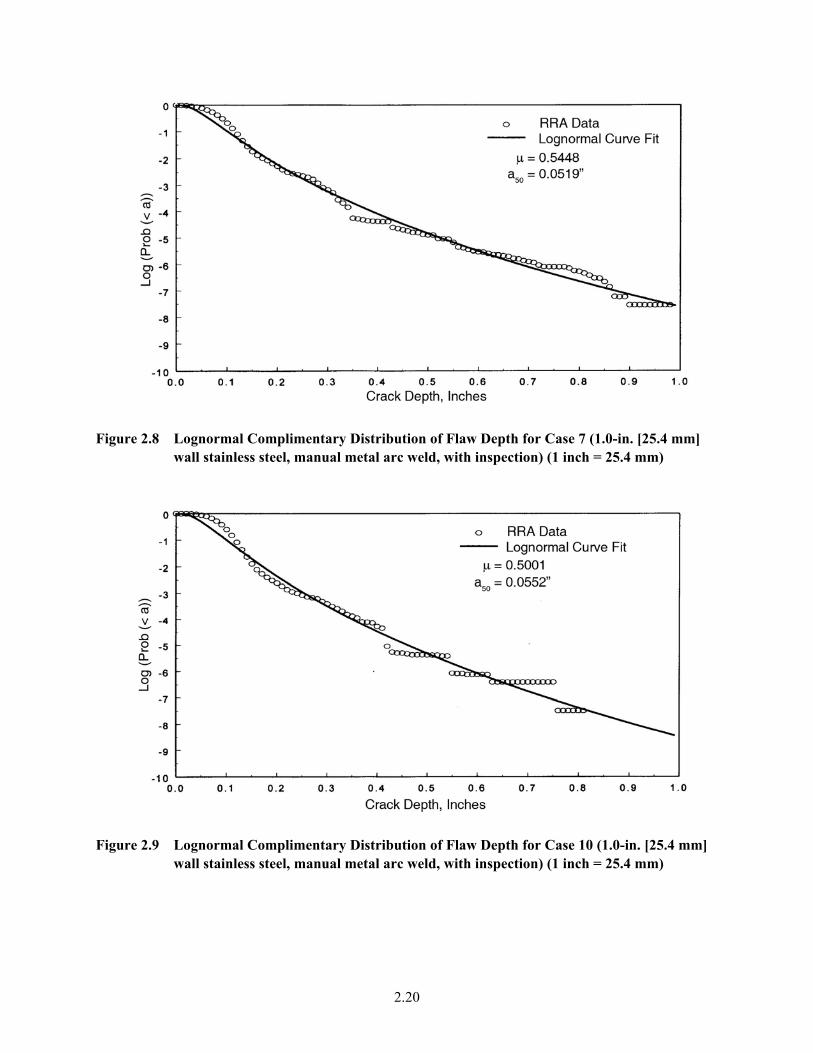
Figure 2.8 Lognormal Complimentary Distribution of Flaw Depth for Case 7 (1.0-in. [25.4 mm]
wall stainless steel, manual metal arc weld, with inspection) (1 inch = 25.4 mm)
Figure 2.9 Lognormal Complimentary Distribution of Flaw Depth for Case 10 (1.0-in. [25.4 mm]
wall stainless steel, manual metal arc weld, with inspection) (1 inch = 25.4 mm)
2.20

Table 2.4 Summary of Distribution Parameters
Case Number
Wall Thickness, in. (mm)
Inner Diameter, in. (mm)
Weld Layer Thickness, in. (mm)
Mean Flaw Depth,
in. (mm)
Standard Deviation, in. (mm)
Median (a50),
in. (mm)
Shape Parameter
(µ) 1 1.00
(25.4) 8.00 (203)
0.100 (2.54)
0.095 (2.42)
0.036 (0.92)
0.089 (2.26)
0.3671
2 0.25 (6.35)
3.00 (76)
0.125 (3.17)
0.109 (2.77)
0.022 (0.58)
0.106 (2.70)
0.1784
2a 0.25 (6.35)
3.00 (76)
0.083 (2.12)
0.071 (1.82)
0.016 (0.43)
0.069 (1.77)
0.2593
3 2.50 (63.5)
25.0 (635)
0.104 (2.65)
0.062 (1.60)
0.033 (0.85)
0.055 (1.41)
0.4992
4 1.00 (25.4)
8.00 (203)
0.100 (2.54)
0.084 (2.15)
0.035 (0.89)
0.078 (1.99)
0.3977
5 1.00 (25.4)
8.00 (203)
0.100 (2.54)
0.072 (1.85)
0.035 (0.90)
0.065 (1.66)
0.4606
6 1.00 (25.4)
8.00 (203)
0.083 (2.12)
0.085 (2.16)
0.030 (0.76)
0.080 (2.04)
0.3418
6a 1.00 (25.4)
8.00 (203)
0.083 (2.12)
0.081 (2.06)
0.029 (0.74)
0.076 (1.94)
0.3503
7 1.00 (25.4)
8.00 (203)
0.100 (2.54)
0.060 (1.53)
0.035 (0.90)
0.052 (1.32)
0.5448
8 1.00 (25.4)
8.00 (203)
0.100 (2.54)
0.125 (3.20)
0.037 (0.95)
0.052 (1.32)
0.2902
9 1.00 (25.4)
8.00 (203)
0.100 (2.54)
0.114 (2.90)
0.034 (0.88)
0.106 (2.71)
0.3021
10 1.00 (25.4)
8.00 (203)
0.100 (2.54)
0.062 (1.59)
0.033 (0.85)
0.055 (1.40)
0.5001
11 0.25 (6.35)
3.00 (76)
0.083 (2.12)
0.066 (1.70)
0.021 (0.54)
0.063 (1.61)
0.3113
11a 0.25 (6.35)
3.00 (76)
0.062 (1.59)
0.043 (1.10)
0.019 (0.48)
0.039 (1.01)
0.4199
12 2.50 (63.5)
25.0 (635)
0.104 (2.65)
0.045 (1.15)
0.035 (0.90)
0.038 (0.98)
0.6996
12r 2.50 (63.5)
25.0 (635)
0.104 (2.65)
0.027 (0.69)
0.027 (0.71)
0.019 (0.49)
0.8346
2.21

Figure 2.10 Comparison of Simulated Flaw Depth Distributions for 1-in. (25.4 mm) Wall Pipe
Welds (1 inch = 25.4 mm) • Ferritic steel welds have a greater potential than stainless steel welds to have flaws with very large
depths. This trend may be because ferritic steels are susceptible to the mechanism of HAZ cracking.
• Inservice inspections are most effective in reducing the number of very deep flaws with a much smaller effect on reducing the number of shallow flaws.
• TIG welds tend to have fewer flaws of large depths compared to welds made by the MMA welding
process. This effect is due in part to the inherent occurrence rates for flaws from the TIG welding process. In addition, there are typically more weld layers for TIG welds, which creates more opportunities for the arrest of flaws as they grow from layer to layer during the welding.
Figure 2.11 addresses welds made with the same set of process parameters, but for piping of different wall thicknesses, which range from 0.25 to 2.5 in. (6.35 to 63.5 mm). It is seen that there is a greater likelihood for a given flaw to have a larger depth as the pipe-wall thickness becomes greater. It should also be noted that Figure 2.11 addresses only conditional depth distributions with the flaw density not being a factor. Thicker welds in larger diameter piping will have more weld metal, which in turn implies more flaws per weld for larger piping. As a result, the expected number of large flaws per weld will be significantly greater for larger sizes of piping, both from the standpoint of flaw-density considerations and
om the trends of the conditional flaw-depth distribution curves.
imulated dist hs. The flaw depths are shown here as a function of the flaw depth as fraction of the wall thickness (i.e., as a function of a/t) as opposed to Figure 2.11, which gives flaw
While the occurrence rate for this mechanism is relatively small, it has the potential to produce verydeep cracks if the proper conditions are present to cause its occurrence.
fr Figure 2.12 presents a somewhat different perspective on the relationship of pipe-wall thickness to the
ributions of flaw deptsa
2.22
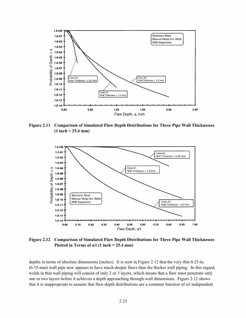
Figure 2.11 Comparison of Simulated Flaw Depth Distributions for Three Pipe Wall Thicknesses
(1 inch = 25.4 mm)
Figure 2.12 Comparison of Simulated Flaw Depth Distributions for Three Pipe Wall Thicknesses
Plotted in Terms of a/t (1 inch = 25.4 mm) depths in terms of absolute dimensions (inches). It is seen in Figure 2.12 that the very thin 0.25-in. (6.35-mm) wall pipe now appears to have much deeper flaws than the thicker wall piping. In this regard, welds in thin wall piping will consist of only 2 or 3 layers, which means that a flaw must penetrate only one or two layers before it achieves a depth approaching through-wall dimensions. Figure 2.12 shows that it is inappropriate to assume that flaw-depth distributions are a common function of a/t independent
2.23
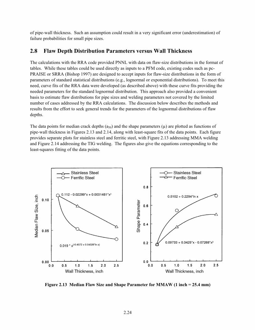
of pipe-wall thickness. Such an assumption could result in a very significant error (underestimation) of failure probabilities for small pipe sizes. 2.8 Flaw Depth Distribution Parameters versus Wall Thickness
The calculations with the RRA code provided PNNL with data on flaw-size distributions in the format of tables. While these tables could be used directly as inputs to a PFM code, existing codes such as pc-PRAISE or SRRA (Bishop 1997) are designed to accept inputs for flaw-size distributions in the form of parameters of standard statistical distributions (e.g., lognormal or exponential distributions). To meet this need, curve fits of the RRA data were developed (as described above) with these curve fits providing the needed parameters for the standard lognormal distribution. This approach also provided a convenient basis to estimate flaw distributions for pipe sizes and welding parameters not covered by the limited number of cases addressed by the RRA calculations. The discussion below describes the methods and results from the effort to seek general trends for the parameters of the lognormal distributions of flaw depths. The data points for median crack depths (a50) and the shape parameters (µ) are plotted as functions of pipe-wall thickness in Figures 2.13 and 2.14, along with least-square fits of the data points. Each figure provides separate plots for stainless steel and ferritic steel, with Figure 2.13 addressing MMA welding nd Figure 2.14 addressing the TIG welding. The figures also give the equations corresponding to the
least-sqa
uares fitting of the data points.
Figure 2.13 Median Flaw Size and Shape Parameter for MMAW (1 inch = 25.4 mm)
2.24
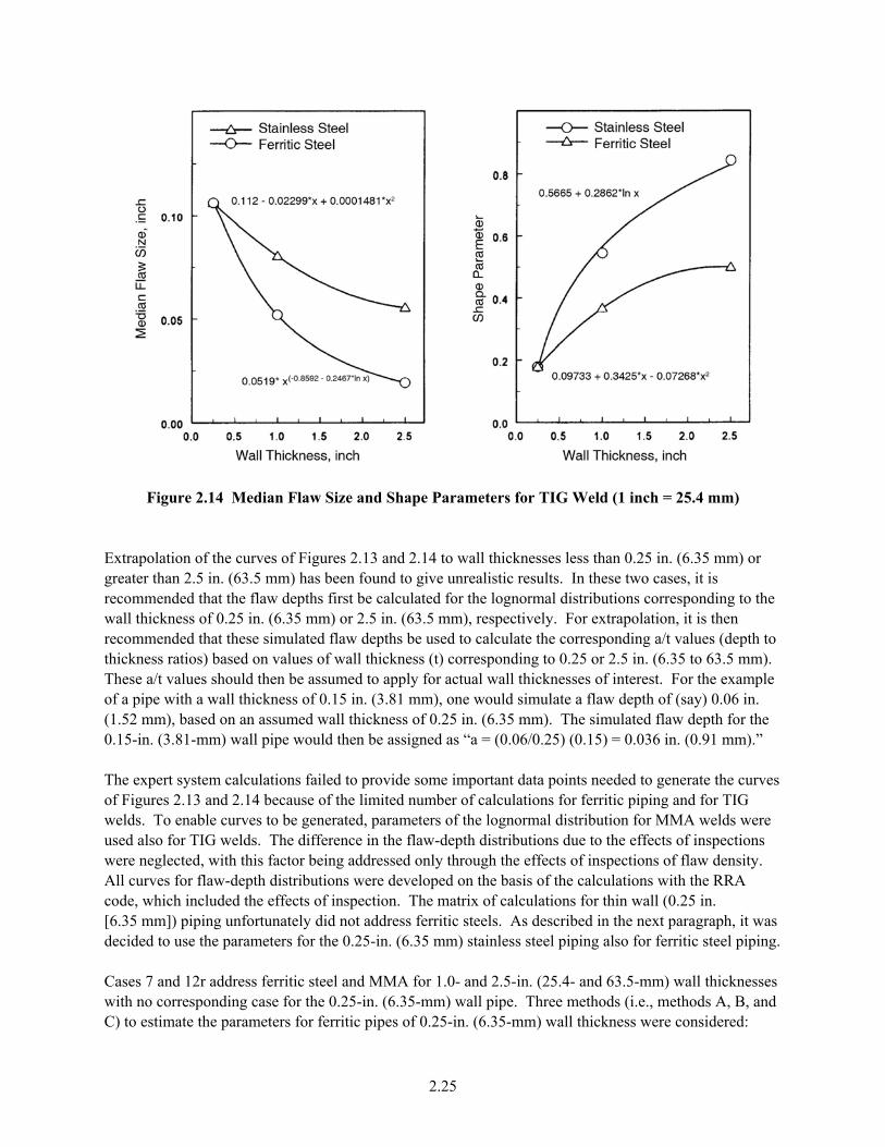
Figure 2.14 Median Flaw Size and Shape Parameters for TIG Weld (1 inch = 25.4 mm) Extrapolation of the curves of Figures 2.13 and 2.14 to wall th nes 0. (6.3 r greater than 2.5 in. (63.5 been d to ealis resu tw es, irecommended that the flaw depths first be calculated for the l orm ons spo the wall thickness of 0.25 in. (6.35 mm) o . (6 , respectively. For extrapolation, it irec d t thes flaw hs b cal te t din values (depth to thickness ratios) based on values of wall thickness (t) corresponding to 0.25 or 2.5 in. (6.35 to 63.5 mm).
hese a/t values should then be assumed to apply for actual wall thicknesses of interest. For the example f a pipe with a wall thickness of 0.15 in. (3.81 mm), one would simulate a flaw depth of (say) 0.06 in.
mm). The simulated flaw depth for the 0.15-in. (3.81-mm) wall pipe would then be assigned as “a = (0.06/0.25) (0.15) = 0.036 in. (0.91 mm).”
ves
were
ections of flaw density. ll curves for flaw-depth distributions were developed on the basis of the calculations with the RRA
as iping.
e for the 0.25-in. (6.35-mm) wall pipe. Three methods (i.e., methods A, B, and
) to estimate the parameters for ferritic pipes of 0.25-in. (6.35-mm) wall thickness were considered:
ick ses less than 25 in. 5 mm) o mm) has foun give unr tic lts. In these o cas t is
ogn al distributi corre nding to r 2.5 in 3.5 mm) s then
ommende hat e simulated dept e used to cula he correspon g a/t
To(1.52 mm), based on an assumed wall thickness of 0.25 in. (6.35
The expert system calculations failed to provide some important data points needed to generate the curof Figures 2.13 and 2.14 because of the limited number of calculations for ferritic piping and for TIG welds. To enable curves to be generated, parameters of the lognormal distribution for MMA weldsused also for TIG welds. The difference in the flaw-depth distributions due to the effects of inspections were neglected, with this factor being addressed only through the effects of inspAcode, which included the effects of inspection. The matrix of calculations for thin wall (0.25 in. [6.35 mm]) piping unfortunately did not address ferritic steels. As described in the next paragraph, it wdecided to use the parameters for the 0.25-in. (6.35 mm) stainless steel piping also for ferritic steel p Cases 7 and 12r address ferritic steel and MMA for 1.0- and 2.5-in. (25.4- and 63.5-mm) wall thicknesseswith no corresponding casC
2.25
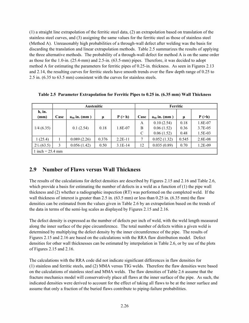
(1) a straight line extrapolation of the ferritic steel data, (2) an extrapolation based on translation stainless steel curves, and (3) assigning the same values for the ferritic steel as those of stainless steel (Method A). Unreasonably high probabilities of a through-wall defect after welding was the basis for discarding the translation and linear extrapolation methods. Table 2.5 summarizes the results of applying the three alternative methods. The probability of a through-wall defect for method A is on the same order as those for the 1.0-in. (25.4-mm) and 2.5-in. (63.5-mm) pipes. Therefore, it was decided
of the
to adopt method A for estimating the parameters for ferritic pipes of 0.25-in. thickness. As seen in Figures 2.13 and 2.14, the resulting curves for ferritic steels have smooth trends over the flaw depth range of 0.25 to 2.5 in. (6.35 to 63.5 mm) consistent with the curves for stainless steels.
Table 2.5 Parameter Extrapolation for Ferritic Pipes to 0.25 in. (6.35 mm) Wall Thickness
Austenitic Ferritic h, in. (mm) Case a50 in. (mm ) µ P (> h) Case a50 in. (mm ) µ P (>h)
1/4 (6.35) 0.1 (2.54) 0.18 1.8E-07 A B C
0.10 (2.54) 0.06 (1.52) 0.06 (1.52)
0.18 0.36 0.48
1.8E-07 3.7E-05 1.5E-03
1 (25.4) 1 0.089 (2.26) 0.376 2.2E-11 7 0.052 (1.32) 0.545 2.8E-08 2½ (63.5) 3 0.056 (1.42) 0.50 3.1E-14 12 0.035 (0.89) 0.70 1.2E-09 1 inch = 25.4 mm
.9 Number of Flaws versus Wall Thickness
he results of the calculations for defect densities are described by Figures 2.15 and 2.16 and Table 2.6, hich provide a basis for estimating the number of defects in a weld as a function of (1) the pipe wall
thickness and (2) whether a radiographic inspection (R med on the completed weld. If the all thickness of interest is greater than 2.5 in. (63.5 mm) or less than 0.25 in. (6.35 mm) the flaw
dens e data in terms of the semi-log scales as displayed by Figures 2.15 and 2.16.
The defect density is expressed as the number of defects per inch of weld, with the weld length measured along the inner surface of the pipe circumference. The total number of defects within a given weld is determined by multiplying the defect density by the inner circumference of the pipe. The results of Figures 2.15 and 2.16 are based on the calculations with the RRA flaw distribution model. Defect densities for other wall thicknesses can be estimated by interpolation in Table 2.6, or by use of the plots of Figures 2.15 and 2.16. The calculations with the RRA code did not indicate significant differences in flaw densities for (1) stainless and ferritic steels, and (2) MMA versus TIG welds. Therefore the flaw densities were based on the calculations of stainless steel and MMA welds. The flaw densities of Table 2.6 assume that the fracture mechanics model will conservatively place all flaws at the inner surface of the pipe. As such, the indicated densities were derived to account for the effect of taking all flaws to be at the inner surface and assume that only a fraction of the buried flaws contribute to piping-failure probabilities.
2
Tw
T) was perforw
ities can be estimated from the values given in Table 2.6 by an extrapolation based on the trends ofth
2.26
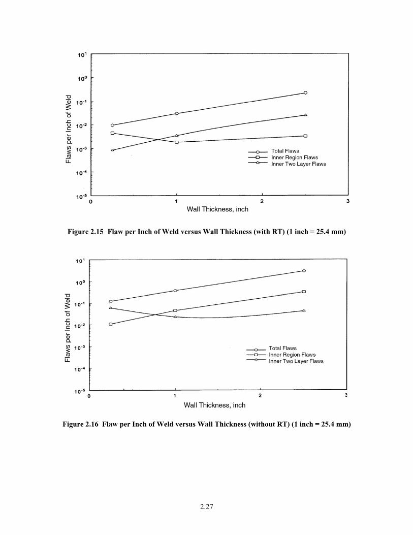
Figure 2.15 Flaw per Inch of Weld versus Wall Thickness (with RT) (1 inch = 25.4 mm)
Figure 2.16 Flaw per Inch of Weld versus Wall Thickness (without RT) (1 inch = 25.4 mm)
2.27
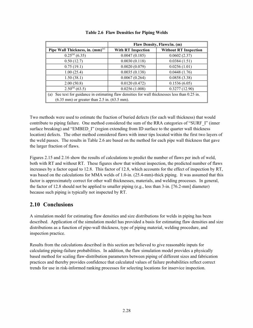
Table 2.6 Flaw Densities for Piping Welds
Flaw Density, Flaws/in. (m) Pipe Wall Thickness, in. (mm)(a) With RT Inspection Without RT Inspection
0.25(a) (6.35) 0.0047 (0.185) 0.0602 (2.37) 0.50 (12.7) 0.0030 (0.118) 0.0384 (1.51) 0.75 (19.1) 0.0020 (0.079) 0.0256 (1.01) 1.00 (25.4) 0.0035 (0.138) 0.0448 (1.76) 1.50 (38.1) 0.0067 (0.264) 0.0858 (3.38) 2.00 (50.8) 0.0120 (0.472) 0.1536 (6.05) 2.50(a) (63.5) 0.0256 (1.008) 0.3277 (12.90)
(a) See text for guidance in estimating flaw densities for wall thicknesses less than 0.25 in. (6.35 mm) or greater than 2.5 in. (63.5 mm).
Two methods were used to estimate the fraction of buried defects (for each wall thickness) that would contribute to piping failure. One method considered the sum of the RRA categories of “SURF_I” (inner surface breaking) and “EMBED_I” (region extending from ID surface to the quarter wall thickness location) defects. The other method considered flaws with inner tips located within the first two layers of the weld passes. The results in Table 2.6 are based on the method for each pipe wall thickness that gave he larger fraction of flaws. t
Figures 2.15 and 2.16 show the results of calculations to predict the number of flaws per inch of weld, both with RT and without RT. These figures show that without inspection, the predicted number of flawincreases by a factor equal to 12.8. This factor of 12.8, which accounts for the effect of inspection by RT, was based on the calculations for MMA welds of 1.0-in. (25.4-mm)-thick piping. It was assumed that thisfactor is approximately correct for other wall thicknesses, materials, and welding processes. In general, the factor of 12.8 should not be applied to smaller piping (e.g., less than 3-in. [76.2-mm] diameter) because such piping is typically not inspected by RT.
s
s as a function of pipe-wall thickness, type of piping material, welding procedure, and
2.10 Conclusions
A simulation model for estimating flaw densities and size distributions for welds in piping has been described. Application of the simulation model has provided a basis for estimating flaw densities and size
istributiondinspection practice. Results from the calculations described in this section are believed to give reasonable inputs for calculating piping-failure probabilities. In addition, the flaw simulation model provides a physically based method for scaling flaw-distribution parameters between piping of different sizes and fabrication practices and thereby provides confidence that calculated values of failure probabilities reflect correct trends for use in risk-informed ranking processes for selecting locations for inservice inspection.
2.28
3 Parametric Calculations for Fatigue
3.1 Introduction
Piping systems experience cyclic stresses caused by anticipated plant transients (e.g., rapid cooling of the piping during auxiliary feedwater initiation following a scram) and unanticipated transients (e.g., checvalve leakage). This section describes the probabilistic fracture mechanics (PFM) computer code and the structural mechanics modeling approach that PNNL has used to simulate the effects of these cyclic fatigue stresses on the reliability of reactor piping. Also described are sensitivity calculations that evaluate the effects of modeling assumptions. The overall objective of the study was to develop a pipreliability model that could be used to simulate the effects of alternative inservice insp
k-
ing ection strategies so
at inspection methods (flaw-detection capability) and inspection intervals can be established in a
s for
nal
al h
rack-tip stress intensity factors (Harris t al. 1992).
bility. the results are presented as sets of curves
nd tables.
ped the PFM computer ode pc-PRAISE (Harris et al. 1992) for the NRC to support probabilistic analyses of piping containing ircumferential surface-breaking cracks. This code has been used extensively for the calculations
described in the present report.
thmanner consistent with goals for the reliability of the piping systems. The calculations of this section (and Sections 4 and 5) were performed in a structured parametric format, with the parameters selected to cover the range of pipe sizes, piping materials, and operating stresses relevant to reactor piping systems. This permitted estimates of piping reliability (including the effects of alternative inspection strategies) to be made without incurring the high costs of individual calculationthe hundreds of welds and fittings that make up the piping systems of interest. Probabilistic fracture mechanics calculations often assume that the stress state in the pipe wall is uniform through the thickness of the pipe wall. This approach is appropriate for the stresses caused by interpressure. It is a good approximation for the bending of piping caused by thermal expansion of pipe systems, but it does not address through-wall stress gradients caused by radial thermal gradients, residustresses, or geometric discontinuities. This section includes calculations that evaluate the effects of sucthrough-wall stress variations by applying the capability of pc-PRAISE to simulate radial gradient stresses with the so-called “g-function” approach for calculating ce The first part of this section describes the pc-PRAISE code, compares the results of the pc-PRAISE and PARIS codes, and describes details of the fracture mechanics model used for predicting piping reliaParametric calculations are then performed using the model, anda 3.2 Piping Reliability Code pc-PRAISE
The use of PFM models to simulate the growth of the cracks in welds that pass undetected during piping fabrication has become a common practice in recent years. Probabilistic fracture mechanics evaluations combine the methods of reliability theory and fracture mechanics to assess the structural reliability of components containing defects. Lawrence Livermore National Laboratory develocc
3.1
The pc-PRAISE code calculates failure probabilities caused by the growth of pre-existing cracks caused by cyclic loads, and by the initiation and growth of stress-corrosion cracks. The model simulates the growth of two-dimensional cracks in both their length and depth directions with the initial crack sizes described by statistical distributions. The crack distributions are modified as a result of preservice and inservice inspections, with the probability of flaw detection (POD) expressed as a function of crack size. Limit states for piping loads and crack sizes are used to calculate the probabilities of leak and break. The criterion for pipe break is that of the net section stress becoming equal to the material flow stress. A small leak occurs if the stable crack growth results in a through-wall crack. A big leak occurs if the crack opening area (related to the through-wall crack length and applied loads) is such that the leakage exceeds the prescribed flow rate corresponding to the operating definition of a large leak. Because of typically low probabilities of failure and the large number of input parameters, a Monte Carlo simulation with variance reduction by stratified sampling is applied to calculate failure probabilities. The schematic diagram of the steps in the pipe reliability calculations with pc-PRAISE are presented in Figure 3.1. Starting at the upper left-hand corner of the diagram, a new weld in a pipe is assumed to begin its life with a distribution of welding flaws. This distribution is immediately modified as a result of post-weld inspections and repairs. Once the plant is placed into operation, there are cyclic stresses that cause the remaining cracks to grow. Some cracks can be sufficiently large and/or will grow at sufficiently high rates such that their depths could penetrate the pipe wall. In some cases, there will be inservice inspections that detect some of the growing cracks in a timely manner. In these cases, the damaged pipe will be repaired. In other cases, the growing crack will penetrate the wall of the pipe and thereby cause a leak. In many cases, this leakage will be small and the leakage will be detected. In these cases, the pipe will be repaired before a big leak or pipe break (loss of coolant accident [LOCA]) occurs. The pc-PRAISE model predicts the rate of leakage for through-wall cracks in pipes and calculates the probability that the leakage rates are sufficiently large to cause the LOCA type of event. In summary, the Monte Carlo simulation as performed by pc-PRAISE involves a large number of trials. The outcome of each trial is (1) there is no through-wall crack and the pipe does not fail, (2) a small leak occurs, (3) a large leak occurs, or 4) the pipe fails in the mode of a break or LOCA. One objective of PNNL’s studies was to compare the numerical results and procedures used in the pc-
RAISE code with other similar computer codes. One of these efforts consisted of a set of benchmarking
s
urckner-Foit et al. (1989) compared results from the PARIS code and the pc-PRAISE code in a second
Pcalculations that compared predictions of pc-PRAISE with predictions made by a similar code that Westinghou e Electric Corporation developed (Bishop 1997). Bbenchmarking effort. The PARIS code was developed at the Nuclear Research Center Karlsruhe(Germany) for predicting the reliability of components containing through-wall or surface cracks. Both the pc-PRAISE and PARIS codes use the Monte Carlo simulation techniques to determine failure probabilities, but use different variance-reduction techniques to reduce the computational effort needed toperform the Monte Carlo simulation. The PARIS code uses importance sampling (as used also by Bishop1997) whereas the pc-PRAISE code uses stratified sampling (Harris et al. 1992).
3.2
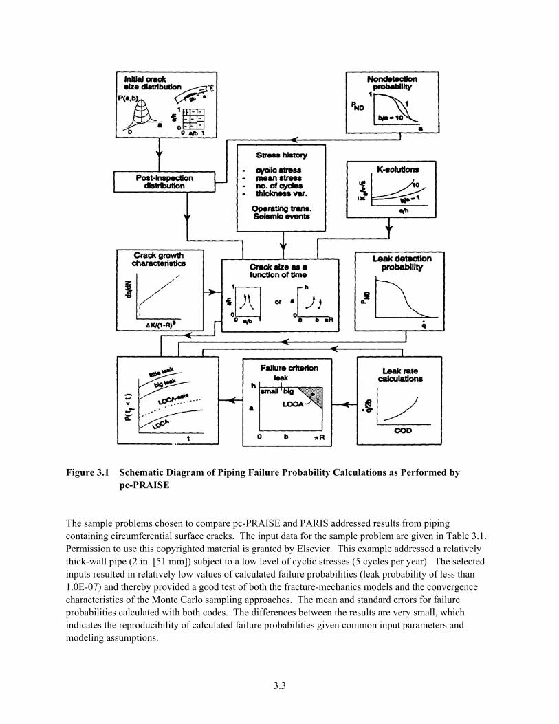
Figure 3.1 Schematic Diagram of Piping Failure Probability Calculations as Performed by
pc-PRAISE
ampling approaches. The mean and standard errors for failure robabilities calculated with both codes. The differences between the results are very small, which
indicates the reproducibility of calculated failure probabilities given common input parameters and modeling assumptions.
The sample problems chosen to compare pc-PRAISE and PARIS addressed results from piping containing circumferential surface cracks. The input data for the sample problem are given in Table 3.1. Permission to use this copyrighted material is granted by Elsevier. This example addressed a relatively thick-wall pipe (2 in. [51 mm]) subject to a low level of cyclic stresses (5 cycles per year). The selectedinputs resulted in relatively low values of calculated failure probabilities (leak probability of less than 1.0E-07) and thereby provided a good test of both the fracture-mechanics models and the convergence characteristics of the Monte Carlo sp
3.3
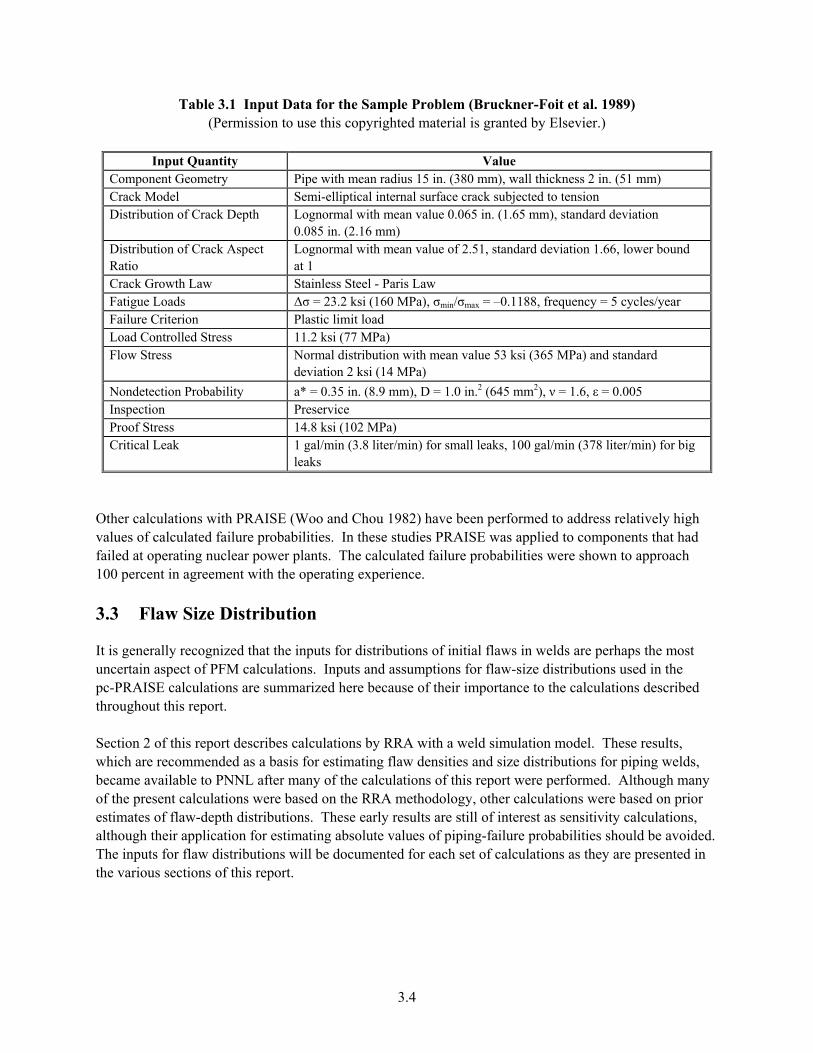
Table 3.1 Input Data for the Sample Problem (Bruckner-Foit et al. 1989) (Permission to use this copyrighted material is granted by Elsevier.)
Input Quantity Value
Component Geometry Pipe with mean radius 15 in. (380 mm), wall thickness 2 in. (51 mm) Crack Model Semi-elliptical internal surface crack subjected to tension D
0.085 in. (2.16 mm) istribution of Crack Depth Lognormal with mean value 0.065 in. (1.65 mm), standard deviation
Distribution of Crack Aspect Lognormal with mean value of 2.51, standard deviation 1.66, lower bound Ratio at 1 Crack Growth Law Stainless Steel - Paris Law Fatigue Loads ∆σ = 23.2 ksi (160 MPa), σmin/σmax = –0.1188, frequency = 5 cycles/year Failure Criterion Plastic limit load Load Controlled Stress 11.2 ksi (77 MPa) Flow Stress Normal distribution with mean value 53 ksi (365 MPa) and standard
deviation 2 ksi (14 MPa) Nondetection Probability a* = 0.35 in. (8.9 mm), D = 1.0 in.2 (645 mm2), ν = 1.6, ε = 0.005 In Preservice spection Proof Stress 14.8 ksi (102 MPa) Critical Leak 1 gal/min (3.8 liter/min) for small leaks, 100 gal/min (378 liter/min) for big
leaks Other calculations with PRAISE (Woo and Chou 1982) have been performed to address relatively high
nts that had failed at operating nuclear power plants. The calculated failure probabilities were shown to approach
ds,
re probabilities should be avoided. he inputs for flaw distributions will be documented for each set of calculations as they are presented in
values of calculated failure probabilities. In these studies PRAISE was applied to compone
100 percent in agreement with the operating experience. 3.3 Flaw Size Distribution
It is generally recognized that the inputs for distributions of initial flaws in welds are perhaps the most uncertain aspect of PFM calculations. Inputs and assumptions for flaw-size distributions used in the pc-PRAISE calculations are summarized here because of their importance to the calculations described throughout this report. Section 2 of this report describes calculations by RRA with a weld simulation model. These results, which are recommended as a basis for estimating flaw densities and size distributions for piping welbecame available to PNNL after many of the calculations of this report were performed. Although many of the present calculations were based on the RRA methodology, other calculations were based on prior estimates of flaw-depth distributions. These early results are still of interest as sensitivity calculations, although their application for estimating absolute values of piping-failuTthe various sections of this report.
3.4
3.5
detected
m odel does not address. These flaws can represent very small fabrication defects below the usual threshold flaw sizes of concern, or
ner
ld b des tables or numerical histograms of the sizes and locations of the defects within a weld. For the purposes of the calculations with pc-PRAISE,
se stresses are nique and plant specific for each location within the piping systems of a given plant. An evaluation of
ematical form of the crack growth rate equations.
Two broad categories of flaws are addressed as follows: • Larger flaws whose depths approach or exceed the thickness of the weld beads (or layers) that make
up the weld. These are fabrication flaws associated with the welding process that could be by preservice inspection and that may be repaired if detected. As noted above, the numbers and sizesof these larger flaws were estimated either using the RRA expert system model as described in Section 2, or, in the case of other calculations, were based on earlier estimates of flaw-distribution parameters.
• S all flaws below the detection and repair thresholds that the RRA m
they can represent flaws that initiate by fatigue under service conditions. Only a few calculations of this report address this category of small flaws because the category of larger fabrication flaws is usually the primary contributor to calculated piping-failure probabilities. All calculations for the small-flaw category were based on a uniform distribution of flaw depths ranging from 0.002 to 0.010 in. (0.05 to 0.25 mm), with the assumption that each pipe weld had one such flaw at the insurface of the pipe.
It shou e noted that the RRA weld simulation model provi
these histograms were approximated by standard lognormal distributions using the approach described in Section 2 of this report. 3.4 Parametric Treatment of Cyclic Stresses Using the Q-Factor
Piping stresses along with the operational transients that govern the cyclic nature of theupiping reliability in complete detail might involve thousands of calculations to address all locations of interest for even a single plant. Therefore, the evaluations of this report were performed using a parametric approach to minimize the number of calculations needed to establish trends for piping-failure probabilities and to establish the effects of inservice inspections on these failure probabilities. With the parametric approach, it was possible to cover the full range of stresses and cyclic conditions of interest with a limited number of calculations. For fatigue of stainless steel piping, it was possible to further reduce the number of calculations by using a single numerical parameter (Q-factor) that captured the combined effect of cyclic stress level and number of stress cycles. The Q-factor approach was made possible by the simple Paris Law crack growth equation (da/dN = (C∆σ4)) that applies to stainless steel. Attempts to identify a similar factor for fatigue of ferritic steels (also for stress-corrosion cracking of stainless steels) were unsuccessful because of the more complex math For fatigue of stainless steels, the parameter Q was defined as ( )4Q Nα σ= ∆ (3.1)
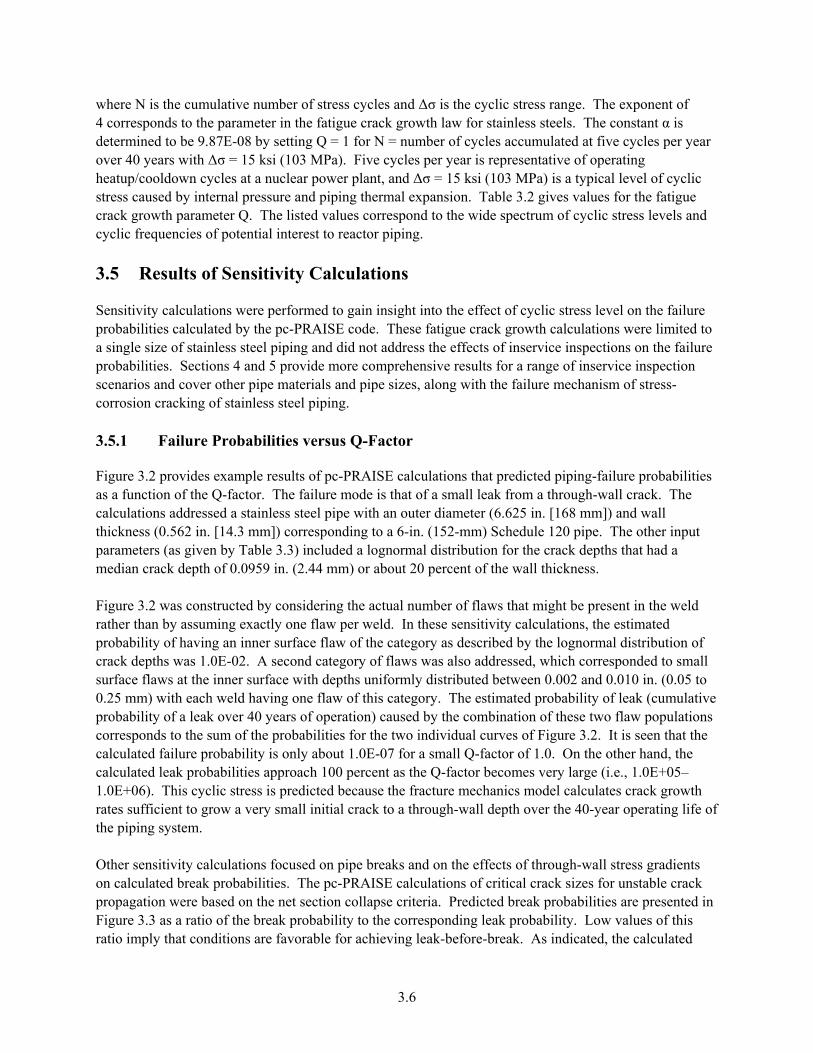
where N is the cumulative number of stress cycles and ∆σ is the cyclic stress range. The exponent of 4 corresponds to the parameter in the fatigue crack growth law for stainless steels. The constant α is determined to cles accumulated at five cycles per year over 40 ye e of operating heatup/cooldown i (103 MPa) is a typical level of cyclic stress caused by internal pressure and piping thermal expansion. Table 3.2 gives values for the fatigue
k grow ide spectrum of cyclic stress levels and ic freq
Results of Sensitivity Calculations
sitivity calcu fect of cyclic stress level on the failure abilities calculated by ack growth calculations were limited to gle siz ts of inservice inspections on the failure ab lts for a range of inservice inspection ar nd cover other pipe materials and pipe sizes, along with the failure mechanism of stress-os rac
1 Failu
re at predicted piping-failure probabilities fu leak from a through-wall crack. The ula s addressed a stai 6.625 in. [168 mm]) and wall kn 0.562 other input meters ion for the crack depths that had a ian crack f the wall thickness.
re 3.2 laws that might be present in the weld er than itivity calculations, the estimated ability of having an inner surface fl the lognormal distribution of k depths was ddressed, which corresponded to small ace fla d between 0.002 and 0.010 in. (0.05 to mm) wit stimated probability of leak (cumulative ability of a leak over 40 years of operation) caused by the combination of these two flaw populations esponds t e 3.2. It is seen that the ulated factor of 1.0. On the other hand, the ulated leak pr i mes very large (i.e., 1.0E+05–+06). This cyclic stress is predicted because the fracture chanics model calculates crack growth
s sufficient to grow a very small initial crack t h l depth over the 40-year operating life of piping sy
Other senon calculated break probabilities. The pc-PRAISE cal f critical crack sizes for unstable crack propagation were cted break probabilities are presented in Figure 3.3 as a ra leak probability. Low values of this ratio imply that conditions are favorable for achieving leak-before-break. As indicated, the calculated
be wit
9.87h ∆ cycles at a nuclear power plant, and
E-0σ =
8 b15 k
y sesi (
ttin103
g Q MP
= 1a).
for Fiv
N =e c
nuycle
mbes pe∆σ
r or year is representativ= 15
f cy
ksars
craccycl 3.5
Senproba sinprobscencorr 3.5.
Figuas acalcthicparamed Figurathprobcracsurf0.25probcorrcalccalc1.0Eratethe
th uen
paracie
mes of
ter pot
Q. enti
Theal in
listtere
ed vst t
aluo re
es cacto
orrer pi
spopin
nd tg.
o the w
lations were performed to gain insight into the ef the pc-PRAI
stee and
SE code. These fad di mo
tigue cre eve r
e os.
f st Sec
ainltion
ess s 4
l pip 5 p
ingrov
anide
d nore co
t admp
drereh
ss thensi
ffecesuilitie
ios aion c
3.2 nctiotion
ess (
king of
re P
sta
rob
inle
ab
ss s
iliti
teel
es v
pip
er
ing.
sus
Q-Factor
prn
ovidof th
es ee Q
xam-fa
ple results of pc-PRAISE calctor
cula of a
tion sm
m
s thall eter (
. Thnless steel pi
e failure mpe with an
ode is that outer dia
in. [ven th o
14.3by Table 3.3) if 0.
m
095
m])
9 in
corr
. (2
espnclu.44
ondded
mm
ing a l
) or
to aogn abo
6-in. (152-mm) Schedule 120 pipe. The ormut 2
(as gi dep
al d0 p
istrerce
ibutnt o
wa by
s co ass
nstrum
ucting
ed bexa
y coctly
nsione
der fla
ing w paw of the cat
the er w
actueld
al n. In
egor
umb the
y
er se s as described by
of fens
1.0e i
ch w
E-0nner
eld
2. A su ha
serfacving
cone wi on
d cath de fl
tegept
aw
ory hs uof th
of fnifois c
lawrmlategory
s way di
s alstri. T
so abutehe e
ws at thh ea
o thlure
e su prooba
m obabbil
f thilityties
e pr is
app
obaonlyroa
bili ab
ch 1
ties out 00
for 1.0Eperc
the -07ent
two foras the Q-factor beco
ind a s
ividual curves of Figurmalfai l Q-
mewal
s orediing
o a t
ks and on the effects of through-wall stress gradients
cri cor
ro
culateriaresp
ugh-
tion. Pond
stem
vity
.
calc
bastio o
siti ulat
ed f th
ion
on te b
s fo
he nreak
cuse
et s pro
d o
ectibab
n pi
on cilit
pe b
ollay to
rea
pse the
3.6
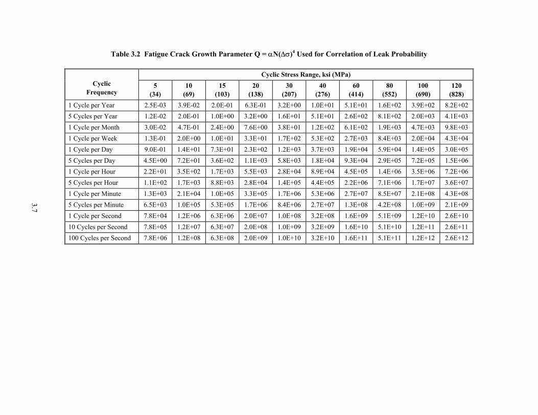
Table 3.2 Fatigue Crack Growth Parame )4 or Correlation of Leak Probability
clic Stre ange, ksi (MPa)
ter Q = αN(∆σ Us
ss R
ed f
CyCyclic
Frequency (32
(130
(40
(276) 60
(414) 80
(552) 100
(690) 120
(828) 5 4)
10 (69)
15 03) (1
0 38) 207)
1 Cycle per Year 5 3. 1 .3 3. 1.0E+01 5.1E+01 1.6E+02 3.9E+02 8.2E+02 2. E-03 9E-02 2.0E-0 6 E-01 2E+00 5 Cycles per Year 2 2. 01 00 2E 1. 5.1E+01 2.6E+02 8.1E+02 2.0E+03 4.1E+03 1. E-02 0E- 1.0E+ 3. +00 6E+01 1 Cycle per Month 3.0E-02 4. 01 +00 6E 3. 1.2E+02 6.1E+02 1.9E+03 4.7E+03 9.8E+03 7E- 2.4E 7. +00 8E+01 1 Cycle per Week 1.3E-01 2.0E+00 +01 3.3E 1. 5.3E+02 2.7E+03 8.4E+03 2.0E+04 4.3E+04 1.0E +01 7E+02 1 Cycle per Day 9.0E-01 1.4E+01 01 2.3E 1. 3.7E+03 1.9E+04 5.9E+04 1.4E+05 3.0E+05 7.3E+ +02 2E+03 5 Cycles per Day 4.5E+00 7.2E+01 3.6E+02 1.1E 5. 1.8E+04 9.3E+04 2.9E+05 7.2E+05 1.5E+06 +03 8E+03 1 Cycle per Hour .5E 2. 8.9E+04 4.5E+05 1.4E+06 3.5E+06 7.2E+06 2.2E+01 3.5E+02 1.7E+03 5 +03 8E+04 5 Cycles per Hour 8E 1. 4.4E+05 2.2E+06 7.1E+06 1.7E+07 3.6E+07 1.1E+02 1.7E+03 8.8E+03 2. +04 4E+05 1 Cycle per Minut E 3E 1. 5.3E+06 2.7E+07 8.5E+07 2.1E+08 4.3E+08 e 1.3E+03 2.1 +04 1.0E+05 3. +05 7E+06 5 Cycles per Minut E 7E 8.4E+ 2.7E+07 1.3E+08 4.2E+08 1.0E+09 2.1E+09 e 6.5E+03 1.0 +05 5.3E+05 1. +06 06 1 Cycl r Secon E 0E 1.0E+ 3.2E+08 1.6E+09 5.1E+09 1.2E+10 2.6E+10 e pe d 7.8E+04 1.2 +06 6.3E+06 2. +07 08 10 Cycles per Seco E .3 0E 1.0E+ 3.2E+09 1.6E+10 5.1E+10 1.2E+11 2.6E+11 nd 7.8E+05 1.2 +07 6 E+07 2. +08 09 100 C ycles per Se 7.8E+06 E .3 8 0E 1.0E+ 3.2E+10 1.6E+11 5.1E+11 1.2E+12 2.6E+12 10 +09cond 1.2 +08 6 E+0 2.
3.7
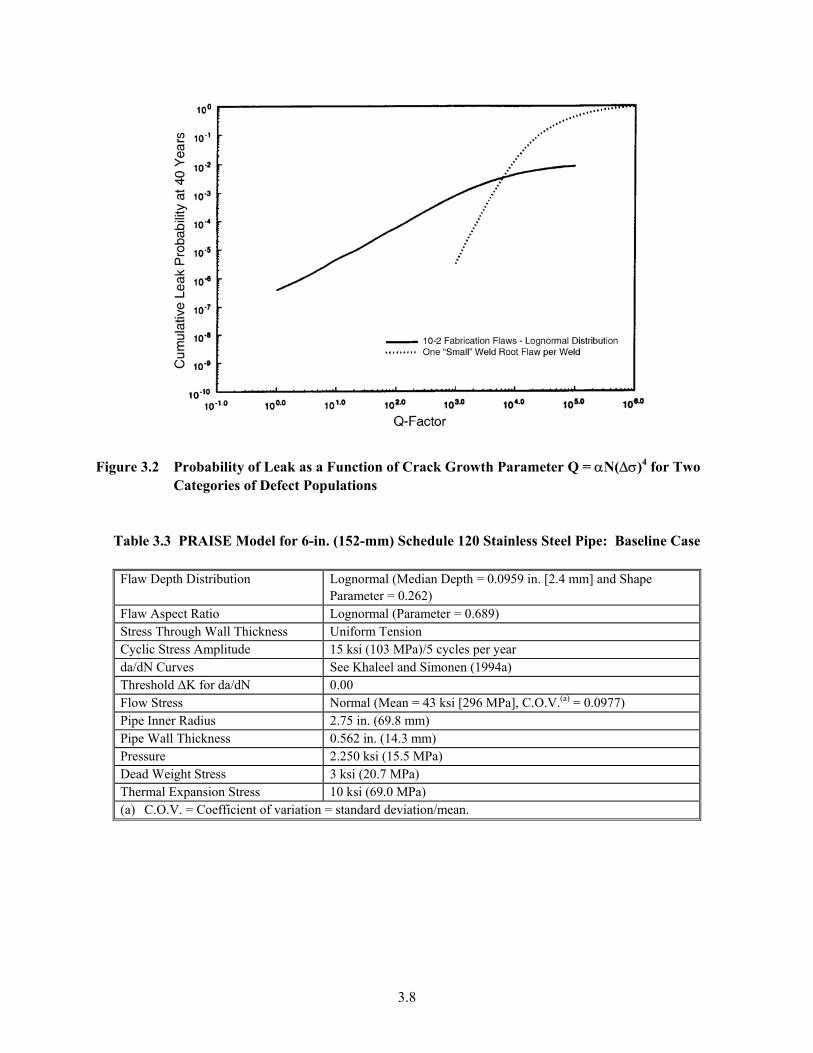
Figure 3.2 Probability of Leak as a Function of Crack Growth Parameter Q = αN(∆σ)4 for Two
Categories of Defect Populations
Table 3.3 PRAISE Model for 6-in. (152-mm) Schedule 120 Stainless Steel Pipe: Baseline Case
Flaw Depth Distribution Lognormal (Median Depth = 0.0959 in. [2.4 mm] and Shape Parameter = 0.262)
Flaw Aspect Ratio Lognormal (Parameter = 0.689) Stress Through Wall Thickness Uniform Tension Cyclic Stress Amplitude 15 ksi (103 MPa)/5 cycles per year da/dN Curves See Khaleel and Simonen (1994a) Threshold ∆K for da/dN 0.00 Flow Stress Normal (Mean = 43 ksi [296 MPa], C.O.V.(a) = 0.0977) Pipe Inner Radius 2.75 in. (69.8 mm) Pipe Wall Thickness 0.562 in. (14.3 mm) Pressure 2.250 ksi (15.5 MPa) Dead Weight Stress 3 ksi (20.7 MPa) Thermal Expansion Stress 10 ksi (69.0 MPa) (a) C.O.V. = Coefficient of variation = standard deviation/mean.
3.8
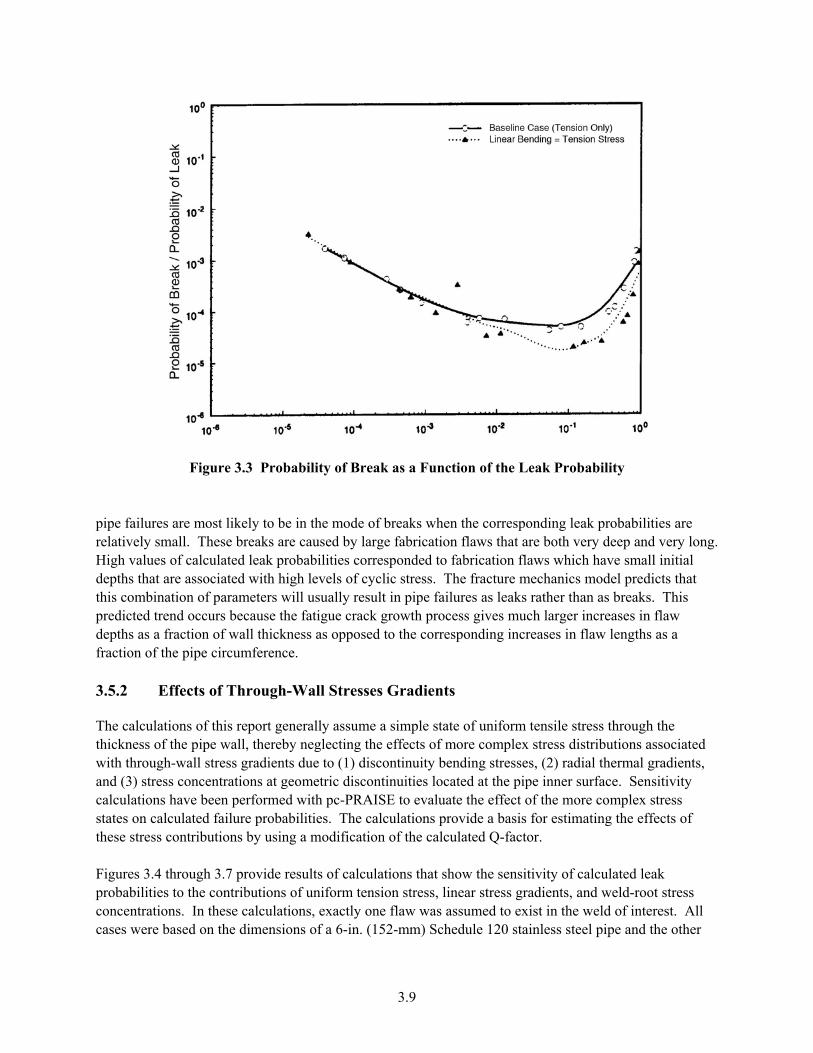
Figure 3.3 Probability of Break as a Function of the Leak Probability pipe failures are most likely to be in the mode of breaks when the corresponding leak probabilities are relatively small. These breaks are caused by large fabrication flaws that are both very deep a d very long.
igh values of calculated leak probabilities corresponded to fabrication flaws which have sm ll initial
redicted trenepths as a fraction of wall thickness as opposed to the corresponding increases in flaw lengths as a
e pipe circumference.
The calculatiickness of wall, thereby neglecting the effects of more complex stress distributions associated
l r
naH
depths that are associated with high levels of cyclic stress. The fracture mechanics model predicts that this combination of parameters will usually result in pipe failures as leaks rather than as breaks. This
d occurs because the fatigue crack growth process gives much larger increases in flaw pdfraction of th 3.5.2 Effects of Through-Wall Stresses Gradients
ons of this report generally assume a simple state of uniform tensile stress through the the pipe th
with through-wall stress gradients due to (1) discontinuity bending stresses, (2) radial thermal gradients, and (3) stress concentrations at geometric discontinuities located at the pipe inner surface. Sensitivity calculations have been performed with pc-PRAISE to evaluate the effect of the more complex stress states on calculated failure probabilities. The calculations provide a basis for estimating the effects of these stress contributions by using a modification of the calculated Q-factor. Figures 3.4 through 3.7 provide results of calculations that show the sensitivity of calculated leak probabilities to the contributions of uniform tension stress, linear stress gradients, and weld-root stress concentrations. In these calculations, exactly one flaw was assumed to exist in the weld of interest. Alcases were based on the dimensions of a 6-in. (152-mm) Schedule 120 stainless steel pipe and the othe
3.9
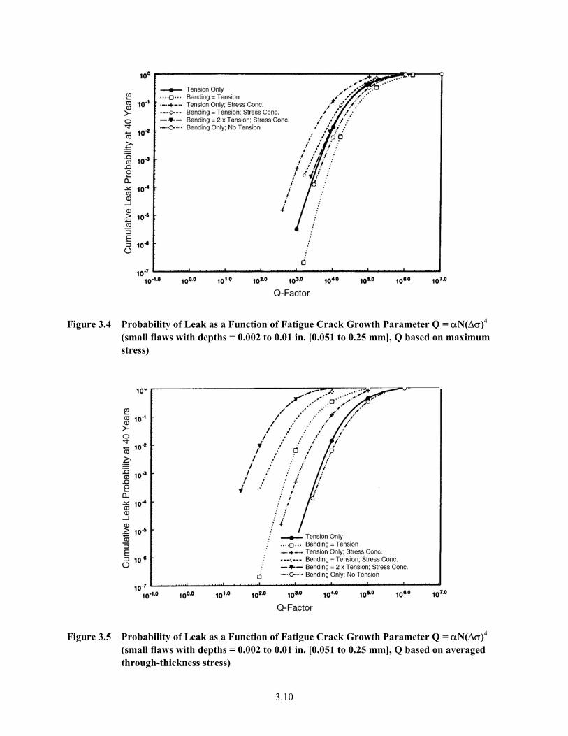
Figure 3.4 Probability of Leak as a Function of Fatigue Crack Growth Parameter Q = αN(∆σ)
(small flaws with depths = 0.002 to 0.01 in. [0.051 to 0.25 mm], Q based on maximum stress)
4
Figure 3.5 Probability of Leak as a Function of Fatigue Crack Growth Parameter Q = αN(∆σ)4
(small flaws with depths = 0.002 to 0.01 in. [0.051 to 0.25 mm], Q based on averaged through-thickness stress)
3.10
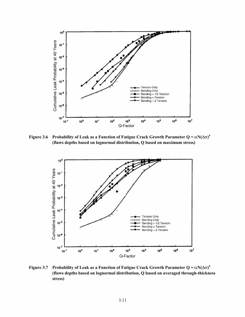
3.11
Figure 3.7 lity of Leak as a Fatigue Crack Growth Parameter Q = αN(∆σ)4
ep s based on lognormal distribution, Q based on averaged through-thickness )
Figure 3.6 Probability Fatigue Crack Growth Parameter Q = αN(∆σ)4
(flaws depths based on lognormal distribution, Q based on maximum stress)
Probabi(flaws dstress
Function of th
of Leak as a Function of
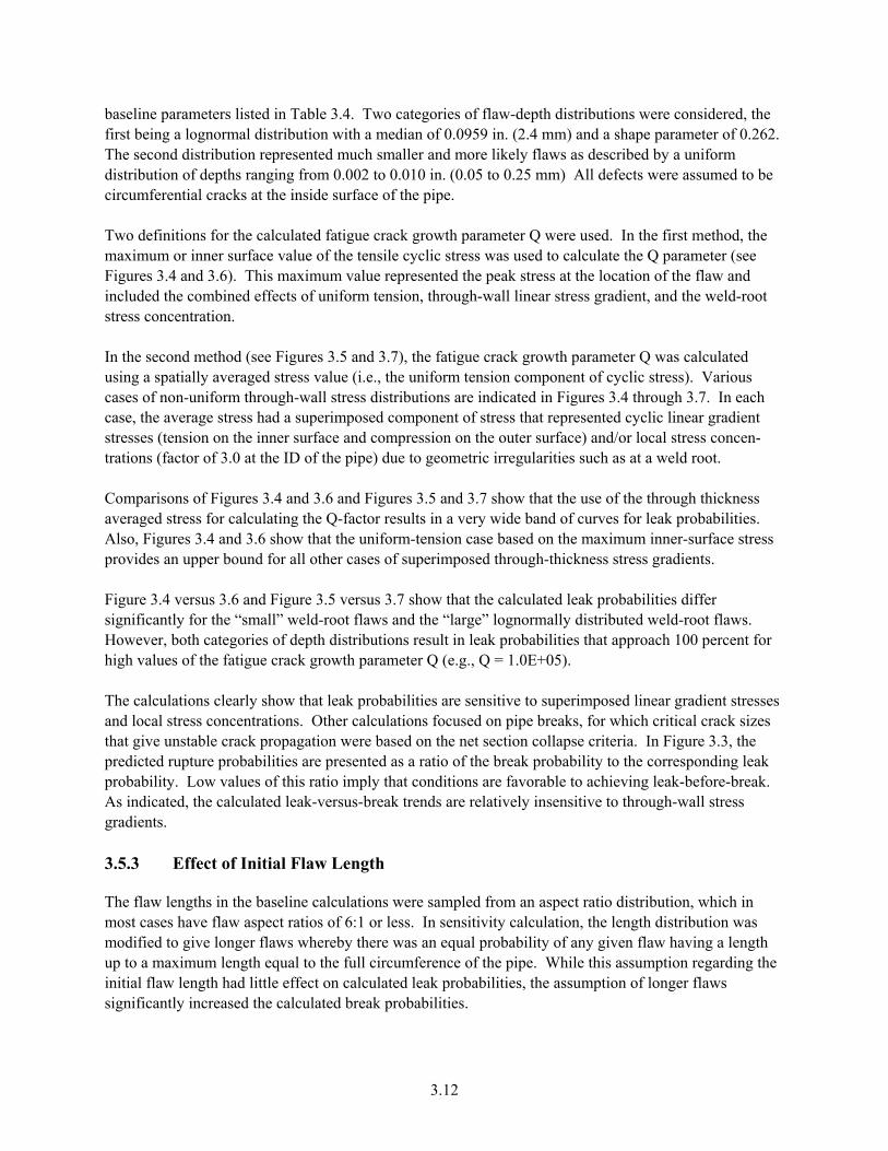
baseline parameters listed in Table 3.4. Two categories of flaw-depth distributions were considered, the first being a lognormal distribution with a median of 0.0959 in. (2.4 mm) and a shape parameter of 0.262.
e
stress at the location of the flaw and cluded the combined effects of uniform tension, through-wall linear stress gradient, and the weld-root
gue crack growth parameter Q was calculated sing a spatially averaged stress value (i.e., the uniform tension component of cyclic stress). Various
t the outer surface) and/or local stress concen-
ations (factor of 3.0 at the ID of the pipe) due to geometric irregularities such as at a weld root.
superimposed through-thickness stress gradients.
es pe breaks, for which critical crack sizes
at give unstable crack propagation were based on the net section collapse criteria. In Figure 3.3, the
.5.3 Effect of Initial Flaw Length
The flaw lengths in the baseline calculations were sampled from an aspect ratio distribution, which in as
the ws
ignificantly increased the calculated break probabilities.
The second distribution represented much smaller and more likely flaws as described by a uniform distribution of depths ranging from 0.002 to 0.010 in. (0.05 to 0.25 mm) All defects were assumed to bcircumferential cracks at the inside surface of the pipe. Two definitions for the calculated fatigue crack growth parameter Q were used. In the first method, themaximum or inner surface value of the tensile cyclic stress was used to calculate the Q parameter (see Figures 3.4 and 3.6). This maximum value represented the peakinstress concentration. In the second method (see Figures 3.5 and 3.7), the fatiucases of non-uniform through-wall stress distributions are indicated in Figures 3.4 through 3.7. In each case, the average stress had a superimposed component of stress that represented cyclic linear gradienstresses (tension on the inner surface and compression on tr Comparisons of Figures 3.4 and 3.6 and Figures 3.5 and 3.7 show that the use of the through thickness averaged stress for calculating the Q-factor results in a very wide band of curves for leak probabilities. Also, Figures 3.4 and 3.6 show that the uniform-tension case based on the maximum inner-surface stress provides an upper bound for all other cases of Figure 3.4 versus 3.6 and Figure 3.5 versus 3.7 show that the calculated leak probabilities differ significantly for the “small” weld-root flaws and the “large” lognormally distributed weld-root flaws. However, both categories of depth distributions result in leak probabilities that approach 100 percent for high values of the fatigue crack growth parameter Q (e.g., Q = 1.0E+05). The calculations clearly show that leak probabilities are sensitive to superimposed linear gradient stressand local stress concentrations. Other calculations focused on pithpredicted rupture probabilities are presented as a ratio of the break probability to the corresponding leak probability. Low values of this ratio imply that conditions are favorable to achieving leak-before-break. As indicated, the calculated leak-versus-break trends are relatively insensitive to through-wall stress gradients. 3
most cases have flaw aspect ratios of 6:1 or less. In sensitivity calculation, the length distribution wmodified to give longer flaws whereby there was an equal probability of any given flaw having a length up to a maximum length equal to the full circumference of the pipe. While this assumption regardinginitial flaw length had little effect on calculated leak probabilities, the assumption of longer flas
3.12
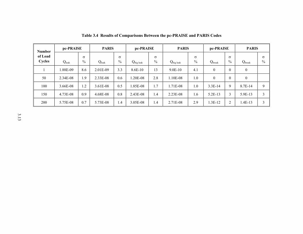
Table 3.4 Results o
pc-PRAISE PARIS
f en t -PR E and P S es
IS pc-PRAISE PARIS
Comparisons Betwe
pc-PRAISE
he pc AIS
PAR
ARI Cod
Numof LoCyc
σ%
σ% Q
σ%
ber ad
les Qleak σ % Qleak
Qbig leak
big leak
σ % Qbreak
σ % Qbreak
1 3. 9.0 4. 1.88E-09 8.6 2.01E-09 3 8.6E-10 13 E-10 1 0 0 0
50 0. 2. .1 1.0 0 0 0 2.34E-08 1.9 2.33E-08 6 1.20E-08 8 1 0E-08
10 0. 1. .7 1. 14 9 0 3.66E-08 1.2 3.61E-08 5 1.85E-08 7 1 1E-08 0 3.3E-14 9 8.7E-
150 0. 1. .2 1. 3 4.73E-08 0.9 4.68E-08 8 2.43E-08 4 2 3E-08 6 5.2E-13 3 5.9E-13
200 1. 1. .71E-08 2.9 1.3E-12 2 1.4E-13 3 5.75E-08 0.7 5.73E-08 4 3.05E-08 4 2
3.13
3.5.4 Effect of Sustained Primary Stress Level on Failure Probabilities
Parametric calculations of this report focus on pipe leak probabilities, with the objective to relate these leak probabilities to the cyclic stresses that cause preexisting cracks in a weld to grow to through-wall depths. The level of primary stress acting on the cracked pipe (used as input to the net section collapse calculation) was held constant in the parametric calculations. In all cases, the assigned primary stress levels were sufficiently low to have only a secondary effect on calculated leak probabilities. Neverthe-less, in some cases (very deep flaws), the sustained primary stresses can induce unstable crack growth for part-through flaws resulting in the simulation of sudden leaks. In this discussion, the primary stress is defined as the sum of the axial stresses caused by internal pressure, dead weight, and seismic bending moments. The stress caused by thermal-expansion bending moments is not included as part of the primary stress. Sensitivity calculations were performed to determine the effect of relatively high levels of primary stress on calculated leak probabilities. These calculations were for the same 6-in. (152-mm) Schedule 120 stainless pipe addressed by other sensitivity calculations.
tially constant leve ted operating life of the piping system.
he second transient simulated a fatigue stress at a rate of 5 cycles per year with the stress level adjusted provide a range of Q-factors. The input to pc-PRAISE for the pipe dead-weight stress was adjusted to
simulate the desired levels of primary stress.
s as characteri ter Q. Typical examples of the results are shown in
igure 3.8 for five levels of primary stress (8, 16, 24, 32, and 43 ksi [55, 110, 165, 220, and 296 MPa]). or the baseline case (8 ksi [55 MPa] primary stress) the break probability is 3 to 4 orders of magnitude
the e
.5.5 Effect of Abnormal/Seismic Stress Level on Failure Probabilities
The above calculations assumed that the cracked pipe experiences the specified primary stress as a continuous or sustained load. In many cases (as for seismic events), the maximum value of primary stress is not a sustained stress. A potential pipe failure must await the actual occurrence of the event. The above calculations would therefore overestimate leak and break probabilities for two reasons:
Two loading conditions were modeled in the pc-PRAISE calculations. The first simulated an essen
l of primary stress that was sustained over the simulaTto
Table 3.5 relates leak and rupture probabilities to the primary stress levels and to the cyclic stress level
zed by the fatigue crack growth parameFFless than the leak probability. Increasing the primary stress increases both the leak and break probabilities, but with a much larger effect on the break probabilities. The net effect is to diminish the difference between the two probabilities as shown in Table 3.5. For the very high primary stress of 43 ksi (296 MPa), the leak and break probabilities have virtuallysame magnitude. This limiting level of applied primary stress approaches the average flow stress of thpipe material, with the result being that even relatively small cracks can cause limit load failures of the pipe. In this situation, the pipe fails because of unstable crack extension such that a leak and a break occur at the same time. 3
3.14

Table 3.5 Fatigue Crack Growth Parameter Q = αN(∆σ)4 and Estimated Leak and Break Probabilities
Total Axial Stress, MPa (ksi)
Q 8 (55) 16 (110) 24 (165) 32 (220) 43 (296) 1 PL = 1.51E-05
PB = 2.67E-08 PL = 2.38E-05 PB = 3.04E-07
PL = 3.94E-05 PB = 5.49E-06
PL = 4.67E-03 PB = 4.64E-04
PL = 5.15E-01 PB = 5.15E-01
10 PL = 1.21E-04 PB = 9.43E-08
PL = 2.02E-04 PB = 8.15E-07
PL = 4.01E-4 PB = 9.46E-06
PL = 5.40E-03 PB = 4.82E-3
PL = 5.17E-01 PB = 5.16E-01
100 PL = 3.97E-03 PB = 4.48E-07
PL = 8.01E-03 PB = 3.84E-06
PL = 1.46E-02 PB = 3.37E-05
PL = 2.79E-02 PB = 5.69E-03
PL = 5.36E-01 PB = 5.29E-01
1000 PL = 1.06E-01 PB = 3.96E-06
PL = 1.62E-01 PB = 2.87E-05
PL = 2.19E-01 PB = 2.11E-04
PL = 2.78E-01 PB = 1.02E-02
PL = 6.85E-01 PB = 6.08E-01
10,000 PL = 5.53E-01 PB = 5.30E-05
PL = 6.40E-01 PB = 5.72E-04
PL = 7.07E-01 PB = 5.17E-03
PL = 7.59E-01 PB = 9.75E-02
PL = 9.08E-01 PB = 8.22E-01
) The calculations do not account for the low probability that the event will actually occur even once
(2) The event t life span, at which time the cracked
pipe is in its most severely degraded state.
manner. The 40-year cumulative failure probabilities (treated now as conditional failure probabilities given that the
f the
ese calculations, the abnormal stress (e.g., from a seismic event) was also cluded in the stress history that pc-PRAISE considered along with the fatigue crack growth analysis.
Q parameter increases with time) for various abnormal stress levels. The robabilities are conditional that the particular abnormal event occurs at the given value of Q (or time).
(1over the life span of the component
is unlikely to occur at the very end of the componen
The results of Figure 3.8 could be applied to abnormal/seismic events in an approximate
primary stress occurs) could be multiplied by the probability that the event occurs at least one time over the 40-year period. Such a calculation would still be conservative. It would account for the first otwo issues, but would not address the second issue related to exact time at which the event occurs. The sensitivity calculations described below address this second issue. To evaluate the effects of abnormal loadings, an extensive set of PFM calculations was performed with pc-PRAISE. As part of thinConsistent with the methodology of pc-PRAISE, the abnormal stress history was converted to an equivalent constant amplitude stress history of a selected number of cycles. After the simulated occurrence of the postulated abnormal stress, the crack size was returned to its size before the event. Figure 3.9 can be interpreted as cumulative leak probabilities versus time over 40 years versus time (i.e., it is implied that thepThe sustained contribution to the primary stress was held constant at 8 ksi (55 MPa). The leak probabilities of Figure 3.9 consider levels of sustained primary stress plus abnormal primary stress equal to 16 and 24 ksi (110 and 165 MPa) for which the results are very close to those for the same level of purely sustained primary stress.
3.15

Figure 3.8 The Effect of Sustained Primary (Axial) Stress on Leak Probability with Crack
Growth Parameter = αN(∆σ)4 (1 ksi = 6.9 MPa)
Figure 3.9 The Effect of Crack Growth Parameter = αN(∆σ)4 and the Abnormal Stress on the
Leak Probability (1 ksi = 6.9 MPa)
3.16

Figure 3.10 compares the results for a sustained primary stress of 24 ksi (165 MPa) with the results for an bnormal stress plus the sustained primary stress of 24 ksi (165 MPa) (with only 8 ksi [55 MPa] of this
total being of the sustained category). The leak probabilities for a sustained axial stress of 24 ksi (165 MPa) are somewhat higher than those for an abnormal stress of 16 ksi plus 8 ksi (110 MPa plus 55 MPa) of sustained primary stress. The maximum ratio of these leak probabilities is about 3. In conclusion, it appears that the results of the parametric calculations can be applied in an approximate manner to address the effects of low probability abnormal/seismic stresses. The sensitivity calculations show that it is conservative to use the results for the relevant level of primary stress (treated as a sustained stress), provided that these failure probabilities are multiplied by the probability that the event corresponding to the abnormal stress will occur over the life span of the component.
a
Figure 3.10 Comparison Between the Peak Probability for a Sustained Primary Stress of 24 ksi
(165 MPa) and Abnormal Plus Primary Stress of 24 ksi (165 MPa) with Crack Growth Parameter = αN(∆σ)4 (1 ksi = 6.9 MPa)
3.5.6 Effect of Leak Detection on Failure Probabilities
The parametric calculations of this report have simulated and thereby taken credit for the effects of leak detection (assuming relatively sensitive levels of leak detection) as a measure that can reduce the probabilities of both pipe breaks and of large leaks. However, it is important to note that leak detection can have no effect on the calculated “small leak” probabilities, because pc-PRAISE defines a “small leak” as any through-wall crack, even if the leakage from the crack is essentially zero. This section describes sensitivity calculations that evaluate the effects of a wide range of leak-detection thresholds on calculated pipe break probabilities.
3.17
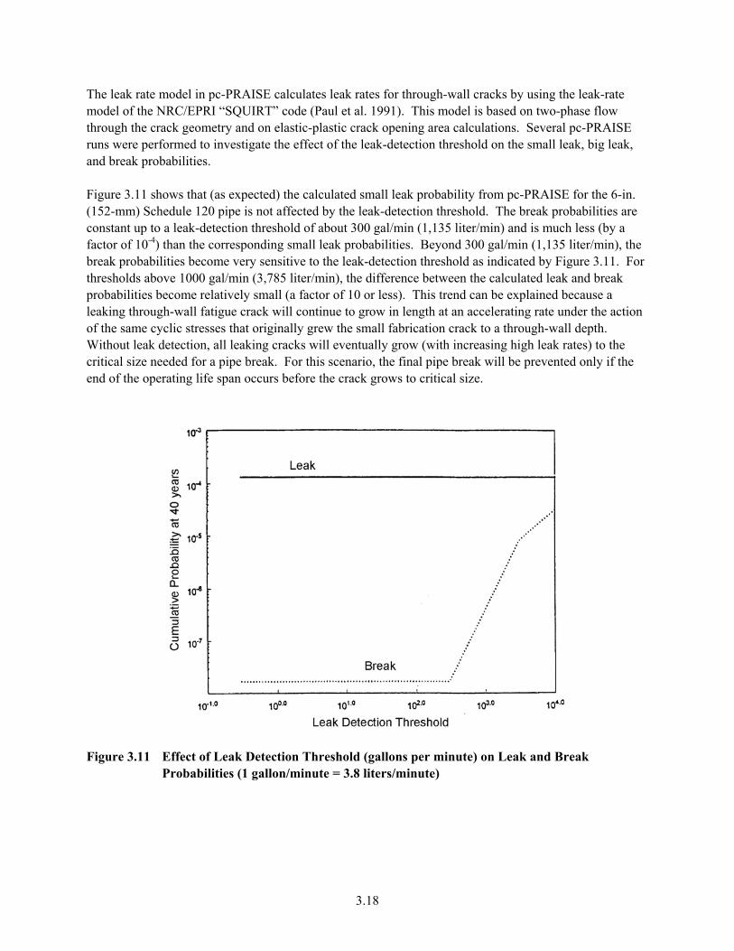
The leak rate model in pc y using the leak-rate model of the NRC/EPRI “ U phase flow through the crack geometry and on elastic-plastic crack opening area calculations. Several pc-PRAISE
vestigate the effect of the leak-detection threshold on the small leak, big leak,
he
f the same cyclic stresses that originally grew the small fabrication crack to a through-wall depth.
e
-PRAISE calculates leak rates for through-wall cracks bSQ IRT” code (Paul et al. 1991). This model is based on two-
runs were performed to inand break probabilities. Figure 3.11 shows that (as expected) the calculated small leak probability from pc-PRAISE for the 6-in.(152-mm) Schedule 120 pipe is not affected by the leak-detection threshold. The break probabilities are constant up to a leak-detection threshold of about 300 gal/min (1,135 liter/min) and is much less (by a factor of 10-4) than the corresponding small leak probabilities. Beyond 300 gal/min (1,135 liter/min), tbreak probabilities become very sensitive to the leak-detection threshold as indicated by Figure 3.11. Forthresholds above 1000 gal/min (3,785 liter/min), the difference between the calculated leak and break probabilities become relatively small (a factor of 10 or less). This trend can be explained because a leaking through-wall fatigue crack will continue to grow in length at an accelerating rate under the actionoWithout leak detection, all leaking cracks will eventually grow (with increasing high leak rates) to thcritical size needed for a pipe break. For this scenario, the final pipe break will be prevented only if the end of the operating life span occurs before the crack grows to critical size.
ure 3.11 Effect of Leak Detection Threshold (gallons per minute) on Leak and Break Probabilities (1 gallon/minute = 3.8 liters/minute)
Fig
3.18
3
Thipro ated for large number of welds and fittings without performing detailed Monte Carlo simulations for each
co cal, fabfrac Sen -wall streconsupcor r given Q-f ak probabilities, whereas other alculations have shown that longer flaws significantly increase pipe-break probabilities. Pipe failures are
mproand The sensitivity calculations indicate that pipe leak probabilities can be sensitive to the sustained primary tress (as opposed to cyclic stresses), but only when the primary stresses are a large fraction of the flow
ststre par Leaben nsensitive to the leak-detection threshold for typical leak-
etection capabilities. The threshold is important only if the leak-detection capability can detect only v
.6 Summary and Conclusions
s section has described a piping-reliability model and a method for predicting leak and break babilities in a structured parametric format. The approach permits piping reliability to be estim
amponent of interest. The model uses a fatigue crack growth model to grow pre-existing, semi-elliptirication defects. Critical flaw sizes for pipe breaks are based on a net section collapse criteria of ture.
sitivity studies have been performed for various combinations of uniform tension and throughss gradients caused by (1) discontinuity bending stresses, (2) radial thermal gradients, and (3) stress centrations. Calculated leak probabilities were found to be sensitive to the different types of erimposed through-wall stress gradients and local stress concentrations. The parametric curves responding to uniform tension can be used as an upper bound to estimate leak probabilities foactor values. The lengths of initial flaws have little effect on small le
core likely to be in the form of breaks when the corresponding leak probabilities and these break
babilities are relatively small because the initial flaws that result in pipe failures are both very deep very long.
sress of the pipe material. These calculations also show that the effects of potentially high primary
sses caused by low probability abnormal/seismic events can be estimated using the results of theametric calculations.
k detection can significantly reduce probabilities of pipe breaks and large leaks. The potential efits of leak detection are relatively i
dery large rates of leakage.
3.19

3.20
4 Fatigue of Stainless Steel Piping
4.1 Introduction
This section presents resul tric c alternative inspection strategies fail ties for s steel pi med in these calculations that the f nism s fatig growth f g fabricatio s located at or near rface rential The resu ped to guid lection of
service ection captrategies should ensure reliable detection of degradation before through-wall cracks result in leaks, and
y provi obabilities. The overall objective was to generate a ase loping risk-informed inservice inspection plans. Section 5 of
ipe sizes and cyclic stress levels. In each case, the probabilistic model simulated fatigue crack growth
from fabrication cracks in circumferential welds of as-built piping systems. The calculations addressed e full operating life of the components and simulated the detection of
resulting prevention of piping failures due to timely repairs.
eated as surface breaking flaws at the inner surface of the pipe. Fatigue crack initiation caused by cyclic s w
• The cyclic fatigue stresses corresponded to Q-factors that ranged from 1.0 to values as large as 106. For low values of Q-factors, the calculations predlarge initial flaws (50 percent of wall or greater). For the highest values of Q-factors, even relatively
f wall or less) could grow to become through-wall cracks before the end of The levels of cyclic stresses for the very high Q-factors were clearly outside
n codes (ASME Section III). These cases ection programs in that the stresses
that have often occurred during plant pipe-cracking incidents.
ts eure probabili
of param alculations that predict the effects of on reducing stainles ping. It is assuailure mecha of concern i ue crack rom pre-existin n flaw the inner sustrategies with suitable flaw-det
of circumfe welds. abilities and inspection frequencies. The selected
lts were develo e the seinsthereb de desired reductions in piping-failure prbroad b of data suitable for use in devethis report presents results of calculations that predict stress-corrosion cracking of stainless steel piping. Calculations were performed with the pc-PRAISE computer code using the technical approach and
rocedures described in Section 3. A large range of parameters was addressed to cover a broad sample ofpp
th the growing cracks along with the
4.2 Scope of Calculations
The calculations of this section were based on a number of modeling assumptions and addressed a rangeof parameters as follows: It was assumed that all failures were associated with weld fabrication flaws, which were conservatively trstresse as not addressed. • The pipe sizes ranged in wall thickness from 0.25 to 2.5 in. (6.35 to 63.5 mm)
icted very little fatigue crack growth even for very
small flaws (10 percent othe 40-year service life. the range of the cyclic stresses acceptable to piping desigare nevertheless of interest to the development of inservice inspcorrespond to unanticipated loadings, such as thermal fatigue, operation and have been the cause of
4.1
• All parametric calculations in this section assumed a simple uniform distribution of tensile stress through the thickness of the pipe wall. The effects of through-wall stress gradients can be estimatedby using an effective value of uniform tension. Sensitivity calculations described in Section 3 provide a basis for selecting suitable values for this effective value of uniform tensile stress.
• The simulations of inspection strategies focused on pipe leakage (i.e., through-wall cracks) as the
failure mode of most concern to inspection rather than pipe breaks. The implied assumption was that
to piping integrity. In this regard, calculations of leak probabilities involve fewer uncertainties than calculations of pipe-break probabilities and are less sensitive to certain poorly definleak-detection thresholds, and occurrence frequencies for design-limiting loads. However, it should
that the growth of cracks to through-wall depths is a precursor event to pipe breaks. Therefore, the prevention of pipe leaks can also serve as a useful surrogate measure for the effect ions to prevent pipe breaks.
• The calculatipiping system or for leak probabilities. Primary stresses were included in the calculations, but were assigned relatively
e cumulative failure probabilities at 40 years (end-of-life). While the pc-PRAISE code calculates failure probabilities corresponded to each year
ent
ctor itself can be interpreted as a surrogate for time.
• The calculations address inservice inspections by ultrasonic NDE performed on a periodic basis. with
h,
• All calculations take credit for leak detection and assume a relatively sensitive leak-detection threshol robabilities of large leaks and pipe breaks, but had no effect on small-leak probabilities.
• The calculati ress featu ect effect of
correlated versus independent pr of flaw ring a seq riodic inspections.
• The calculatio ze the benefits of each in ategy in ter ingle parameter
“improvement factor.” The improvement factor is the ratio of failure probability without inspection to the failure probability with inspection. No inspection (or a totally ineffective inspection) corresponds to an improvement factor of 1.0. In this report, we will assume that a relatively effective
the primary goal of inspection programs is to prevent leaks, with leak prevention considered to be an important element that is part of a defense-in-depth approach
ed inputs, such as flaw-length distributions,
be recognized
iveness of given inservice inspect
ons of leak probabilities were not intended to study the effects of primary stresses in s, which are a major factor for pipe-break probabilities, but are a secondary fact
low values consistent with the relative low-stress primary stress levels for most locations within piping systems.
• Results of calculations are reported in terms of th
throughout the plant operating life, it was not the intent to address aging effects or time-dependfailure rates in detail. Nevertheless, the presentations of results (i.e., cumulative failure probability versus Q-factor) can provide insight into time-dependent effects because the Q-fa
Each inspection strategy corresponds to a given probability of detection (POD) curve associated a given schedule of inspection intervals. It was assumed that all detected flaws are repaired. As sucthe calculations did not address the effects of flaw-sizing errors and flaw-acceptance criteria.
d of 3 gal/min (11.3 liter/min). This assumption had an effect only on calculated p
ons also add some important obabilities
res of the inspdetection du
ion model, such as theuence of pe
ns characteri spection str ms of a s
4.2
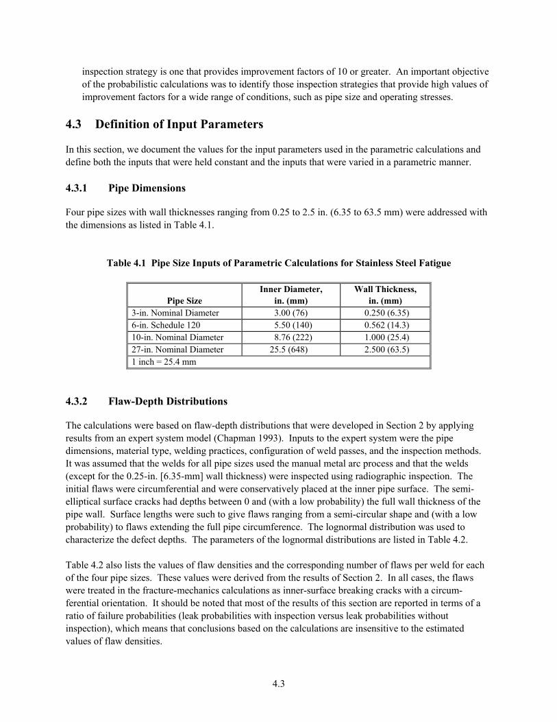
inspection strategy is one that provides improveof the probabilistic calculat
ment factors of 10 or greater. An important objective ions was to identify those inspection strategies that provide high values of
and .
.3.1 Pipe Dimensions
improvement factors for a wide range of conditions, such as pipe size and operating stresses. 4.3 Definition of Input Parameters
In this section, we document the values for the input parameters used in the parametric calculations define both the inputs that were held constant and the inputs that were varied in a parametric manner 4
Four pipe sizes with wall thicknesses ranging from 0.25 to 2.5 in. (6.35 to 63.5 mm) were addressed withthe dimensions as listed in Table 4.1.
Table 4.1 Pipe Size Inputs of Parametric Calculations for Stainless Steel Fatigue
Pipe Size Inner Diameter,
in. (mm) Wall Thickness,
in. (mm) 3-in. Nominal Diameter 3.00 (76) 0.250 (6.35) 6-in. Schedule 120 5.50 (140) 0.562 (14.3) 10-in. Nominal Diameter 8.76 (222) 1.000 (25.4) 27-in. Nominal Diameter 25.5 (648) 2.500 (63.5) 1 inch = 25.4 mm
4 Flaw-Depth Distributions .3.2
were developed in Section 2 by applying sults from an 1993). Inputs to the expert system were the pipe
imensions, material type, welding practices, configuration of weld passes, and the inspection methods.
e
e
able 4.2 also lists the values of flaw densities and the corresponding number of flaws per weld for each owerfere lts of this section are reported in terms of a
tio of failure probabilities (leak probabilities with inspection versus leak probabilities without which means that conclusions based on the calculations are insensitive to the estimated
values of flaw densities.
The calculations were based on flaw-depth distributions that re an expert system model (ChapmdIt was assumed that the welds for all pipe sizes used the manual metal arc process and that the welds (except for the 0.25-in. [6.35-mm] wall thickness) were inspected using radiographic inspection. Thinitial flaws were circumferential and were conservatively placed at the inner pipe surface. The semi-elliptical surface cracks had depths between 0 and (with a low probability) the full wall thickness of thpipe wall. Surface lengths were such to give flaws ranging from a semi-circular shape and (with a low probability) to flaws extending the full pipe circumference. The lognormal distribution was used to characterize the defect depths. The parameters of the lognormal distributions are listed in Table 4.2. T
f the four pipe sizes. These values were derived from the results of Section 2. In all cases, the flaws e treated in the fracture-mechanics calculations as inner-surface breaking cracks with a circum-ntial orientation. It should be noted that most of the resu
rainspection),
4.3
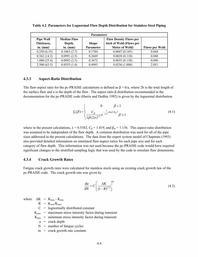
Table 4.2 Parameters for Lognormal Flaw Depth Distribution for Stainless Steel Piping
Parameters Pipe Wall Median Flaw Flaw Density Flaws per
Thickness, in. (mm)
Depth, in. (mm)
Shape Parameter
Inch of Weld (Flaws per Meter of Weld) Flaws per Weld
0.250 (6.35) 0.1063 (2.7) 0.1784 0.0047 (0.185) 0.044 0.562 (14.3) 0.0991 (2.5) 0.2669 0.0028 (0.110) 0.048 1.000 (25.4) 0.0892 (2.3) 0.3672 0.0035 (0.138) 0.096 2.500 (63.5) 0.0555 (1.4) 0.4993 0.0256 (1.008) 2.051
4.3.3 Aspect-Ratio Distribution
The flaw-aspect ratio for the pc-PRAISE calculations is defined as β = b/a, where 2b is the total length of the surface flaw and a is the depth of the flaw. The aspect ratio β distribution recommended in the
ocumentation for the pc-PRAISE code (Harris and Dedhia 1992) is given bd y the lognormal distribution
22
1 (ln / )0 21/2
0 1β <⎧⎪ ( )
1(2 )
mf Ce
β ββ λβ
βλβ π
−= ⎨≥⎪
⎩
(4.1)
where in the present calcul .5382, Cβ d 1.136 is aspect-ratio distribution was assumed to be indepen law depth. common ibutio s used for all of the pipe izes addressed in the present calculations. The data from the expert system model of Chapman (1993) lso provided detailed information on simulated flaw-aspect ratios for each pipe size and for each
-PRAISE code would have required e code to simulate flaw dimensions.
ting crack growth law of the -P was given by
ations, λ = 0 = 1.419, an βm = str
. Thdent of the f A di n wa
sacategory of flaw depth. This information was not used because the pcsignificant changes to the stratified sampling logic that was used by th 4.3.4 Crack Growth Rates
Fatigue crack growth rates were calculated for stainless steels using an exispc RAISE code. The crack growth rate
1/2(1 )
mda KCdN R
⎡ ⎤∆= ⎢ ⎥−⎣ ⎦
(4.2)
here ∆K = K - K
K = maximum stress intensity factor during transient
nsient a = crack depth
N = number of fatigue cycles m = crack growth rate constant.
w max min
R = Kmin/Kmax C = lognormally distributed constant
max
Kmin = minimum stress intensity factor during tra
4.4
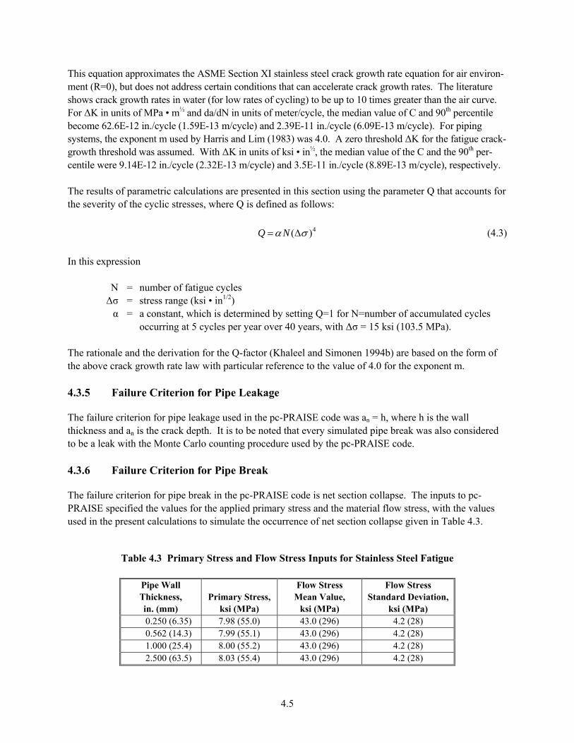
This eq ion approximates the ASME Section XI stainless stuat eel crack growth rate equation for air environ-ment (R=0), but does not address certain conditions that can accelerate crack growth rates. The literature
.
unts for
shows crack growth rates in water (for low rates of cycling) to be up to 10 times greater than the air curve. For ∆K in units of MPa • m½ and da/dN in units of meter/cycle, the median value of C and 90th percentile become 62.6E-12 in./cycle (1.59E-13 m/cycle) and 2.39E-11 in./cycle (6.09E-13 m/cycle). For piping systems, the exponent m used by Harris and Lim (1983) was 4.0. A zero threshold ∆K for the fatigue crack-growth threshold was assumed. With ∆K in units of ksi • in½, the median value of the C and the 90th per-centile were 9.14E-12 in./cycle (2.32E-13 m/cycle) and 3.5E-11 in./cycle (8.89E-13 m/cycle), respectively The results of parametric calculations are presented in this section using the parameter Q that accothe severity of the cyclic stresses, where Q is defined as follows:
4( )Q Nα σ= ∆ (4.3)
In this expression N = number of fatigue cycles ∆σ = stress range (ksi • in1/2) α = a constant, which is determined by setting Q=1 for N=number of accumulated cycles
occurring at 5 cycles per year over 40 years, with ∆σ = 15 ksi (103.5 MPa). The rationale and the derivation for the Q-factor (Khaleel and Simonen 1994b) are based on the form of the above crack growth rate law with particular reference to the value of 4.0 for the exponent m. 4.3.5 Failure Criterion for Pipe Leakage
The failure criterion for pipe leakage used in the pc-PRAISE code was an = h, where h is the wall thickness and an is the crack depth. It is to be noted that every simulated pipe break was also considered to be a leak with the Monte Carlo counting procedure used by the pc-PRAISE code. .3.6 Failure Criterion for Pipe Break
RAISE spec primary stress and the material flow stress, with the values sed in the present calculations to simulate the occurrence of net section collapse given in Table 4.3.
4
The failure criterion for pipe break in the pc-PRAISE code is net section collapse. The inputs to pc-ified the values for the applied P
u
Table 4.3 Primary Stress and Flow Stress Inputs for Stainless Steel Fatigue
Pipe Wall Thickness, in. (mm)
Primary Stress, ksi (MPa)
Flow Stress Mean Value,
ksi (MPa)
Flow Stress Standard Deviation,
ksi (MPa) 0.250 (6.35) 7.98 (55.0) 43.0 (296) 4.2 (28) 0.562 (14.3) 7.99 (55.1) 43.0 (296) 4.2 (28) 1.000 (25.4) 8.00 (55.2) 43.0 (296) 4.2 (28) 2.500 (63.5) 8.03 (55.4) 43.0 (296) 4.2 (28)
4.5
4.4 Probability of Detection Curves
The evaluations of alternative inspection strategies addressed a range of probability of detection (POD) curves for ultrasonic examination of stainless steel piping. The approach was to establish POD curves
at represented widely differing levels of NDE performance. Individual curves were intended to bound e probability of detection levels expected from inspection teams performing inservice inspections of
piping at plants in the field. To establish POD curves, n informal expert judgment elicitation was erformed using staff at PNNL with specialized knowledge of NDE performance data from piping-
ns.
was recognized that a population of inspection teams operating under field conditions can exhibit a onsiderable range of POD performance, even though all such teams meet minimum code requirements
timating POD curves for the present calculations was that the better teams had passed the ASME Section XI Appendix VIII performance
o
ert judgment also considered information and trends bserved in the PNNL round robin studies on UT inspection of wrought stainless steel piping with wall
thth
apinspection round robins and from recent industry efforts in the area of NDE performance demonstratio
Itcfor inspecting nuclear piping systems. The basic premise in es
demonstration. ASME Section XI requires a minimum of 10 flaws and 20 blanks to be examined andrequires a failing grade for either of the following: (1) more than two false calls or (2) the team fails tdetect at least 8 of the 10 flaws. The informal expothicknesses of 0.60 to 1.0 in. (15.2 to 25.4 mm) (Bates et al. 1987; Heasler et al. 1990). The NDE experts at PNNL were asked to define POD curves by estimating parameters for the POD function used in the pc-PRAISE code:
( )
( )
ND1P ( ) 12
erfc / *
A
A A
ε ε
ν
= + −
= ⎡ ⎤⎣ ⎦
(4.4)
A = area of the crack
ter ν is 1.6. Several POD curves
om PNNL studies were reviewed, and it was determined that a value of ν = 1.6 was consistent with ublished curves. While the assigned value of the slope parameter ν was held constant, the actual slope
of the plotted curves becomes steeper for better POD curves. Thus, the slope was implicitly correlated to the detection threshold parameter A*. The value of ε was assigned to ensure that smaller values of ε also correspond to smaller values of A*. Three POD curves were selected: • Marginal Performance: A team with a POD performance that is described by this curve would have
only a small chance of passing an Appendix VIII performance demonstration, and its performance would not be representative of current day capabilities.
where PND = probability of nondetection = 1 - POD
A* = area of crack for 50% PND ε = smallest possible PND for very large cracks ν = “slope” of the PND curve. Based on measured performance levels for PNNL’s mini round-robin teams (Heasler et al. 1990; Heasler and Doctor 1996), a range of estimates for A* (crack area for 50% POD) was provided by the NDEexperts. Harris, Dedhia, and Lu (1992) assumed that the “slope” paramefrp
4.6
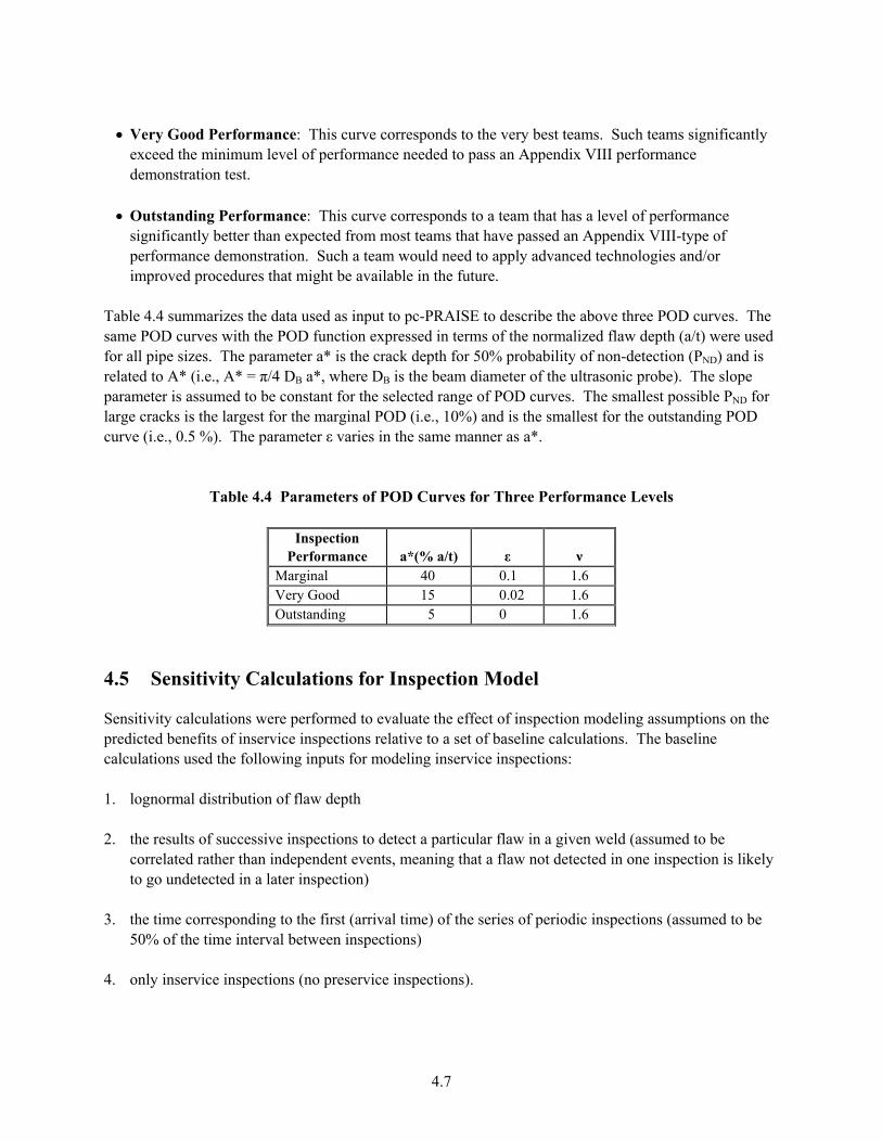
• Very Good Performance: This curve corresponds to the very best teams. Such teams significantly
exceed the minimum level of performance needed to pass an Appendix VIII performance demonstration test.
• Outstanding Performance: This curve corresponds to a team that has a level of performance
significantly better than expected from most teams that have passed an Appendix VIII-type of performance demonstration. Such a team would need to apply advanced technologies and/or improved procedures that might be available in the future.
Table 4.4 summarizes the data used as input to pc-PRAISE to describe the above three POD curves. The same POD curves with the POD function expressed in terms of the normalized flaw depth (a/t) were used for all pipe sizes. The parameter a* is the crack depth for 50% probability of non-detection (PND) and is related to A* (i.e., A* = π/4 DB a*, where DB is the beam diameter of the ultrasonic probe). The slope parameter is assumed to be constant for the selected range of POD curves. The smallest possible PND for large cracks is the largest for the marginal POD (i.e., 10%) and is the smallest for the outstanding POD curve (i.e., 0.5 %). The parameter ε varies in the same manner as a*.
n Performance a*(% a/t) ε ν
Table 4.4 Parameters of POD Curves for Three Performance Levels
Inspectio
Marginal 40 0.1 1.6 Very Good 15 0.02 1.6 Outstanding 5 0 1.6
4.5 Sensitivity Calculations for Inspection Model
Sensitivity calculations were performed to evaluate the effect of inspection modeling assumptions on the predicted benefits of inservice inspections relative to a set of baseline calculations. The baseline calculations used the following inputs for modeling inservice inspections: 1. lognormal distribution of flaw depth 2. the results of successive inspections to detect a particular flaw in a given weld (assumed to be
correlated rather than independent events, meaning that a flaw not detected in one inspection is likely to go undetected in a later inspection)
3. the time corresponding to the first (arrival time) of the series of periodic inspections (assumed to be
50% of the time interval between inspections) 4. only inservice inspections (no preservice inspections).
4.7
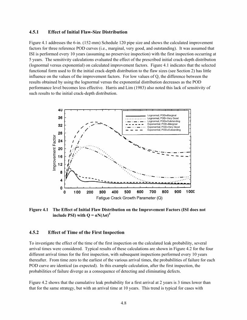
4.5.1 Effect of Initial Flaw-Size Distribution
Figure 4.1 addresses the 6-in. (152-mm) Schedule 120 pipe size and shows the calculated improvement factors for three reference POD curves (i.e., marginal, very good, and outstanding). It was assumed that ISI is performed every 10 years (assuming no preservice inspection) with the first inspection occurring at 5 years. The sensitivity calculations evaluated the effect of the prescribed initial crack-depth distribution (lognormal versus exponential) on calculated improvement factors. Figure 4.1 indicates that the selected functional form used to fit the initial crack-depth distribution to the flaw sizes (see Section 2) has little influence on the values of the improvement factors. For low values of Q, the difference between the results obtained by using the lognormal versus the exponential distribution decreases as the POD performance level becomes less effective. Harris and Lim (1983) also noted this lack of sensitivity of such results to the initial crack-depth distribution.
Figure 4.1 The Effect of Initial Flaw Distribution on the Improvement Factors (ISI does not
include PSI) with Q = αN(∆σ)4
4.5.2 Effect of Time of the First Inspection
To investigate the effect of the time of the first inspection on the calculated leak probability, several arrival times were considered. Typical results of these calculations are shown in Figure 4.2 for the four different arrival times for the first inspection, with subsequent inspections performed every 10 years thereafter. From time zero to the earliest of the various arrival times, the probabilities of failure for each POD curve are identical (as expected). In this example calculation, after the first inspection, the probabilities of failure diverge as a consequence of detecting and eliminating defects. Figure 4.2 shows that the cumulative leak probability for a first arrival at 2 years is 3 times lower than that for the same strategy, but with an arrival time at 10 years. This trend is typical for cases with
4.8
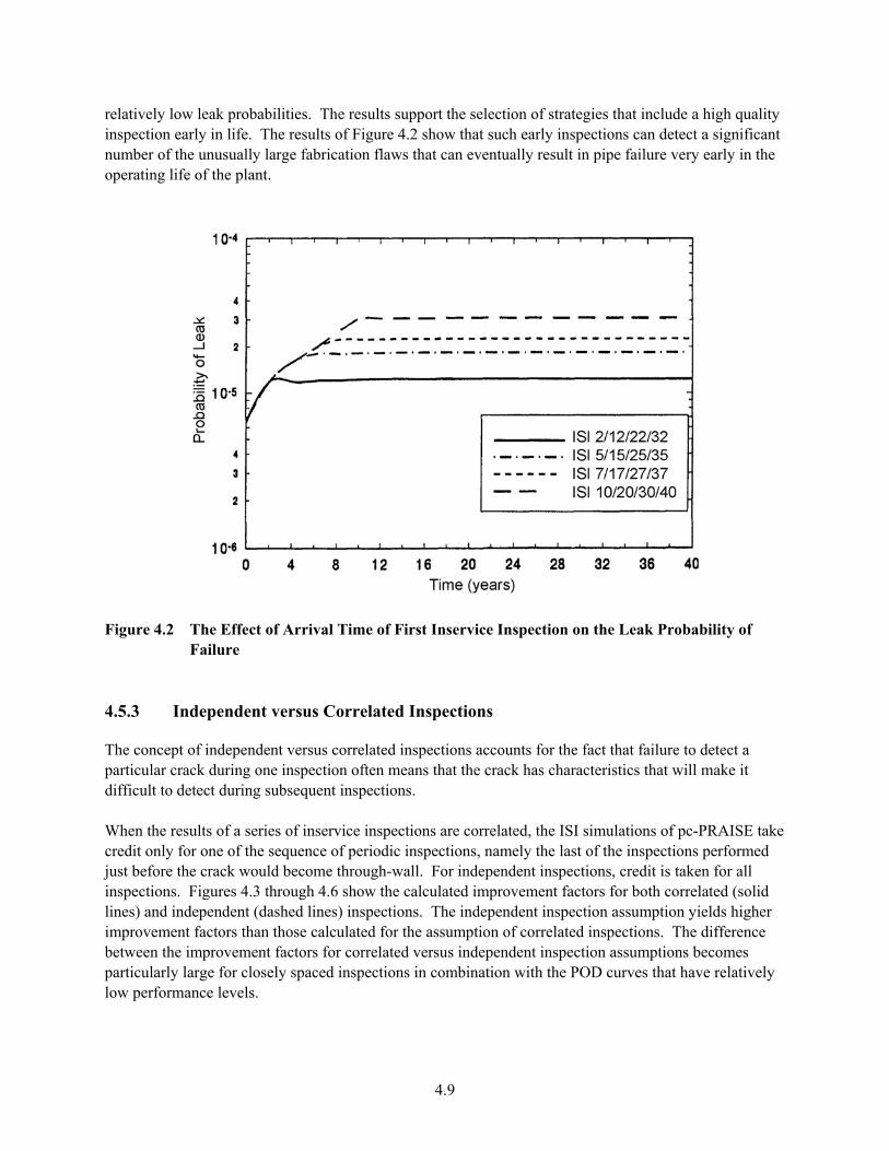
relatively low leak probabilities. The results support the selection of strategies that include a high quality inspection early in life. The results of Figure 4.2 show that such early inspections can detect a significant number of the unusually large fabrication flaws that can eventually result in pipe failure very early in the operating life of the plant.
Figure 4.2 The Effect of Arrival Time of First Inservice Inspection on the Leak Probability of
Failure 4.5.3 Independent versus Correlated Inspections
The concept of independent versus correlated inspections accounts for the fact that failure to detect a particular crack during one inspection often means that the crack has characteristics that will make it difficult to detect during subsequent inspections. When the results of a series of inservice inspections are correlated, the ISI simulations of pc-PRAISE tcredit only for one of the sequence of periodic inspections, namely the last of the inspections performed just before the crack would become through-wall. For independent inspections, credit is taken for ainspections. Figures 4.3 through 4.6 show the calculated improvement factors for both correlated (lines) and independent (dashed lines) inspections. The independent inspection assumption yields higimprovement factors than those calculated for the assumption of correlated inspections. The difference
etween the improvement factors for correlated versus independent inspection assumptions becomes
ake
ll solid
her
large for closely spaced inspections in combination with the POD curves that have relatively low performance levels.
bparticularly
4.9
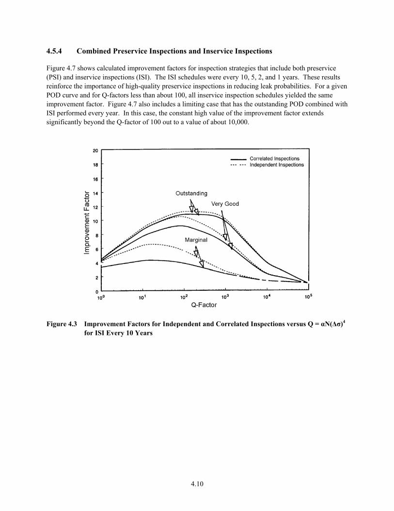
4.5.4 Combined Preservice Inspections and Inservice Inspections
ce
n
Figure 4.7 shows calculated improvement factors for inspection strategies that include both preservi(PSI) and inservice inspections (ISI). The ISI schedules were every 10, 5, 2, and 1 years. These results reinforce the importance of high-quality preservice inspections in reducing leak probabilities. For a givePOD curve and for Q-factors less than about 100, all inservice inspection schedules yielded the same improvement factor. Figure 4.7 also includes a limiting case that has the outstanding POD combined withISI performed every year. In this case, the constant high value of the improvement factor extends significantly beyond the Q-factor of 100 out to a value of about 10,000.
Improvement Facto
igure 4.3 rs for Independent and Correlated Inspections versus Q = αN(∆σ)4 for ISI Every 10 Years
F
4.10

Figure 4.4 Improvement Factors for Independent and Correlated Inspections versus Q = αN(∆
for ISI Every 5 Years σ)4
Figure 4.5 Improvement Factors for Independent and Correlated Inspections versus Q = αN(∆σ)4
for ISI Every 2 Years
4.11
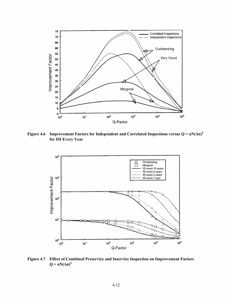
mprovement Factors for Independent and Correlated Inspections versus Q = αN(∆σ)4
or ISI Every Year Figure 4.6 I
f
igure 4.7 Effect of Combined Preservice and Inservice F Inspection on Improvement Factors Q = αN(∆σ)4
4.12
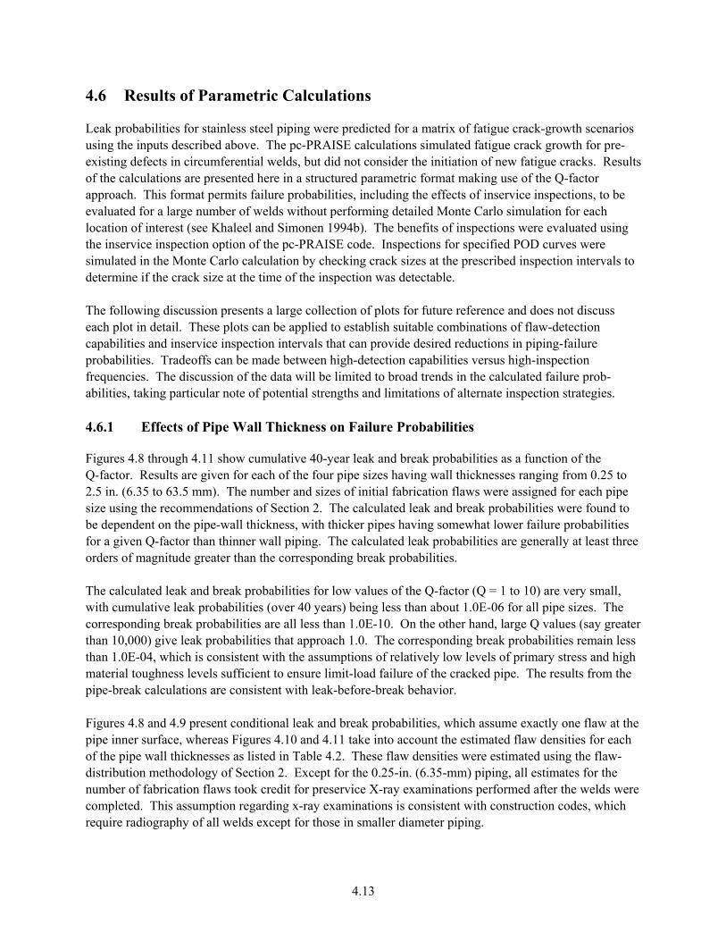
4.6 Results of Parametric Calculations
Leak probabilities for stainless steel piping were predicted for a matrix of fatigue crack-growth scenarios using the inputs described above. The pc-PRAISE calculations simulated fatigue crack growth for pre-existing defects in circumferential welds, but did not consider the initiation of new fatigue cracks. Resuof the calculations are presented here in a structured parametric format making use of the Q-factor approach. This format permits failure probabilities, including the effects of inservice inspections, to be evaluated for a large number of welds without performing detailed Monte Carlo simulation for each location of in
lts
terest (see Khaleel and Simonen 1994b). The benefits of inspections were evaluated using e inservice inspection option of the pc-PRAISE code. Inspections for specified POD curves were
cribed inspection intervals to determine if the crack size at the time of the inspection was detectable.
be limited to broad trends in the calculated failure prob-bilities, taking particular note of potential strengths and limitations of alternate inspection strategies.
cknesses ranging from 0.25 to
2.5 in. (6.35 to 63.5 mm). The number and sizes of initial fabrication flaws were assigned for each pipe ize using the recommendations of Section 2. The calculated leak and break probabilities were found to
s for a given Q- e orders of mag
he calculated leak and break probabilities for low values of the Q-factor (Q = 1 to 10) are very small, with cumulative leak probabilities (over 40 years) being less than about 1.0E-06 for all pipe sizes. The corresponding break probabilities are all less than 1.0E-10. On the other hand, large Q values (say greater than 10,000) give leak probabilities that approach 1.0. The corresponding break probabilities remain less than 1.0E-04, which is consistent with the assumptions of relatively low levels of primary stress and high material toughness levels sufficient to ensure limit-load failure of the cracked pipe. The results from the pipe-break calculations are consistent with leak-before-break behavior. Figures 4.8 and 4.9 present conditional leak and break probabilities, which assume exactly one flaw at the pipe inner surface, whereas Figures 4.10 and 4.11 take into account the estimated flaw densities for each of the pipe wall thicknesses as listed in Table 4.2. These flaw densities were estimated using the flaw-distribution methodology of Section 2. Except for the 0.25-in. (6.35-mm) piping, all estimates for the number of fabrication flaws took credit for preservice X-ray examinations performed after the welds were completed. This assumption regarding x-ray examinations is consistent with construction codes, which require radiography of all welds except for those in smaller diameter piping.
thsimulated in the Monte Carlo calculation by checking crack sizes at the pres
The following discussion presents a large collection of plots for future reference and does not discuss each plot in detail. These plots can be applied to establish suitable combinations of flaw-detection capabilities and inservice inspection intervals that can provide desired reductions in piping-failure probabilities. Tradeoffs can be made between high-detection capabilities versus high-inspection frequencies. The discussion of the data willa 4.6.1 Effects of Pipe Wall Thickness on Failure Probabilities
Figures 4.8 through 4.11 show cumulative 40-year leak and break probabilities as a function of theQ-factor. Results are given for each of the four pipe sizes having wall thi
sbe dependent on the pipe-wall thickness, with thicker pipes having somewhat lower failure probabilitie
factor than thinner wall piping. The calculated leak probabilities are generally at least threnitude greater than the corresponding break probabilities.
T
4.13
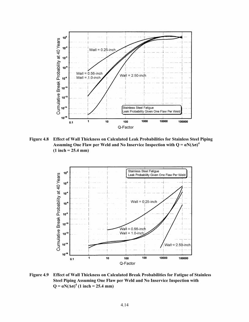
Figure 4.8 ffect of Wall Thickness on Calculated Leak Probabilities for Stainless Steel Piping
ssuming One Flaw per Weld and No Inservice Inspection with Q = αN(∆σ)4 1 inch = 25.4 mm)
EA(
igure 4.9 Effect of Wall Thickness on Calculated Break Probabilities for Fatigue of Stainless Steel Piping Assuming One Flaw per Weld and No Inservice Inspection with Q = αN(∆σ)4 (1 inch = 25.4 mm)
F
4.14
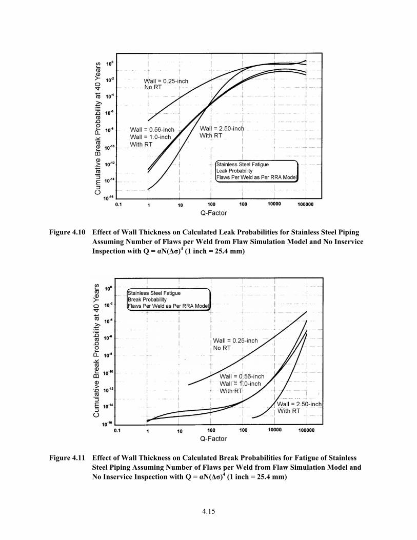
Figure 4.10 Effect of Wall Thickness on Calculated Leak Probabilities for Stainless Steel Piping
Assuming Number of Flaws per Weld from Flaw Simulation Model and No Inservice Inspection with Q = αN(∆σ)4 (1 inch = 25.4 mm)
Figure 4.11 Effect of Wall Thickness on Calculated Break Probabilities for Fatigue of Stainless
Steel Piping Assuming Number of Flaws per Weld from Flaw Simulation Model and No Inservice Inspection with Q = αN(∆σ)4 (1 inch = 25.4 mm)
4.15
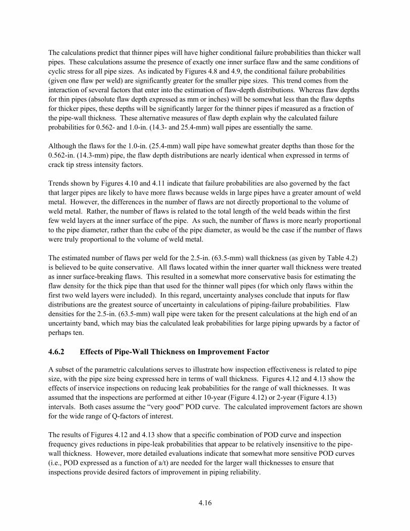
The calculations predict that thinner pipes will have higher conditional failure probabilities than thicker wall pipes. These calculations assume the presence of exactly one inner surface flaw and the same conditions of cyclic stress for all pipe sizes. As indicated by Figures 4.8 and 4.9, the conditional failure probabilities (given one flaw per weld) are significantly greater for the smaller pipe sizes. This trend comes from the interaction of several factors that enter into the estimation of flaw-depth distributions. Whereas flaw depths for thin pipes (absolute flaw depth expressed as mm or inches) will be somewhat less than the flaw depths for thicker pipes, these depths will be significantly larger for the thinner pipes if measured as a fraction of the pipe-wall thickness. These alternative measures of flaw depth explain why the calculated failure probabilities for 0.562- and 1.0-in. (14.3- and 25.4-mm) wall pipes are essentially the same. Although the flaws for the 1.0-in. (25.4-mm) wall pipe have somewhat greater depths than those for the 0.562-in. (14.3-mm) pipe, the flaw depth distributions are nearly identical when expressed in terms of crack tip stress intensity factors. Trends shown by Figures 4.10 and 4.11 indicate that failure probabilities are also governed by the fact that larger pipes are likely to have more flaws because welds in large pipes have a greater amount of weld metal. However, the differences in the number of flaws are not directly proportional to the volume of weld metal. Rather, the number of flaws is related to the total length of the weld beads within the first
w weld layers at the inner surface of the pipe. As such, the number of flaws is more nearly proportional s
po
he estimated num y Table 4.2) believed to be quite conservative. All flaws located within the inner quarter wall thickness were treated
ce-breaking flaws. This resulted in a somewhat more conservative basis for estimating the aw density for the thick pipe than that used for the thinner wall pipes (for which only flaws within the
edensities for the ncertainty band
4.6.2 Effects of Pipe-Wall Thickness on Improvement Factor
A subset of the parametric calculations serves to illustrate how inspection effectiveness is related to pipe size, with the pipe size being expressed here in terms of wall thickness. Figures 4.12 and 4.13 show the effects of inservice inspections on reducing leak probabilities for the range of wall thicknesses. It was assumed that the inspections are performed at either 10-year (Figure 4.12) or 2-year (Figure 4.13) intervals. Both cases assume the “very good” POD curve. The calculated improvement factors are shown for the wide range of Q-factors of interest. The results of Figures 4.12 and 4.13 show that a specific combination of POD curve and inspection frequency gives reductions in pipe-leak probabilities that appear to be relatively insensitive to the pipe-wall thickness. However, more detailed evaluations indicate that somewhat more sensitive POD curves (i.e., POD expressed as a function of a/t) are needed for the larger wall thicknesses to ensure that inspections provide desired factors of improvement in piping reliability.
feto the pipe diameter, rather than the cube of the pipe diameter, as would be the case if the number of flawwere truly pro rtional to the volume of weld metal.
ber of flaws per weld for the 2.5-in. (63.5-mm) wall thickness (as given bTisas inner surfaflfirst two weld layers were included). In this regard, uncertainty analyses conclude that inputs for flaw distributions ar the greatest source of uncertainty in calculations of piping-failure probabilities. Flaw
2.5-in. (63.5-mm) wall pipe were taken for the present calculations at the high end of an, which may bias the calculated leak probabilities for large piping upwards by a factor of u
perhaps ten.
4.16
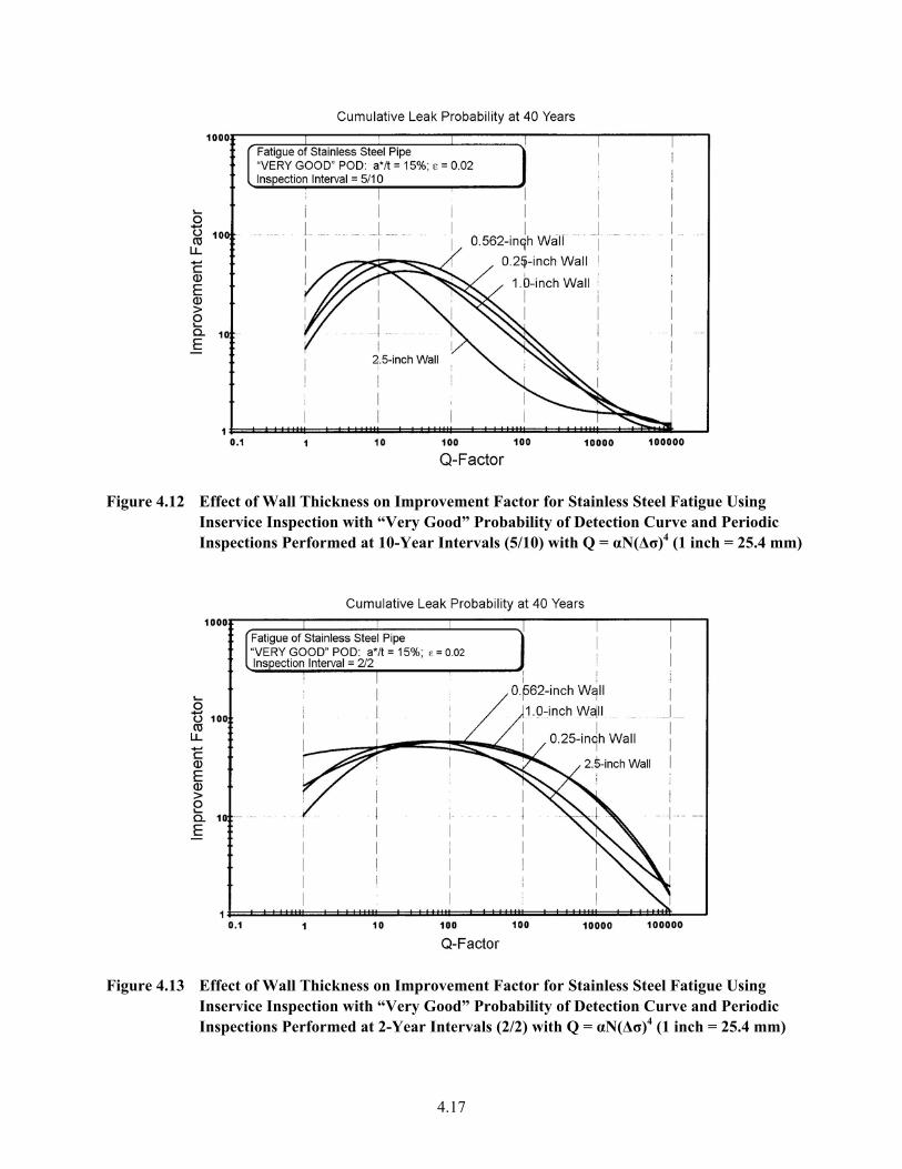
nIn )
Figure 4.12 Effect of Wall Thickness on Improvement Factor for Stainless Steel Fatigue Using I service Inspection with “Very Good” Probability of Detection Curve and Periodic
spections Performed at 10-Year Intervals (5/10) with Q = αN(∆σ)4 (1 inch = 25.4 mm
Figure 4.13 Effect of Wall Thickness on Improvement Factor for Stainless Steel Fatigue Using
Inservice Inspection with “Very Good” Probability of Detection Curve and Periodic Inspections Performed at 2-Year Intervals (2/2) with Q = αN(∆σ)4 (1 inch = 25.4 mm)
4.17
4.6.3 Improvement Factors for Various Pipe-Wall Thicknesses
Figures 4.14 through 4.18 give improvement factors for the four pipe-wall thicknesses ranging from 0.25 to 2.5 in. (6.35 to 63.5 mm) and give calculated factors for the “marginal,” “very good,” and “outstanding” POD curves. The inspection intervals range from 1 year to 10 years. The collection of plots is organized in the following manner: • Figures 4.14a, 4.14b, and 4.14c are for the stainless steel piping with a wall thickness of 0.25 in.
(6.35 mm). Factors of improvement in piping reliability for the “marginal,” “very good,” and “outstanding” POD curves are addressed by Figures 4.14a, 4.14b, and 4.14c respectively. Each of the individual curves on these figures corresponds to a different ISI interval (1, 2, 4, and 10 years).
• Figures 4.15a, 4.15b, and 4.15c are for the 0.562-in. (14.3-mm) wall stainless steel piping and cover
the same range of POD curves and inspection intervals as for the 0.25-in. (6.35-mm) wall piping. • Figures 4.16a, 4.16b, and 4.16c are for the 1.0-in. (25.4-mm) wall stainless steel piping and cover the
same range of POD curves and inspection intervals as for the other pipe sizes. • Figures 4.17a, 4.17b, and 4.17c are for the 2.5-in. (63.5-mm) wall stainless steel piping and cover the
same range of POD curves and inspection intervals as for the other pipe sizes.
Figure 4.14a Improvement Factor for Fatigue of 0.25-in. (6.35-mm) Wall Stainless Steel Piping
Using Inservice Inspection with “Marginal” Probability of Detection Curve and Periodic Inspections Performed at Various Intervals with Q = αN(∆σ)4
4.18

Improvement Factor for Fatigue of 0.25-in. (6.35-mm) Wall Stainless Steel PipingUsing Inservice Inspection with “Very Good” Probability of Detection C
Figure 4.14b urve and
Periodic Inspections Performed at Various Intervals with Q = αN(∆σ)4
Figure 4.14c Improvement Factor for Fatigue of 0.25-in. (6.35-mm) Wall Stainless Steel Piping
Using Inservice Inspection with “Outstanding” Probability of Detection Curve and Periodic Inspections Performed at Various Intervals with Q = αN(∆σ)4
4.19

Figure 4.15a Improvement Factor for Fatigue of 0.562-in. (14.3-mm) Wall Stainless Steel Pipin
Using Inservice Inspection with “Marginal” Probability of Detection Curve and Periodic Inspections Performed at Various Intervals with Q = αN(∆σ)4
g
igure 4.15b Improvement Factor for Fatigue of 0.562-in. (14.3-mm) Wall Stainless Steel Piping Using Inservice Inspection with “Very Good” Probability of Detection Curve and Periodic Inspections Performed at Various Intervals with Q = αN(∆σ)4
F
4.20
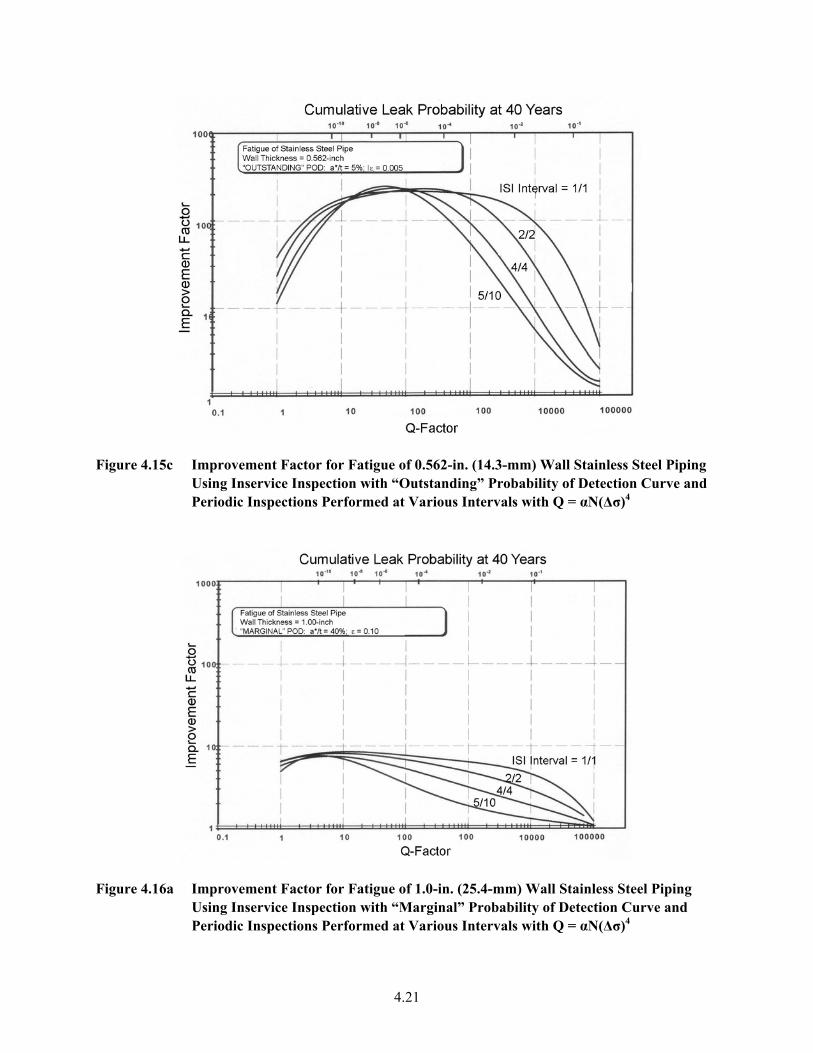
Figure 4.15c Improvement Factor for Fatigue of 0.562-in. (14.3-mm) Wall Stainless Steel Piping
Using Inservice Inspection with “Outstanding” Probability of Detection Curve and Periodic Inspections Performed at Various Intervals with Q = αN( σ)4 ∆
Figure 4.16a Improvement Factor for Fatigue of 1.0-in. (25.4-mm) Wall Stainless Steel Piping
Using Inservice Inspection with “Marginal” Probability of Detection Curve and Periodic Inspections Performed at Various Intervals with Q = αN(∆σ)4
4.21
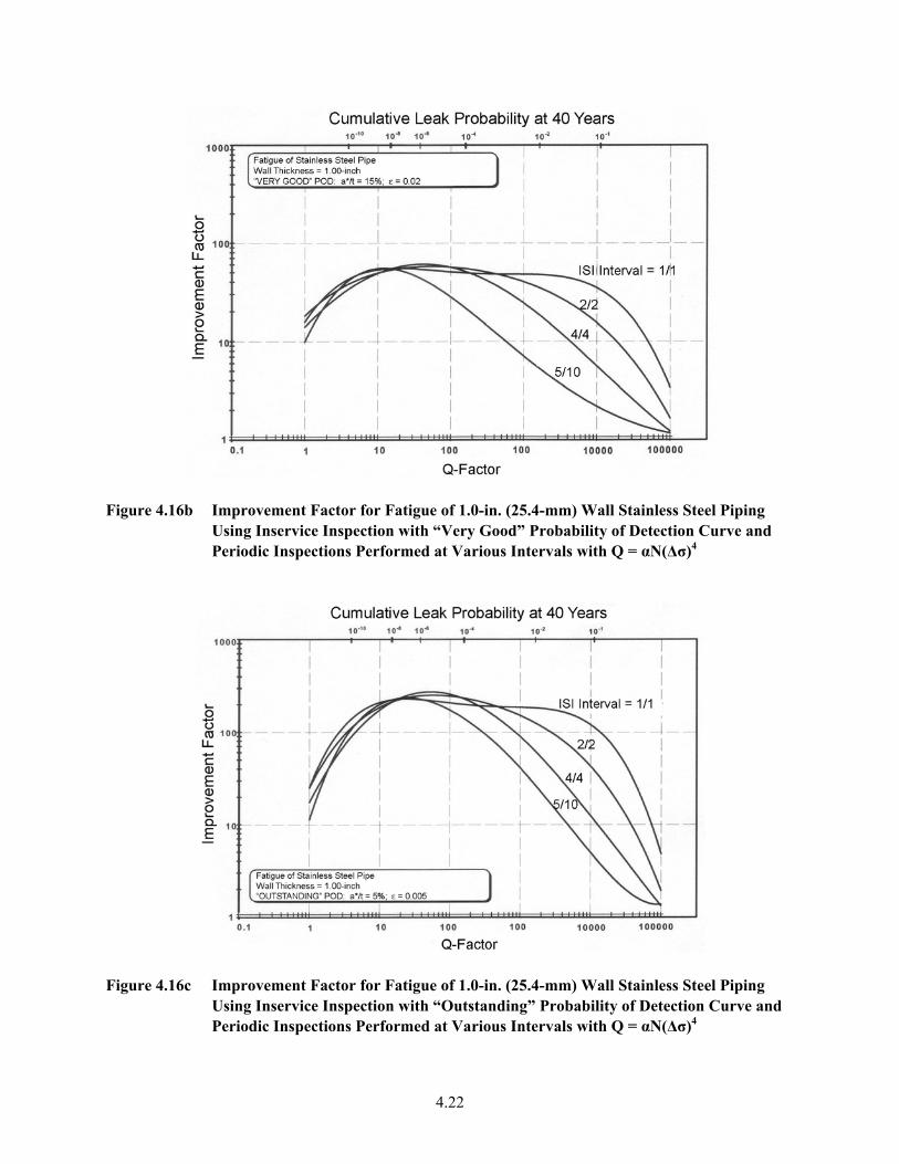
Figure 4.16b Improvement Factor for Fatigue of 1.0-in. (25.4-mm) Wall Stainless Steel Piping
Using Inservice Inspection with “Very Good” Probability of Detection Curve Periodic Inspections Performed at Various Intervals with Q = αN(∆σ 4
and )
ure 4.16c Improvement Factor for Fatigue of 1.0-in. (25.4-mm) Wall Stainless Steel Piping Using Inservice Inspection with “Outstanding” Probability of Detection Curve and Periodic Inspections Performed at Various Intervals with Q = αN(∆σ)4
Fig
4.22
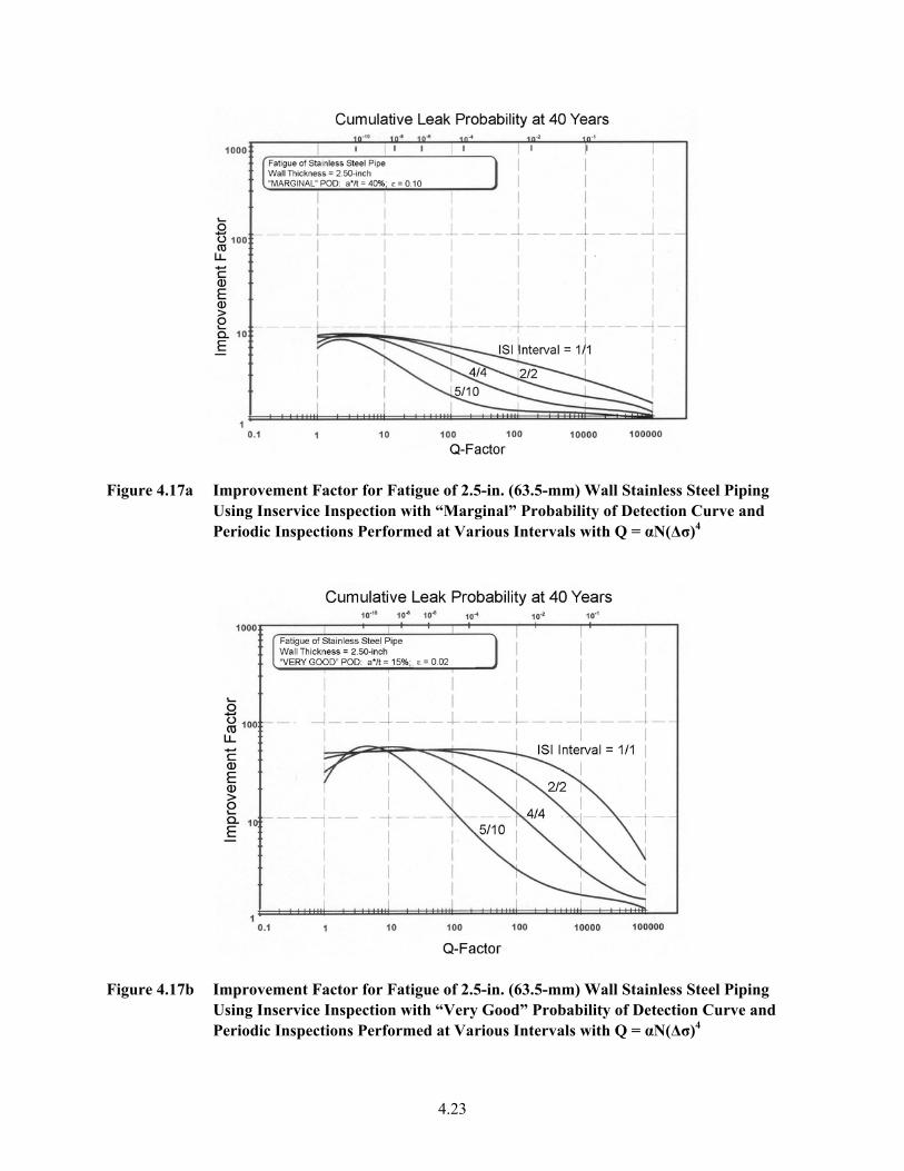
ure 4.17a Improvement Factor for Fatigue of 2.5-in. (63.5-mm) Wall Stainless Steel PipinUsing Inservice Inspection with “Marginal” Probability of Detection Curve andPeriodic Inspections Performed at Various Intervals with
Fig g
Q = αN(∆σ)4
Figure 4.17b Improvement Factor for Fatigue of 2.5-in. (63.5-mm) Wall Stainless Steel Piping
Using Inservice Inspection with “Very Good” Probability of Detection Curve anPeriodic Inspections Performed at Various Intervals with Q = αN(∆σ)4
d
4.23
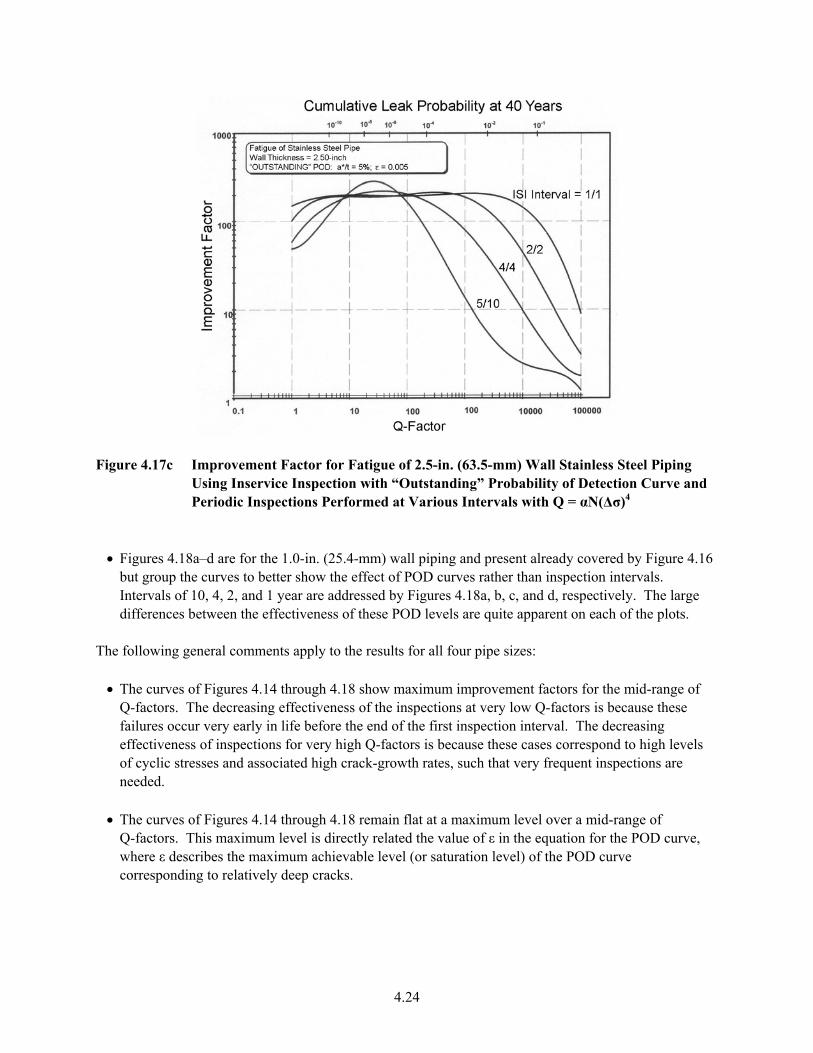
Figure 4.17c Improvement Factor for Fatigue of 2.5-in. (63.5-mm) Wall Stainless Steel Piping
Using Inservice Inspection with “Outstanding” Probability of Detection Curve and Periodic Inspections Performed at Various Intervals with Q = αN(∆σ)4
• Figures 4.18a–d are for the 1.0-in. (25.4-mm) wall piping and present already covered by Figure 4.16
but group the curves to better show the effect of POD curves rather than inspection intervals. Intervals of 10, 4, 2, and 1 year are addressed by Figures 4.18a, b, c, and d, respectively. The large differences between the effectiveness of these POD levels are quite apparent on each of the plots.
The following general comments apply to the results for all four pipe sizes: • The curves of Figures 4.14 through 4.18 show maximum improvement factors for the mid-range of
Q-factors. The decreasing effectiveness of the inspections at very low Q-factors is because these failures occur very early in life before the end of the first inspection interval. The decreasing effectiveness of inspections for very high Q-factors is because these cases correspond to high levels of cyclic stresses and associated high crack-growth rates, such that very frequent inspections are needed.
• The curves of Figures 4.14 through 4.18 remain flat at a maximum level over a mid-range of
Q-factors. This maximum level is directly related the value of ε in the equation for the POD curve, where ε describes the maximum achievable level (or saturation level) of the POD curve corresponding to relatively deep cracks.
4.24
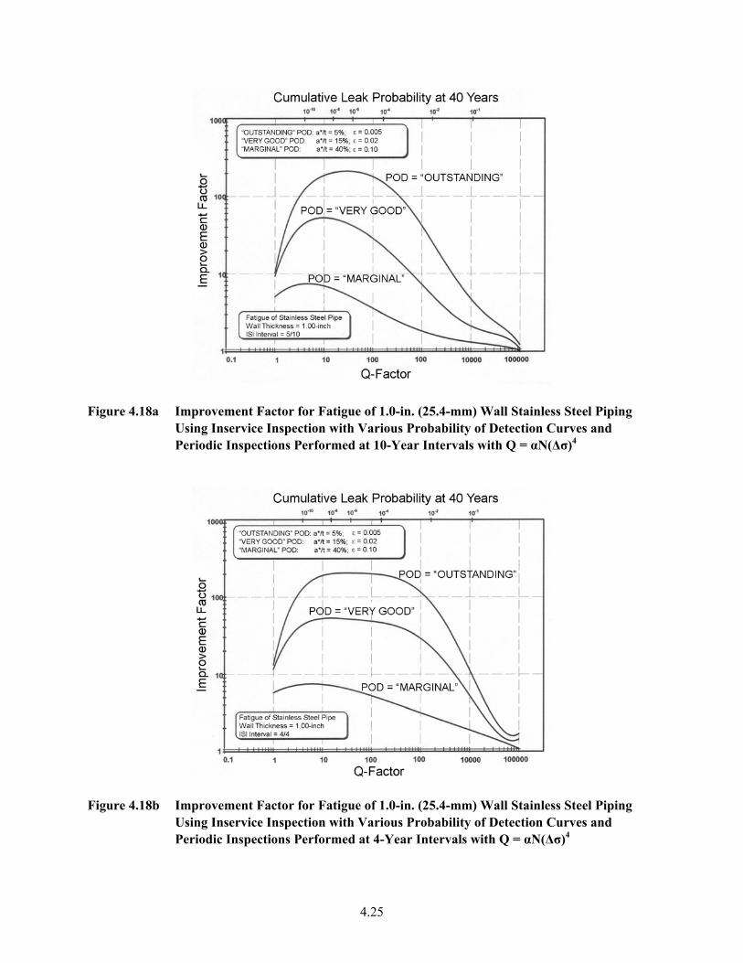
Figure 4.18a Improvement Factor for Fatigue of 1.0-in. (25.4-mm) Wall Stainless Steel Piping
Using Inservice Inspection with Various Probability of Detection Curves and Periodic Inspections Performed at 10-Year Intervals with Q = αN(∆σ)4
Figure 4.18b Improvement Factor for Fatigue of 1.0-in. (25.4-mm) Wall Stainless Steel Piping
Using Inservice Inspection with Various Probability of Detection Curves and Periodic Inspections Performed at 4-Year Intervals with Q = αN(∆σ)4
4.25
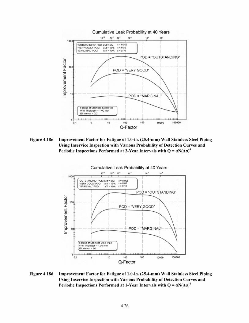
Figure 4.18c Improvement Factor for Fatigue of 1.0-in. (25.4-mm) Wall Stainless Steel Piping
Using Inservice Inspection with Various Probability of Detection Cur4ves and
Periodic Inspections Performed at 2-Year Intervals with Q = αN(∆σ)
Figure 4.18d Improvement Factor for Fatigue of 1.0-in. (25.4-mm) Wall Stainless Steel Piping
Using Inservice Inspect hion wit Various Probability of Detection Curves and Periodic Inspections Performed at 1-Year Intervals with Q = αN(∆σ)4
4.26
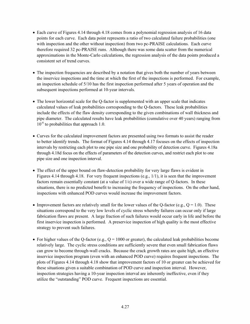
• Each curve of Figures 4.14 through 4.18 comes from a polynomial regression analysis of 16 data a r of tw lcu d failure probabilities (one
sp n e ith nspection) pc RA c s. uso e data scatter from the nu erical
nte-Carlo calculations, the regression analysis of the data points produced a consistent set of trend curves.
xample,
• The lower horizontal scale for the Q-factor is supplemented with an upper scale that indicates calculated values of leak probabilities correspondiinclude the effects of the flaw density corresponding to the given combinations of wall thickness and
om
• Curves for the calculated improvement factors are presented using two formats to assist the reader at of Figures 4.14 through 4.17 focuses on the effects of inspection
• The effect of the upper bound on flaw-detection probability forFigures 4.14 through 4.18. For very frequent inspections (e.gfactors remain essentially constant (at a value of 1/ε) over a wide range of Q-factors. In these
• Improvement factors are relatively small for the losituations correspond to the very low levels of cyclic stress whereby failures can occur only if large
the e
• For higher values of the Q-factor (e.g., Q = 1000 or greater), the calculated leak probabilities become fficiently severe that even small fabrication flaws
can grow to become through-wall cracks. Because the crack growth rates are quite high, an effective
d for of POD curve and inspection interval. However,
inspection strategies having a 10-year inspection interval are inherently ineffective, even if they utilize the “outstanding” POD curve. Frequent inspectio
points for each curve. Each data point represents atio o ca latewith in ectio and th other w out i from two
h there was -Pm
ISE cal ulation Each cm
rve therefore required 32 pc-PRAISE runs. Althougapproximations in the Mo
• The inspection frequencies are described by a notation that gives both the number of years between
the inservice inspections and the time at which the first of the inspections is performed. For ean inspection schedule of 5/10 has the first inspection performed after 5 years of operation and the subsequent inspections performed at 10-year intervals.
ng to the Q-factors. These leak probabilities
pipe diameter. The calculated results have leak probabilities (cumulative over 40 years) ranging fr10-6 to probabilities that approach 1.0.
to better identify trends. The formintervals by restricting each plot to one pipe size and one probability of detection curve. Figures 4.18a through 4.18d focus on the effects of parameters of the detection curves, and restrict each plot to one pipe size and one inspection interval.
very large flaws is evident in
., 1/1), it is seen that the improvement
situations, there is no predicted benefit to increasing the frequency of inspections. On the other hand,inspections with enhanced POD curves would increase the improvement factors.
wer values of the Q-factor (e.g., Q = 1.0). These
fabrication flaws are present. A large fraction of such failures would occur early in life and beforefirst inservice inspection is performed. A preservice inspection of high quality is the most effectivstrategy to prevent such failures.
relatively large. The cyclic stress conditions are su
inservice inspection program (even with an enhanced POD curve) requires frequent inspections. The plots of Figures 4.14 through 4.18 show that improvement factors of 10 or greater can be achievethese situations given a suitable combination
ns are essential.
4.27
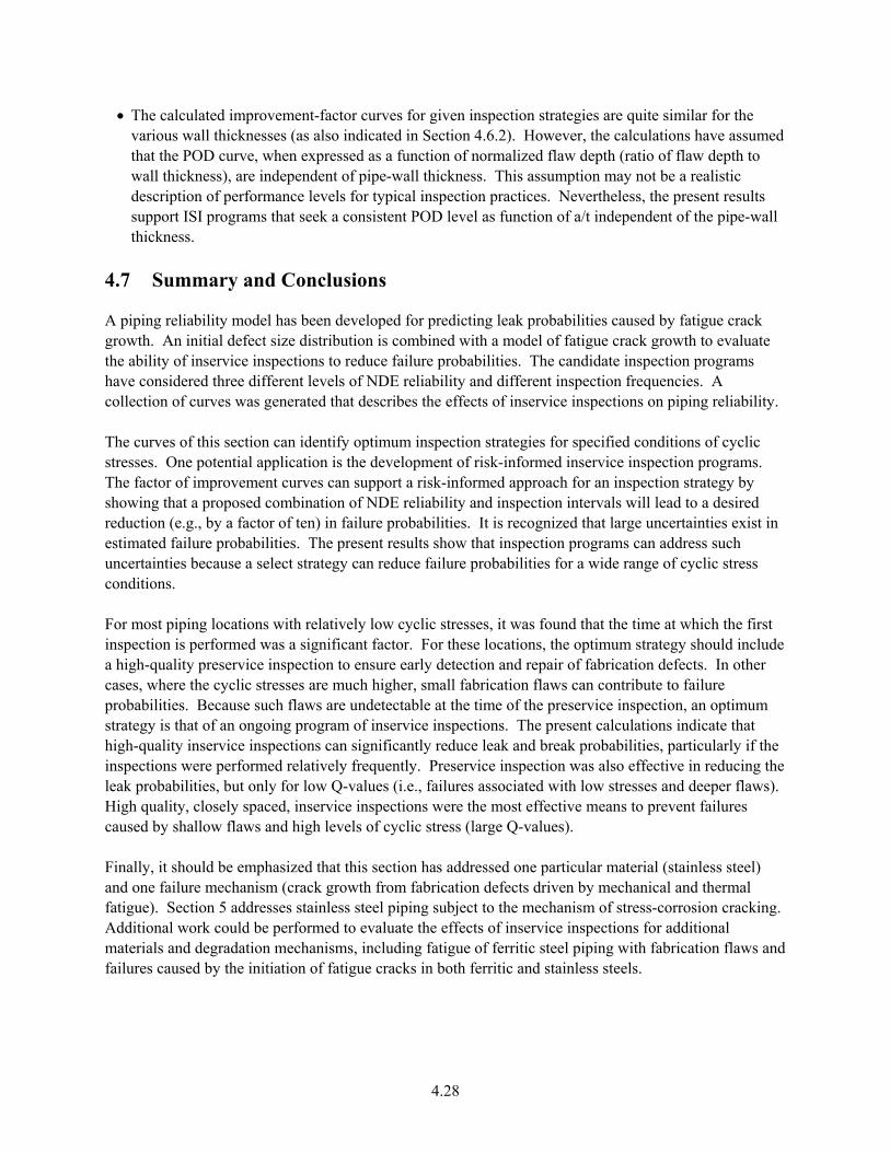
• The calculated improvement-factor curves for given inspection strategies are quite similar for the various wall thicknesses (as also indicated in Section 4.6.2). However, the calculations have assumed that the POD curve, when expressed as a function of normalized flaw depth (ratio of flaw depth to
-wall
Conclusions
ability.
he factor of improvement curves can support a risk-informed approach for an inspection strategy by
exist in
ge of cyclic stress onditions.
For most piping locations with relatively low cyclic stresses, it was found that the time at which the first
ervice inspection, an optimum trategy is that of an ongoing program of inservice inspections. The present calculations indicate that igh-quality inservice inspections can significantly respections were performed relatively frequently. Preservice inspection was also effective in reducing the
s).
el) nd one failure mechanism (crack growth from fabrication defects driven by mechanical and thermal
s steel piping subject to the mechanism of stress-corrosion cracking. Additional work could be performed to evaluate the effects of inservice inspections for additional
wall thickness), are independent of pipe-wall thickness. This assumption may not be a realistic description of performance levels for typical inspection practices. Nevertheless, the present results support ISI programs that seek a consistent POD level as function of a/t independent of the pipethickness.
4.7 Summary and
A piping reliability model has been developed for predicting leak probabilities caused by fatigue crack growth. An initial defect size distribution is combined with a model of fatigue crack growth to evaluate the ability of inservice inspections to reduce failure probabilities. The candidate inspection programs have considered three different levels of NDE reliability and different inspection frequencies. A collection of curves was generated that describes the effects of inservice inspections on piping reli The curves of this section can identify optimum inspection strategies for specified conditions of cyclicstresses. One potential application is the development of risk-informed inservice inspection programs. Tshowing that a proposed combination of NDE reliability and inspection intervals will lead to a desired reduction (e.g., by a factor of ten) in failure probabilities. It is recognized that large uncertainties estimated failure probabilities. The present results show that inspection programs can address such uncertainties because a select strategy can reduce failure probabilities for a wide ranc
inspection is performed was a significant factor. For these locations, the optimum strategy should include a high-quality preservice inspection to ensure early detection and repair of fabrication defects. In other cases, where the cyclic stresses are much higher, small fabrication flaws can contribute to failure probabilities. Because such flaws are undetectable at the time of the pressh duce leak and break probabilities, particularly if the inleak probabilities, but only for low Q-values (i.e., failures associated with low stresses and deeper flawHigh quality, closely spaced, inservice inspections were the most effective means to prevent failurescaused by shallow flaws and high levels of cyclic stress (large Q-values). Finally, it should be emphasized that this section has addressed one particular material (stainless steafatigue). Section 5 addresses stainles
materials and degradation mechanisms, including fatigue of ferritic steel piping with fabrication flaws and failures caused by the initiation of fatigue cracks in both ferritic and stainless steels.
4.28
5 Intergranular Stress Corrosion of Stainless Steel Piping
5.1 Introduction
This section describes probabilistic calculations that address intergranular stress-corrosion cracking (IGSCC) of stainless steel piping, a degradation mechanism of major concern to nuclear pressure boundary integrity. The objective was to simulate the cracking of stainless steel piping under IGSCC
rnate inspection strategies as a means to reduce failure probabilities. A range of pipe sizes and operating conditions was addressed by a matrix of parametric
ost
he present calculations build on past studies by the nuclear power industry (General Electric Company
s .
er evaluated effects of personnel, equipment, crack characteristics, and human factors. Trends f data from these studies were used in the work described below to develop input data for pc-PRAISE
or
nce.
f plant loading/unloading cycles in addition to adjustments to residual stress levels. The crack detection ata (POD curves) by use of the pc-PRAISE model are also described.
parametric approach was adopted in the present calculations to characterize IGSCC by a single damage
parameter. This parameter (Dσ) depends on residual nditions, and degree of sensiti trix of calculations to address a wide range of pipe sizes, mater , and servco loped. lts lcu nti cti ure ies tha with I st he ecti section presents conclusions reg venes ati to e e re B . 5. rros ck el
Th r stress-corrosio in redcrack initiation, a simulati row sm , an en e a
conditions and to evaluate the benefits of alte
calculations. The results permit the development of effective inservice inspection programs that are basedon tradeoffs between inspection frequencies and NDE sensitivities. The objective is to identify the meffective approaches to improving piping reliability. T1982a, 1982b) and NRC (Hazelton and Koo 1988), which have addressed both IGSCC causes and preventive actions. A critical issue has been the difficulty of using ultrasonic testing (UT) to detect IGSCC. PNNL’s past research on NDE reliability has included systematic studies to quantify NDE effectiveness. The first statistically based data for the probability of detection (POD) of IGSCC in weldof stainless steel piping were generated based on a piping inspection round robin (Doctor et al. 1983)The resulting data related POD to crack size and other important variables and covered the performance of several inspection teams participating in the round robin. Later work (Taylor et al. 1989; Heasler et al. 1990) furthofor characterizing the effectiveness of UT inspections in detecting IGSCC. The first part of this section describes the stress-corrosion cracking model used in the pc-PRAISE computer program (Harris 1981; Harris et al. 1986a; Harris et al. 1986b; Harris and Dedhia 1992) fsimulating the initiation and growth of IGSCC cracks. This model is based on laboratory data from IGSCC tests in combination with calibration of the model using field data from pipe-cracking experiePNNL has improved on the prior calibrations (Harris et al. 1986b) by making adjustments to the modelingod
Astresses, environment co
zation. A ma ials ice nditions was deve The resu of these ca lations qua fy the redu ons in fail probabilitt can be achieved various IS rategies. T final subs on of this arding ISI effecti s as a mitig on action nhance th liability of WR piping
2 Stress-Co ion Cra ing Mod
e probabilistic model of the pc-PRAISE code fo n cracking cludes a p iction of on of the g th of very all cracks d a treatm t of the tim nd
5.1
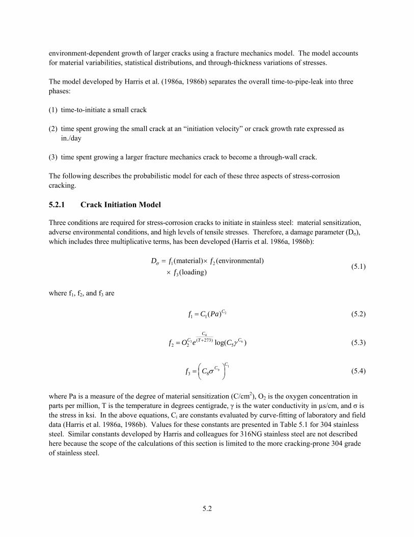
environment-dependent growth of larger cracks using a fracture mechanics model. The model accounts r material variabilities, statistical distributions, and through-thickness variations of stresses.
he model developed by Harris et al. (1986a, 1986b) separates the overall time-to-pipe-leak into three
ph (1) all c (2) g the small crack at an “initiation velocity” or crack growth rate expressed as
in./day
me a through-wall crack.
teel: material sensitization, dverse environmental conditions, and high levels of tensile stresses. Therefore, a damage parameter (Dσ),
here f , f , and f are
fo
Tases:
time-to-initiate a sm rack
time spent growin
(3) time spent growing a larger fracture mechanics crack to beco
The following describes the probabilistic model for each of these three aspects of stress-corrosion cracking. 5.2.1 Crack Initiation Model
Three conditions are required for stress-corrosion cracks to initiate in stainless sawhich includes three multiplicative terms, has been developed (Harris et al. 1986a, 1986b):
1 2
3
(material) (environmental)(loading)
D f ff
σ = ×
× (5.1)
w 1 2 3
2
1 1( )Cf C Pa= (5.2
)
4
3 6( 273)C
2 2 5log( )f O e CC CT γ+ )
here Pa is a measure of the degree of material sensitization (C/cm2), O is the oxygen concentration in
d
ibed
= (5.3
1
93 8
CCf C σ⎛ ⎞= ⎜ ⎟
⎝ ⎠ (5.4)
w 2
parts per million, T is the temperature in degrees centigrade, γ is the water conductivity in µs/cm, and σ is the stress in ksi. In the above equations, Ci are constants evaluated by curve-fitting of laboratory and fieldata (Harris et al. 1986a, 1986b). Values for these constants are presented in Table 5.1 for 304 stainless steel. Similar constants developed by Harris and colleagues for 316NG stainless steel are not descrhere because the scope of the calculations of this section is limited to the more cracking-prone 304 grade of stainless steel.
5.2
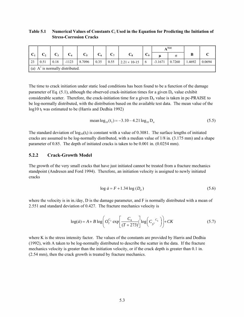
Table 5.1 Numerical Values of Constants Ci Used in the Equation for Predicting the Initiation ofStress-Corrosion Cracks
A1(a)
C1 C2 C3 C4 C5 C6 C7 C8 C9 µ σ B C
23 0.51 0.18 -1123 8.7096 0.35 0.55 2.21 × 10⁻¹⁵ 6 -3.1671 0.7260 1.4692 0.0694
(a) A1 is normally distributed.
The time to crack initiation under static load conditions has been found to be a function of the damage parameter of Eq. (5.1), although the observed crack-initiation times for a given Dσ value exhibit considerable scatter. Therefore, the crack-initiation time for a given Dσ value is taken in pc-PRAISE to
e log-normally distributed, with the distribution based on the available test data. The mean value of the log10 tI was estimated to be (Harris and Dedhia 1992)
b
10 I 10mean log (t ) 3.10 4.21 log Dσ= − − (5.5) The standard deviation of log10(tI) is constant with a value of 0.3081. The surface lengths of initiated cracks are assumed to be log-normally distributed, with a median value of 1/8 in. (3.175 mm) and a shape parameter of 0.85. The depth of initiated cracks is taken to be 0.001 in. (0.0254 mm). 5.2.2 Crack-Growth Model
The growth of the very small cracks that have just initiated cannot be treated from a fracture mechanics standpoint (Andresen and Ford 1994). Therefore, an initiation velocity is assigned to newly initiated cracks log 1.34 log ( )a F Dσ= +& (5.6)
n of 2.551 and sta
where the velocity is in in./day, D is the damage parameter, and F is normally distributed with a mea
ndard deviation of 0.427. The fracture mechanics velocity is
3 642 5
log( ) log exp log( 273)
C CCa A B O C CKT γ
⎛ ⎞⎡ ⎤ ⎛ ⎞= + +⎜ ⎟⎜ ⎟⎢ ⎥+ ⎝ ⎠⎣ ⎦⎝ ⎠& (5.7)
where K is th edhia 992), with uted to describe the scatter in the data. If the fracture echanics velocity is greater than the initiation velocity, or if the crack depth is greater than 0.1 in. .54 mm), then the crack growth is treated by fracture mechanics.
e stress intensity factor. The values of the constants are provided by Harris and DA taken to be log-normally distrib(1
m(2
5.3
5.2.3 Residual Stresses
Residual stresses influence both crack initiation and propagation. The damage parameter Dσ is a function of the stress, which consists of both the applied (service-induced pressure and thermal) and residual stresses. The crack-tip stress-intensity factor is ap resK K K= + (5.8)
where Kap and Kres are the stress-intensity factors attributable to the applied stress and residual stresses respectively. Data on welding residual stresses display large scatter (Harris et al. 1986b; Harris and Dedhia 1992) and differ significantly, depending on pipe size. The calculations reported here are concerned with the stress-corrosion cracking behavior of small pipes (OD = 4 to 10 in. [102 to 254 mm]), intermediate pipes (OD = 10 to 20 in. [254 to 508 mm]), and large pipes (OD > 20 in. [508 mm]). The present calculations are based on the pc-PRAISE default inputs for residual stresses, which are the values originally estimated by Harris et al. (1986b).
he local residual stresses at the inside surface of small and intermediate pipes are treated as being normally T cal
values samplinner surface Pa) with a standard deviation of 14.58 ksi (100 MPa). The independently sampled stress at the outside surface was 24.4 ksi (168 MPa) with a standard deviation of 14.47 ksi
8 MPa). For the intermediate pipe, the inner surface stress had a mean value of 9.3 ksi (64 MPa) and a i e
intermediate ksi (98 MPa).
arris and Dedhia (1992) document the default pc-PRAISE inputs in detail for the complex pattern of the inner surface had a mean tensile stress of 38 ksi
(262 MPa). The through-thickness variation in stress had compressive stresses developing within the
or ing equal to the material-flow stress. This criterion is
pplicable to high-toughness materials where failure occurs because of insufficient remaining cross-e applied loads. The criterion is expressed as
Tdistributed. he through-thickness distributions of stress are assumed to be linear variations between lo
ed for the inner and outer surfaces. For small pipes, the mean value of residual stress at the was 24.4 ksi (168 M
(9standard dev ation of 14.47 ksi (98 MPa). The independently sampled stress at the outer surface of th
pipe had a mean value of 9.3 ksi (64 MPa) with a standard deviation of 14.47 Hresidual stresses in large pipes. In summary,
inner quarter-wall thickness and changing again to tension stress at greater depths. 5.2.4 Failure Criterion for Pipe Breakage and Leakage
In this study, flaws can fail the pipe by either breakage (pipe rupture) or leakage. The failure criterion fpipe break was that of the net section stress becomasectional area to support th
Lc p flo p crackA (A -A )σ σ> (5.
In Equation (5.9), Ap is the pipe cross-sectional area, Acrack is the area of the crack, σflo is the material flow stress, and σLc is the axial component of load-controlled stress, which in pc-PRAISE is due to internal pressure and dead weight. The flow stress of the material σLc used in Equation (5.9) was taken to
9)
5.4
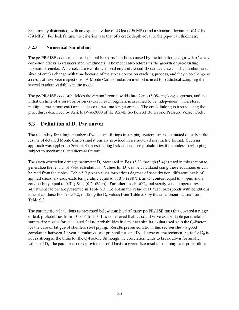
be normally distributed, with an expected value of 43 ksi (296 MPa) and a standard deviation of 4.2 ksi (29 MPa). For leak failure, the criterion was that of a crack depth equal to the pipe-wall thickness.
ess-
s. A Monte Carlo simulation method is used for statistical sampling the
everal random variables in the model.
e
he stress-corrosion damage parameter Dσ presented in Eqs. (5.1) through (5.4) is used in this section to σ can be calculated using
e read from the tables. Table 5.2 gives values for various degrees of sepplied stress, a steady-state temperature equal to 550°F (288°C), an O2 content equal to 8 ppm, and a
σ
σ obabilities.
5.2.5 Numerical Simulation
The pc-PRAISE code calculates leak and break probabilities caused by the initiation and growth of strcorrosion cracks in stainless steel weldments. The model also addresses the growth of pre-existing fabrication cracks. All cracks are two-dimensional circumferential ID surface cracks. The numbers and sizes of cracks change with time because of the stress-corrosion cracking process, and they also change asa result of inservice inspections The pc-PRAISE code subdivides the circumferential welds into 2-in.- (5.08-cm) long segments, and thinitiation time-of-stress-corrosion cracks in each segment is assumed to be independent. Therefore, multiple cracks may exist and coalesce to become longer cracks. The crack linking is treated using the procedures described by Article IWA-3000 of the ASME Section XI Boiler and Pressure Vessel Code. 5.3 Definition of Dσ Parameter
The reliability for a large number of welds and fittings in a piping system can be estimated quickly if the results of detailed Monte Carlo simulations are provided in a structured parametric format. Such an approach was applied in Section 4 for estimating leak and rupture probabilities for stainless steel piping subject to mechanical and thermal fatigue. Tgeneralize the results of PFM calculations. Values for D these equations or can b nsitization, different levels of aconductivity equal to 0.51 µS/in. (0.2 µS/cm). For other levels of O2 and steady-state temperatures, adjustment factors are presented in Table 5.3. To obtain the value of Dσ that corresponds with conditions other than those for Table 5.2, multiply the Dσ values from Table 5.3 by the adjustment factors from Table 5.3. The parametric calculations as presented below consisted of many pc-PRAISE runs that covered a range of leak probabilities from 1.0E-04 to 1.0. It was believed that Dσ could serve as a suitable parameter to summarize results for calculated failure probabilities in a manner similar to that used with the Q-Factor for the case of fatigue of stainless steel piping. Results presented later in this section show a good correlation between 40-year cumulative leak probabilities and Dσ. However, the technical basis for D is not as strong as the basis for the Q-Factor. Although the correlation tends to break down for smaller
alues of D , the parameter does provide a useful basis to generalize results for piping-leak prv
5.5
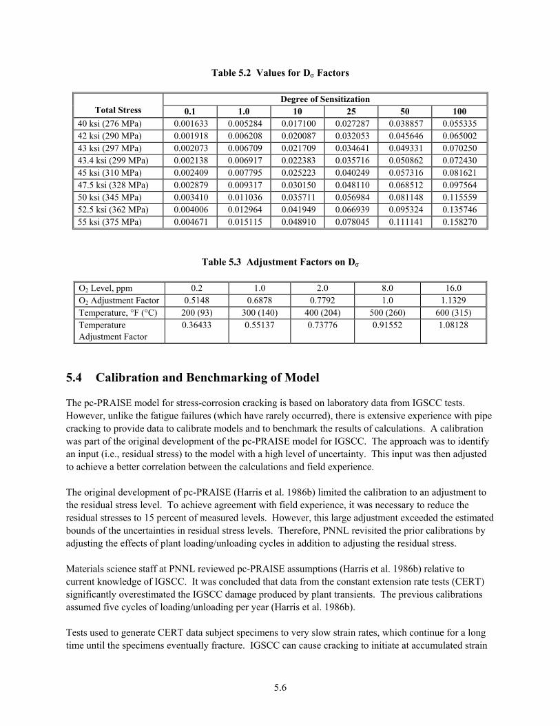
Table 5.2 Values for Dσ Factors
Degree of Sensitization Total Stress 0.1 1.0 10 25 50 100
40 ksi (276 MPa) 0.001633 0.005284 0.017100 0.027287 0.038857 0.055335 42 ksi (290 MPa) 0.001918 0.006208 0.020087 0.032053 0.045646 0.065002 43 ksi (297 MPa) 0.002073 0.006709 0.021709 0.034641 0.049331 0.070250 4 30 3.4 ksi (299 MPa) 0.002138 0.006917 0.022383 0.035716 0.050862 0.07244 0.040249 0.057316 0.081621 5 ksi (310 MPa) 0.002409 0.007795 0.025223 47.5 ksi (328 MPa) 0.002879 0.009317 0.030150 0.048110 0.068512 0.097564 50 ksi (345 MPa) 0.003410 0.011036 0.035711 0.056984 0.081148 0.115559 52.5 ksi (362 MPa) 0.004006 0.012964 0.041949 0.066939 0.095324 0.135746 55 ksi (375 MPa) 0.004671 0.015115 0.048910 0.078045 0.111141 0.158270
Table 5.3 Adjustment Factors on Dσ
O2 Level, ppm 0.2 1.0 2.0 8.0 16.0 O2 Adjustment Factor 0.5148 0.6878 0.7792 1.0 1.1329 Temperature, °F 600 (315) (°C) 200 (93) 300 (140) 400 (204) 500 (260) Temperature Adjustment Factor
0.36433 0.55137 0.73776 0.91552 1.08128
5.4 Calibration and Benchmarking o de
The pc-PRAISE model for rosion cracking ed o rator ta from IGSCC tests. However, unlike the fatigu ed), there is extensive experience with pipe racking to provide data to calibrate models and to benchmark the results of calculations. A calibration as part of the original development of the pc-PRAISE model for IGSCC. The approach was to identify
an input (i.e., residual stress) to the model with a high vel of uncertainty. This input was then adjusted achieve a better correlation between the calculations and field experience.
he original development of pc-PRAISE (Harris et al. 1986b) limited the calibration to an adjustment to
ted y
ssumptions (Harris et al. 1986b) relative to urrent knowledge of IGSCC. It was concluded that data from the constant extension rate tests (CERT)
damage produced by plant transients. The previous calibrations assumed five cycles of loading/unloading per year (Harris et al. 1986b).
time until the specimens eventually fracture. IGSCC can cause cracking to initiate at accumulated strain
f Mo l
stress-cor is bas n labo y dae failures (which have rarely occurr
cw
leto
Tthe residual stress level. To achieve agreement with field experience, it was necessary to reduce the residual stresses to 15 percent of measured levels. However, this large adjustment exceeded the estimabounds of the uncertainties in residual stress levels. Therefore, PNNL revisited the prior calibrations badjusting the effects of plant loading/unloading cycles in addition to adjusting the residual stress. Materials science staff at PNNL reviewed pc-PRAISE acsignificantly overestimated the IGSCC
Tests used to generate CERT data subject specimens to very slow strain rates, which continue for a long
5.6
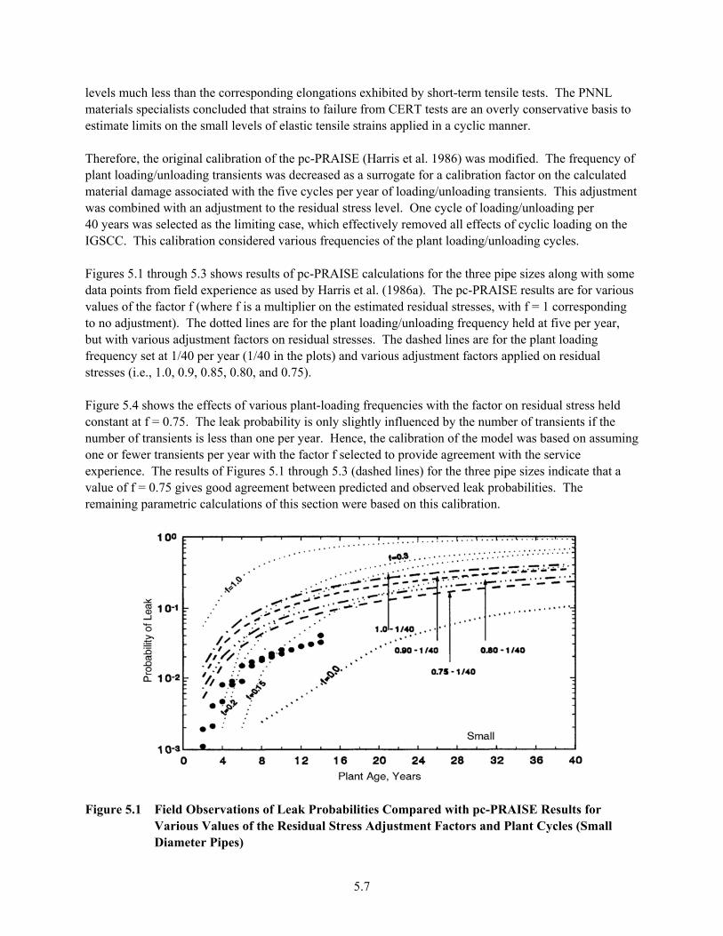
levels much less than the corresponding elongations exhibited by short-term tensile tests. The PNNL materials specialists concluded that strains to failure from CERT tests are an overly conservative basis to stimate limits on the small levels of elastic tensile strains applied in a cyclic manner.
herefore, the original calibration of the pc-PRAISE (Harris et al. 1986) was modified.lant loading/unloading transients was decreased as a surrogate for a calibration factor on the calculated
l d ading/unloading transients. This adjustment mb One cycle of loading/unloading per
n the
s
or the plant loading
y slightly influenced by the number of transients if the of the model was based on assuming
agreement with the service xperience. The results of Figures 5.1 through 5.3 (daalue of f = 0.75 gives good agreement between predicted and obs
e T The frequency of pmateria amage associated with the five cycles per year of lowas co ined with an adjustment to the residual stress level. 40 years was selected as the limiting case, which effectively removed all effects of cyclic loading oIGSCC. This calibration considered various frequencies of the plant loading/unloading cycles. Figures 5.1 through 5.3 shows results of pc-PRAISE calculations for the three pipe sizes along with somedata points from field experience as used by Harris et al. (1986a). The pc-PRAISE results are for variouvalues of the factor f (where f is a multiplier on the estimated residual stresses, with f = 1 corresponding to no adjustment). The dotted lines are for the plant loading/unloading frequency held at five per year,
ut with various adjustment factors on residual stresses. The dashed lines are fbfrequency set at 1/40 per year (1/40 in the plots) and various adjustment factors applied on residual stresses (i.e., 1.0, 0.9, 0.85, 0.80, and 0.75). Figure 5.4 shows the effects of various plant-loading frequencies with the factor on residual stress held onstant at f = 0.75. The leak probability is onlc
number of transients is less than one per year. Hence, the calibrationne or fewer transients per year with the factor f selected to provide o
e shed lines) for the three pipe sizes indicate that a erved leak probabilities. The v
remaining parametric calculations of this section were based on this calibration.
Figure 5.1 Field Observations of Leak Probabilities Compared with pc-PRAISE Results for
Various Values of the Residual Stress Adjustment Factors and Plant Cycles (Small Diameter Pipes)
5.7
Figure 5.2 Field Observations of Leak Probabilities Compared with pc-PRAISE Results for
Various Values of the Residual Stress Adjustment Factors and Plant Cycles (Intermediate Diameter Pipes)
Figure 5.3 Field Observations of Leak Probabilities Compared with pc-PRAISE Results for
Various Values of the Residual Stress Adjustment Factors and Plant Cycles (Large Diameter Pipes)
5.8
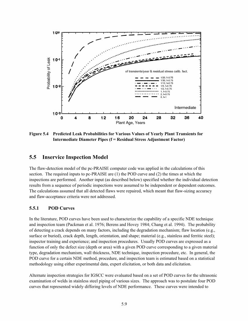
5.9
k Pr s for Va s for mediate Factor)
Inservice Inspection Model
calc of this ts to pc-PRAISE are (1) the POD curve and (2) the times at which the
ut (as described below) specified whether the individual detection m a sequence of periodic inspections were assum to be independent or dependent outcomes.
ons assu e flaw-sizing accuracy eptance criteri
y echnique . 1994). The probability
m; flaw location (e.g., itic steel);
ector train ecti d l ssed as a of on given POD curve corresponding to a given material
, wall thickness, NDE techni ection procedure, etc. In general, the method, p d inspection team
ental data, expert elicitation, or b icitation.
rnate es for IGSC ted based on a set of POD curves for the ultrasonic mination of welds in stainless steel piping ou four POD
curves that represented widely differing l performance.
Figure 5.4
5.5
The flaw-detection msection. The required inpuinspections are performresults froThe calculatiand flaw-acc 5.5.1
In the literature, POD curves have been used to and inspection teamof detecting a crack depends on msurface or buried), crack depth, length, inspfunction type, degradaPOD curve for a certain NDE methodolog Alteexa
Predicted LInter
ea Diamete
odel of the pc-PRAISE com
obabilr Pipes (f = Re
itie rious Values of Yearly Plant Transientsidual Stress
ter c
Adjustment
applied in tpu ode was he ulations
ed. Another inp
med that all detected flaws wa were not addressed.
man et al. 1976; Berens a
experien
ed
y
es.
re repaired, which meant that
nd Hoveng the degradad shape; material (e.g., stainless and ferr
oce
POD Curves
characterize the capabilit
on
of a specific NDE t
echanis (Pack
and
1984; Chang et al
U
an
; a
y factors, includi
nd i
tion m
ly POD curves are expreorientation, annsping ce pr ur sua
ly the defect size (depth or area) with a tion m
using either experim
ecti
echanism
on s
que, insp
s sizes. The approach was to postulate
rocedu
C wer
evels of
re, an
e evaluaof vari
NDE
is estimoth data and el
These curves were intended to
ated based on a statistical y
insp trategi
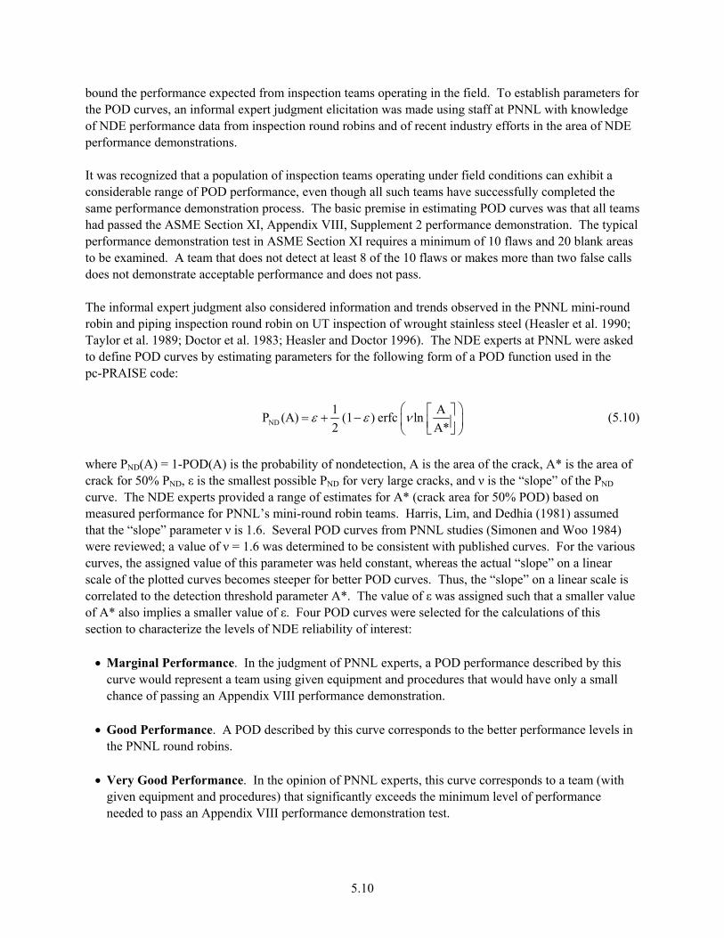
bound the performance expected from inspection teams operating in the field. To establish parameters for the POD curves, an informal expert judgment elicitation was made using staff at PNNL with knowledge
teams
pplement 2 performance demonstration. The typical erformance demonstration test in ASME Section XI requires a minimum of 10 flaws and 20 blank areas
e 10 flaws or makes more than two false calls does not demonstrate acceptable performance and does not pass.
-round
of NDE performance data from inspection round robins and of recent industry efforts in the area of NDE performance demonstrations. It was recognized that a population of inspection teams operating under field conditions can exhibit a considerable range of POD performance, even though all such teams have successfully completed thesame performance demonstration process. The basic premise in estimating POD curves was that all had passed the ASME Section XI, Appendix VIII, Supto be examined. A team that does not detect at least 8 of th
The informal expert judgment also considered information and trends observed in the PNNL minirobin and piping inspection round robin on UT inspection of wrought stainless steel (Heasler et al. 1990; Taylor et al. 1989; Doctor et al. 1983; Heasler and Doctor 1996). The NDE experts at PNNL were askedto define POD curves by estimating parameters for the following form of a POD function used in the pc-PRAISE code:
ND1 AP (A) (1 ) erfc ln2 A*
ε ε ν⎛ ⎞⎡ ⎤= + − ⎜ ⎟⎢ ⎥⎣ ⎦⎝ ⎠ (5.10)
PND , A* is the area of ND ND pe” of the PND
us
using given equipment and procedures that would have only a small chance of passing an Appendix VIII performance demonstration.
• Good Performance. A POD described by this curve corresponds to the better performance levels in
the PNNL round robins. • Very Good Performance. In the opinion of PNNL experts, this curve corresponds to a team (with
given equipment and procedures) that significantly exceeds the minimum level of performance needed to pass an Appendix VIII performance demonstration test.
where (A) = 1-POD(A) is the probability of nondetection, A is the area of the crackcrack for 50% P , ε is the smallest possible P for very large cracks, and ν is the “slocurve. The NDE experts provided a range of estimates for A* (crack area for 50% POD) based on measured performance for PNNL’s mini-round robin teams. Harris, Lim, and Dedhia (1981) assumed that the “slope” parameter ν is 1.6. Several POD curves from PNNL studies (Simonen and Woo 1984) were reviewed; a value of ν = 1.6 was determined to be consistent with published curves. For the variocurves, the assigned value of this parameter was held constant, whereas the actual “slope” on a linear scale of the plotted curves becomes steeper for better POD curves. Thus, the “slope” on a linear scale is correlated to the detection threshold parameter A*. The value of ε was assigned such that a smaller value of A* also implies a smaller value of ε. Four POD curves were selected for the calculations of this section to characterize the levels of NDE reliability of interest: • Marginal Performance. In the judgment of PNNL experts, a POD performance described by this
curve would represent a team
5.10
• Advanced Performance. This curve describes a level of performance significantly better than expected from present-day teams, equipment, and procedures that have passed an Appendix VIII-type of performance demonstration. This performance level implies advanced technologies and/or improved procedures that could be developed in the future.
Table 5.4 summarizes the input data for the above four POD curves, which are shown in Figure 5.5. These particular curves assume that POD is a function of the crack depth as a fraction of pipe-wall thickness, independent of the actual wall thickness. Parameters indicated in Table 5.4 are considered appropriate to wall thicknesses of 1.0 in. (2.54 cm) and greater. Lower levels of POD as a function of a/h should be assumed for thinner-walled pipe. The parameter a* is the crack depth for 50% probability of nondetection and is related to A* (i.e., A* = π/4 DB a*, where DB is the beam diameter of the ultrasonic probe).
Table 5.4 POD Curve Parameters for Four Performance Levels
Inspection Performance Level a*/t(a) ε ν
Marginal 0.65 0.25 1.4 Good 0.40 0.10 1.6 Very Good 0.15 0.02 1.6 Advanced 0.05 0.005 1.6 (a) t is the wall thickness of the pipe.
Figure 5.5 Probability of Detection Curves for Intergranular Stress-Corrosion Cracking
5.11
In this study, the value of a* is taken to vary linearly with wall thickness, t. This may or may not be the case in a given situation. The assigned value of ν is 1.4 for the marginal performance level and 1.6 for all the other performance levels. The ν values were obtained by examining the POD data for 10-in. (25.4-cm) stainless steel piping with stress-corrosion cracks generated by PNNL (Doctor et al. 1983; Simonen and Woo 1984). The smallest possible PND for a large crack is the largest for the marginal POD (i.e., 25%) and is the smallest for the advanced POD curve (i.e., 0.5%). 5.5.2 Factor of Improvement
The effectiveness of inservice inspection programs is quantified by a parameter called “factor of improvement” (Thomas 1979; Simonen 1990; Khaleel and Simonen 1994a, 1994b). In this section, the factor of improvement is based on the cumulative leak probabilities that occur over the 40-year design life of the plant, and the “factor of improvement” is defined as the ratio
leak probability at 40 years without NDEFactor of Improvement = leak probability at 40 years with NDE
(5.11)
.5.3 Independent versus Dependent Inspections
ection personnel, equipment, procedures, and other random ctors; and (2) systematic factors related to the flaw location, component geometry, etc. The four POD
urves presented earlier account for the degradation m and the variations due to the flaw metry, orientation, etc. In addressing the NDE reliability factors, which may change from
o tion that
he original version of pc-PRAISE (Harris and Dedhia 1992) addressed only the independent option for or the dependent assumption, PNNL echanics Technology to modify pc-PRAISE
5.12)
equal to the product of the probability of failure without inspection and the product of the values of the n
ast inspection). It is believed that field performance can
e bounded by the “dependent” and “independent” cases. Section 4 presents results that compare the
ith the being less sensitive to the assumption of dependent versus independent inspections.
5
Inspection unreliability comes mainly from two sources of variation: (1) factors that change from inspection, including inspinspection to
fac echanismlocation, geoinspection t inspection, the calculations of this section were based in most cases on the assumpthe series of inspections of a given weld over time are “dependent.” Tmodeling a sequence of inspections. To permit calculation fsubcontracted with Drs. Harris and Dedhia at Engineering Mto include the option of dependent inspections. When the probability of failure after n inspections is “independent” n
fP (t) ( isPOD curve evaluated at each previous inspection. If the inspections are “dependent,” credit is only takefor the last inspection (i.e., the probability of detecting the flaw over the course of all of the inspectionsequals the probability corresponding to only the lbresults of pc-PRAISE calculations for fatigue that compare the “dependent” case with results for the “independent” case. These results indicate significant differences when the inspection frequency is large (e.g., ISI at 1-year intervals). Sensitivity calculations for IGSCC have shown a similar trend, but wIGSCC results
5.12
5.5.4 Multiple Defects in a Given Weld
ion-
rack is
uction heating stress improvement (IHSI), were not addressed. The calculations focused
n leak probabilities because pc-PRAISE calculates probabilities of leaks more accurately and ica
med .
ase of the calculations included simulations of inservice inspections for a range of POD urves and inspection frequencies as indicated in Table 5.5. These calculations addressed only a selected
ver the full range of the Dσ parameter. Ratios of leak probabilities from the inspection simulation runs and the corresponding base-case runs
Welds are divided by pc-PRAISE into 2-in. (5.08-cm) segments. Each segment has only one corroscritical location where a crack can initiate. Cracks in neighboring segments may link to form larger cracks. The entire weld is assumed to be inspected at the time of each scheduled inspection. If a cdetected in the weld, the weld is repaired, and the entire weld regains its integrity (perfect repair.) 5.6 Input Parameters for Parametric Calculations
The parametric calculations concentrated on welds in 304 stainless steel piping and on the cumulative leak probabilities over a 40-year time frame of plant operation. Consideration of remedial actions for IGSCC was limited to inservice inspections. Other mitigative measures, such as hydrogen injection, weldoverlays, or indoeconom lly than probabilities of double-ended pipe breaks.
Table 5.5 summarizes the matrix of calculations along with the input parameters for the calculations. Base-case pc-PRAISE runs were first made for each of the three pipe sizes. These calculations assurealistic ranges for the various input variables that govern the initiation and growth of IGSCC cracksThe following variables were addressed: O2 content, temperature, coolant conductivity, applied stress, and frequency of heatup and cooldown (HUCD). The resulting calculations therefore covered the relevant range of the Dσ parameter used to present the results in a generalized manner. This initial set of pc-PRAISE runs assumed no inservice inspection and gave calculated 40-year cumulative leak probabilities ranging from 1.0E-04 to 1.0. The second phcsubset of the base-case calculations, but were sufficient to co
gave values for improvement factors. The establishment of these improvement factors for alternative inspection strategies was the primary objective of the calculations. 5.7 Results of Parametric Calculations
A large volume of numerical data was produced by completion of the parametric calculations for IGSCC of piping as described by Table 5.5. This section presents a collection of plots that show trends for pipe-leak probabilities and for the effectiveness of various inservice inspection strategies in reducing leak probabilities.
5.13

Table 5.5 Input Values f C
e
or Parametric Calculations for Piping Subject to IGSC
Pipe Siz
Including the Effects of Inservice Inspection
Input Parameter Small Medium Large Outside Diameter 46, in. (mm) 3. (88) 14.32 (364) 21.60 (549) Wall Thickness, i 34 ) n. (mm) 0. (8.6 0.84 (21.3) 1.04 (26.4) Welding Residuksi (MPa)
al an ze for a s
= 0.75 ress at ID
Mean = 24SD = 14.5
valuet of
valnt
Stress, Rsmf St
domill line
d pc-PRAISE input valueswith adjustment of
.40 (168) 8 (100)
Randomized pc-PRAISEmedium lines with adjusf = 0.75 Stress at ID Mean = 9.3 (64) SD = 14.47 (98)
input ment
s for Randomized pc-PRAISE inputfor medium lines with adjustmef = 0.75 Stress at ID Mean = 38.0 (262)
ues of
Axial ComponePrimary Stress,
nt of ksi (
to 15 (13.8 toMPa)
2 103) 2 to 15 (13.8 to 103) 2 to 12.5 (13.8 to 86)
Flow Stress of Material, ksi (M
Piping Pa)
ormal Distribean = 43.0 (2andard Devia 2 (
NMSt
ution 96) tion = 4.2 (29)
Normal Distribution Mean = 43.0 (296) Standard Deviation = 4. 29)
Normal Distribution Mean = 43.0 (296) Standard Deviation = 4.2 (29)
I tributi
ognormal Disteterministic Fl 25) ean Flaw Leape Paramet
0.2 2)
1)
nitial Flaw Disn. (mm)
ion, LDMSh
ribution aw Depth = 0.001 (0.0
ngth = 0.125 (3.2) er = 0.85
Lognormal Distribution Deterministic Flaw DeptMean Flaw Length = 0.1Shape Parameter = 0.85
h = 0.001 (5 (3.
025) Lognormal Distribution Deterministic Flaw Depth = 0.00Mean Flaw Length = 0.125 (3.2Shape Parameter = 0.85
(0.025)
Probability of DCurve
etecti ur POD Cur T 5.4 5.on Fo ves as per Table 5.4 Four POD Curves as per able Four POD Curves as per Table 4
Frequency of InYr) (Time of InSI/Frequency)
spect( itial I
10; 5/5; 2/2; ion, 5/ 1/1 5/10; 5/5; 2/2; 1/1 5/10; 5/5; 2/2; 1/1
Range of Dσ Paramet 39E-03 to 7.2er 2. 8E-03 2.94E-03 to 1.77E-02 1.07E-02 to 2.09E-02 and s per Eqs. (5. f Section 5. on 5.2 2 As per Eqs. (5.1)–(5.7) of SectiAs per Eqs. (5.1)–(5.7) o1)–(5.7) of Section 5.2A
5.14
Crack InitiationGrowth
5.7.1 Predicted Leak Probabilities versus Dσ
Figure 5.6 shows the cumulative leak probability at 40 years versus Dσ for large pipes. In the parametric calculations, many pc-PRAISE runs were performed to cover a range of leak probabilities from 1E-4 to 1.0. In these calculations for the large pipe size, the residual stress and degree of sensitization were kept constant (f = 0.75, Pa = 8). On the other hand, Figure 5.7 shows the 40-year cumulative leak probability versus Dσ for various degrees of sensitization, temperature, and oxygen content, but with the level of residual stress (f = 0.75) held constant. As shown by both figures, a strong correlation between the 40-year cumulative leak probabilities and Dσ exists. 5.7.2 Effect of Pipe Size on Leak Probabilities
Calculated leak probabilities are shown in Figure 5.8 for each of three pipe sizes for the assumption of no inservice inspection. For all pipe sizes, the leak probabilities increase as the Dσ value increases. However, each pipe size gives a separate trend curve. It is believed that different levels and distributions in welding residual stress for the various pipe sizes is a major contributing factor to the size dependence of the curves relating pipe leak probability to the Dσ parameter. It is seen that the two smaller pipe sizes have higher calculated leak probabilities than large pipe sizes. Figure 5.9 also shows the effect of pipe size on the calculated probabilities of a leak, but now as a function of time for a fixed value of Dσ (Dσ = 5.0E-03). Each curve shows a similar trend of increasing leak probability as a function of time with the large pipe size having the lowest probabilities and the intermediate pipe size having the highest probabilities. 5.7.3 Effect of POD Curve and ISI Frequency on Improvement Factor
The matrix of calculations addressed three pipe sizes (small, intermediate, and large), four POD curves (marginal, good, very good, and outstanding) and four inservice inspection intervals (10, 4, 2, and 1 year) giving 4 × 4 × 3 = 48 ISI scenarios. Detailed results of the calculated improvement factors associated with the inservice inspection cases are presented for reference purposes by Figures 5.10 through 5.30 below (see end of section for Figures 5.10 through 5.30). To maximize the usefulness of the plots, each set of results is presented both as a function of the Dσ parameter and of the corresponding leak probability (cumulative probability of through-wall crack at 40 years). The individual data points for improvement factors exhibited some data scatter, which was addressed by using a regression analysis to establish best-fit curves (second order polynomial) in terms of improvement factors versus the logarithm (base 10) of Dσ and the corresponding leak probabilities. For clarity, the plots below show only the best-fit curves rather than the individual data points.
5.15

Figure 5.6 Cumulative Leak Probability Over 40 Years as a Function of the Stress-Corrosion
mage Parameter; Dσ for Various Temperatures (°Da F) and Oxygen Contents (°C = [°F-32] / 1.8)
Figure 5.7 The Effect of Various Degrees of Sensitization on the Relationship Between the
40-Year Cumulative Leak Probability and Dσ (°C = [°F-32] / 1.8)
5.16
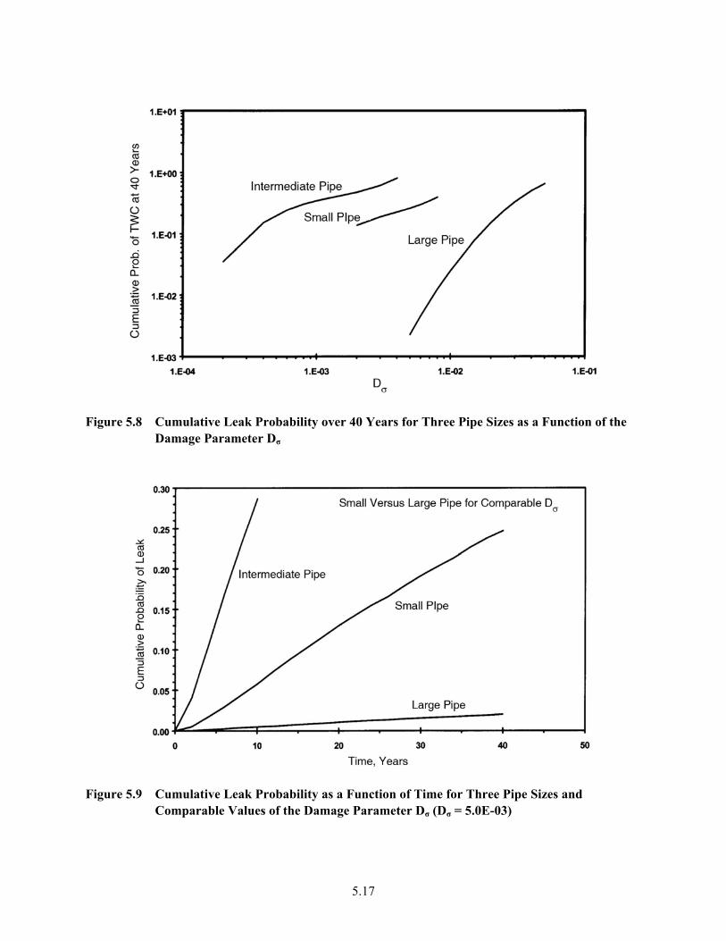
Figure 5.8 Cumulative Leak Probability over 40 Years for Three Pipe Sizes as a Function of the
r D Damage Paramete σ
Figure 5.9 Cumulative Leak Probability as a Function of Time for Three Pipe Sizes and
Comparable Values of the Damage Parameter Dσ (Dσ = 5.0E-03)
5.17
5.7.4 Improvement Factors for Small Pipe Size
Figures 5.10 through 5.17 show predicted improvements in reliability over a 40-year design life for the small pipe size that results from inservice inspections performed over the 40-year operating period. Four different levels of NDE performance are addressed. In Figures 5.10 through 5.13, the inspection method (POD curve) was held constant, and the inspection intervals ranged from 1 to 10 years. Figures 5.14 through 5.17 show the same set of results, but with the curves rearranged to maintain a common inspection interval for each plot, with the individual curves corresponding to different POD curves. Figure 5.10 (and successive figures) describes inspections performed at a 10-year interval and with the first inspection at the 10th year using the notation 10/10. Similarly, 4/4 indicates inspections at 4-year intervals with the first inspection at the 4th year. It is seen that POD curves with the better detection probabilities always increase the factor improvement, no matter what inspection interval is used. However, the results for the small pipe size show that even the “outstanding” POD curve requires frequent inspection to achieve meaningful reductions in failure probabilities.
rom Figure 5.10, it is seen that the “marginal” POD curve provides little benefit in reducing the a
inspections with 11 and 5.12) give more meaningful nhancement in piping reliability. The greatest benefits are predicted for the “outstanding” NDE chnology and procedures, for which an order-of-magnitude improvement on the leak probability can be
achieved for an inspection frequency of once per year. This improvement factor of 10 is still significantly ss than the theoretical limit of 200 (1/ε = 1/0.005 = 200) for the “outstanding” POD curve. In contrast,
factors of about t a frequency of once er year. The lower benefits of ISI for IGSCC compared to the benefits for fatigue crack growth can be xplained in terms of long incubation periods for stress-corrosion cracking followed by a period of rapid
crack growth. 5.7.5 Improvement Factors for Intermediate Pipe Size
Figures 5.18 through 5.25 show the calculated improvement factors in the reliability (over a 40-year design life) for the intermediate pipe size. The simulated inservice inspections performed over the 40-year operating period were the same as those for the small pipe size. In the case of Figures 5.18 through 5.21, the inspection method (POD curve) was held constant for each figure, and the time intervals between inspections were varied from 1 to 10 years. Figures 5.22 through 5.25 show the same set of results, but with the curves rearranged to maintain a common inspection interval for each plot, with the individual curves corresponding to different POD capabilities. As for the small pipe size, the POD curves with the better detection probabilities always produce greater improvement factors. Nevertheless, even the “outstanding” POD curve requires frequent inspections to achieve meaningful reductions in failure probabilities.
Fprobability of f ilure, even when the inspection interval is reduced to one inspection per year. The
the “good” and “very good” POD curves (Figures 5.ete
lecomparable results given in Section 4 on fatigue crack growth indicate more encouraging improvement
100 for inspections using the “outstanding” POD curve performed ape
5.18

5.7.6 Improvement Factors for Large Pipe Size
Figures 5.26 through 5.30 show calculated improvement factors (over a 40-year design life) for the large pipe size. The number of simulated inservice inspection scenarios was somewhat more limited than for the small and intermediate pipe sizes. Figures 5.26 through 5.28 each address a specific inspection method (POD curve) with the individual curves corresponding to different inspection intervals ranging from 1 to 10 years. Figures 5.29 and 5.30 have rearranged the curves to maintain a common inspection interval for each plot, with the individual curves corresponding to different POD capabilities. As for the smaller pipe sizes, the POD curves with the better detection probabilities give greater improvement factors. In general, it appears that a given inspection strategy (combination of POD curve and inspection interval) gives somewhat greater improvement factors for the large pipe than predicted for the smaller sizes of pipe. 5.7.7 Effect of Pipe Size on Improvement Factor
Differences in calculated improvement factors for the three pipe sizes are indicated in Figures 5.31 through 5.35. As indicated by Figure 5.31, a better alignment of the improvement factor curves results when the data are plotted against leak probability (Figure 5.31b) rather than against Dσ (Figure 5.31a).
or this reason, the remaining plots (Figures 5.33 through 5.35) for several combinations of POD curves
he differences in the calculated improvement factors for the three pipe sizes are believed to be mainly ue to the different through-wall distributions of the welding residual stresses than to an effect of pipe
size per se. There is a consistent trend that shows greater benefits from inspections for the large pipe as ompared to the small or intermediate pipe size. This can be explained in terms of differences in the
s p
cations relative ated in the rge pipe would exhibit relatively uniform growth rates, making such cracks easier to detect by periodic
inations. In contrast, initiated cracks in the smaller pipes are believed to grow very slowly for extended time periods, followed by a short period of rapidly accelerated crack growth until a leak results. Detection of such a rapidly growing crack would require relatively small time intervals between the periodic inspections. 5.7.8 Time Dependence of Calculated Failure Probabilities
A final set of plots (Figures 5.36 and 5.37) show leak probability as a function of time, in contrast to all previous plots that only indicate the cumulative leak probability at the single time of 40 years. Figure 5.36 shows how the calculated leak probabilities for the three pipe sizes increase with time. It also shows that the failure rate (slope of the curves) remains relatively constant of the 40-year time span covered by the plots. In one case (Figure 5.36a), the Dσ for each pipe size was selected to give a leak probability at 40 years of about 20 percent. In the other case (Figure 5.36b), a common value of Dσ is equal to about 5.0E-03, which results in a large difference in the calculated leak probabilities for the three pipe sizes.
Fand inspection intervals have used leak probability as the independent variable.
Td
cthrough-wall distributions of residual stresses. The default stress distribution for the large pipe showrelatively stee stress gradients near the inner surface of the pipe and becomes compressive at subsurface
ly close to the inner surface. It would therefore be expected that cracks initilolaexam
5.19
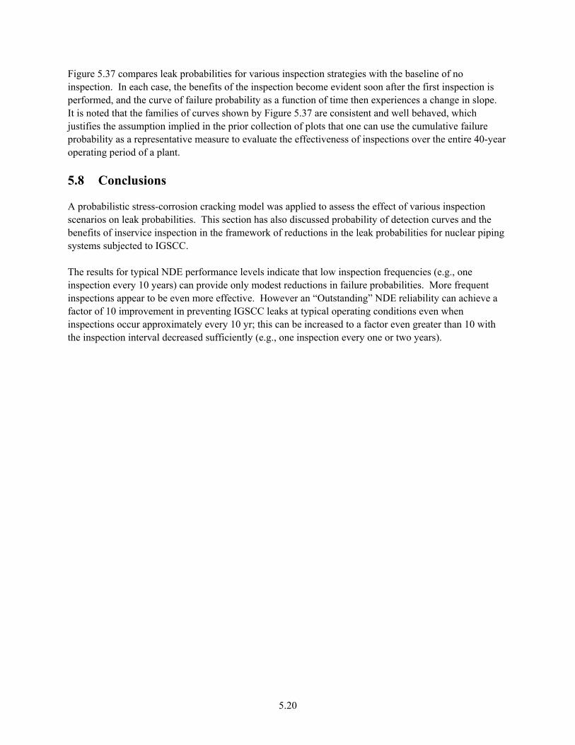
Figure 5.37 compares leak probabilities for various inspection strategies with the baseline of no inspection. In each case, the benefits of the inspection become evident soon after the first inspection is performed, and the curve of failure probability as a function of time then experiences a change in slope. It is noted that the families of curves shown by Figure 5.37 are consistent and well behaved, which justifies the assumption implied in the prior collection of plots that one can use the cumulative failure probability as a representative measure to evaluate the effectiveness of inspections over the entire 40-year operating period of a plant. 5.8 Conclusions
A probabilistic stress-corrosion cracking model was applied to assess the effect of various inspection scenarios on leak probabilities. This section has also discussed probability of detection curves and the benefits of inservice inspection in the framework of reductions in the leak probabilities for nuclear piping systems subjected to IGSCC. The results for typical NDE performance levels indicate that low inspection frequencies (e.g., one inspection every 10 years) can provide only modest reductions in failure probabilities. More frequent inspections appear to be even more effective. However an “Outstanding” NDE reliability can achieve a
ctor of 10 improvement in preventing IGSCC leaks at typical operating conditions even when ith
the inspection in tion every one or two years).
fainspections occur approximately every 10 yr; this can be increased to a factor even greater than 10 w
terval decreased sufficiently (e.g., one inspec
5.20
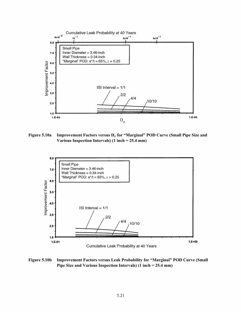
Figure 5.10a Improvement Factors versus Dσ for “Marginal” POD Curve (Small Pipe Size
Various Inspection Intervals) (1 inch = 25.4 mm) and
Figure 5.10b Improvement Factors versus Leak Probability for “Marginal” POD Curve (Small
Pipe Size and Various Inspection Intervals) (1 inch = 25.4 mm)
5.21
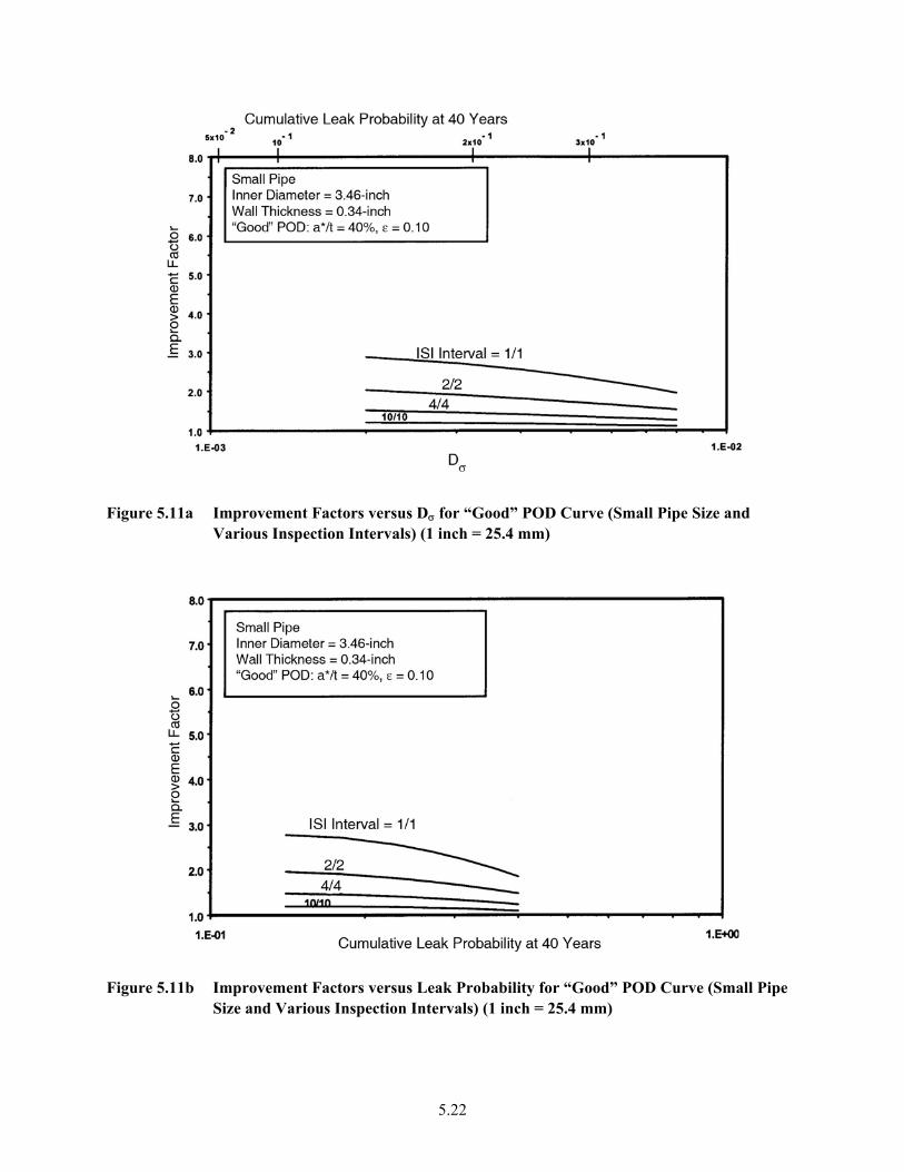
Figure 5.11a Improvement Factors versus Dσ for “Good” POD Curve (Small Pipe Size and
Various Inspection Intervals) (1 inch = 25.4
mm)
Figure 5.11b Improvement Factors versus Leak Probability for “Good” POD Curve (Small Pipe
Size and Various Inspection Intervals) (1 inch = 25.4 mm)
5.22
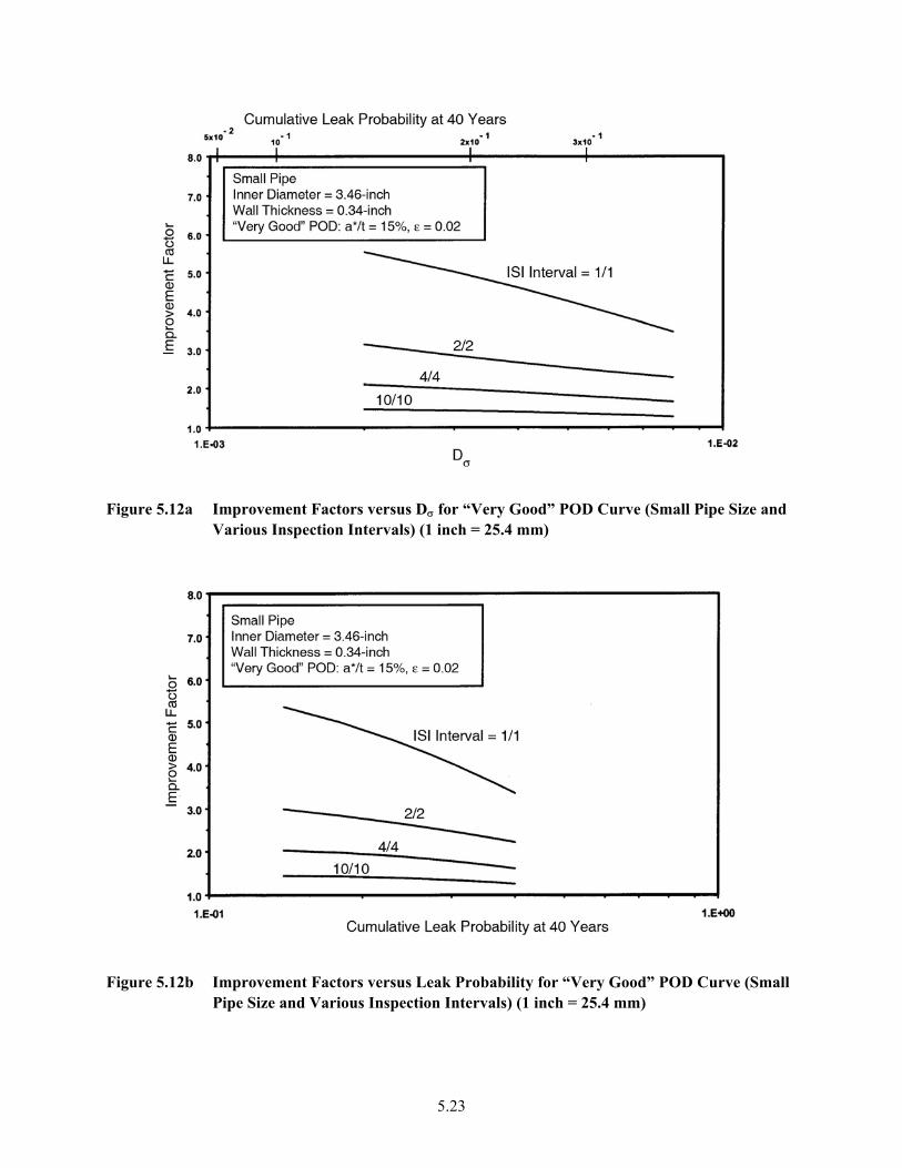
Figure 5.12a Improvement Factors versus Dσ for “Very Good” POD Curve (Small Pipe Siz
Various Inspection Intervals) (1 inch = 25.4e and
mm)
Figure 5.12b Improvement Factors versus Leak Probability for “Very Good” POD Curve (Small
Pipe Size and Various Inspection Intervals) (1 inch = 25.4 mm)
5.23
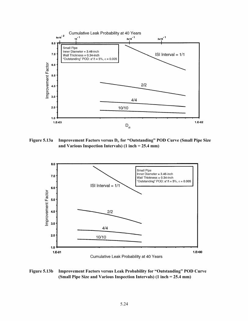
Figure 5.13a Improvement Factors versus Dσ for “Outstanding” POD Curve (Small Pipe Size
and Various Inspection Intervals) (1 inch = 25.4 mm)
Figure 5.13b Improvement Factors versus Leak Probability for “Outstanding” POD Curve
(Small Pipe Size and Various Inspection Intervals) (1 inch = 25.4 mm)
5.24
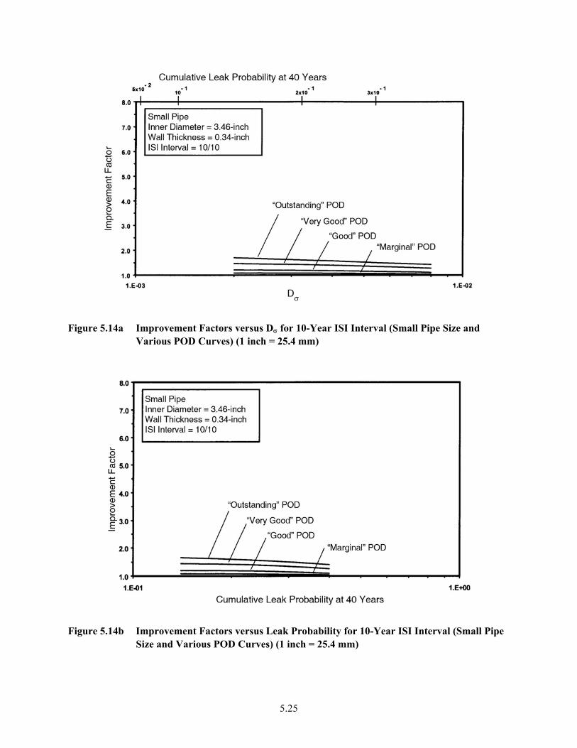
Figure 5.14a Improvement Factors versus Dσ for 10-Year ISI Interval (Small Pipe Size and
Various POD Curves) (1 inch = 25.4 mm)
Figure 5.14b Improvement Factors versus Leak Probability for 10-Year ISI Interval (Small Pipe
Size and Various POD Curves) (1 inch = 25.4 mm)
5.25
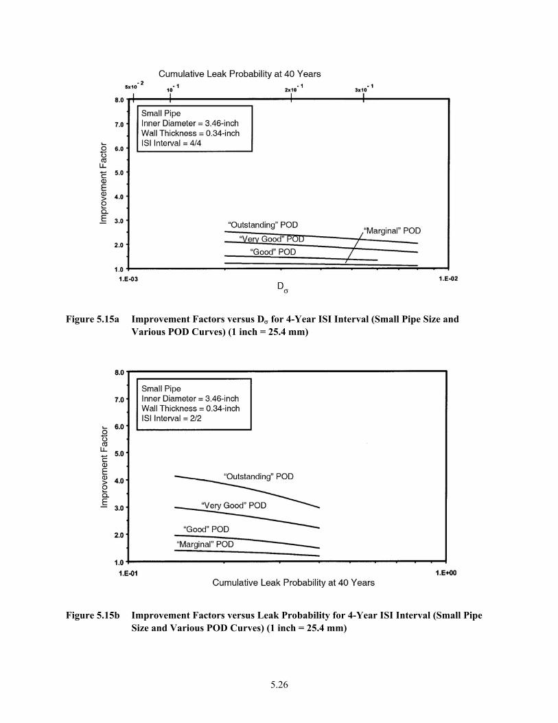
Figure 5.15a Improvement Factors versus Dσ for 4-Year ISI Interval (Small Pipe Size and
Various POD Curves) (1 inch = 25.4 mm)
Figure 5.15b Improvement Factors versus Leak Probability for 4-Year ISI Interval (Small Pipe
Size and Various POD Curves) (1 inch = 25.4 mm)
5.26
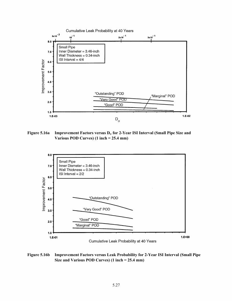
Figure 5.16a Improvement Factors versus Dσ for 2-Year ISI Interval (Small Pipe Size and
Various POD Curves) (1 inch = 25.4 mm)
Figure 5.16b Improvement Factors versus Leak Probability for 2-Year ISI Interval (Small Pipe
Size and Various POD Curves) (1 inch = 25.4 mm)
5.27
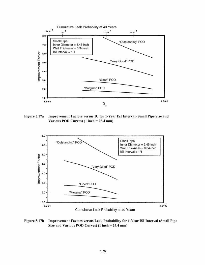
Figure 5.17a Improvement Factors versus Dσ for 1-Year ISI Interval (Small Pipe Size and
Various POD Curves) (1 inch = 25.4 mm)
Figure 5.17b Improvement Factors versus Leak Probability for 1-Year ISI Interval (Small Pipe
Size and Various POD Curves) (1 inch = 25.4 mm)
5.28
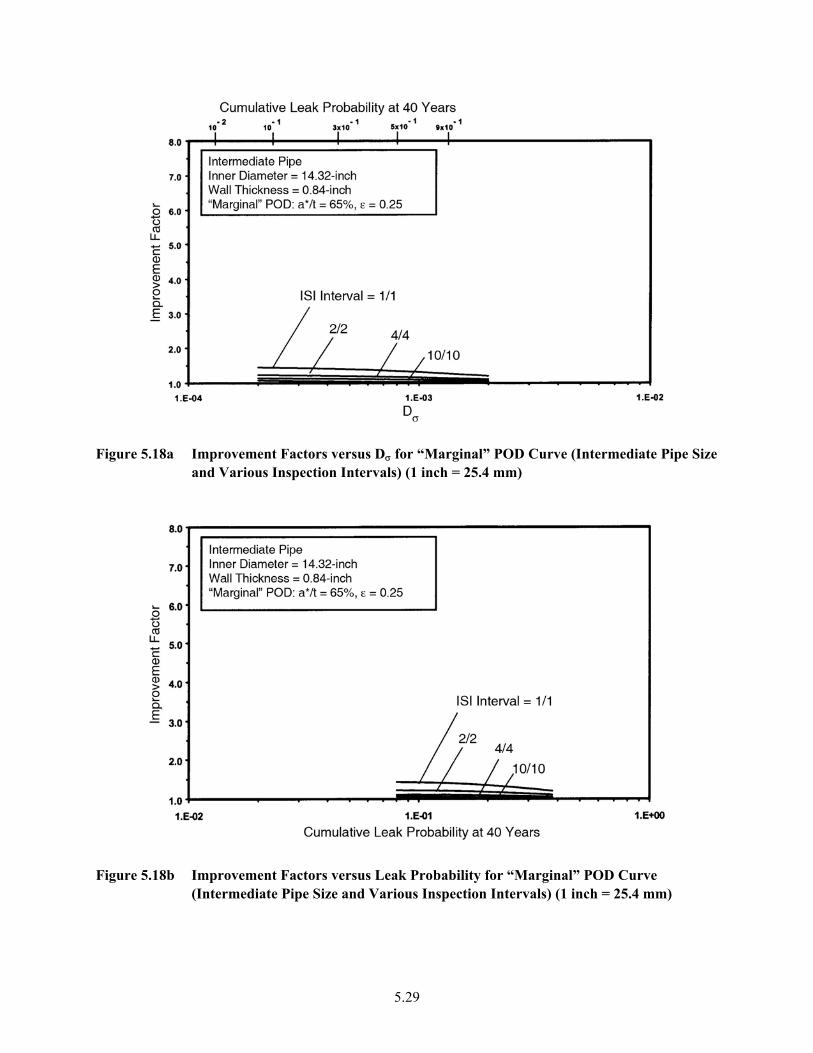
Figure 5.18a Improvement Factors versus Dσ for “Marginal” POD Curve (Intermediate Pipe Size
and Various Inspection Intervals) (1 inch = 25.4 mm)
Figure 5.18b Improvement Factors versus Leak Probability for “Marginal” POD Curve
(Intermediate Pipe Size and Various Inspection Intervals) (1 inch = 25.4 mm)
5.29
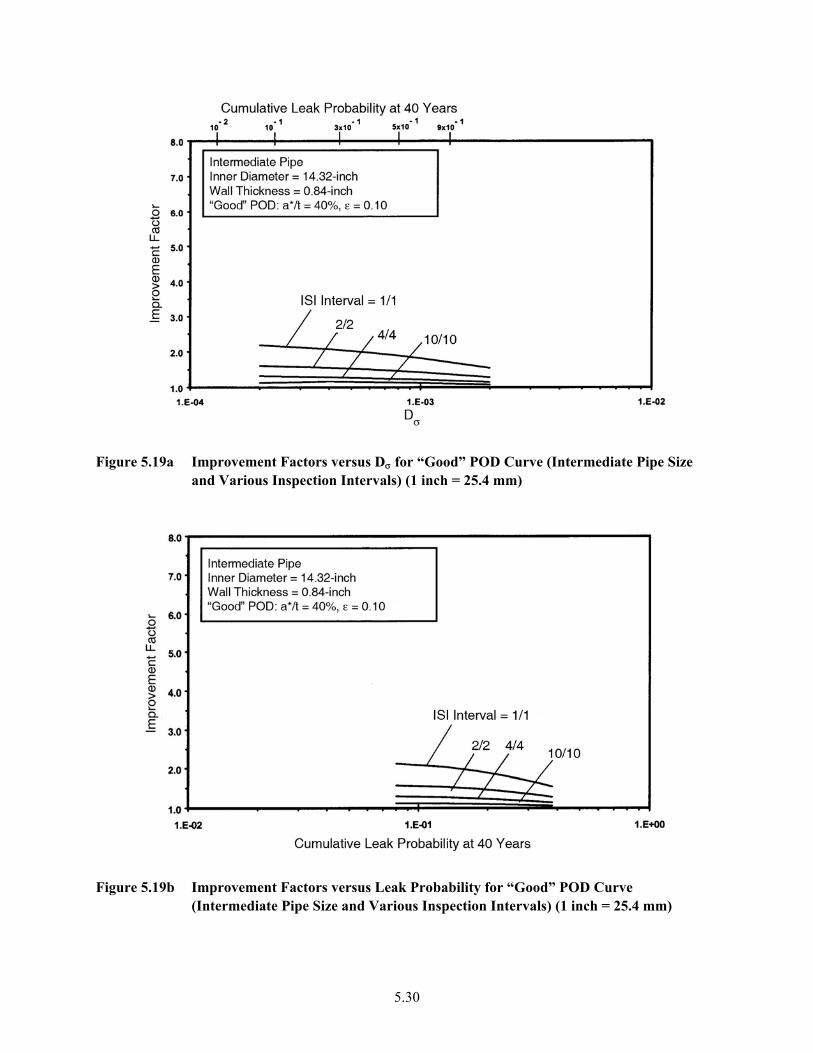
Figure 5.19a Improvement Factors versus Dσ for “Good” POD Curve (Intermediate Pipe Size
and Various Inspection Intervals) (1 inch = 25.4 mm)
Figure 5.19b Improvement Factors versus Leak Probability for “Good” POD Curve
(Intermediate Pipe Size and Various Inspection Intervals) (1 inch = 25.4 mm)
5.30

Figure 5.20a Improvement Factors versus Dσ for “Very Good” POD Curve (Intermediate Pipe
Size and Various Inspection Intervals) (1 inch = 25.4 mm)
Figure 5.20b Improvement Factors versus Leak Probability for “Very Good” POD Curve
(Intermediate Pipe Size and Various Inspection Intervals) (1 inch = 25.4 mm)
5.31
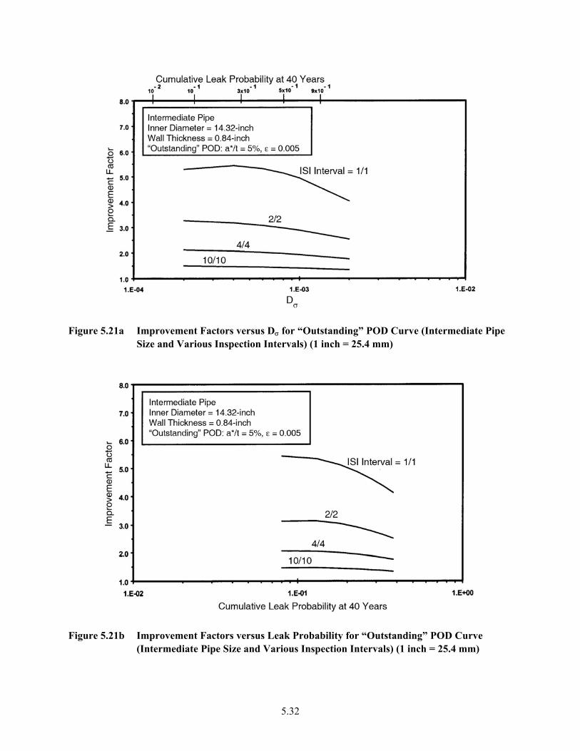
Figure 5.21a Improvement Factors versus Dσ for “Outstanding” POD Curve (Intermediate Pipe
Size and Various Inspection Intervals) (1 inch = 25.4 mm)
Figure 5.21b Improvement Factors versus Leak Probability for “Outstanding” POD Curve
(Intermediate Pipe Size and Various Inspection Intervals) (1 inch = 25.4 mm)
5.32
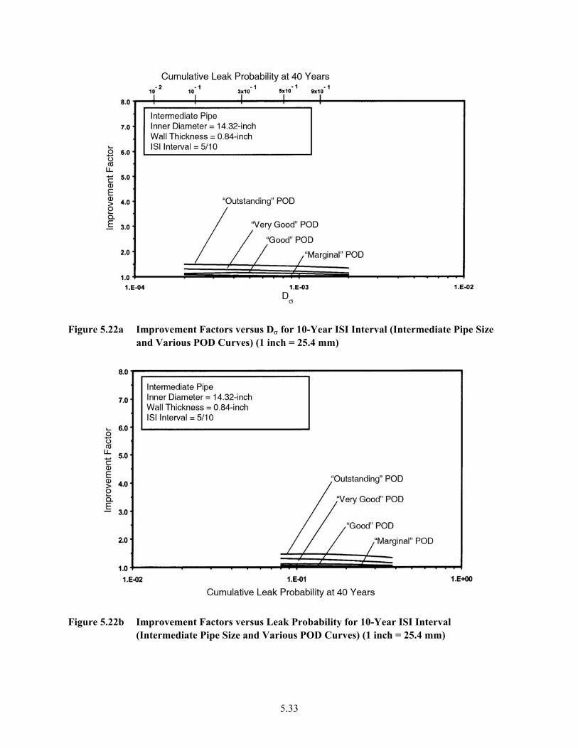
Figure 5.22a Improvement Factors versus Dσ for 10-Year ISI Interval (Intermediate Pipe Siz
and Various POD Curves) (1 inch = 25.4 me
m)
Figure 5.22b Improvement Factors versus Leak Probability for 10-Year ISI Interval
(Intermediate Pipe Size and Various POD Curves) (1 inch = 25.4 mm)
5.33
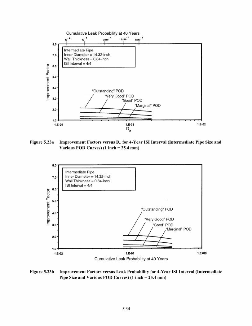
Figure 5.23a Improvement Factors versus Dσ for 4-Year ISI Interval (Intermediate Pipe Siz
Various POD Curves) (1 inch = 25.4 mm) e and
Figure 5.23b Improvement Factors versus Leak Probability for 4-Year ISI Interval (Intermediate
Pipe Size and Various POD Curves) (1 inch = 25.4 mm)
5.34
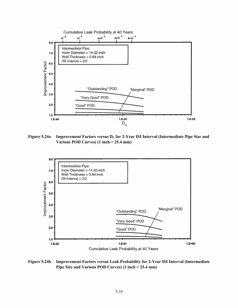
Figure 5.24a Improvement Factors versus Dσ for 2-Year ISI Interval (Intermediate Pipe Size and
Various POD Curves) (1 inch = 25.4 mm)
Figure 5.24b Improvement Factors versus Leak Probability for 2-Year ISI Interval (Intermediate
Pipe Size and Various POD Curves) (1 inch = 25.4 mm)
5.35
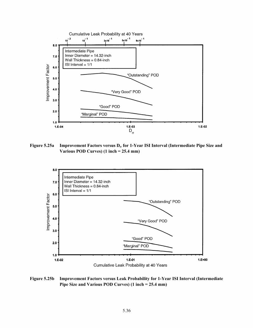
Improvement Factors versus Dσ forFigure 5.25a 1-Year ISI Interval (Intermediate Pipe Size and Various POD Curves) (1 inch = 25.4 mm)
Figure 5.25b Improvement Factors versus Leak Probability for 1-Year ISI Interval (Intermediate
Pipe Size and Various POD Curves) (1 inch = 25.4 mm)
5.36
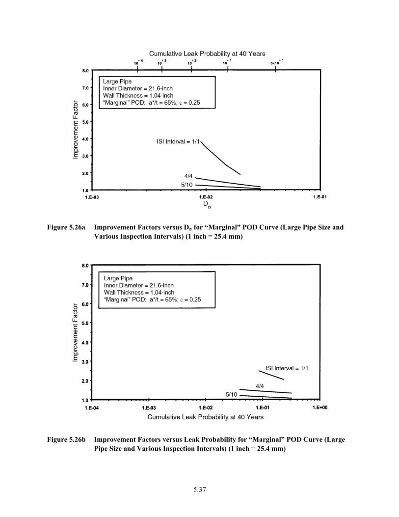
Figure 5.26a Improvement Factors versus Dσ for “Marginal” POD Curve (Large Pipe Size and
Various Inspection Intervals) (1 inch = 25.4 mm)
Figure 5.26b Improvement Factors versus Leak Probability for “Marginal” POD Curve (Large
Pipe Size and Various Inspection Intervals) (1 inch = 25.4 mm)
5.37
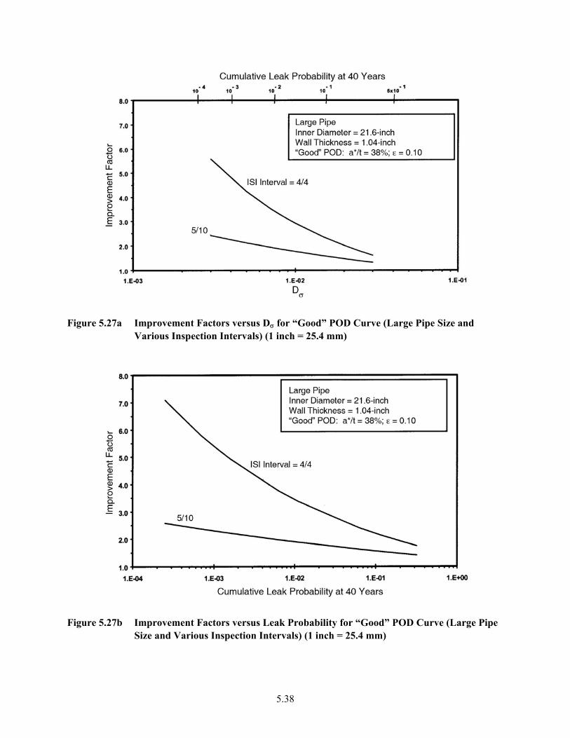
Figure 5.27a Improvement Factors versus Dσ for “Good” POD Curve (Large Pipe Size and
Various Inspection Intervals) (1 inch = 25.4 mm)
Figure 5.27b Improvement Factors versus Leak Probability for “Good” POD Curve (Large Pipe
Size and Various Inspection Intervals) (1 inch = 25.4 mm)
5.38
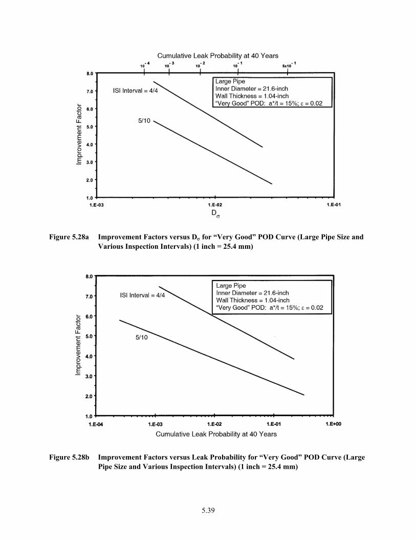
Improvement Factors versus Dσ forFigure 5.28a “Very Good” POD Curve (Large Pipe Size and Various Inspection Intervals) (1 inch = 25.4 mm)
Figure 5.28b Improvement Factors versus Leak Probability for “Very Good” POD Curve (Large
Pipe Size and Various Inspection Intervals) (1 inch = 25.4 mm)
5.39
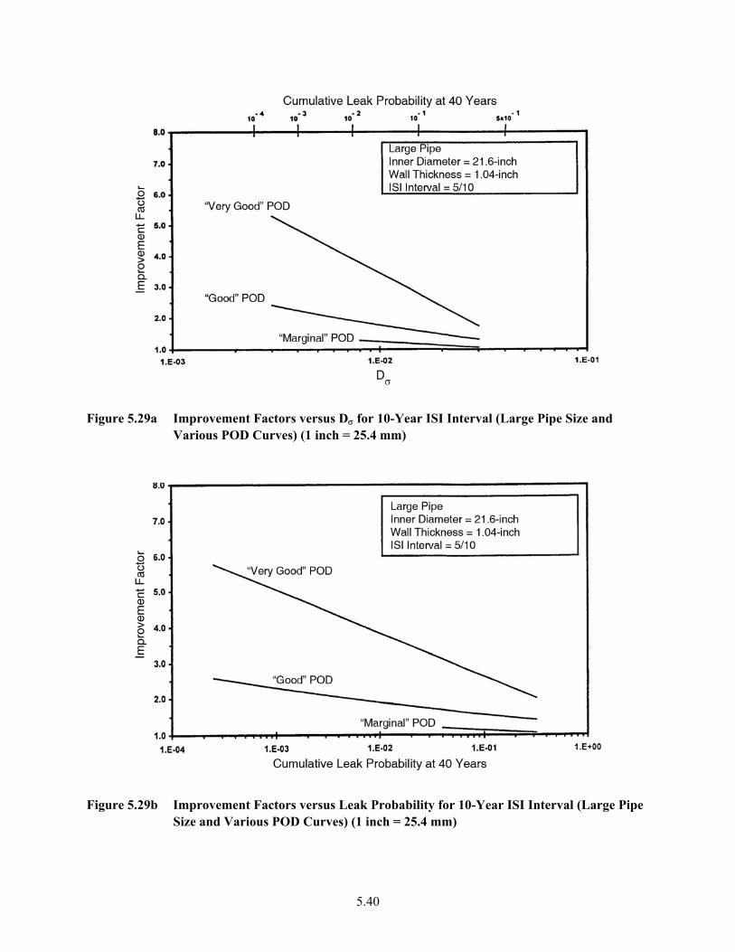
Figure 5.29a Improvement Factors versus Dσ for 10-Year ISI Interval (Large Pipe Size and
Various POD Curves) (1 inch = 25.4 mm)
ure 5.29b Improvement Factors versus Leak Probability for 10-Year ISI Interval (LargeSize and
Fig Pipe
Various POD Curves) (1 inch = 25.4 mm)
5.40

Figure 5.30a Improvement Factors versus Dσ for 4-Year ISI Interval (Large Pipe Size and
Various POD Curves) (1 inch = 25.4 mm)
Figure 5.30b Improvement Fac ersus Lea obability Year ISI rval (Lar pe
Size and Various POD Curves) (1 inch = 25.4 mm)
tors v k Pr for 4- Inte ge Pi
5.41
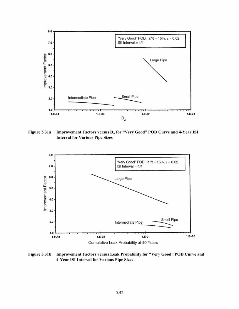
Fig
ure 5 Im vement Factors versus Dσ for “Very Good” PODa V ou S
.31a proterv
Curve and 4-Year ISI In l for ari s Pipe izes
Figure 5 Improvemen ct ve ea robabil or er Curve and
r
.31b 4-
t Faterval
ors rsu for Var
s Lious P
k Pipe S
ity f “V y Good” POD Yea ISI In izes
5.42
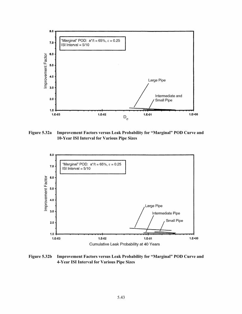
Figure 5.32a Improvement Factors versus Leak Probability for “Marginal” POD Curve and
10-Year ISI Interval for Various Pipe Sizes
Figure 5.32b Improvement Factors versus Leak Probability for “Marginal” POD Curve and
4-Year ISI Interval for Various Pipe Sizes
5.43
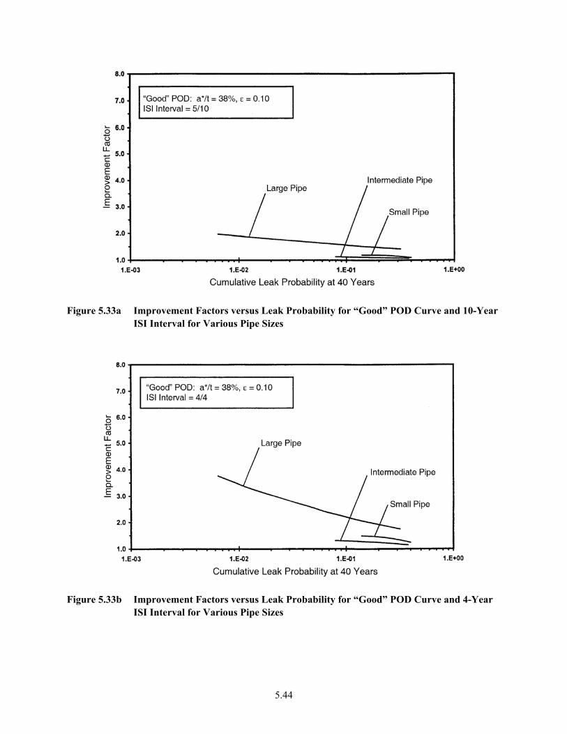
5.44
Figur 33a rs k Pro
erval for Various Pipe Sizes
e 5. Improvement Facto versus Lea bability for “Good” POD Curve and 10-Year ISI Int
Figur 33b rs k Pro ” POD rve and 4 ear
erval for Various Pipe Sizes e 5. Improvement Facto versus Lea bability for “Good Cu -Y
ISI Int
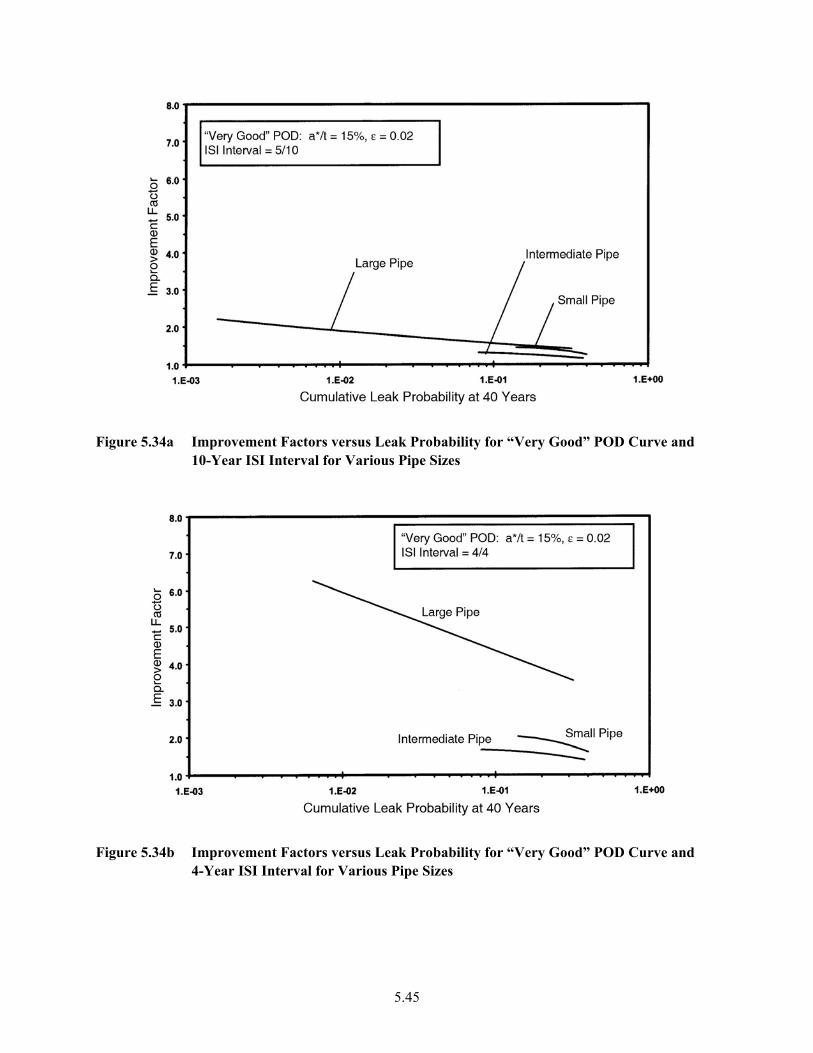
Figure 5.34a Improvement Factors versus Leak Probability for “Very Good” POD Curve and
10-Year ISI Interval for Various Pipe Sizes
Figure 5 us Leak P ery Good” POD Curve and
arious Pipe
.34b Improvement Factors vers robability for “VSizes 4-Year ISI Interval for V
5.45
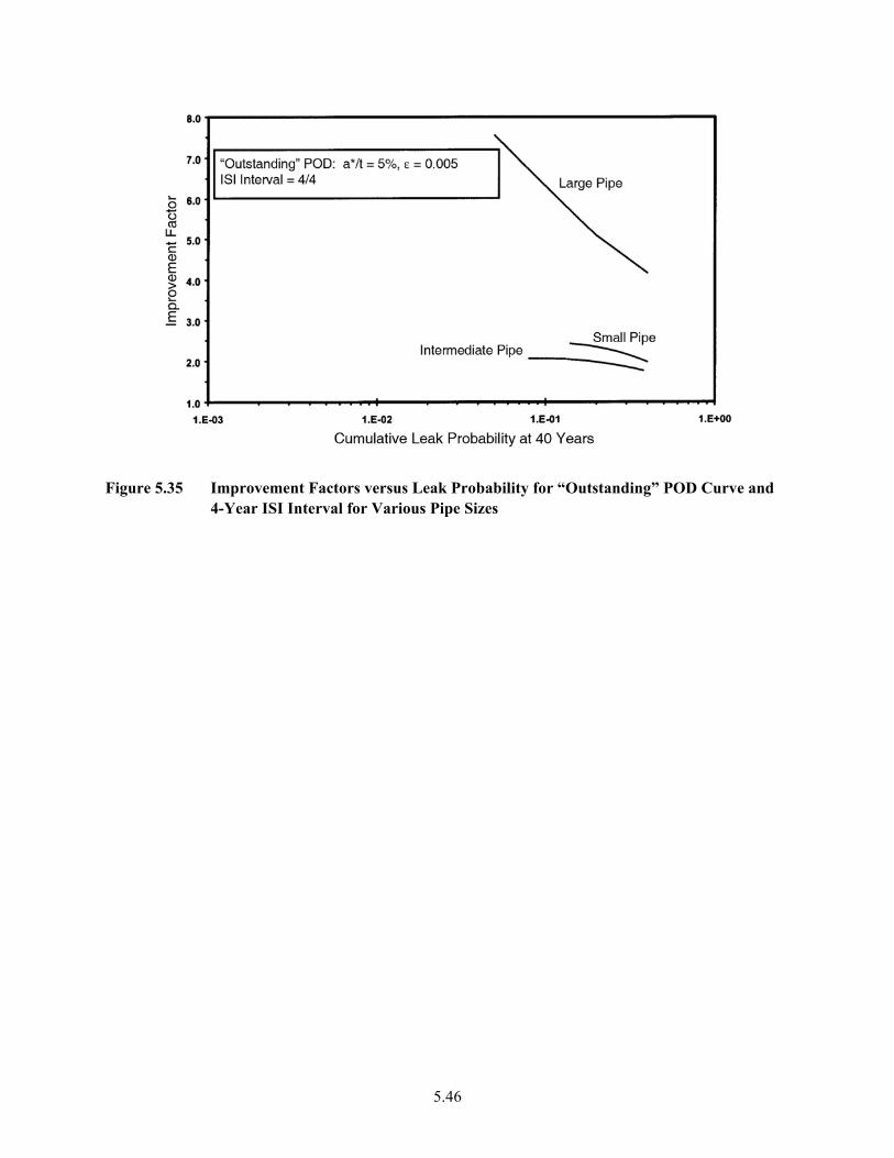
Figure 5.35 Improvement Factors versus Leak Probability for “Outstanding” POD Curve and
4-Year ISI Interval for Various Pipe Sizes
5.46
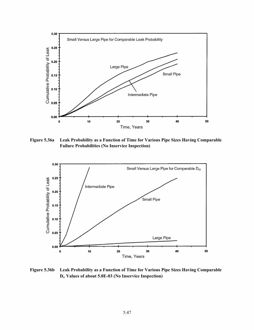
Figure 5.36a Leak Probability as a Function of Time for Various Pipe Sizes Having Comparable
Failure Probabilities (No Inservice Inspection)
Figure 5.36b Leak Probability as a Function of Time for Various Pipe Sizes Having Comparable
Dσ Values of about 5.0E-03 (No Inservice Inspection)
5.47
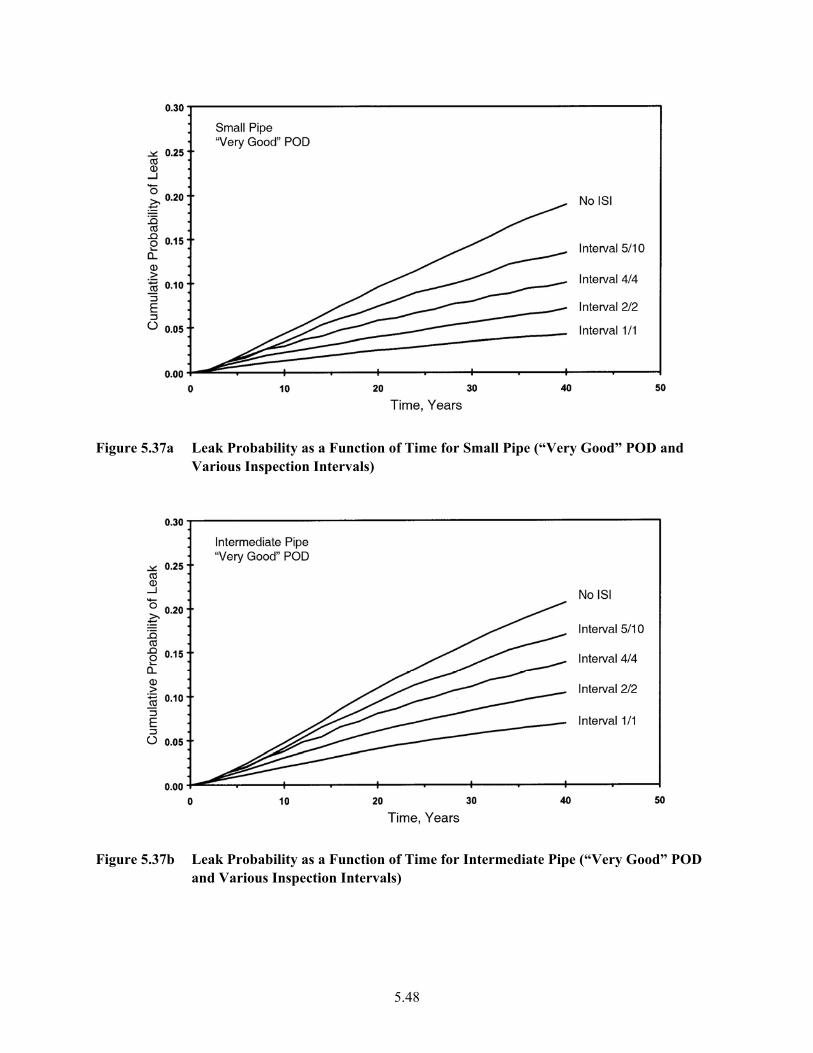
a Leak ProbabilitFigure 5.37 y as a Function of Time for Small Pipe (“Very Good” POD and Various Inspection Intervals)
Figure 5.37b Leak Probability as a Function of Time for Intermediate Pipe (“Very Good” PO
and Various Inspection Intervals)
D
5.48
6 Uncertainty Analysis for Calculated Failure Probabilities of Piping Welds
Introduction
ressure-bou ponents such as pressure vessels (Dickson 1994) and welds in piping systems arris et al. 1981; Harris and Dedhia 1992). The objective of the work described in this section was to
uantify the uncertainties associated with the inputs to PFM calculations and the uncertainties in the PFM model itself, as well as the uncertainties in the resulting calculated piping-failure probabilities. Such uncertainties are an important issue in applying PFM models (Bishop 1997) to the implementation of risk-informed procedures for developing improved inservice inspection programs (ASME/CRTD 1992; Westinghouse Owners Group 1997). The work presented here was an important part of the research that was intended to develop improved methods for predicting the reliability of nuclear piping systems and the effect of inservice inspections on reducing piping-failure probabilities. All calculations presented below used the pc-PRAISE computer code (Harris and Dedhia 1992) to address both leak and break probabilities for piping components. A two-step process was used to quantify the uncertainties in calculated failure probabilities (Simonen and Khaleel 1998b). The first step was a sensitivity study that identified those uncertainties having the greatest effect on the results from pc-PRAISE. The second step was a quantitative uncertainty analysis that addressed the most critical parameters as identified by the sensitivity calculations. While the selected methodology is generally applicable to PFM calculations for piping, the calculations described within this section address specific examples as follows:
• A single pipe thickness of 0.5
• A wide range of cyclic stresses are addressed using t r approach of Khaleel a n
(1994a,b) with Q factors of 1, 100, and 10 The ue corresponds to typical locations in piping systems for which fatigue failures are not exp reas th alue to locations exposed to thermal fatigue by which the pi nces u nd ex els of cyclic stress.
• While probabilities of both leak (through-wall crack reak ated,
interest was in the uncertainties for leak probabilities. Uncertainties in leak probabilities were of particular interest to the development of a Regulatory Guide on Risk-Informed Inservice Inspection
6.1
Probabilistic structural mechanics models are increasingly being used to predict the reliability of nuclear ndary comp
(Hq
• Mechanical and thermal fatigue of stainless steel piping due to the presence of fabrication defects (the
initiation of fatigue cracks is not addressed).
size (6-in. [152-mm] Schedule 120) with an inner radius of 2.75-in. (70 mm) and a wall 62 in. (14.3 mm).
he Q-facto nd Simone,000. lowest val
ected, whe e highest v correspondspe experie nexpected a cessive lev
) and pipe b were calcul the main
(Parry 1997) and to the application of the “Perdue Model” for weld inspection sampling plans (Balkey et al. 1997).
6.1
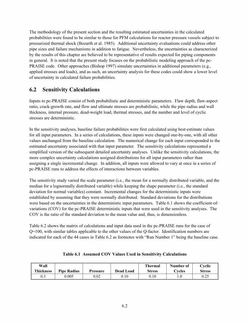
The methodology of the present section and the resulting estimated uncertainties in the calculated probabilities were found to be similar to those for PFM calculations for reactor pressure vessels subject to ressurized thermal shock (Bozarth et al. 1985). Additional uncertainty evaluations could address other
ed ted for piping components
general. It is noted that the present study focuses on the probabilistic modeling approach of the pc-,
odes could show a lower level f uncertainty in calculated failure probabilities.
6.2 Sensitivity Calculations
d flow and ultimate stresses are probabilistic, while the pipe radius and wall
ickness, internal pressure, dead-weight load, thermal stresses, and the number and level of cyclic
her
e ssociated with that input parameter. The sensitivity calculations represented a
implified version of the subsequent detailed uncertainty analyses. Unlike the sensitivity calculations, the ions for all input parameters rather than
assigning a single incremental change. In addition, all inputs were allowed to vary at once in a series of
by assuming that they were normally distributed. Standard deviations for the distributions -
. The
able 6.2 shows the matrix of calculations and input data used in the pc-PRAISE runs for the case of =100, with similar tables applicable to the other values of the Q-factor. Identification numbers are
indicated for each of the 44 cases in Table 6.2 as footnotes with “Run Number 1” being the baseline case.
Table 6.1 Assumed COV Values Used in Sensitivity Calculations
Wall Thickness Pipe Radius Pressure Dead Load
Thermal Stress
Number of Cycles
Cyclic Stress
ppipe sizes and failure mechanisms in addition to fatigue. Nevertheless, the uncertainties as characterizby the results of this chapter are believed to be representative of results expecinPRAISE code. Other approaches (Bishop 1997) simulate uncertainties in additional parameters (e.g.applied stresses and loads), and as such, an uncertainty analysis for these co
Inputs to pc-PRAISE consist of both probabilistic and deterministic parameters. Flaw depth, flaw-aspectratio, crack-growth rate, anthstresses are deterministic. In the sensitivity analyses, baseline failure probabilities were first calculated using best-estimate valuesfor all input parameters. In a series of calculations, these inputs were changed one-by-one, with all otvalues unchanged from the baseline calculation. The numerical change for each input corresponded to thestimated uncertainty asmore complex uncertainty calculations assigned distribut
pc-PRAISE runs to address the effects of interactions between variables. The sensitivity study varied the scale parameter (i.e., the mean for a normally distributed variable, and themedian for a lognormally distributed variable) while keeping the shape parameter (i.e., the standard deviation for normal variables) constant. Incremental changes for the deterministic inputs were establishedwere based on the uncertainties in the deterministic input parameters. Table 6.1 shows the coefficient-ofvariations (COV) for the pc-PRAISE deterministic inputs that were used in the sensitivity analysesCOV is the ratio of the standard deviation to the mean value and, thus, is dimensionless. TQ
0.3 0.005 0.02 0.10 0.10 1.0 0.25
6.2
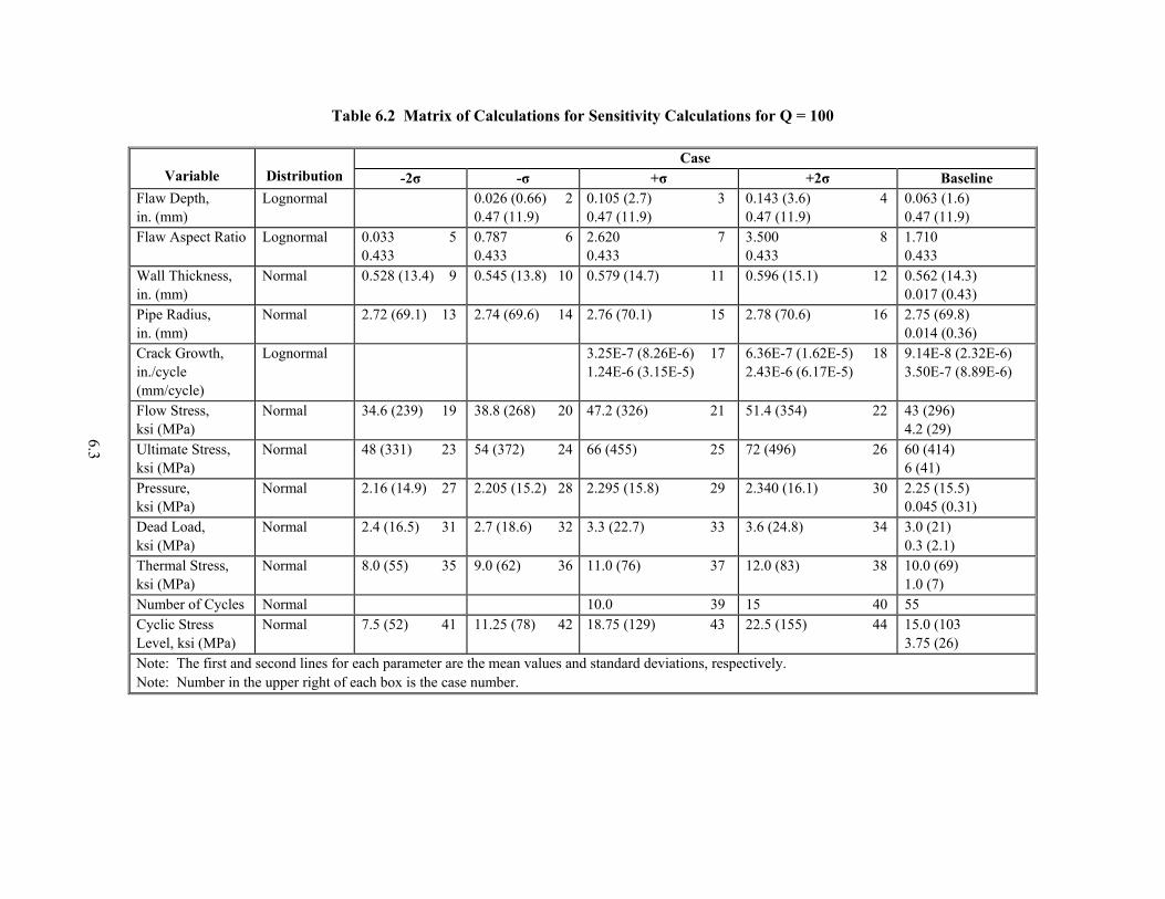
Table 6.2 Matrix of Calculations for or Q = 100
Case
Sensitivity Calculations f
Variable Distribution -2σ -σ +σ +2σ Baseline Fi
lan.
Lognormal 0.026 (0 20.47 (11.9)
0.105 (2.7) 3 0.47 (11.9)
0.143 (3.6) 4 0.47 (11.9)
0.063 (1.6) 0.47 (11.9)
w Depth, (mm)
.66)
Fla Logno 6 2. 7 0.
3.500 8 0.433
1.710 0.433
w Aspect Ratio rmal 0.030.43
3 3
5 0.0.
7843
73 620
433 Wan.
Normal 13. 54 0 0. 14.7) 0.596 (15.1) 12 0.562 (14.3) 0.017 (0.43)
ll Thickness, (mm) i
0.528 ( 4) 9 0. 5 (13.8) 1 579 ( 11
Pi
ipn.
Normal (69.1) 2.74 4 2. 0.1) 2.78 (70.6) 16 2.75 (69.8) 0.014 (0.36)
e Radius, (mm)
2.72 13 (69.6) 1 76 (7 15
Ci(
ran./m
Lognormal 3. 7 (8.26E-6) 1. 6 (3.15E-5)
6.36E-7 (1.62E-5) 18 2.43E-6 (6.17E-5)
9.14E-8 (2.32E-6) 3.50E-7 (8.89E-6)
ck Growth, cycle m/cycle)
25E-24E-
17
Fk
losi (M
Normal 47 26) 51.4 (354) 22 43 (296) 4.2 (29)
w Stress, Pa)
34.6 (239) 19 38.8 (268) 20 .2 (3 21
Uk
ltimasi (M
Normal 24 66 5) 72 (496) 26 60 (414) 6 (41)
te Stress, Pa)
48 (331) 23 54 (372) (45 25
Pk
ressursi (M
Normal ) 28 2. 15.8) 2.340 (16.1) 30 2.25 (15.5) 0.045 (0.31)
e, Pa)
2.16 (14.9) 27 2.205 (15.2 295 ( 29
Dk
ead Lsi (M
Normal 2 3. .7) 3.6 (24.8) 34 3.0 (21) 0.3 (2.1)
oad, Pa)
2.4 (16.5) 31 2.7 (18.6) 3 3 (22 33
Tk
hermsi (M
Normal 8.0 (55) 35 9.0 (62) 36 11 6) 12.0 (83) 38 10.0 (69) 1.0 (7)
al Stress, Pa)
.0 (7 37
Numb Normal 10 15 40 55 er of Cycles .0 39CL
yclic evel,
Normal 2 18 129) 22.5 (155) 44 15.0 (103 3.75 (26)
Stress ksi (MPa)
7.5 (52) 41 11.25 (78) 4 .75 ( 43
Note: cond lines for each parameter are the mean values an deviations spectively. Note: upper right of each box is the case number.
, red standardThe first and seNumber in the
6.3
A total of 44 cases was run for each of the three Q-factor values (Q = 1, 100, and 10,000). These three v ty stud 8 liters/min]) and break robabilities relative to the corresponding probabilities for the baseline case. These relative probabilities
arsampara
alculations indicated that leak probabilities were most sensitive to changes in the flaw depth, flaw-asof th rs of m
alues addressed a wide range of cyclic stresses and resulting failure probabilities. In the sensitiviies, the interest was in leak (with big leaks being > 100 gal/min [37
pe listed in the columns of Table 6.3 under the headings “Leak Ratio” and “LOCA Ratio,” with these
e ratios shown plotted in Figures 6.1 and 6.2. The probabilities are insensitive to changes in the meter if the ratio of probabilities is close to 1.
Cpect ratio, crack-growth rate, and level and number of cyclic stresses. The prescribed changes in some
ese parameters resulted in leak probabilities higher/lower than the baseline by as much as 2.5 ordeagnitude.
6.4
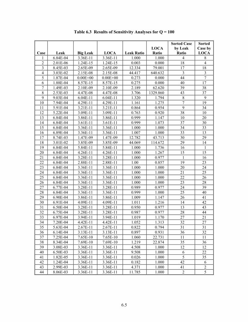
Table 6.3 Results of Sensitivity Analyses for Q = 100
Case Leak Big Leak LOCA Leak Ratio LOCA Ratio
Sorted Case by Leak
Ratio
Sorted Case by LOCA
1 6.84E-04 3.36E-11 3.36E-11 1.000 1.000 4 8 2 2.01E-06 1.24E-15 1.24E-15 0.003 0.000 18 4 3 8.45E-03 2.65E-09 2.65E-09 12.334 79.001 17 18 4 3.03E-02 2.15E-08 2.15E-08 44.417 640.632 3 3 5 1.87E-04 0.00E+00 0.00E+00 0.273 0.000 44 7 6 1.88E-04 8.57E-15 8.57E-15 0.275 0.000 40 17 7 1.49E-03 2.10E-09 2.10E-09 2.189 62.620 39 38 8 2.53E-03 4.47E-08 4.47E-08 3.706 1329.860 43 37 9 9.03E-04 6.04E-11 6.04E-11 1.320 1.794 8 9
10 7.94E-04 4.29E-11 4.29E-11 1.161 1.275 7 19 11 5.91E-04 3.21E-11 3.21E-11 0.864 0.954 9 34 12 5.22E-04 3.09E-11 3.09E-11 0.763 0.920 38 10 13 6.84E-04 3.86E-11 3.86E-11 0.999 1.147 10 20 14 6.84E-04 3.61E-11 3.61E-11 0.999 1.073 37 30 15 6.84E-04 3.36E-11 3.36E-11 1.000 1.000 34 33 16 6.89E-04 3.36E-11 3.36E-11 1.007 1.000 33 13 17 8.74E-03 1.47E-09 1.47E-09 12.782 43.713 30 29 18 3.01E-02 3.85E-09 3.85E-09 44.069 114.672 29 14 19 6.84E-04 5.84E-11 5.84E-11 1.000 1.736 16 1 20 1.000 1.267 15 15 6.84E-04 4.26E-11 4.26E-11 21 6.84E-04 3.28E-11 3.28E-11 1.000 0.977 1 16 22 6.84E-04 2.88E-11 2.88E-11 1.00 0.857 19 23 23 6.84E-04 3.36E-11 3.36E-11 1.000 1.000 20 24 24 6.84E-04 3.36E-11 3.36E-11 1.000 1.000 21 25 25 6.84E-04 3.36E-11 3.36E-11 1.000 1.000 22 26 26 .84E-04 3.36E-11 3.36E-11 1.000 1.000 23 28 627 6 0.989 0.977 24 39 .77E-04 3.28E-11 3.28E-1128 6.84E-04 3.36E-11 3.36E-11 0.999 1.000 25 40 29 6.90E-04 3.86E-11 3.86E-11 1.009 1.147 26 41 30 6.91E-04 4.09E-11 4.09E-11 1.011 1.216 14 42 31 6.50E-04 3.28E-11 3.28E-11 0.950 0.977 13 43 32 6.75E-04 3.28E-11 3.28E-11 0.987 0.977 28 44 33 6.97E-04 3.94E-11 3.94E-11 1.019 1.170 27 21 34 7.20E-04 4.42E-11 4.42E-11 1.052 1.313 32 27 35 5.63E-04 2.67E-11 2.67E-11 0.822 0.794 31 31 36 6.14E-04 3.13E-11 3.13E-11 0.897 0.931 36 32 37 7.25E-04 7.65E-10 7.65E-10 1.060 22.731 11 11 38 8.34E-04 7.69E-10 7.69E-10 1.219 22.874 35 36 39 3.08E-03 3.36E-11 3.36E-11 4.508 1.000 12 12 40 6.50E-03 3.36E-11 3.36E-11 9.508 1.000 6 22 41 1.82E-05 3.36E-11 3.36E-11 0.026 1.000 5 35 42 1.24E-04 3.36E-11 3.36E-11 0.182 1.000 42 6 43 2.99E-03 3.36E-11 3.36E-11 4.371 1.000 41 2 44 8.06E-03 3.36E-11 3.36E-11 11.785 1.000 2 5
6.5
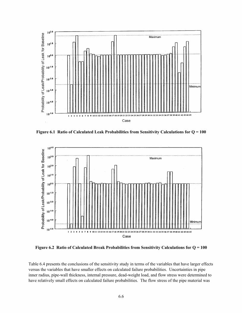
Figure 6.1 Ratio of Calculated Leak Probabilities from Sensitivity Calculations for Q = 100
Figure 6.2 Ratio of Calculated Break Probabilities from Se
nsitivity Calculations for Q = 100
study in terms of the variables that have larger effects
Table 6.4 presents the conclusions of the sensitivityversus the variables that have smaller effects on calculated failure probabilities. Uncertainties in pipe inner radius, pipe-wall thickness, internal pressure, dead-weight load, and flow stress were determined to have relatively small effects on calculated failure probabilities. The flow stress of the pipe material was
6.6
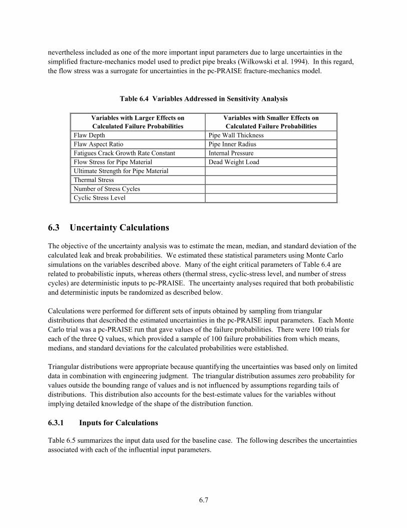
nevertheless included as one of the more important input parameters due to large uncertainties in the simplified fracture-mechanics model used to predict pipe breaks (Wilkowski et al. 1994). In this regathe flow stress was a surrogate for uncertainties in the pc-PRAISE fracture-mechanics model.
Table 6.4 Variables Addressed in Sensitivity Analysis
rd,
Variables with Larger Effects on Calculated Failure Probabilities
Variables with Smaller Effects on Calculated Failure Probabilities
Flaw Depth Pipe Wall Thickness Flaw Aspect Ratio Pipe Inner Radius Fatigues Crack Growth Rate Constant Internal Pressure Flow Stress for Pipe Material Dead Weight Load Ultimate Strength for Pipe Material Thermal Stress Number of Stress Cycles Cyclic Stress Level
6.3 Uncertainty Calculations
The objective of the uncertainty analysis was to estimate the mean, median, and standard deviation of the calculated leak and break probabilities. We estimated these statistical parameters using Monte Carlo simulations on the variables described above. Many of the eight critical parameters of Table 6.4 are related to probabilistic inputs, whereas others (thermal stress, cyclic-stress level, and number of stress cycles) are deterministic inputs to pc-PRAISE. The uncertainty analyses required that both probabilistic and deterministic inputs be randomized as described below. Calculations were performed for different sets of inputs obtained by sampling from triangular distributions that described the estimated uncertainties in the pc-PRAISE input parameters. Each Monte Carlo trial was a pc-PRAISE run that gave values of the failure probabilities. There were 100 trials for each of the three Q values, which provided a sample of 100 failure probabilities from which means, medians, and standard deviations for the calculated probabilities were established. Triangular distributions were appropriate because quantifying the uncertainties was based only on limited data in combination with engineering judgment. The triangular distribution assumes zero probability for values outside the bounding range of values and is not influenced by assumptions regarding tails of distributions. This distribution also accounts for the best-estimate values for the variables without implying detailed knowledge of the shape of the distribution function. 6.3.1 Inputs for Calculations
Table 6.5 summarizes the input data used for the baseline case. The following describes the uncertainties associated with each of the influential input parameters.
6.7
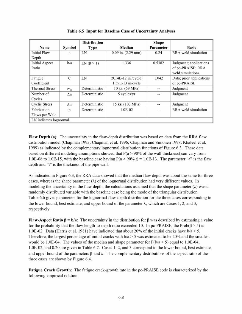
Table 6.5 Input for Baseline Case of Uncertainty Analyses
Name Symbol Distribution
Type Median Shape
Parameter Basis
Initial Flaw Depth
a LN 0.09 in. (2.29 mm) 0.24 RRA weld simulation
Initial Aspect Ratio
b/a LN (β > 1) 1.336 0.5382 Judgment; applications of pc-PRAISE; RRA weld simulations
Fatigue Coefficient
C LN (9.14E-12 in./cycle) 1.59E-13 m/cycle
1.042 Data; prior applications of pc-PRAISE
Thermal Stress σth Deterministic 10 ksi (69 MPa) -- Judgment Number of Cycles
∆n Deterministic 5 cycles/yr -- Judgment
Cyclic Stress ∆σ Deterministic 15 ksi (103 MPa) -- Judgment Fabrication Flaws per Weld
p Deterministic 1.0E-02 -- RRA weld simulation
LN indicates lognormal. Flaw Depth (a): The uncertainty in the flaw-depth distribution was based on data from the RRA flaw distribution model (Chapman 1993; Chapman et al. 1996; Chapman and Simonen 1998; Khaleel et al. 1999) as indicated by the complementary lognormal distribution functions of Figure 6.3. These data based on different modeling assumptions showed that P(a > 90% of the wall thickness) can vary from 1.0E-08 to 1.0E-15, with the baseline case having P(a > 90% t) = 1.0E-13. The parameter “a” is the flaw depth and “t” is the thickness of the pipe wall. As indicated in Figure 6.3, the RRA data showed that the median flaw depth was about the same for three cases, whereas the shape parameter (λ) of the lognormal distribution had very different values. In modeling the uncertainty in the flaw depth, the calculations assumed that the shape parameter (λ) was a randomly distributed variable with the baseline case being the mode of the triangular distribution. Table 6.6 gives parameters for the lognormal flaw-depth distribution for the three cases corresponding to the lower bound, best estimate, and upper bound of the parameter λ, which are Cases 1, 2, and 3, respectively. Flaw-Aspect Ratio β = b/a: The uncertainty in the distribution for β was described by estimating a value for the probability that the flaw length-to-depth ratio exceeded 10. In pc-PRAISE, the Prob(β > 5) is 1.0E-02. Data (Harris et al. 1981) have indicated that about 20% of the initial cracks have b/a > 5. Therefore, the largest percentage of initial cracks with b/a > 5 was estimated to be 20% and the smallest would be 1.0E-04. The values of the median and shape parameter for P(b/a > 5) equal to 1.0E-04, 1.0E-02, and 0.20 are given in Table 6.7. Cases 1, 2, and 3 correspond to the lower bound, best estimate, and upper bound of the parameters β and λ. The complementary distributions of the aspect ratio of the three cases are shown by Figure 6.4. Fatigue Crack Growth: The fatigue crack-growth rate in the pc-PRAISE code is characterized by the following empirical relation:
6.8
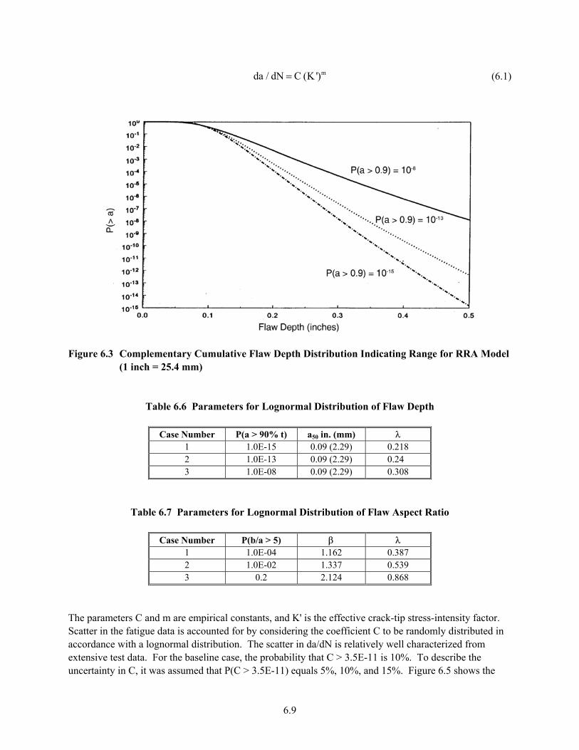
(6.1)
mda / dN C (K ')=
Figure 6.3 Complementary Cumulative Flaw Depth Distribution Indicating Range for RRA Mod
(1 inch = 25.4 mm)
Table 6.6 Parameters for Lognormal Distribution of Flaw Depth
el
Case Number P(a > 90% t) a50 in. (mm) λ
1 1.0E-15 0.09 (2.29) 0.218 2 1.0E-13 0.09 (2.29) 0.24 3 1.0E-08 0.09 (2.29) 0.308
Table 6.7 Parameters for Lognormal Distribution of Flaw Aspect Ratio
Case Number P(b/a > 5) β λ 1 1.0E-04 1.162 0.387 2 1.0E-02 1.337 0.539 3 0.2 2.124 0.868
T constants, and K' is the effective crack-tip stress-intensity factor.
y considering the coefficient C to be randomly distributed in ccordance with a lognormal distribution. The scatter in da/dN is relatively well characterized from
extensive test data. For the baseline case, the probability that C > 3.5E-11 is 10%. To describe the uncertainty in C, it was assumed that P(C > 3.5E-11) equals 5%, 10%, and 15%. Figure 6.5 shows the
he parameters C and m are empirical Scatter in the fatigue data is accounted for ba
6.9
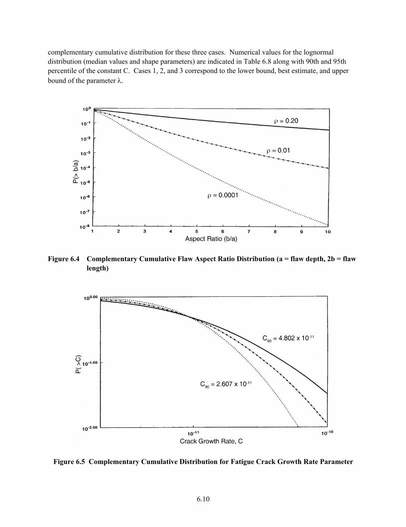
complementary cumulative distribution for these three cases. Numerical values for the lognormal distribution (median values and shape parameters) are indicated in Table 6.8 along with 90th and 95th percentile of the constant C. Cases 1, 2, and 3 correspond to the lower bound, best estimate, and upper
ound of the parameter λ.
b
Figure 6.4 Complementary Cumulative Flaw Aspect Ratio Distribution (a = flaw depth, 2
length)
b = flaw
Figure 6.5 Complementary Cumulative Distribution for Fatigue Crack Growth Rate Parameter
6.10
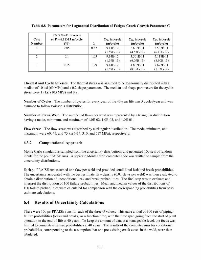
Table 6.8 Parameters for Lognormal Distribution of Fatigue Crack Growth Parameter C
P > Case
3.5E-11 in./cycle or P > 6.1E-13 m/cycle C50, in./cycle C90, in./cycle C95, in./cycle
Number (%) λ (m/cycle) (m/cycle) (m/cycle) 1 0.05 0.82 9.14E-12
(1.59E-13) 2.607E-11 (4.53E-13)
3.507E-11 (6.10E-13)
2 0.1 1.05 9.14E-12 (1.59E-13)
3.501E-11 (6.09E-13)
5.118E-11 (8.90E-13)
3 0.15 1.29 9.14E-12 4.802E-11 7.677E(1.59E-13) (8.35E-13)
-11 (1.33E-12)
Thermal and Cyclic Stresses: The thermal stress was assumed to be lognormally distributed with a median of 10 ksi (69 MPa) and a 0.2 shape parameter. The median and shape parameters for the cyclic tress were 15 ksi (103 MPa) and 0.2. s
Number of Cycles: The number of cycles for every year of the 40-year life was 5 cycles/year and was assumed to follow Poisson’s distribution.
umber of Flaws/Weld: The number of flaws per weld was represented by a triangular distN ribution
s. est estimate flaw density (0.01 flaws per weld) was then evaluated to
The final step was to evaluate and
f piping-t
having a mode, minimum, and maximum of 1.0E-02, 1.0E-03, and 1.0E-01. Flow Stress: The flow stress was described by a triangular distribution. The mode, minimum, and maximum were 60, 45, and 75 ksi (414, 310, and 517 MPa), respectively. 6.3.2 Computational Approach
Monte Carlo simulations sampled from the uncertainty distributions and generated 100 sets of random inputs for the pc-PRAISE runs. A separate Monte Carlo computer code was written to sample from the uncertainty distributions. Each pc-PRAISE run assumed one flaw per weld and provided conditional leak and break probabilitie
he uncertainty associated with the bTobtain a distribution of unconditional leak and break probabilities. interpret the distribution of 100 failure probabilities. Mean and median values of the distributions of 100 failure probabilities were calculated for comparison with the corresponding probabilities from best-estimate calculations. 6.4 Results of Uncertainty Calculations
here were 100 pc-PRAISE runs for each of the three Q values. This gave a total of 300 sets oTfailure probabilities (leaks and breaks) as a function time, with the time span going from the start of planoperation to the end-of-life at 40 years. To keep the amount of data at a manageable level, the focus waslimited to cumulative failure probabilities at 40 years. The results of the computer runs for conditional probabilities, corresponding to the assumption that one pre-existing crack exists in the weld, were then tabulated.
6.11
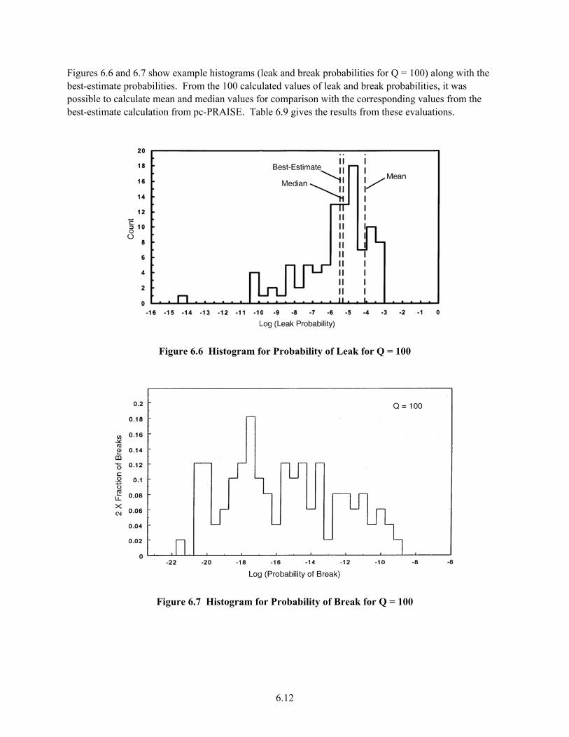
Figures 6.6 and 6.7 show example histograms (leak and break probabilities for Q = 100) along with the
posest-estimate calculation from pc-PRAISE. Table 6.9 gives the results from these evaluations.
best-estimate probabilities. From the 100 calculated values of leak and break probabilities, it was sible to calculate mean and median values for comparison with the corresponding values from the
b
Figure 6.6 Histogram for Probability of Leak for Q = 100
Figure 6.7 Histogram for Probability of Break for Q = 100
6.12
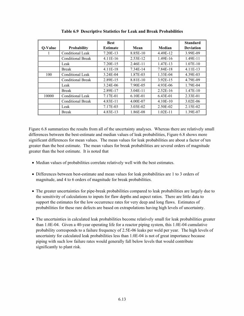
Table 6.9 Descriptive Statistics for Leak and Break Probabilities
Q-Value Probability Mean Standard Deviation
Best Estimate Median
1 Cond 13 4. itional Leak 7.20E- 8.85E-10 49E-12 3.99E-09 Condi k 6 1 1tional Brea 4.11E-1 2.53E-12 .49E-16 .49E-11 Leak 5 1 17.20E-1 2.46E-11 .47E-13 .07E-10 Break 8 7 4 4.11E-1 7.34E-14 .84E-18 .11E-13
100 Condi 1 4tional Leak 3.24E-04 1.87E-03 .33E-04 .39E-03 Condi k 5 3 4tional Brea 2.89E-1 8.81E-10 .92E-15 .79E-09 Leak 6 4 13.24E-0 7.90E-05 .93E-06 .79E-04 Break 7 2 1 2.89E-1 3.04E-11 .52E-16 .47E-10
10000 Condi 6 2tional Leak 7.17E-01 6.10E-01 .43E-01 .33E-01 Condi k 1 4 3tional Brea 4.83E-1 4.00E-07 .10E-10 .02E-06 Leak 3 2 27.17E-0 3.03E-02 .50E-02 .15E-02 Break 3 1 1 4.83E-1 1.86E-08 .02E-11 .39E-07
Figure 6.8 summarizes the results from all of the uncerta es. W re are differenc een the ate and values obabil re 6.8 significa ences fo lues. The mean value probab about ten greater than the best esti mean values for break probabilities are several orders of mgreater than the best esti s noted • Median values of probabili well with the best estim tes.
trapolations having high levels of uncertainty.
eak probabilities less than 1.0E-04 is not of great importance because piping with such low failure rates would generally fall below levels that would contribute significantly to plant risk.
inty analys hereas the relatively small es betw best-estim median of leak pr ities, Figu shows more nt differ r mean va s for leak ilities are a factor of
mate. The agnitude mate. It i that
ties correlate relatively a • Differences between best-estimate and mean values for leak probabilities are 1 to 3 orders of
magnitude, and 4 to 6 orders of magnitude for break probabilities. • The greater uncertainties for pipe-break probabilities compared to leak probabilities are largely due to
the sensitivity of calculations to inputs for flaw depths and aspect ratios. There are little data to support the estimates for the low occurrence rates for very deep and long flaws. Estimates of probabilities for these rare defects are based on ex
• The uncertainties in calculated leak probabilities become relatively small for leak probabilities greater
than 1.0E-04. Given a 40-year operating life for a reactor piping system, this 1.0E-04 cumulative probability corresponds to a failure frequency of 2.5E-06 leaks per weld per year. The high levels of uncertainty for calculated l
6.13
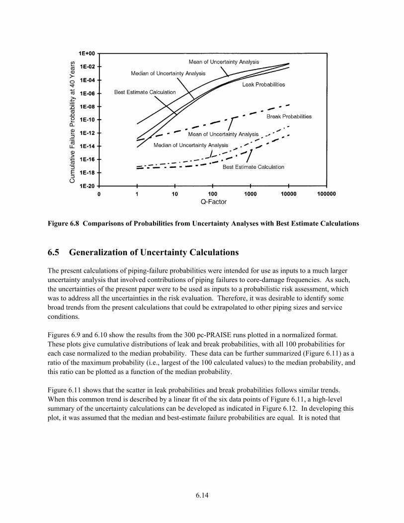
Figure 6.8 Comparisons of Probabilities from Unce ty Analyse Estimate Calculations 6.5 Generalization of Uncertainty Calculations
The present calculations of piping-failure probabilities intended fo uts to a much larger uncertainty analysis that involved contributions of pipi ilures to cor requencies. As such, the uncertainties of the present paper were to be used as inputs to a probabilistic risk assessment, which was to address all the uncertainties in the risk evaluatio herefore, it e broad trends from the present calculations that could b apolated to g sizes and service conditions. Figures 6.9 and 6.10 show the results from the 300 pc SE runs plo rmalized format. These plots give cumulative distributions of leak and probabilities, with all 100 probabilities for each case normalized to the probability. Thes can be furt ized (Figure 6.11) as a
tio of the maximum probabilit rgest of the 100 calculated values) to the median probability, and is ratio can be plotted as a function of the median probability.
s and break probabilities follows similar trends.
his
rtain s with Best
were r use as inpng fa e-damage f
n. T was desirable to identify some extr other pipin
-PRAI tted in a nobreak
mediany (i.e., la
e data her summarrath Figure 6.11 shows that the scatter in leak probabilitieWhen this common trend is described by a linear fit of the six data points of Figure 6.11, a high-level summary of the uncertainty calculations can be developed as indicated in Figure 6.12. In developing tplot, it was assumed that the median and best-estimate failure probabilities are equal. It is noted that
6.14
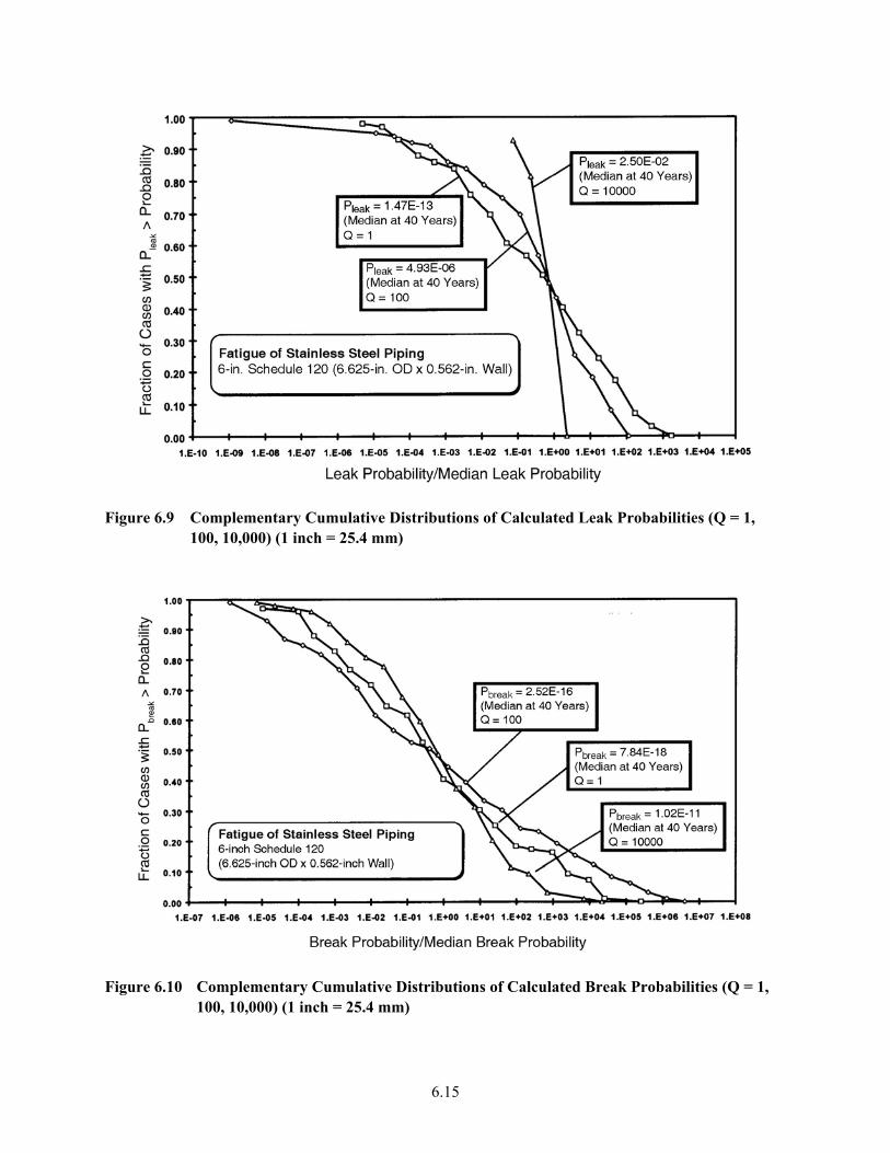
igure 6.9 Complementary Cumulative Distributions of Calculated Leak Probabilities (Q = 1, F100, 10,000) (1 inch = 25.4 mm)
Figure 6.10 Complementary Cumulative Distributions of Calculated Break Probabilities (Q = 1,
100, 10,000) (1 inch = 25.4 mm)
6.15
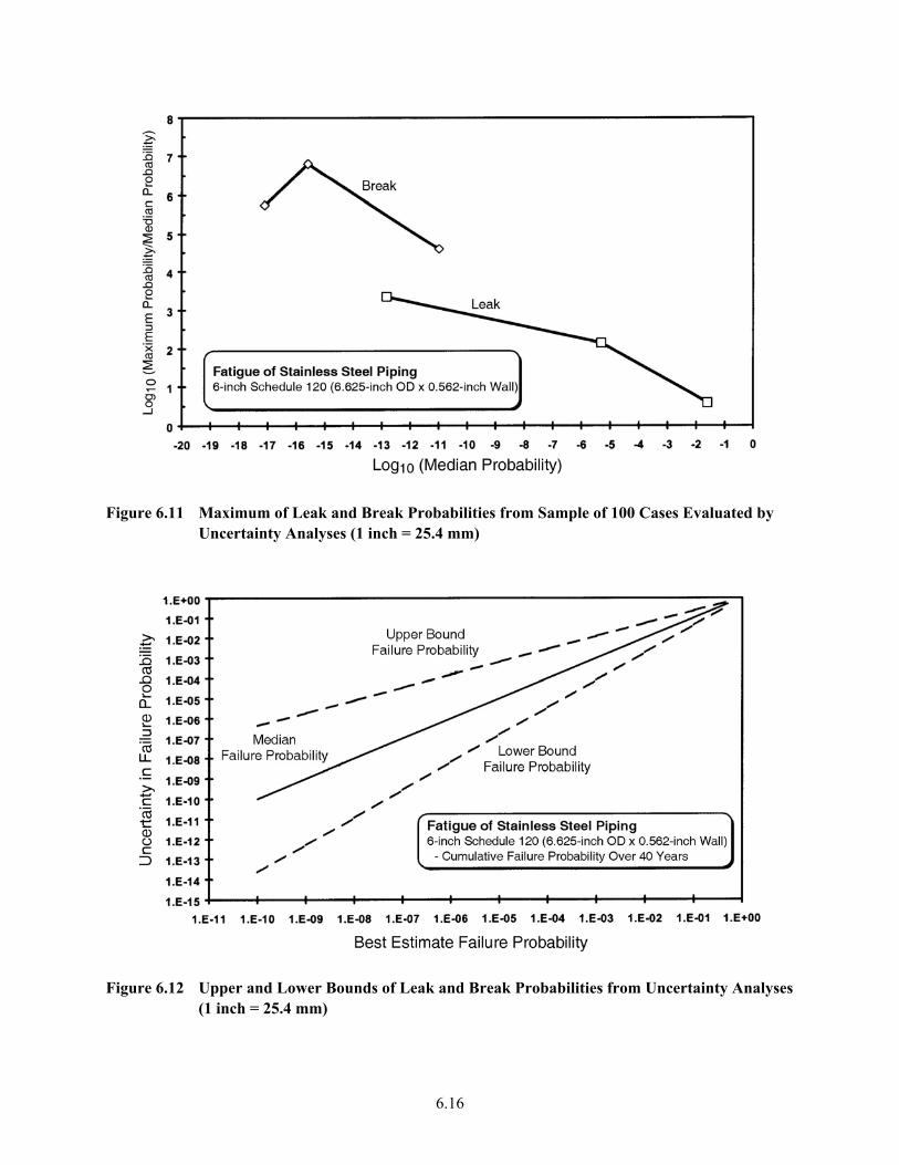
igure 6.11 Maximum of Leak and Break Probabilities from Sample of 100 Cases Evaluated by Uncertainty Analyses (1 inch = 25.4 mm)
F
Figure 6.12 Upper and Lower Bounds of Leak and Break Probabilities from Uncertainty Analyses
(1 inch = 25.4 mm)
6.16
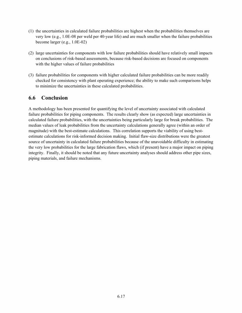
(1) the uncertainties in calculated failure probabilities are highest when the probabilities themselves ar (e.g., 1.0E-08 per weld per 40-year life) and ar
e very low e much smaller when the failure probabilities become larger (e.g., 1.0E-02)
(2) large uncertainties for components with low failure probabilities should have relatively small impacts on conclusions of risk-based assessments, because risk-based decisions are focused on components with the higher values of failure probabilities
(3) failure probabilities for components with higher calculated failure probabilities can be more readily
checked for consistency with plant operating experience; the ability to make such comparisons helps to minimize the uncertainties in these calculated probabilities.
6.6 Conclusion
A methodology has been presented for quantifying the level of uncertainty associated with calculated failure probabilities for piping components. The results clearly show (as expected) large uncertainties in calculated failure probabilities, with the uncertainties being particularly large for break probabilities. The median values of leak probabilities from the uncertainty calculations generally agree (within an order of magnitude) with the best-estimate calculations. This correlation supports the viability of using best-estimate calculations for risk-informed decision making. Initial flaw-size distributions were the greatest ource of uncertainty in calculated failure probabilities because of the unavoidable difficulty in es mating
ping integrity. Fin nty analyses should address other pipe sizes,
iping materials, and failure mechanisms.
s tithe very low probabilities for the large fabrication flaws, which (if present) have a major impact on pi
ally, it should be noted that any future uncertaip
6.17

6.18
7 Effects of Flaw-Sizing Errors on the Reliability of
rs. lues of flaw-detection probability, flaw-sizing errors, and
ac
.
d
ity s are performed. Significant undersizing
f flaws could cause incorrect repair decisions. In some cases flaws could be incorrectly classified as benign if their measured sizes are less than the sizes of the governing flaw-acceptance criteria. This section describes calculations that address flaw-sizing errors in numerical simulations of alternative inspection scenarios. These calculations are applicable to mechanical and thermal fatigue of stainless steel piping. In addition to flaw-sizing errors, the uncertainties addressed in the PFM model are • the numbers of initial flaws • the distribution of flaw sizes • the crack growth rates for the flaws • POD curves • frequency of the inspection • flaw-acceptance criteria.
Vessels and Piping
7.1 Introduction
The nuclear power industry has continued to upgrade the quality of UT inspections by addressing the key elements needed for effective inspections, namely personnel, procedures, and equipment. Central to theseefforts has been the qualification of inspection teams before field inspections, whereby the teams must demonstrate acceptable performance in detecting and sizing defects during trial inspections of degraded piping samples. These efforts have resulted in significant enhancement of inservice inspection (ISI) ffectiveness through changes to ASME Section XI Code, Appendix VIII (Cowfer 1989). e
This section describes PFM calculations that simulate fatigue crack growth, flaw detection, flaw-sizing accuracy, and the impacts of flaw-acceptance criteria. A numerical implementation based on a Latin Hypercube approach was applied in calculations, which have been performed for a range of paramete
hese were used to obtain representative vaTflaw- ceptance criteria. Performance demonstrations have addressed two measures of NDE reliability-POD and flaw-sizing accuracy. Both measures impact the ability of an inspection program to enhance the reliability of pipingPrevious papers by the present authors (Woo and Simonen 1984; Simonen 1990; Khaleel and Simonen 1994a, 1994b, 1995; Khaleel et al. 1995) have described PFM calculations that have evaluated the impactinspections with various POD levels (i.e., POD as a function of flaw size) on the ability of inservice anpreservice inspections to reduce leak and rupture probabilities of reactor piping. Flaw detection with a high level of reliability is an important step to ensure that ISIs will reduce the failure probabilities of the inspected piping locations. However, inspections can impact piping reliabilonly if the detected flaws are repaired or other corrective actiono
7.1
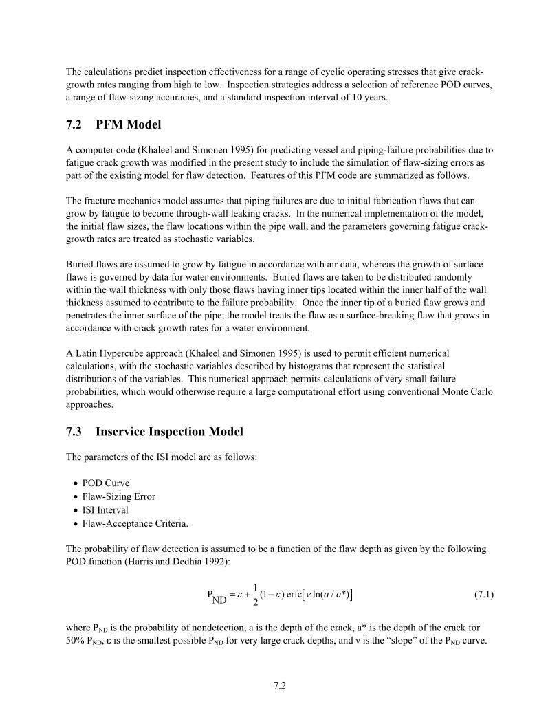
The calculations predict inspection effectiveness for a ange of cyclic operating stresses that give crack-rowth rates ranging from high to low. Inspection strategies address a selection of reference POD curves,
.2 PFM Model
A computer code (Khaleel and Simonen 1995) for predicting vessel and piping-failure probabilities due to fatigue crack growth was modified in the present study to include the simulation of flaw-sizing errors as part of the existing model for flaw detection. Features of this PFM code are summarized as follows. The fracture mechanics model assumes that piping failures are due to initial fabrication flaws that can grow by fatigue to become through-wall leaking cracks. In the numerical implementation of the model, the initial flaw sizes, the flaw locations within the pipe wall, and the parameters governing fatigue crack-growth rates are treated as stochastic variables. Buried flaws are assumed to grow by fatigue in accordance with air data, whereas the growth of surface flaws is governed by data for water environments. Buried flaws are taken to be distributed randomly within the wall thickness with only those flaws having inner tips located within the inner half of the wall thickness assumed to contribute to the failure probability. Once the inner tip of a buried flaw grows and penetrates the inner surface of the pipe, the model treats the flaw as a surface-breaking flaw that grows in accordance with crack growth rates for a water environment.
percube approach (Khaleel and Simonen 1995) is used to permit efficient numerical ,
robabilities, ing conventional Monte Carlo pproaches.
.3 Inservice Inspection Model
The parameters of the ISI model are as follows:
• POD Curve • Flaw-Sizing Error • ISI Interval • Flaw-Acceptance Criteria.
The probability of flaw detection is assumed to be a function of the flaw depth as given by the following POD function (Harris and Dedhia 1992):
rga range of flaw-sizing accuracies, and a standard inspection interval of 10 years.
7
A Latin Hycalculations with the stochastic variables described by histograms that represent the statistical distributions of the variables. This numerical approach permits calculations of very small failure
which would otherwise require a large computational effort uspa 7
[ ]1P (1 ) erfc ln( /ND 2a aε ε ν= + − *) (7.1)
where PND is the probability of nondetection, a is the depth of the crack, a* is the depth of the crack for 50% PND, ε is the smallest possible PND for very large crack depths, and ν is the “slope” of the PND curve.
7.2
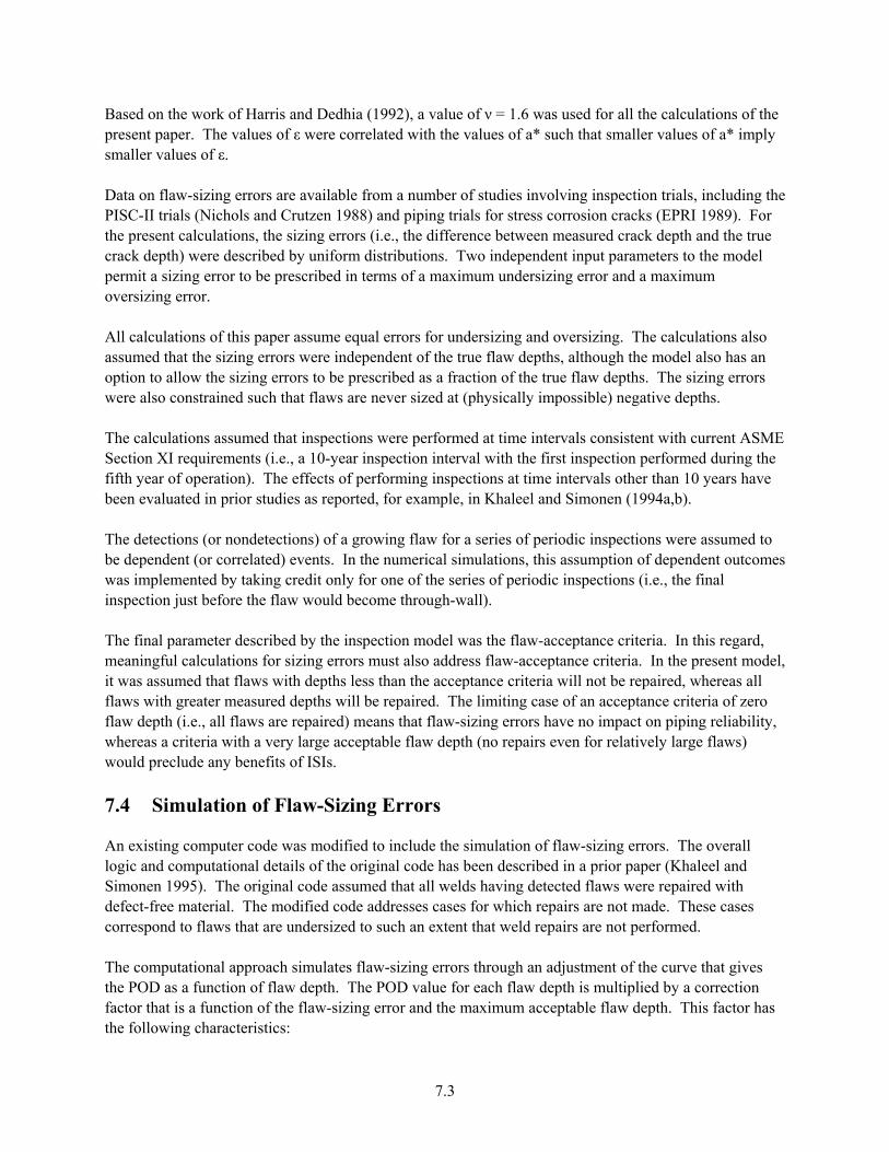
Based on the work of Harris and Dedhia (1992), a value of ν = 1.6 was used for all the calculations of the present paper. The values of ε were correlated with the values of a* such that smaller values of a* imply smaller values of ε. Data on flaw-sizing errors are available from a number of studies involving inspection trials, including the PISC-II trials (Nichols and Crutzen 1988) and piping trials for stress corrosion cracks (EPRI 1989). For the present calculations, the sizing errors (i.e., the difference between measured crack depth and the true crack depth) were described by uniform distributions. Two independent input parameters to the model permit a sizing error to be prescribed in terms of a maximum undersizing error and a maximum oversizing error. All calculations of this paper assume equal errors for undersizing and oversizing. The calculations also assumed that the sizing errors were independent of the true flaw depths, although the model also has an option to allow the sizing errors to be prescribed as a fraction of the true flaw depths. The sizing errors were also constrained such that flaws are never sized at (physically impossible) negative depths. The calculations assumed that inspections were performed at time intervals consistent with current ASME
ection XI requirements (i.e., a 10-year inspection interval with the first inspection performed during the
been evaluat onen (1994a,b).
The detections (or nondetections) of a growing flaw for a series of periodic inspections were assumed to be dependent (or correlated) events. In the numerical simulations, this assumption of dependent outcomes was implemented by taking credit only for one of the series of periodic inspections (i.e., the final inspection just before the flaw would become through-wall). The final parameter described by the inspection model was the flaw-acceptance criteria. In this regard, meaningful calculations for sizing errors must also address flaw-acceptance criteria. In the present model, it was assumed that flaws with depths less than the acceptance criteria will not be repaired, whereas all flaws with greater measured depths will be repaired. The limiting case of an acceptance criteria of zero flaw depth (i.e., all flaws are repaired) means that flaw-sizing errors have no impact on piping reliability, whereas a criteria with a very large acceptable flaw depth (no repairs even for relatively large flaws) would preclude any benefits of ISIs. 7.4 Simulation of Flaw-Sizing Errors
An existing computer code was modified to include the simulation of flaw-sizing errors. The overall logic and computational details of the original code has been described in a prior paper (Khaleel and Simonen 1995). The original code assumed that all welds having detected flaws were repaired with defect-free material. The modified code addresses cases for which repairs are not made. These cases correspond to flaws that are undersized to such an extent that weld repairs are not performed. The computational approach simulates flaw-sizing errors through an adjustment of the curve that gives the POD as a function of flaw depth. The POD value for each flaw depth is multiplied by a correction factor that is a function of the flaw-sizing error and the maximum acceptable flaw depth. This factor has the following characteristics:
Sfifth year of operation). The effects of performing inspections at time intervals other than 10 years have
ed in prior studies as reported, for example, in Khaleel and Sim
7.3
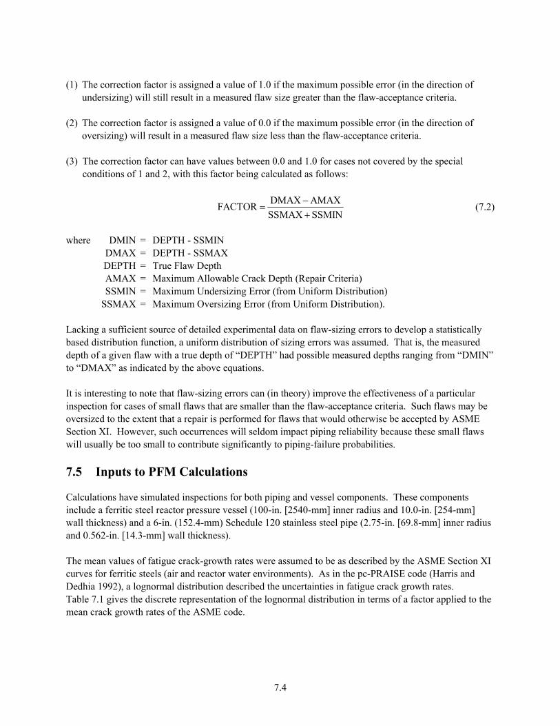
(1) The correction factor is assigned a value of 1.0 if the maximum possible error (in the direction of
undersizing) will still result in a measured flaw size greater than the flaw-acceptance criteria. (2) The correction factor is assigned a value of 0.0 if the maximum possible error (in the direction of
oversizing) will result in a measured flaw size less than the flaw-acceptance criteria. (3) The correction factor can have values between 0.0 and 1.0 for cases not covered by the special
conditions of 1 and 2, with this factor being calculated as follows:
DMAX AMAXFACTORSSMAX SSMIN
−=
+ (7.2)
where DMIN = DEPTH - SSMIN DMAX = DEPTH - SSMAX DEPTH = True Flaw Depth AMAX = Maximum Allowable Crack Depth (Repair Criteria) SSMIN = Maximum Undersizing Error (from Uniform Distribution) SSMAX = Maximum Oversizing Error (from Uniform Distribution). Lacking a sufficient source of detailed experimental data on flaw-sizing errors to develop a statistically based distribution function, a uniform distribution of sizing errors was assumed. That is, the measured depth of a given flaw with a true depth of “DEPTH” had possible measured depths ranging from “DMIN” to “DMAX” as indicated by the above equations. It is interesting to note that flaw-sizing errors can (in theory) improve the effectiveness of a particular inspection for cases of small flaws that are smaller than the flaw-acceptance criteria. Such flaws may be oversized to the extent that a repair is performed for flaws that would otherwise be accepted by ASME Section XI. However, such occurrences will seldom impact piping reliability because these small flaws will usually be too small to contribute significantly to piping-failure probabilities. 7.5 Inputs to PFM Calculations
Calculations have simulated inspections for both piping and vessel components. These components include a ferritic steel reactor pressure vessel (100-in. [2540-mm] inner radius and 10.0-in. [254-mm] wall thickness) and a 6-in. (152.4-mm) Schedule 120 stainless steel pipe (2.75-in. [69.8-mm] inner radius and 0.562-in. [14.3-mm] wall thickness). The mean values of fatigue crack-growth rates were assumed to be as described by the ASME Section XI curves for ferritic steels (air and reactor water environments). As in the pc-PRAISE code (Harris and Dedhia 1992), a lognormal distribution described the uncertainties in fatigue crack growth rates. Table 7.1 gives the discrete representation of the lognormal distribution in terms of a factor applied to the mean crack growth rates of the ASME code.
7.4
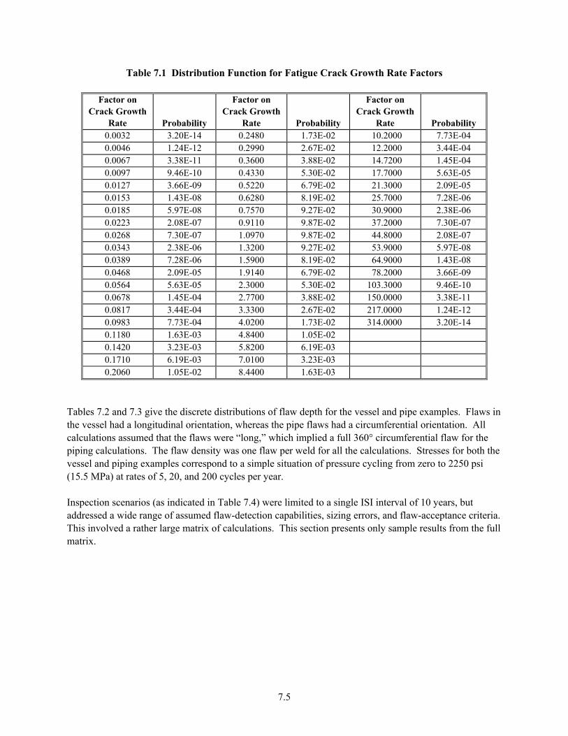
Table 7.1 Distribution Function for Fatigue Crack Growth Rate Factors
Factor on Factor on Factor on Crack Growth
Rate Probability Crack Growth
Rate Probability Crack Growth
Rate Probability 0.0032 3.20E-14 0.2480 1.73E-02 10.2000 7.73E-04 0.0046 1.24E-12 0.2990 2.67E-02 12.2000 3.44E-04 0.0067 3.38E-11 0.3600 3.88E-02 14.7200 1.45E-04 0.0097 9.46E-10 0.4330 5.30E-02 17.7000 5.63E-05 0.0127 3.66E-09 0.5220 6.79E-02 21.3000 2.09E-05 0.0153 1.43E-08 0.6280 8.19E-02 25.7000 7.28E-06 0.0185 5.97E-08 0.7570 9.27E-02 30.9000 2.38E-06 0.0223 2.08E-07 0.9110 9.87E-02 37.2000 7.30E-07 0.0268 7.30E-07 1.0970 9.87E-02 44.8000 2.08E-07 0.0343 2.38E-06 1.3200 9.27E-02 53.9000 5.97E-08 0.0389 7.28E-06 1.5900 8.19E-02 64.9000 1.43E-08 0.0468 2.09E-05 1.9140 6.79E-02 78.2000 3.66E-09 0.0564 5.63E-05 2.3000 5.30E-02 103.3000 9.46E-10 0.0678 1.45E-04 2.7700 3.88E-02 150.0000 3.38E-11 0.0817 3.44E-04 3.3300 2.67E-02 217.0000 1.24E-12 0.0983 7.73E-04 4.0200 1.73E-02 314.0000 3.20E-14 0.1180 1.63E-03 4.8400 1.05E-02 0.1420 3.23E-03 5.8200 6.19E-03 0.1710 6.19E-03 7.0100 3.23E-03 0.2060 1.05E-02 8.4400 1.63E-03
Tab ws in he n, whereas the pipe flaws had a circumferential orientation. All
ves(15 Inspadd teria. Thi sample results from the full
atrix.
les 7.2 and 7.3 give the discrete distributions of flaw depth for the vessel and pipe examples. Flavessel had a longitudinal orientatiot
calculations assumed that the flaws were “long,” which implied a full 360° circumferential flaw for the piping calculations. The flaw density was one flaw per weld for all the calculations. Stresses for both the
sel and piping examples correspond to a simple situation of pressure cycling from zero to 2250 psi .5 MPa) at rates of 5, 20, and 200 cycles per year.
ection scenarios (as indicated in Table 7.4) were limited to a single ISI interval of 10 years, but ressed a wide range of assumed flaw-detection capabilities, sizing errors, and flaw-acceptance cris involved a rather large matrix of calculations. This section presents only
m
7.5
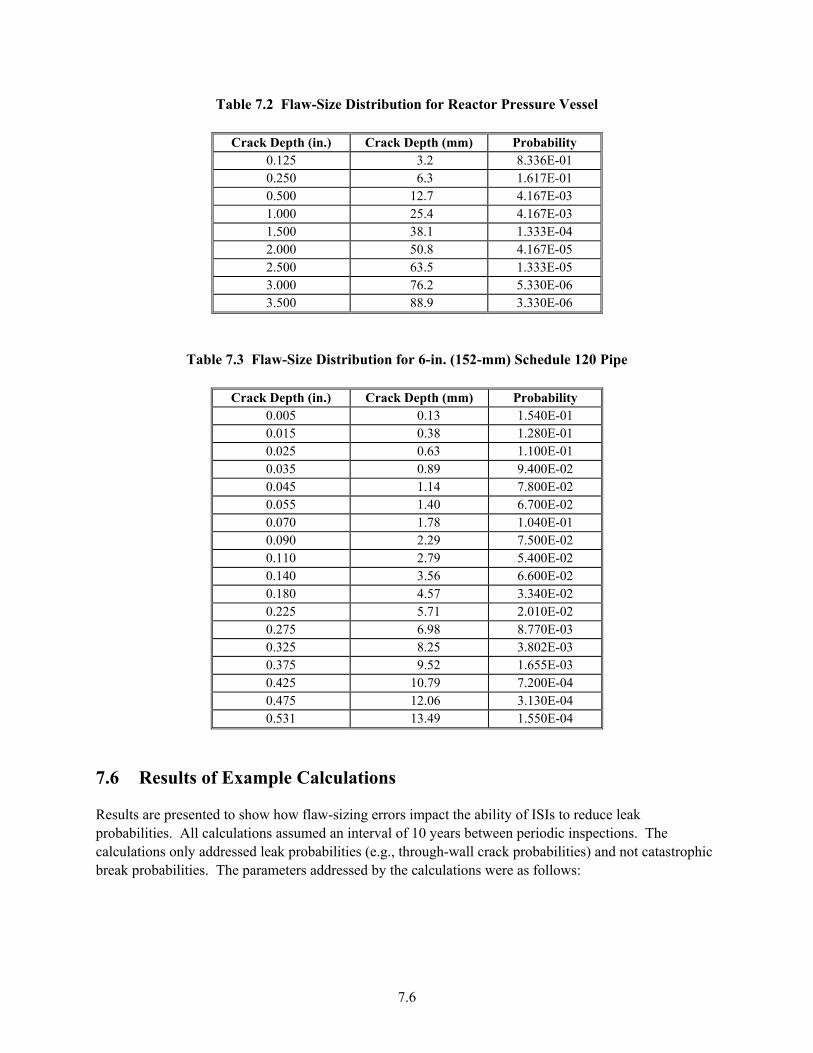
Table 7.2 Flaw-Size Distribution for Reactor Pressure Vessel
Crack Depth (in.) Crack Depth (mm) Probability
0.125 3.2 8.336E-01 0.250 6.3 1.617E-01 0.500 12.7 4.167E-03 1.000 25.4 4.167E-03 1.500 38.1 1.333E-04 2.000 50.8 4.167E-05 2.500 63.5 1.333E-05 3.000 76.2 5.330E-06 3.500 88.9 3.330E-06
Table 7.3 Flaw-Size Distribution for 6-in. (152-mm) Schedule 120 Pipe
Crack Depth (in.) Crack Depth (mm) Probability 0.005 0.13 1.540E-01 0.015 0.38 1.280E-01 0.025 0.63 1.100E-01 0.035 0.89 9.400E-02 0.045 1.14 7.800E-02 0.055 1.40 6.700E-02 0.070 1.78 1.040E-01 0.090 2.29 7.500E-02 0.110 2.79 5.400E-02 0.140 3.56 6.600E-02 0.180 4.57 3.340E-02 0.225 5.71 2.010E-02 0.275 6.98 8.770E-03 0.325 8.25 3.802E-03 0.375 9.52 1.655E-03 0.425 10.79 7.200E-04 0.475 12.06 3.130E-04 0.531 13.49 1.550E-04
7.6 Results of Example Calculations
Results are presented to show how flaw-sizing errors impact the ability of ISIs to reduce leak probabilities. All calculations assumed an interval of 10 years between periodic inspections. The calculations only addressed leak probabilities (e.g., through-wall crack probabilities) and not catastrophic break probabilities. The parameters addressed by the calculations were as follows:
7.6
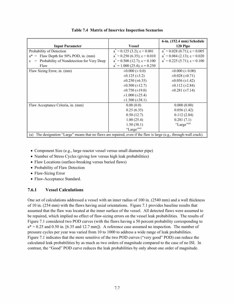
Table 7.4 Mat o tion Scenarios
6-in. (152.4 mm) Schedule
rix f Inservice Inspec
Input Parameter Vessel 120 Pipe Probability of Detection a* = 0.125 (3.2); ε = 0.001
*a*
a* = Flaw Depth for 50% POD, in. (mm) a = 0.250 (6.35); ε = 0.010 = 0.028 (0.71); ε = 0.005
a* = 0.084 (2.13); ε = 0.020 0 ε = Probability of Nondetection for Very Deep
Flaw a* = 0.500 (12.7); ε = 0.100 a* = 1.000 (25.4); ε = 0.250
a* = 0.225 (5.71); ε = 0.10
Flaw Sizing Error, in. (mm) ±0.000 (± 0.0) ±0.125 (±3.2)
±0.000 (± 0.00)
±0.250 (±6.35) ±0.500 (±12.7) ±0.750 (±19.0) ±1.000 (±25.4)
±0.056 (±1.42)±0.112 (±2.84) ±0.281 (±7.14)
±1.500 (±38.1)
±0.028 (±0.71)
Flaw Acceptance Criteria, in. (mm) 0.00 (0.0) 0.25 (6.35)
0.000 (0.00) 0.056 (1.42)
0.50 (12.7) 1.00 (25.4)
0.112 (2.84) 0.281 (7.1)
1.50 (38.1) “Large”(a)
“Large”(a)
(a) The designation “Large” means that no flaws are repaired, even if the flaw is large (e.g., through-wall crack). • Component Size (e.g., large reactor vessel versus small diameter pipe) • Number of Stress Cycles (giving low versus high leak probabilities)
ing Error • Flaw-Acceptance Standard.
ons addressed a vessel with an inner radius of 100 in. (2540 mm) and a wall thickness f 10 in. (254 mm) with the flaws having axial orientations. Figure 7.1 provides baseline results that
s of th the flaws having a 50 percent probability corresponding to
* = 0.25 and 0.50 in. [6.35 and 12.7 mm]). A reference case assumed no inspection. The number of
the “Good” POD curve reduces the leak probabilities by only about one order of magnitude.
• Flaw Locations (surface-breaking versus buried flaws) • Probability of Flaw Detection • Flaw-Siz
7.6.1 Vessel Calculations
One set of calculatioassumed that the flaw was located at the inner surface of the vessel. All detected flaws were assumed to be repaired, which implied no effect of flaw-sizing errors on the vessel leak probabilities. The resultFigure 7.1 considered two POD curves (wiapressure cycles per year was varied from 10 to 1000 to address a wide range of leak probabilities. Figure 7.1 indicates that the more sensitive of the two POD curves (“very good” POD) can reduce the calculated leak probabilities by as much as two orders of magnitude compared to the case of no ISI. Incontrast,
7.7
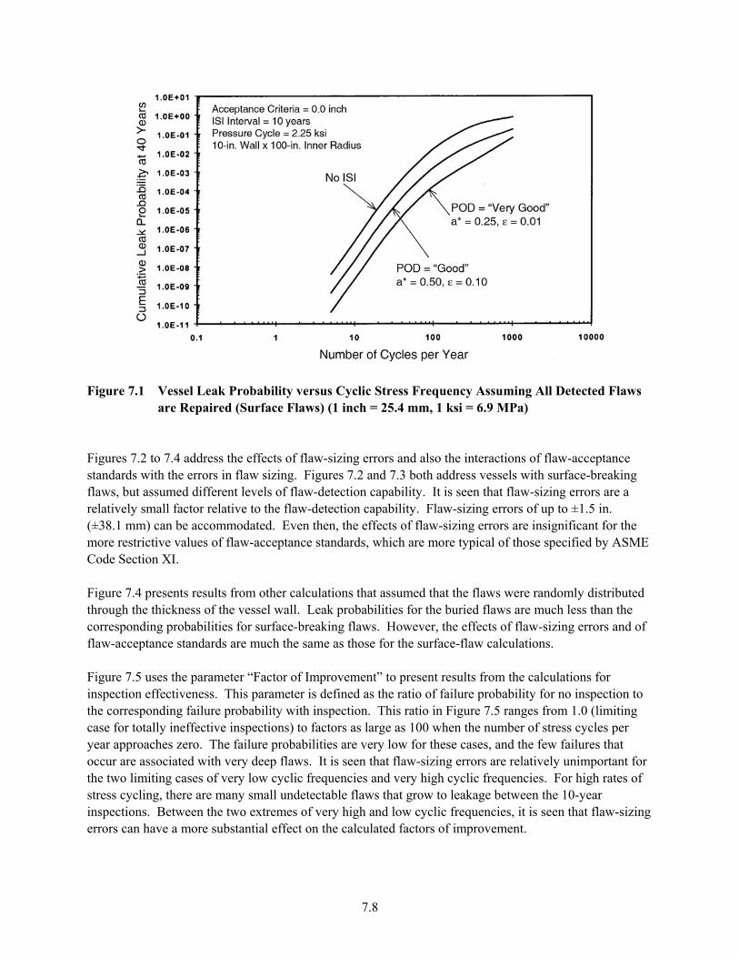
Figure 7.1 Vessel Leak Probability versus Cyclic Stress Frequency Assuming All Detected Fl
are Repaired (Surface Flaws) (1 inch = 25.4 mm, 1 ksi = 6.9 MPa)
aws
E
wever, the effects of flaw-sizing errors and of
ment” to present results from the calculations for n to
or these cases, and the few failures that t for s of
yclic frequencies, it is seen that flaw-sizing more substantial effect on the calculated factors of improvement.
Figures 7.2 to 7.4 address the effects of flaw-sizing errors and also the interactions of flaw-acceptance standards with the errors in flaw sizing. Figures 7.2 and 7.3 both address vessels with surface-breaking flaws, but assumed different levels of flaw-detection capability. It is seen that flaw-sizing errors are a
latively small factor relative to the flaw-detection capability. Flaw-sizing errors of up to ±1.5 in. re(±38.1 mm) can be accommodated. Even then, the effects of flaw-sizing errors are insignificant for themore restrictive values of flaw-acceptance standards, which are more typical of those specified by ASMCode Section XI. Figure 7.4 presents results from other calculations that assumed that the flaws were randomly distributedthrough the thickness of the vessel wall. Leak probabilities for the buried flaws are much less than the orresponding probabilities for surface-breaking flaws. Hoc
flaw-acceptance standards are much the same as those for the surface-flaw calculations.
igure 7.5 uses the parameter “Factor of ImproveFinspection effectiveness. This parameter is defined as the ratio of failure probability for no inspectiothe corresponding failure probability with inspection. This ratio in Figure 7.5 ranges from 1.0 (limiting case for totally ineffective inspections) to factors as large as 100 when the number of stress cycles per
ear approaches zero. The failure probabilities are very low fyoccur are associated with very deep flaws. It is seen that flaw-sizing errors are relatively unimportanthe two limiting cases of very low cyclic frequencies and very high cyclic frequencies. For high ratestress cycling, there are many small undetectable flaws that grow to leakage between the 10-year
spections. Between the two extremes of very high and low cinerrors can have a
7.8
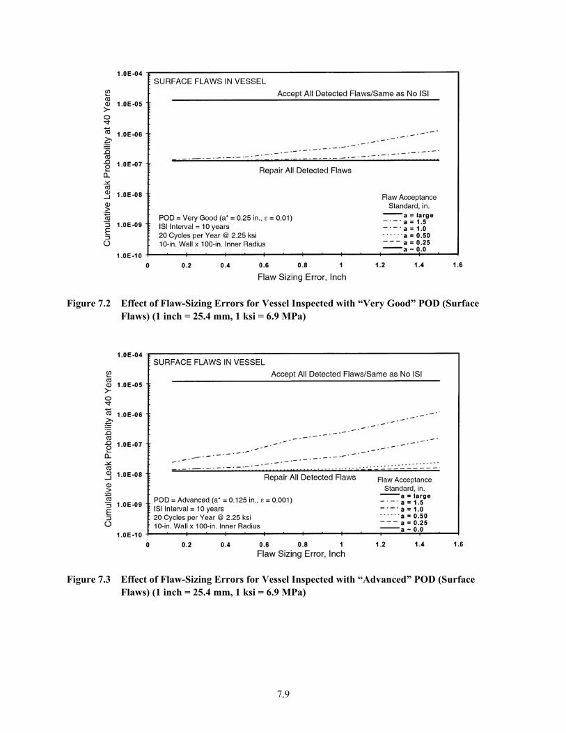
Figure 7.2 Effect of Flaw-Sizing Errors for Vessel Inspected with “Very Good” POD (Surface
Flaws) (1 inch = 25.4 mm, 1 ksi = 6.9 MPa)
Figure 7.3 Effect of Flaw-Sizing Errors for Vessel Inspected with “Advanced” POD (Surface
Flaws) (1 inch = 25.4 mm, 1 ksi = 6.9 MPa)
7.9

Figure 7.4 Effect of Flaw-Sizing Errors for Vessel Inspected with “Advanced” POD (Buried
Flaws) (1 inch = 25.4 mm, 1 ksi = 6.9 MPa)
Figure 7.5 Factor of Improvement for Vessel Inspected with “Very Good” POD (Surface Flaws
(1 inch = 25.4 mm, 1 ksi = 6.9 MPa) )
7.10
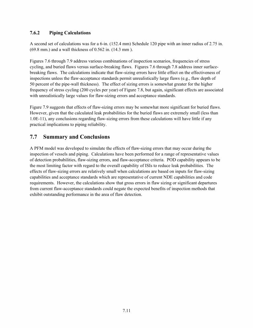
7.6.2 Piping Calculations
A second set of calculations was for a 6-in. (152.4 mm) Schedule 120 pipe with an inner radius of 2.75 in.
igures 7.6 through 7.9 address various combinations of inspection scenarios, frequencies of stress
s of ndards permit unrealistically large flaws (e.g., flaw depth of
0 percent of the pipe-wall thickness). The effect of sizing errors is somewhat greater for the higher
l (less than .0E-11), any conclusions regarding flaw-sizing errors from these calculations will have little if any
es eptance criteria. POD capability appears to be
e most limiting factor with regard to the overall capability of ISIs to reduce leak probabilities. The
tance standards could negate the expected benefits of inspection methods that
xhibit outstanding performance in the area of flaw detection.
(69.8 mm.) and a wall thickness of 0.562 in. (14.3 mm ). Fcycling, and buried flaws versus surface-breaking flaws. Figures 7.6 through 7.8 address inner surface-breaking flaws. The calculations indicate that flaw-sizing errors have little effect on the effectivenesinspections unless the flaw-acceptance sta5frequency of stress cycling (200 cycles per year) of Figure 7.8, but again, significant effects are associated with unrealistically large values for flaw-sizing errors and acceptance standards. Figure 7.9 suggests that effects of flaw-sizing errors may be somewhat more significant for buried flaws. However, given that the calculated leak probabilities for the buried flaws are extremely smal1practical implications to piping reliability. 7.7 Summary and Conclusions
A PFM model was developed to simulate the effects of flaw-sizing errors that may occur during the inspection of vessels and piping. Calculations have been performed for a range of representative valuof detection probabilities, flaw-sizing errors, and flaw-acctheffects of flaw-sizing errors are relatively small when calculations are based on inputs for flaw-sizing capabilities and acceptance standards which are representative of current NDE capabilities and code requirements. However, the calculations show that gross errors in flaw sizing or significant departuresfrom current flaw-accepe
7.11
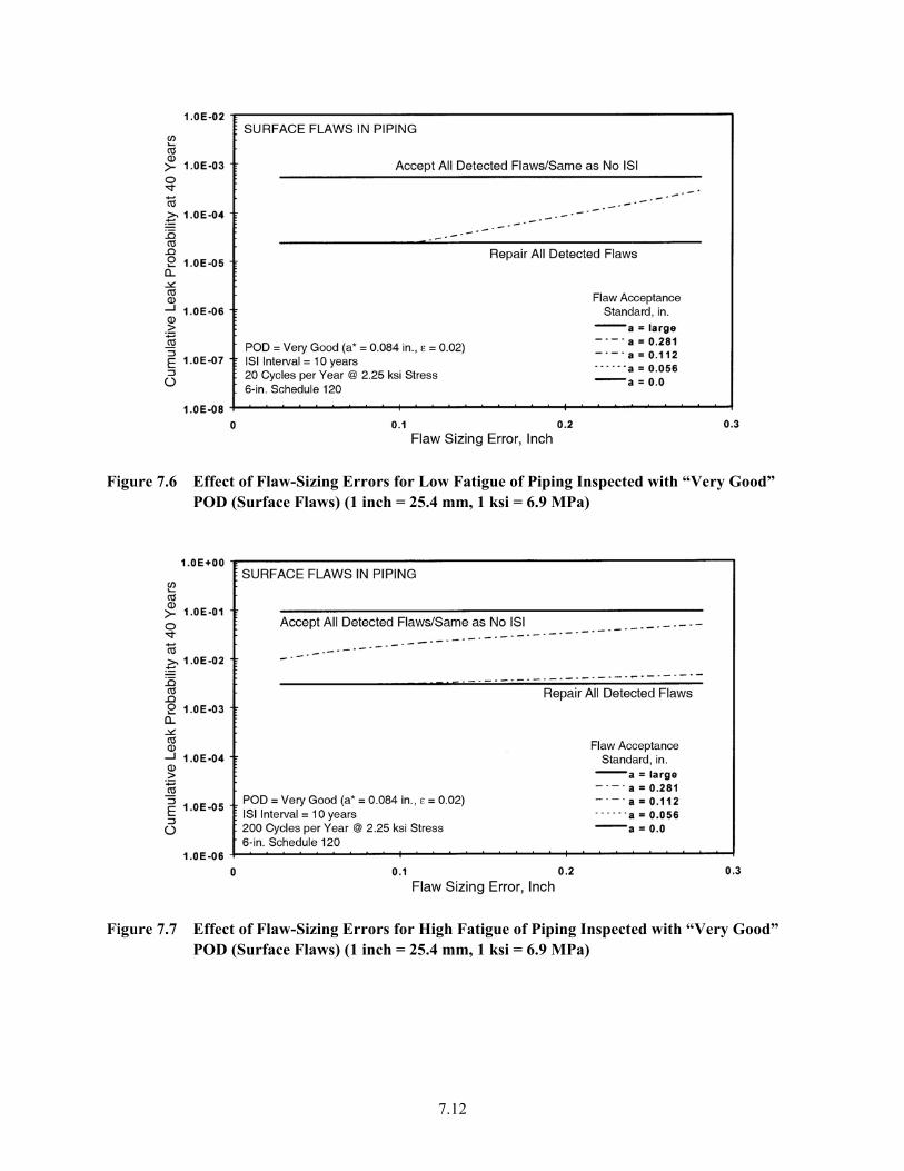
Figure 7.6 Effect of Flaw-Sizing Errors for Low Fatigue of Piping Inspected with “Very Good”
POD (Surface Flaws) (1 inch = 25.4 mm, 1 ksi = 6.9 MPa)
Figure 7.7 Effect of Flaw-Sizing Errors for High Fatigue of Piping Inspected with “Very Good”
POD (Surface Flaws) (1 inch = 25.4 mm, 1 ksi = 6.9 MPa)
7.12
Fig aw-Sizing Errors for High Fatigu of th “Advanced”
laws) (1 inch = 25.4 mm, 1 ks
ure 7.8 Effect of FlPOD (Surface F
e Piping Inspected wii = 6.9 MPa)
Fig law-Sizing Errors for Low Fatigue th “Very Good”
laws) (1 inch = 25.4 mm, 1 ksi = 6.9 MPa)
ure 7.9 Effect of FPOD (Buried F
of Piping Inspected wi
7.13

7.14
8.1
8 Conclusions
This report has described a large body of results that demonstrate the capabilities and benefits of probabilistic fracture mechanics calculations. This work has also shown many of the limitations and uncertainties associated with such calculations. Numerical results from the computational effort have supported both the U.S. Nuclear Regulatory Commission and the ASME Section XI Code in the development and implementation of risk-informed inservice inspection for operating nuclear power plants. Another application of the work is to support the development of improved non-destructive examination methods by relating improvements in piping and vessel reliability to improvement in NDE capabilities. Specific results and conclusions of the present report are: (1) A simulation model as described in Section 2 has been applied to estimate flaw densities and size
distributions for welds in piping systems. Calculations with the model addressed a range of pipe sizes, piping materials, welding methods, and inspection practices. Based on these calculations, recommendations were developed for inputs for the number and sizes of welding fabrication flaws to be used in probabilistic fracture mechanics simulations.
(2) The probabilistic fracture mechanics calculations as described in Section 3 were performed using a
structured parametric format in order to study the effects of important design and operating conditions on calculated piping failure probabilities for the damage mechanism of fatigue. Critical inputs included stresses from internal pressure, thermal expansion bending moments, through-wall thermal gradients, and low probability seismic and accident loadings. Other important inputs addressed pipe size, piping material, leak detection sensitivity, and inservice inspection programs as characterized by flaw detection probability and the periodic inspection frequency. The results of Section 3 can be applied to estimate piping failure frequencies without the need to perform detailed probabilistic fracture mechanics calculations.
(3) Additional fatigue calculations as described in Section 4 address stainless steel piping with a focus on
inservice inspection programs. The results quantify the benefits of alternative inspection programs that use ultrasonic examinations of welds. The calculations cover a wide range of probability of detection capabilities as well as inservice inspection frequencies. It is shown that high-quality inservice inspections can significantly reduce leak and break probabilities, particularly if the inspections are performed relatively frequently. Results of the probabilistic fracture mechanics calculations are presented as a collection of plots that can be used to select inspection strategies consistent with the goals of risk-informed inservice inspection programs.
(4) Probabilistic fracture mechanics calculations as described in Section 5 also address failure
probabilities for stainless steel piping but for the degradation mechanism of intergranular stress corrosion cracking. The fracture mechanics model accounts for material-related factors such as the degree of sensitization for weld locations. Other factors addressed by the model are related to operating conditions including residual stress, temperature, and environmental factors (e.g., oxygen level). Results of calculations are presented with a collection of plots that quantify reductions of failure probabilities as a function of NDE reliability (probability of detection curves) and inspection frequency. It is shown that significant reductions in failure probabilities require both a sensitive ultrasonic examination and a sufficiently small time interval between inspections.
8.2
(5) The calculations of Section 6 quantify the level of uncertainty associated with calculated failure probabilities for piping components. These evaluations supported the development of the methodology for risk-informed inservice inspection programs. The calculations show large uncertainties in calculated failure probabilities that are particularly large when the failure probabilities are very low such as for pipe rupture frequencies. The greatest source of uncertainty was indentified as inputs for initial density and size distributions for fabrication related flaws.
(6) A final set of calculations as presented in Section 7 address the effects of flaw sizing errors on the
reliability of vessels and piping systems. A probabilistic fracture mechanics model was developed to simulate the effects of flaw sizing errors along with both flaw detection capabilities and flaw-acceptance criteria. Inputs to the calculation were selected to represent current NDE capabilities and ASME Section XI Code flaw acceptance standards. The calculations showed that probability of detection is the most limiting factor with regard to the overall capability of an inservice inspection to reduce failure probabilities. The effects of flaw sizing errors are relatively small because of the conservative basis for flaw acceptance standards.
The scope of the present calculations was limited by the available computer codes for probabilistic fracture mechanics simulations. While the results of the calculations as presented in this report have wide-ranging applications, additional calculations can provide further benefits. Future advances in the capabilities of facture mechanics codes should permit more accurate calculations to be performed to address additional degradation mechanisms such as primary water stress corrosion cracking. Improve-ments are also expected in the capabilities of non-destructive examination methods and additional calculations will be useful to quantify the benefits of improved NDE expressed in terms of potential reductions in failure probabilities for vessel and piping components.
9.1
9 References
Andresen PL and FP Ford. 1994. “Fundamental Modeling of Environment Cracking for Improved Design and Lifetime Evaluation in BWRs.” Int J Pres Ves Pip 59(1–3):61–70. ASME/CRTD. 1992. Risk-Based Inspection - Development of Guidelines: Volume 2 - Part 1 Light Water Reactor (LWR) Nuclear Power Plant Components. CRTD-Vol. 20-2. Center for Research and Technology Development, American Society of Mechanical Engineers. Balkey KR, NB Closky and RK Perdue. 1997. “Identifying Structural Elements and Examination Requirements in a Risk-Informed Inservice Inspection Program for Piping.” In Risk-Informed Decision Making, PVP-Vol. 358, pp. 3–13. American Society of Mechanical Engineers, New York. Bates DJ, SR Doctor, PG Heasler and E Burck. 1987. Stainless Steel Round Robin Test: Centrifugally Cast Stainless Steel Screening Phase. NUREG/CR-4970, PNL-6266, PISC III Report No. 3. U.S. Nuclear Regulatory Commission, Washington, D.C. Becher PE and B Hansen. Undated. Statistical Evaluation of Defects in Welds and Design Implications. Danish Welding Institute, Danish Atomic Energy Commission, Research Establishments, RISO. Berens AP and PW Hovey. 1984. Flaw Detection Reliability Criteria, Vol. 1, Method and Results. AFWALTR844022. Air Force Wright Aeronautical Laboratories, Wright Patterson Air Force Base, Ohio. Bishop BA. 1997. “An Updated Structural Reliability Model for Piping Risk Informed ISI.” In Fatigue and Fracture - 1997, Volume 2, PVP Vol. 346, pp. 245–252. American Society of Mechanical Engineers, New York. Bozarth D, CL Mason and JW Minarick. 1985. “Sensitivity and Uncertainty Analyses of Estimated Through Wall Crack Frequencies for H.B. Robinson Unit 2.” In Pressurized Thermal Shock Evaluation of the H.B Robinson Unit 2 Nuclear Power Plant, Vol. 1. Ch. 7. U.S. Nuclear Regulatory Commission, Washington, D.C. Bruckner-Foit A, T Schmidt and J Theodoropoulos. 1989. “A Comparison of the PRAISE Code and the PARIS Code for the Evaluation of Failure Probability of Crack-Containing Components.” Nuclear Engineering and Design 110(3):395–411. Burns ET, DO Harris and RC Erdmann. 1978. Reliability of Nuclear Piping Systems with Consideration of Cases Where Design Points Have Been Exceeded. Report SAI-091-79-PA. Science Applications Inc., Palo Alto, California. Presented at ASME/CSME Pressure Vessels and Piping Conference, Montreal, Canada. Chang CM, IK Chen, HK Shee, HY Chen and JN Yang. 1994. “Xray Inspection Reliability for Welded Joints.” In Structural Safety and Reliability: Proceedings of ICOSSAR ‘93, 6th International Conference, 9-13 August 1993, pp. 991–996. Innsbruck, Austria. eds: GI Schueller, M Shinozuka and JTP Yao.
9.2
Chapman OJV. 1993. “Simulation of Defects in Weld Construction.” In Reliability and Risk in Pressure Vessels and Piping, PVP-Vol. 251, pp. 81–89. American Society of Mechanical Engineers, New York. Chapman OJV, MA Khaleel and FA Simonen. 1996. “A Simulation Model for Estimating Probabilities of Defects in Weld.” In Fatigue and Fracture - 1996 - Volume 1, PVP-Vol. 323, pp. 375–391. American Society of Mechanical Engineers, New York. Chapman OJV and FA Simonen. 1998. RR-PRODIGAL – A Model for Estimating the Probabilities of Defects in Reactor Pressure Vessel Welds. NUREG/CR-5505, PNNL-11898. U.S. Nuclear Regulatory Commission, Washington, D.C. Cowfer CD. 1989. “Basis/Background for ASME Code Section XI Proposed Appendix VIII: Ultrasonic Examination Performance Demonstration.” In ASME Conference Publication, NDE-Vol. 5, pp. 1–5. American Society of Mechanical Engineers, New York. Cramond Jr. R. 1974. A Probabilistic Analysis of Structural Reliability Against Fatigue and Failure. PhD Thesis, University of Illinois at Urbana, Champaign, Illinois. Dickson TL. 1994. FAVOR: A Fracture Mechanics Analysis Code for Nuclear Reactor Pressure Vessels, Release 9401. ORNL/NRC/LTR/94/1. Martin Marietta Energy Systems, Inc., Oak Ridge National Laboratory, Oak Ridge, Tennessee. Dickson TL, JA Keeney and JW Bryson. 1995. “Validation of FAVOR Code Linear Elastic Fracture Solutions for Finite-Length Flaw Geometries.” In Fatigue and Fracture Mechanics in Pressure Vessels and Piping, PVP-Vol. 304, pp. 51–60. American Society of Mechanical Engineers, New York. Doctor SR, FL Becker, PG Heasler and GP Selby. 1983. “Effectiveness of U.S. Inservice Inspection Technologies: A Round Robin Test.” In Proceedings of a Specialist Meeting on Defect Detection and Sizing, Vol. 2 (CSNI Report No. 75 and EUR 9066 II EN), pp. 669–678. EPRI. 1989. Accuracy of Ultrasonic Flaw Sizing Techniques for Reactor Pressure Vessels. NP-6273. Electric Power Research Institute, Palo Alto, California. Frost NE and K Denton. 1967. “The Fatigue Strength of Butt Welded Joints in Low Alloy Structural Steel.” British Welding Journal 14(4):156–161. General Electric Company. 1982a. The Growth and Stability of Stress Corrosion Cracks in Large Diameter BWR Piping, Volume 1: Summary. EPRI NP-2472, Vol. 1. BWR Owners Groups and Electric Power Research Institute, Palo Alto, California. General Electric Company. 1982b. The Growth and Stability of Stress Corrosion Cracks in Large Diameter BWR Piping, Volume 2: Appendixes. EPRI NP-2472, Vol. 2. BWR Owners Groups and Electric Power Research Institute, Palo Alto, California.
9.3
Goldberg A, RD Streit and RG Scott. 1980. Evaluation of Cracking in Feedwater Piping Adjacent to the Steam Generators in Nine Pressurized Water Reactor Plant. UCRL-53000, NUREG/CR-1603. Lawrence Livermore National Laboratory, Livermore, California. Halmshaw R and CA Hunt. 1975. “Can Cracks Be Found by Radiography?” Brit J Nondestr Test May, pp. 71–75. Harris DO. 1977. “Relative Rupture Probabilities at Various Locations in Reactor Coolant Piping.” T Am Nucl Soc 26:404. Harris DO. 1978. “Probabilistic Analysis of Rupture in Reactor Coolant Piping.” In Proceedings of Topical Meeting, Probabilistic Analysis of Nuclear Reactor Safety, Vol. 2, Paper II.7. American Nuclear Society, Los Angeles, California. Harris DO. 1981. “Stress Corrosion Crack Growth in the Presence of Residual Stresses.” In Proceedings of the 28th Sagamore Army Materials Research Conference, Lake Placid, New York. Harris DO and DD Dedhia. 1992. A Probabilistic Fracture Mechanics Code for Piping Reliability Analysis (pc-PRAISE Code). NUREG/CR-6237. U.S. Nuclear Regulatory Commission, Washington, D.C. Harris DO, DD Dedhia and ED Eason. 1986a. “Probabilistic Analysis of Initiation and Growth of Stress Corrosion Cracks in BWR Piping.” American Society of Mechanical Engineers, New York. ASME Paper 86-PVP-11. Harris DO, DD Dedhia, ED Eason and SD Patterson. 1986b. Probability of Failure in BWR Reactor Coolant Piping: Probabilistic Treatment of Stress Corrosion Cracking in 304 and 316NG BWR Piping Weldments. NUREG/CR-4792, Vol. 3. U.S. Nuclear Regulatory Commission, Washington, D.C. Harris DO, DD Dedhia and SC Lu. 1992. Theoretical and User’s Manual for pc-PRAISE, A Probabilistic Fracture Mechanics Computer Code for Piping Reliability Analysis. NUREG/CR-5864. U.S. Nuclear Regulatory Commission, Washington, D.C. Harris DO and RR Fullwood. 1976. An Analysis of the Relative Probability of Pipe Rupture at Various Locations in the Primary Cooling Loop of a Pressurized Water Reactor Including the Effects of a Periodic Inspection. Report SAI-001-PA. Science Applications, Inc., Palo Alto, California. Harris DO and EY Lim. 1983. “Application of a Probabilistic Fracture Mechanics Model to the Influence of In-Service Inspection on Structure Reliability.” In Probabilistic Fracture Mechanics and Fatigue Methods: Applications for Structural Design and Maintenance. eds: JM Bloom and JC Ekrall. American Society for Testing and Materials, West Conshohocken, Pennsylvania. STP 798. pp. 19–41. Harris DO, EY Lim and DD Dedhia. 1981. Probability of Pipe Fracture in the Primary Coolant Loop of a PWR Plant Volume 5: Probabilistic Fracture Mechanics Analysis - Load Combination Program Project 1 Final Report. NUREG/CR-2189, Vol. 5. U.S. Nuclear Regulatory Commission, Washington, D.C.
9.4
Hazelton W and WH Koo. 1988. Technical Report on Material Selection and Processing Guidelines for BWR Coolant Pressure Boundary Piping. NUREG-0313, Rev. 2. U.S. Nuclear Regulatory Commission, Washington, D.C. Heasler PG and SR Doctor. 1996. Piping Inspection Round Robin. NUREG/CR-5068, PNNL-10475. U.S. Nuclear Regulatory Commission, Washington, D.C. Heasler PG, TT Taylor, JC Spanner, SR Doctor and JD Deffenbaugh. 1990. Ultrasonic Inspection Reliability for Intergranular Stress Corrosion Cracks: A Round Robin Study of the Effects of Personnel, Procedures, Equipment and Crack Characteristics. NUREG/CR-4908, PNL-6179. U.S. Nuclear Regulatory Commission, Washington, D.C. Khaleel MA, OJV Chapman, DO Harris and FA Simonen. 1999. “Flaw Size Distribution and Flaw Existence Frequencies in Nuclear Piping.” In Probabilistic and Environmental Aspects of Fracture and Fatigue, PVP-Vol. 386, pp. 127–144. American Society of Mechanical Engineers, New York. Khaleel MA and FA Simonen. 1994a. “The Effects of Initial Flaw Sizes and Inservice Inspection on Piping Reliability.” In Service Experience and Reliability Improvement: Nuclear, Fossil, and Petrochemical Plants, PVP-Vol. 288, pp. 95–07. American Society of Mechanical Engineers, New York. Khaleel MA and FA Simonen. 1994b. “A Parametric Approach to Predicting the Effects of Fatigue on Piping Reliability.” In Service Experience and Reliability Improvement: Nuclear, Fossil, and Petrochemical Plants, PVP-Vol. 288, pp. 117–125. American Society of Mechanical Engineers, New York. Khaleel MA and FA Simonen. 1995. “A Model for Predicting Vessel Failure Probabilities Due to Fatigue Crack Growth.” In Fatigue and Fracture Mechanics in Pressure Vessels and Piping, PVP-Vol. 304, pp. 401–416. American Society of Mechanical Engineers, New York. Khaleel MA and FA Simonen. 1997. “Reliability-Based Inspection Planning for Stainless Steel Piping Under Conditions of Intergranular Stress Corrosion Cracking.” In Proceedings of ICOSSAR ‘97 - International Conference on Structural Safety and Reliability, November 24–28, 1997, Kyoto, Japan. Khaleel MA and FA Simonen. 1998. “A Probabilistic Model for Fatigue Crack Initiation and Propagation.” In Fatigue, Fracture and Residual Stresses, PVP-373, pp. 27–34. American Society of Mechanical Engineers, New York. Khaleel MA, FA Simonen, DO Harris and DD Dedhia. 1995. “The Impact of Inspection on Intergranular Stress Corrosion Cracking for Stainless Steel Piping.” In Risk and Safety Assessments: Where Is the Balance?, PVP-Vol. 296, pp. 411–422. American Society of Mechanical Engineers, New York. Marshall Committee. 1976. An Assessment of the Integrity of PWR Pressure Vessels. Report by a Study Group Chaired by Dr. W. Marshall, available from H.M. Stationary Office, London, October 1976.
9.5
Marshall Committee. 1982. An Assessment of the Integrity of PWR Pressure Vessel. Second Report by a Study Group under the Chairmanship of Dr. W. Marshall, published by the UKAEA. Nichols RW and S Crutzen, Eds. 1988. Ultrasonic Inspection of Heavy Section Steel Components: The PISC-II Final Report. Elsevier Applied Science Publishers, London and New York. Packman PF, SJ Kilma, RL Davies, J Malpani, J Moyzis, W Walker, BGW Yee and DP Johnson. 1976. “Reliability of Flaw Detection by Nondestructive Inspection.” In ASM Metals Handbook, Vol. 11, 8th Ed., Metals Park, Ohio. pp. 214–224. Parry GW. 1997. “Quality of PRA for Use in Regulatory Decision Making.” In Risk Informed Decision Making, PVP-Vol. 358, pp. 81–85. American Society of Mechanical Engineers, New York. Paul DD, N Ghadiali, J Ahmad and G Wilkowski. 1991. SQUIRT: Seepage Quantification of Upsets in Reactor Tubes. International Piping Integrity Research Group, Battelle, Columbus, Ohio. Phillips JH, WS Roesener, HL Magleby, WG Reuter and V Geidel. 1991. Development and Demonstration of Methods to Include Aging of Passive Components in RAs. NUREG/CR-5730. U.S. Nuclear Regulatory Commission, Washington, D.C. Shah NJ, DM Bucheit, A McNeill and EW Throckmorton. 1997. “Implementation of a Risk-Informed ISI Program at Surry Power Station.” In Risk-Formed Decision Making, PVP-Vol. 358, pp. 25–30. American Society of Mechanical Engineers, New York. Simonen FA. 1990. “An Evaluation of the Impact of Inservice Inspection on Stress Corrosion Cracking of BWR Piping.” In Codes and Standards and Applications for Design and Analysis of Pressure Vessel and Piping Components, PVP-Vol. 186, NDE-Vol. 7, pp. 187–193. American Society of Mechanical Engineers, New York. Simonen FA and OJV Chapman. 1999. “Measured Versus Predicted Distributions of Flaws for Piping Welds.” In Probabilistic and Environmental Aspects of Fracture and Fatigue, PVP-Vol. 386, pp. 101–103. August 1–5, 1999, Boston, Massachusetts. American Society of Mechanical Engineers, New York. Simonen FA, DO Harris and DD Dedhia. 1998. “Effect of Leak Detection on Piping Failure Probabilities.” In Fatigue Fracture and Residual Stress, PVP-Vol. 373, pp. 105–113. American Society of Mechanical Engineers, New York. Simonen FA, KI Johnson, AM Liebetrau, DW Engel and EP Simonen. 1986. VISA-II - A Computer Code for Predicting the Probability of Reactor Pressure Vessel Failure. NUREG/CR-4486. U.S. Nuclear Regulatory Commission, Washington, D.C. Simonen FA and MA Khaleel. 1997. “Effects of Flaw Sizing Errors on the Reliability of Vessels and Piping.” In Fatigue and Fracture, 1997, PVP-Vol. 346, pp. 233–243. American Society of Mechanical Engineers, New York.
9.6
Simonen FA and MA Khaleel. 1998a. “On the Contribution of Buried Flaws to Piping Failure Probabilities.” In Fatigue Fracture and Residual Stress, PVP-Vol. 373, pp. 69–75. American Society of Mechanical Engineers, New York. Simonen FA and MA Khaleel. 1998b. “Uncertainty Analysis of Probabilistic Fracture Mechanics Calculations of Piping Failure Probabilities.” In Proceeding of the 4th International Conference on Probabilistic Safety Assessment and Management, Probabilistic Safety Assessment and Management PSAM 4, Vol. 3, pp. 2040–2045. September 13–18, 1998, New York. Simonen FA and HH Woo. 1984. Analyses of the Impact of Inservice Inspection Using a Piping Reliability Model. NUREG/CR-3869. U.S. Nuclear Regulatory Commission, Washington, D.C. Taylor TT, JC Spanner, PG Heasler, SR Doctor and JD Deffenbaugh. 1989. “An Evaluation of Human Reliability in Ultrasonic Inservice Inspection for Intergranular Stress Corrosion Cracking Through Round Robin Testing.” Mater Eval 47:338. Thomas HM. 1979. “In-Service Inspection is Overrated.” J Inst Mech Eng 20(2):43–56. USNRC. 1997. An Approach for Plant-Specific, Risk-Informed Decisionmaking: Inservice Inspection of Piping. Draft Regulatory Guide DG-1063. U.S. Nuclear Regulatory Commission, Washington, D.C. Westinghouse Owners Group. 1997. Application of Risk-Informed Methods to Piping Inservice Inspection Topical Report. WCAP-14572, Rev. 1. Westinghouse Electric Co., Pittsburgh, Pennsylvania. Wilkowski G, G Kramer, P Veith, R Francini and P Scott. 1994. “The Effect of Dynamic and Cyclic Loading During Ductile Tearing on Circumferentially Cracked Pipe: Analytical Results.” In Fatigue, Flaw Evaluation and Leak Before Break Assessments, PVP-Vol. 280, pp. 221–239. American Society of Mechanical Engineers, New York. Wilson AS. 1974. Estimating the Relative Probability of Pipe Severance by Fault Cause. GEAP-20615. General Electric Company, San Jose, California. Woo HH and CH Chou. 1982. Piping Reliability Model Validation and Potential Use for Licensing Regulation Development. NUREG/CR-2801. U.S. Nuclear Regulatory Commission, Washington, D.C. Woo HH and FA Simonen. 1984. “The Impact of Inservice Inspection on the Reliability of Nuclear Piping.” In Advances in Probabilistic Fracture Mechanics, PVP-Vol. 92. American Society of Mechanical Engineers, New York.
NUREG/CR-XXXX PNNL-13810
Distribution No. of No. of Copies Copies
Distr.1
Nuclear Regulatory Commission TL Chan
NRC/NRR Mail Stop O-9 H6
SC Dinsmore NRC/NRR Mail Stop O-10 C15
BJ Elliot
NRC/NRR Mail Stop O-9 H3
RO Hardies
NRC/RES Mail Stop T-10 E10
MT Kirk
NRC/RES Mail Stop T-10 E10
SNM Malik
NRC/RES Mail Stop T-10 E10
KA Manoly
NRC/NRR Mail Stop O-9 D3
MA Mitchell
NRC/NRR Mail Stop O-9 H6
D Naujock
NRC/NRR Mail Stop O-9 H6
WE Norris
NRC/RES Mail Stop T-10 E10
CA Nove
NRC/NRR Mail Stop O-9 H6
IG Prokofiev NRC/RES Mail Stop T-10 M5
TJ Sullivan Jr.
NRC/NRR Mail Stop O-9 H6
D Terao
NRC/NRO Mail Stop T-7 F1
RL Tregoning
NRC/RES Mail Stop T-10 M5
JL Uhle
NRC/RES Mail Stop T-10 M5
Offsite BR Bass Oak Ridge National Laboratory MS 6085 PO Box 2008 Oak Ridge, TN 37831 BA Bishop Westinghouse Nuclear Services P.O. Box 158 (Bin 18) or
Exit 54 Interstate 70 Madison, PA 15663 TL Dickson Oak Ridge National Laboratory MS 6085 PO Box 2008 Oak Ridge, TN 37831 R. Gamble Sartrex Corporation 1700 Rockville Pike, Suite 400 Rockville, MD 20852
No. of No. of Copies Copies
Distr.2
DO Harris Structural Integrity Associates, Inc. 3315 Almaden Expressway Suite 24 San Jose, CA 95118 ST Rosinski EPRI NDE Center 1300 Harris Blvd. Charlotte, NC 28262 DL Rudland Engineering Mechanics Corporation of
Columbus 3518 Riverside, Dr., Suite 202 Columbus, OH 43220 PM Scott Battelle Columbus 505 King Avenue Columbus, OH 43201 GP Selby EPRI NDE Center 1300 Harris Blvd. Charlotte, NC 28262 JC Spanner, Jr. EPRI NDE Center 1300 Harris Blvd. Charlotte, NC 28262
GM Wilkowski Engineering Mechanics Corporation of
Columbus 3518 Riverside, Dr., Suite 202 Columbus, OH 43220 PT Williams Oak Ridge National Laboratory MS 6085 PO Box 2008 Oak Ridge, TN 37831 40 Internal Distribution
Pacific Northwest National Laboratory P.O. Box 999 Richland, WA 99352 MT Anderson (28) K5-25 A Ankrum K6-66 SE Cumblidge K5-25 AA Diaz K5-25 SR Doctor K5-25 PG Heasler K6-08 M Khaleel K9-80 AF Pardini K5-25 FA Simonen (4) K5-22 TT Taylor K5-25 Information Release PDF


