This joint research programme was initiated by ERA-NET ROAD. EVITA Environmental Indicators for the Total Road Infrastructure Assets Effective asset management meeting future challenges Cross-border funded Joint Research Programme by Belgium (Flanders), Denmark, Finland, France, Germany, Ireland, Lithuania, Netherlands, Norway, Slovenia, Sweden, Switzerland, and United Kingdom. Deliverable D3.1 Report on recommended E-KPIs Revised version - August 2012
Transcript
This joint research programme was initiated by ERA-NET ROAD.
EVITA Environmental Indicators for the Total Road Infrastructure Assets
Effective asset management meeting future challenges Cross-border funded Joint Research Programme by Belgium (Flanders), Denmark, Finland, France, Germany, Ireland, Lithuania, Netherlands, Norway, Slovenia, Sweden, Switzerland, and United Kingdom. Deliverable D3.1
Report on recommended E-KPIs Revised version - August 2012
ENR SRO4 AF initiated by
Page 2 of 58
Deliverable D3.1
CONTRACT No : 09/16771-40 ACRONYM: EVITA
TITLE: Environmental Indicators for the Total Road Infrastructure Assets
PROJECT COORDINATORS: Institut Français des Sciences et des Technologies des Transports, de l’Aménagement et des Réseaux (F) PMS-Consult (AT)
OTHER PARTNERS :
Laboratório Nacional de Engenharia Civil (LNEC) P Transport Research Laboratory (TRL) UK Zavod za gradbenistvo Slovenije - Slovenian National Building & Civil Engineering Institute (ZAG)
SI
DRI Investment Management, Company for Development of Infrastructure Ltd. SI University of Belgrade, Faculty of Civil Engineering SR
Report coordinated by: Marcus Jones
Contributors: Trevor Bradbury Julien Cesbron
Ben Harris Darko Kokot Alaric Lester
Craig Thomas Helen Viner
Alfred Weninger-Vycudil
Reviewed by: Vijay Ramdas
Reviewed by:
J.Litzka
Date of issue of this report : Revised August 2012
Project funded by the ERAnet Road 2 Programme (2010 - 2013)
ENR SRO4 AF initiated by
Page 3 of 58
EVITA
Environmental Indicators for the Total Road Infrastructure Assets
Abstract Glossary
The following words are frequently used in the EVITA reports. An attempt of definition in this context is proposed below. Road Infrastructure / road asset: All constructions (pavements, bridges, drainage structures…) and equipment (safety barriers, signs, lights…), including the land reservation which composed the facilities devoted to road transport. Road asset management: All studies, decision makings and operations which are specifically aiming at or required to build, maintain and operate the road infrastructure/road asset. Road Stakeholder: All people (physical or social person), all organisations, and more generally all bodies, which have some interactions with road infrastructure. The road network can provide benefits to stakeholders as well as imposing constraints upon them. Conversely, the needs of stakeholders may also impose constraints on, or determine the requirements of, the infrastructure. Expectation: Anything that a stakeholder is requiring from the road infrastructure. It may be some services, some benefits, or it may be the reduction of some nuisances. Road performance: Generally, the ability of the road to answer expectations, to provide a stakeholder with what he is expecting from the road. More specifically, road performance is a measure of this ability to meet expectations, of the quality of the road regarding the expected service or characteristics or impacts. Performance Indicator: A comprehensive term which quantifies the road performance. It can be expressed in the form of a technical parameter (dimensional) and/or finally in form of an index (dimensionless) evaluating the performance indicator on a predefined scale
- KPI ……..Key performance indicator for a given characteristic or parameter - E-KPI ……Key performance indicator related to environmental aspects
ENR SRO4 AF initiated by
Page 4 of 58
Single Performance Indicator: A dimensional or dimensionless number related to only one technical characteristic of the road pavement, indicating the condition of that characteristic (for example: noise) (also called Individual Performance Indicator). Combined Performance Indicator: A dimensional or dimensionless number related to two or more different characteristics of the road pavement, that indicates the condition of all the characteristics involved (for example, noise and air pollution). Performance Index: An assessed Technical Parameter of the road pavement, dimensionless number or letter on a scale that evaluates the Technical Parameter involved (e.g. Noise, GHG, etc.) on a 0 to 5 scale, 0 being a very good condition and 5 a very poor one. Technical Parameter (TP): A physical characteristic of the road pavement condition, derived from various measurements, or collected by other forms of investigation (for example, noise level). Transfer Function: A mathematical function used to transform a technical parameter into a dimensionless performance index.
ENR SRO4 AF initiated by
Page 5 of 58
EVITA
Environmental Indicators for the Total Road Infrastructure Assets Deliverable D 3.1
Executive summary The main objective of the project “EVITA – Environmental Performance Indicators for the Total Road Infrastructure Assets” is the development and integration of new and existing key performance indicators in the asset management process taking into account the expectations of different stakeholders (users, operators, neighbours, etc.). A priority for the project is the development of Environmental KPIs (E-KPIs) that are easy to understand and use. This deliverable is a report on the third Work Package (WP 3) of the project. This WP was devoted to the development of the environmental indicators identified in the previous WPs, under the following headings:
- noise - air pollution (including emissions of CO2 from vehicles) - water pollution - natural resources (including lifecycle CO2 emissions arising from construction and
maintenance activities) Each E-KPI will use different input variables in form of Technical Parameter(s) or Single Performance Indice(s). To provide a consistent basis for quantitative analysis, each E-KPI will be expressed as a dimensionless index on a scale from 0 (good condition) to 5 (poor condition), using appropriate transformation functions. Summary of indicators chosen. Noise impacts A three level indicator has been developed:
• Emission indicator based on physical measurements of noise level • Exposure indicator based on noise exposure and thresholds • Impact indicator based on noise exposure and ‘annoyance’
Air quality impacts of vehicle emissions Two categories of indicator are proposed:
• An emissions rate indicator for each of NOx and PM based upon total modelled emissions using traffic data and vehicle emission factors; and
• An exposure indicator for each of NO2 and PM10, reflecting their health impacts, based upon an assessment of the exposed population to concentrations above EU limit values.
CO2 emissions from vehicles As CO2 only has an impact at a global level, the impact of a scheme is determined by its effect on total CO2 emissions and hence its impact on carbon reduction targets. An emissions based indicator only is proposed, using modelled emissions from traffic flows and vehicle emission factors.
ENR SRO4 AF initiated by
Page 6 of 58
Water quality Standards for water quality are based upon measurements of the concentration of individual pollutants. However, obtaining sufficiently detailed data for individual schemes would be very costly and has the difficulty that there are many other sources of water pollution affecting water courses, making it harder to link the results directly to an individual scheme. The indicator proposed uses information more readily available to the road operator and more directly linked to factors within its control: 1. the total amount of pollutants generated (using data on the volume and type of traffic and level of road salt application); 2. the quality of the drainage system and any associated pollution control measures; and 3. the sensitivity of the local environment and ability of receiving watercourses to dilute and disperse any contaminants. Two indicators are proposed:
• Water quality, based upon an assessment of pollution loadings, the sensitivity of the environment and the quality of the drainage systems; and
• Salt, based upon a comparison of salt loadings for the road section being assessed against the average for the network, weighted by local requirements and the sensitivity of the environment.
Natural resources Impacts are linked to the extraction of virgin material, the energy and other impacts of production and construction processes, disposal of waste, and impacts of transporting it to and from the site. Care is needed in the development of indicators to avoid perverse outcomes, for example promoting the unreasonably long-distance transport of recycled material when new aggregate is available locally, so the indicator needs to take full account of life-cycle impacts. Two indicators are proposed for use when the user has all the necessary data available:
• Material Resource Efficiency Indicator (MREI): recycled content of construction material weighted to represent the relative impact on natural resources as a proportion of overall materials used; and
• Embodied Carbon Reduction Indicator (ECRI): the reduction in Carbon Dioxide emissions for a maintenance strategy against a nominal strategy that would demonstrate the maximum emissions of carbon dioxide.
Two alternative approaches to calculating MREI are also identified. These approaches can be used where data is more limited or a less complex calculation is desired. A simpler carbon assessment method is also included, Carbon Dioxide Reuse Potential (CaRP). This is a useful tool for monitoring performance but cannot as readily be converted to a dimensionless indicator as is the case for the preferred carbon indicator.
ENR SRO4 AF initiated by
Page 7 of 58
EVITA Environmental Indicators for the Total Road Infrastructure Assets
Table of contents Deliverable D 3.1 I - Introduction _____________________________________________________________ 8
I.1 The EVITA Project __________________________________________________________ 8
I.2 The Work Package 3 _________________________________________________________ 8
I.3 Background to the selected E-KPIs _____________________________________________ 9
I.4 The KPI framework_________________________________________________________ 10
I.5 Presentation of the E-KPIs ___________________________________________________ 11
II Proposed E-KPI for Noise _________________________________________________ 11
II.I Introduction to noise E-KPI _________________________________________________ 11
II.2 Basis for new noise E-KPIs __________________________________________________ 12
II.3 Methodology for noise E-KPIs _______________________________________________ 13
II.4 Worked example of application of noise E-KPI _________________________________ 17
II.5 Summary of noise E-KPIs ___________________________________________________ 19
III Proposed E-KPI for air quality and CO2 emissions from vehicles _________________ 20
III.1 Introduction to air quality and CO2 E-KPI ____________________________________ 20
III.2 Basis of air quality and CO2 E-KPI __________________________________________ 20
III.3 Methodology for air quality and CO2 E-KPI ___________________________________ 21
III.4 Worked example __________________________________________________________ 26
III.5 Summary of air quality and CO2 E-KPI ______________________________________ 28
IV Proposed E-KPI for water quality and the drainage system ______________________ 29
IV.1 Introduction to the water quality and drainage System E-KPI ____________________ 29
IV.2 Basis of the water quality and drainage system E-KPI ___________________________ 29
IV.3 Methodology for water pollution and drainage system E-KPI _____________________ 31
IV.4 Indicator for water pollution from winter maintenance (use of salt) ________________ 39
IV.5 Worked example __________________________________________________________ 41
IV.6 Summary of E-KPI for water quality and drainage system _______________________ 44
V Proposed E-KPI for natural resources _______________________________________ 45
V.1 Introduction to E-KPI for natural resources ____________________________________ 45
V.2 Basis of E-KPI for natural resources __________________________________________ 45
V.3 Methodology for Natural Resources E-KPI _____________________________________ 47
V.4 Worked example ___________________________________________________________ 54
V.5 Summary of natural resources E-KPI _________________________________________ 56
VI - References ____________________________________________________________ 57
ENR SRO4 AF initiated by
Page 8 of 58
EVITA
Environmental Indicators for the Total Road Infrastructure Assets
I - Introduction
I.1 The EVITA Project The main objective of the project “EVITA – Environmental Performance Indicators for the Total Road Infrastructure Assets” is the development and integration of new and existing environmental key performance indicators in the asset management process taking into account the expectations of different stakeholders (users, operators, neighbours, etc.). A priority for the project is the development of Environmental KPIs (E-KPIs) that are easy to understand and use. The project aims to identify existing best practice in the implementation of E-KPIs to managing the full range of road infrastructure components, (pavements, structures, road furniture, etc.). As described in previous project reports (D2.1 and D2.2) the project conducted a comprehensive state of the art investigation in cooperation with the client (through the PEB), with European Road Administrations and with other important road stakeholders such as Environment Agencies. In a second step, recommendations of different E-KPIs for the environmental areas “noise”, “air”, “water” and “natural resources” are given. Greenhouse gases, GHG, are considered both as emissions from vehicles in the “air” indicator and in terms of life cycle CO2 emissions within the “natural resources” indicator. Beside the definition of E-KPIs for these four main categories, a recommendation for the implementation and the use of E-KPIs will be included in this project as well, as reported in D4.1. This report presents the outcome of the third Work Package, which builds on the review and consultation stages to develop the proposed E-KPIs.
I.2 The Work Package 3 This WP was devoted to the development of the environmental indicators identified in the previous WPs, under the following headings:
- noise; - air pollution (including emissions of CO2 from vehicles); - water pollution; and - natural resources (including lifecycle CO2 emissions arising from construction and
maintenance activities). WP3 draws upon the review of existing KPIs and consultation with stakeholders that is reported in D2.1 and D2.2.
ENR SRO4 AF initiated by
Page 9 of 58
I.3 Background to the selected E-KPIs Following the review of E-KPIs undertaken in WP2 it was agreed that the E-KPIs taken forward for development in WP3 would be noise (N), air pollution (A), water pollution (W) and natural resources (R). a) Noise Noise emissions mainly affect those living near the road. The E-KPIs developed by WP3 will be based on noise mapping, using data both from sound-level measurements and modelling. If possible, the theoretical modelling used for noise mapping should be verified through in-situ measurements. b) Air pollution and greenhouse gas emissions Air pollution can be generated by traffic itself, during the whole life-cycle of the infrastructure, or by construction and maintenance activities, which take place at specific points in time. The most significant issues related to air pollution will be NOx and Particulate Matter (most usually measured as PM10 and PM2.5). The impacts of air pollution are usually greatest near to the road, however there is significant long range transport of air pollutants and many secondary pollutants, such as NO2 and ozone, form at considerable distance from the source and are therefore regional rather than local in impact. As CO2 only has an impact at a global level, the impact of a scheme is determined by its effect on total CO2 emissions. Other Greenhouse Gas emissions can be expressed as CO2
equivalent. It was agreed that CO2 emissions from traffic would be included as part of the air pollution indicators. c) Water pollution Water pollution due to road infrastructure is mainly attributed to wash-off pollutants from the surface of the road and can be mitigated through protective measures associated with the drainage system. Standards for water quality are based upon measurements of the concentration of individual pollutants. However, obtaining sufficiently detailed data for individual schemes would be very costly and has the difficulty that there are many other sources of water pollution affecting water courses, making it harder to link the results directly to an individual scheme. Indicators can be developed as a function of the quality of the drainage system and any pollution control measures associated with it. It is also necessary to take account of the extent of production of pollutants by the road traffic, and activities such as road salting, and the sensitivity of the environment into which run-off is discharged. d) Natural resources Depreciation of natural resources in road infrastructure is mainly associated with material and energy consumption as well as waste generated during construction and maintenance. It can be considered as a global problem that affects society in general, but it is also an issue for road owners, who are responsible for these activities. Impacts are linked to the extraction of virgin material, the energy and other impacts of production and construction processes, disposal of waste, and impacts of transporting it to and from the site. Care is needed in the development of indicators to avoid perverse outcomes, for example promoting the unreasonably long distance transport of recycled material when new aggregate is available locally, so the indicator needs to take full account of life-cycle impacts.
ENR SRO4 AF initiated by
Page 10 of 58
A summary of the indicators and their intended purpose
Domain Source Mitigation Impact Expectancies
Noise o Rolling noise o Motor noise
o Noise Walls o Wearing course o Traffic management
o Exposed population
o Annoyed population
o Reducing noise annoyance
Air quality o Emissions from
vehicles using road
o Low emission vehicle technology
o Traffic management measures (speed, flow)
o Demand management (reduce total amount of traffic)
o Health impacts on exposed populations
o Impacts on buildings
o Reducing total emissions
o Reducing numbers of exposed population
CO2 emissions from vehicles
o Emissions from vehicles using road
o Low carbon fuels and vehicles
o Traffic management o Demand management
o Climate change o Reducing total emissions
Water
o Water pollution by traffic (from exhaust, brake and engine wear, oil and fuel leaks)
o Water salted by WM (winter maintenance)
o Chemical spills from accidents
o Drainage system including water treatments
o Quantities of salt o Traffic management o Management of
hazardous loads
Pollution affecting water courses, ground water and land
o Hydrocarbon o Salt o Heavy metal
o Reducing pollution
Resources
o Consumption of non-renewable materials
o Energy consumption, CO2 emission, to produce material and construct infrastructures
o Apply the waste reduction hierarchy: ‘reduce’, ‘reuse’, ‘recycle’
o Consumption of non-renewable resources
o Consumption of energy
o Emission of CO2 or equivalent.
o Reduced use of mineral resources
o Reducing fossil energy consumption
o Reducing GHG emission
I.4 The KPI framework The framework and process for the implementation of the E-KPIs is developed in WP4 and described in detail in D4.1. A summarised description is therefore given here. Given the fact that, for many road networks, the available information on technical parameters related to the environment is still limited, the strategy for implementation/incorporation of E-KPIs should consider a minimum of information for development of simple, easily understandable, indicators that can be complemented with more sophisticated information for better accuracy. Each E-KPI will use different input variables in form of a Technical Parameter(s) or Single Performance Indicator(s). To provide a consistent basis for quantitative analysis, each E-KPI will be expressed as a dimensionless index on a scale from 0 (good condition) to 5 (poor condition), using appropriate transformation functions. The proposed process for developing a transformation from technical parameter (TP) to a dimensionless index (PI) is the one developed within COST 354 [1] and built upon by COST
ENR SRO4 AF initiated by
Page 11 of 58
356 [2] which consists of four steps, briefly described below. See also COST350 [3] for additional background information. 1. Decide on TP values with corresponding Index values (PI). It is necessary to define at least two values for the Technical Parameter with corresponding Index values. These points can be at any point in the Index scale. 2. Plot points on graph. This allows the relationship between the Technical Parameter and the Index to be seen. 3. Determine the line/curve of best fit. Choose a graph which best fits the points you have chosen, most likely to be a simple straight line fit. 4. Calculate and check the range and sensitivity. If the transformation is unsuitable return to step one with additional and/or modified index values. The E-KPIs described later in this report have been developed using this framework.
I.5 Presentation of the E-KPIs The remainder of the report is devoted to the individual E-KPIs, each following a similar structure:
• Introduction- a brief overview of the environmental impacts covered by the E-KPI and the main conclusions from the previous work packages on this indicator, to provide context and a justification for the approach taken;
• Basis for the E-KPI- a technical description of the measurements and input data that will be needed to calculate the E-KPI;
• Proposed indicator methodology- how the E-KPI is to be calculated and the weightings that are applied; and
• A worked example.
II Proposed E-KPI for Noise
II.I Introduction to noise E-KPI Environmental noise can have a number of negative effects on health, ranging from sleep disturbance to cardiovascular disease. A recent report from the World Health Organization and JRC [4] has shown that several healthy life years are lost in Europe due to environmental noise. The Environmental Noise Directive 2049/49/EC [5] (END 2049/49/EC) aims to provide a common basis to all Member States for assessing noise problems across the EU through monitoring and mapping noise levels and drawing up subsequent action plans. Within the framework of EVITA project, it is planned to define or recommend an E-KPI which takes the effect of road traffic noise on the population into consideration. The expectations of the different stakeholders have already been identified in WP2 and are summarised in deliverable D2.1. The main expectations about noise will come from neighbouring residents who will request information from the road operator about the impact of acoustic emissions on their comfort and subsequently on public health. The road operator needs to be able to provide an answer and to quantify this answer via an E-KPI. The road operator should also
ENR SRO4 AF initiated by
Page 12 of 58
transmit the data to the owner of the infrastructure who will often have to take account of societal expectations. As reported in deliverable D2.2 (WP2), four existing technical E-KPIs have been identified from the literature for noise:
• N1: the equivalent continuous sound level (LAeq[T]); • N2: the Day-Evening-Night equivalent sound level Lden; • N3: the Night time equivalent sound level Lnight; and • N4: the sound absorption coefficient;
where N1 to N4 refer to the respective assessment ID. Moreover, two environmental impact indicators have been identified: 1) the percentage of people exposed to a certain noise level; and 2) the number of people highly annoyed by a certain noise level. Now from assessment ID N1 to N4, new E-KPIs must be developed in WP3 to gauge the impact of noise on public health and fulfil the expectations of the stakeholders.
II.2 Basis for new noise E-KPIs The A-weighted equivalent sound level LAeq[T] over a period T is a basic quantity when dealing with environmental noise. It is defined by the following formula:
where LA(t) is the A-weighted continuous sound pressure level measured during time. The LAeq[T] is an energetic average of noise level during the period T. The A-weighting takes the sensitivity of human ear into account. Many standards and regulations use the LAeq[T] as an indicator of noise. Within EVITA, assessment ID N2 and N3, i.e. the Day-Evening-Night equivalent sound level Lden and the Night time equivalent sound level Lnight are indicators derived from the LAeq[T] (ID N1). Moreover the sound absorption coefficient (assessment ID N4) is a feature of the road surface which is included in the evaluation of the Lden or the Lnight of a given road section. Therefore, within WP3, it is decided to use the Lden and the Lnight indicators as a basis for the development of new E-KPIs. The END commits all countries to assess noise from road sources in agglomerations and in areas around major roads. It defines the day-evening-night level Lden by the following formula: where Lday (resp. Levening and Lnight) is the A-weighted long-term average sound level as defined in ISO 1996-2: 1987, determined over all day (resp. evening and night) periods of the year. The day period corresponds to 12 hours (e.g. from 06:00 to 18:00), the evening period to 4 hours (e.g. from 18:00 to 22:00) and the night period to 8 hours (e.g. from 22:00 to 06:00). A year is a relevant year as regards the noise emission and an average year as regards the meteorological circumstances. The assessment point of noise is outside, 4m above the ground at the most exposed façade of the building.
( ) ( )
⋅+⋅+⋅= ++ 101010510 10
24810
24410
2412lg10 nighteveningday LLL
denL
= ∫T
tL
Aeq dtT
TLA10
)(
101lg10][
ENR SRO4 AF initiated by
Page 13 of 58
Annex VI of the END also gives recommendations on data to be sent to the Commission for agglomerations and for major roads, railways and major airports. It includes exposure data of the population to noise, i.e. the estimated number of people (in hundreds) living in dwellings that are exposed to each of the following bands of values of Lden in dB(A) 4 m above the ground on the most exposed façade: 55-59, 60-64, 65-69, 70-74, >75; separately for noise from road, rail and air traffic, and from industrial sources. The same must be done for Lnight in dB(A) 4 m above the ground on the most exposed façade with the following band of values: 50-54, 55-59, 60-64, 65-69, >70. The data usually include a strategic map of noise and a summary of action plan with regards to noise. The E-KPI for road traffic noise should reflect the current noise exposure of the population along the network using the data of the European Directive as input. Ideally, the environmental noise indicator should include the density of population by categories (i.e. adults, children, people who are ill etc) and/or the nature of buildings (dwellings, schools, hospitals). However, in practice the available data will only give the total number of people per noise bands without distinction in the categories of people. Moreover the details on the nature of buildings will not be systematically sent to the Commission. Thus in a first approach it seems reasonable to limit the E-KPI for noise to the percentage of population affected by road traffic noise in a given area. This will be defined as the area around the studied road section where traffic noise exceeds a certain level (i.e. Lden > 55 dB(A) and Lnight > 50 dB(A)). A second key point in the definition of the E-KPI is how the current noise situation respects the legal or recommended noise thresholds within the studied area. This is a major parameter for action plans and improvement of the infrastructure with regard to road traffic noise. A third key factor is the annoyance of the exposed population which should be taken into account in the calculation of the E-KPI for noise.
II.3 Methodology for noise E-KPIs The main steps for noise assessment proposed within EVITA in accordance with the END are the following:
1. Define the geographical area exposed to road traffic noise: raw map and buildings, topography, meteorology, surroundings of the road (agglomerations, villages) and density of population;
2. Collect data about the road infrastructure: traffic volume and distribution, speed, type of the road surface, noise barriers;
3. Evaluate the exposure of population to road traffic noise via a model of emission and propagation recommended in the country or by the Common NOise aSSessment methOdS (CNOSSOS) recommended by the EU [6]; and
4. Calculate the E-KPI for noise, with increasing levels of significance regarding noise. Normally steps 1 to 3 are usual for road operators and so all data needed for the calculation of the E-KPIs defined in the following should be available. Concerning the calculation method, the END must be considered as a good basis to get the input data, but, if existing, the road operator can also use its own method to get the input data for noise and exposure of the population. The technical parameters proposed for noise can be classified in three levels:
1. Emission indicator corresponds to the physical quantification of noise emission using a A-weighted equivalent sound level LAeq[T] like Lden or Lnight;
2. Exposure indicator taking into account noise exposure and thresholds; 3. Impact indicator taking into account noise exposure and annoyance; note that this
Impact indicator cannot be used apart from Exposure indicator, as it expresses, to some extent, the severity of the exposure.
ENR SRO4 AF initiated by
Page 14 of 58
The emission indicator mentioned here was already used in COST350 [3] (p.338-343) as indicators for disturbance from noise where there is high data availability. In that report, low and intermediate indicators were proposed to describe the risk of affecting highly populated areas or sensitive habitats. The indicator of high availability in COST 350 was defined as the number of people affected by different noise levels or proximity to sensitive habitats. It refers to the Lden or Lnight and the number of affected people or proximity of sensitive habitats. However, no quantitative indicator is proposed in COST 350 for noise exposure or annoyance. Therefore exposure and impact indicators were developed within EVITA and are described below. All noise indicators are applicable to a section of road, whatever its length is. Their value represents the average value of the indicator over the section. However, as for any other KPI, it is not recommended to calculate the indicators or index neither on too long a section (the averaging process could mask the diversity of situations along the section), nor on too short a section (noise exposure is not a much localized phenomena). The unit section length should preferably be selected between 200 m and 1 km, with a recommended “standard” length of 500 m. Exposure indicator: E-KPI taking into account noise exposure and thresholds The maximal area which is affected by traffic noise aside a road section is defined by the area in which the noise produced by this traffic is larger than or equal to a physical threshold of 55 dB(A) during the day-evening-night (den) period, and 50 dB(A) during the night period. A technical parameter based on the Lden noise level is defined as the percentage of people living in the “affected area” exposed to a noise level Lden higher than the legal (or recommended) threshold thresholddenL , :
100 ,,
den
idendenNoise n
nTP ⋅=
Where:
TPNoise,den Technical parameter for the percentage of people along the road section exposed to a Day-Evening-Night noise level higher than the threshold Lden,threshold
nden,i The number of people exposed to the noise level Lden,i determined from noise maps nden The total number of people exposed to noise along the road (defined area)
This technical parameter can be easily calculated for example from the data sent to the Commission. It takes into account the noise exposure and the legal (or recommended) noise threshold. A similar technical parameter for Lnight noise level in a given area can be defined as the percentage of people along the road section exposed to a night noise level higher than the
threshold Lnight,threshold night
inightnightNoise n
nTP ,
, 100 ⋅=
For the calculation of an index the technical parameters can be transformed to a scale from 0 to 5, where 0 is the best situation (i.e. all neighbouring people are exposed to a noise level below the threshold) and 5 is the worst situation (i.e. all people are exposed to a noise level above the threshold). The following expression and Figure 1 show the transformation function for the den noise indicator:
[ ]50 with 05.0 ,,, ≤≤×= denNoisedenNoisedenNoise EPITPEPI
where
ENR SRO4 AF initiated by
Page 15 of 58
EPINoise,den ......... Environmental index for den noise TPNoise,den........... Technical parameter for den noise
Figure 1: Transformation function for denNoiseEPI ,
The same transformation function can be achieved for the night noise indicator, Figure 2. [ ]50 with 05.0 ,,, ≤≤×= nightNoisenightNoisenightNoise EPITPEPI
where EPINoise,night ........ Environmental index for night noise TPNoise,night ......... Technical parameter for night noise
Figure 2: Transformation function for nightNoiseEPI ,
The environmental indices denNoiseEPI , and nightNoiseEPI , will depend on the legal thresholds in each country. If no legal value is available, a reasonable value for the day-evening-night recommended threshold may be thresholddenL , = 60 dB(A) while for the night indicator
thresholdnightL , = 55 dB(A) is recommended as an interim value in [7].
0 20 40 60 80 1000
1
2
3
4
5
TPNoise,den (%)
EPI N
oise
,den
0 20 40 60 80 1000
1
2
3
4
5
TPNoise,night (%)
EPI N
oise
,nig
ht
ENR SRO4 AF initiated by
Page 16 of 58
Impact indicator: E-KPI taking into account noise exposure and annoyance Different people have different levels of acceptance to a given noise level, under different situations. This level of acceptance – or of annoyance – is a psychological threshold which is dependent upon subjective perceptions. Therefore, another technical parameter is defined as the percentage of the exposed population (noise level larger than thresholddenL , ) highly annoyed (%HA) by the road traffic noise during the den-period:
deni
iHAHANoise nnTP /100 ,,% ∑×=
where nden is the total number of inhabitants exposed to noise above the threshold thresholddenL , along the road and nHA,i is the number of inhabitants highly annoyed when exposed to the noise level Lden,i calculated by:
)( ,%,, idenHAideniHA Lfnn =
with nden,i the number of people exposed to the noise level Lden,i. The exposure-response function HAf% gives the percentage of highly annoyed people as a function of the Lden,i. It can be estimated by the road operator performing psychoacoustics opinion surveys of the exposed population. An interim solution can be found in the statistical study [8] where the relationship for the percentage of highly annoyed people by the road traffic noise is given by:
( ) ( ) ( ) 425118.04210436.14210868.9)( ,2
,23
,4
,% −+−×−−×= −idenideniden
-idenHA L LLLf
This technical parameter cannot be, and shouldn’t be, considered independently from the previous one (TPNoise,den). It represents, in fact, a kind of “severity” for the exposed populations. The “severity index” is expressed on a scale [0 – 5], according to table below:
TPNoise,%HA EPINoise,%HA
0 – 20% 1
20 – 40% 2
40 – 60% 3
60 – 80% 4
80 – 100% 5
Table 1: Graduation of EPINoise,%HA
A similar technical parameter can be defined for the night period, giving the percentage of highly sleep disturbed people (%HSD) within the population exposed to road traffic noise during night:
nighti
iHSDHSDNoise nnTP /100 ,,% ∑×=
where nnight is the total number of inhabitants exposed to noise above the threshold thresholdnightL , along the road during the night and nHSD,i is the number of inhabitants highly
sleep disturbed when exposed to the noise level Lnight,i: )( ,%,, inightHSDinightiHSD Lfnn =
ENR SRO4 AF initiated by
Page 17 of 58
with nnight,i the number of people exposed to the noise level Lnight,i. In that case, an example of exposure-response function HSDf % can be found in [8]:
01486005.18.20)( 2% night,inight,inight,iHSD L. LLf +−=
Then the environmental index EPINoise,%HSD (Table 1) is defined in the same way than EPINoise,%HA: Note that the exposure-response relationships of f%HA(Lden,i) from [8] and f%HSD(Lnight,i) from [9] are also recommended by the European Environment Agency in [10].
II.4 Worked example of application of noise E-KPI As an example of how the E-KPI for noise could be used it is proposed to calculate the different technical parameters and associated E- KPIs for traffic noise along a 6 km long section of the A4 highway near Strasbourg in France. According to the END, Table 2 gives the population exposed to Lden and to Lnight per range of 5 dB(A).
The E-KPI indicators concerning the percentage of people exposed to levels above the thresholds are given below.
Noise exposure indicators
α Den Night
α,NoiseTP (%) 37.5 27.8
α,NoiseEPI 1.87 1.39
Table 3: Technical parameters and EPI for noise exposure obtained for the A4 highway
ENR SRO4 AF initiated by
Page 18 of 58
The numbers of highly annoyed people and highly sleep-disturbed people have been estimated for each noise level range using the f%HA and the f%HSD functions, respectively (Table 4).
Table 4: Number of people highly annoyed and highly sleep disturbed for the A4 highway
These numbers are used to estimate the Technical parameters TPNoise,%HA and TPNoise,%HSD for the impact indicators, presented in Table 5.
Noise impact indicators
α %HA %HSD
α,NoiseTP (%) 15.1 10.6
α,NoiseEPI 1 1
Table 5: Technical parameters and EPI for noise impact obtained for the A4 highway
In the former example, the considered section has an EPINoise,den of 1,87 and an EPINoise,%HA equal to 1. This means that along the section, a significant percentage of the population is exposed to the traffic noise over the day-evening-night period, but not really annoyed by it. Should, on another section, the EPINoise,den be equal to 0,5 and an EPINoise,%HA equal to 4, it would mean that a small percentage of population living along this section is exposed to the noise, but these people are highly annoyed by it. Considering the EPINoise,%HA alone could induce some misinterpretation of the situation, since it would, for instance, reflect that a proportion of the neighbours is highly annoyed by the noise, without specifying if this part is significant (a large population) or not. In that sense, the impact index cannot be interpreted apart from the exposure index; it is a complement to this index.
ENR SRO4 AF initiated by
Page 19 of 58
II.5 Summary of noise E-KPIs Indicator Definition/
Description Summary of data sources used
Calculation method
Noise Emission
A physical quantification of noise emission
See COST350 [3]
An A-weighted equivalent sound level LAeq[T] like Lden or Lnight
Noise exposure
The probability P of a person living in the area to be exposed to a noise level higher than the legal (or recommended threshold).
A modelled A-weighted equivalent sound level LAeq[T] like Lden or Lnight and an appropriate threshold e.g. Lden, threshold
Daytime noise level parameter:
)(100 ,, thresholddendendenNoise LLPTP ≥×=
Night noise parameter:
)(100 ,, thresholdnightnightnightNoise LLPTP ≥×=
Noise impact The percentage of the exposed population ‘highly annoyed’ (%HA) and/or ‘highly sleep disturbed’ (%HSD) by the road traffic noise
Number of annoyed / sleep disturbed inhabitants (from local modelling / appropriate exposure-response function) and total number of residents exposed to noise
Daytime parameter
deni
iHAHANoise nnTP /100 ,,% ∑×=
Night time parameter:
nighti
iHSDHSDNoise nnTP /100 ,,% ∑×=
ENR SRO4 AF initiated by
Page 20 of 58
III Proposed E-KPI for air quality and CO2 emissions from vehicles
III.1 Introduction to air quality and CO2 E-KPI Air quality The two main European directives relating to ambient air concentrations of main pollutants are:
• Directive 2008/50/EC on ambient air quality and cleaner air for Europe, covering sulphur dioxide (SO2), oxides of nitrogen (NOX, including nitrogen dioxide (NO2)), particulate matter (PM, including specific size fractions PM10 and PM2,5), lead, benzene, carbon monoxide and ozone [11].
• Directive 2004/107/EC relating to arsenic, cadmium, mercury, nickel and polycyclic aromatic hydrocarbons (PAH), (including benzo(a)pyrene, BaP) in ambient air [12].
These Directives specify limit values and target values for the protection of human health and ecosystems. Limit values that are proving most challenging to meet are those for PM10 and NO2. Ozone limits are also challenging at a regional level. Poor air quality can have a significant impact on human, animal and plant health. Gases and particulates are emitted by a number of different sources including road transport. Road transport air emissions are mostly road user-generated emissions from engines fuelled by petrol, diesel or other less common fuels such as LPG, though road construction and maintenance activities also have some impact. Emissions from newer vehicles are reducing due to improvements in vehicle technology and exhaust after-treatment. These improvements are driven by European emissions standards legislation, with vehicles also becoming more fuel efficient. The use of cleaner fuels with the elimination of additives such as lead and sulphur also serves to reduce emissions. Offsetting the lowering emissions of new vehicles however is the continuing increase of the number of vehicles on the road and the number of journeys undertaken by road vehicle users. A recent EEA report Air Quality in Europe [13] provides an overview of air quality issues in Europe including air quality problems in relation to road transport are continuing and are of concern to human and biological health. CO2 Greenhouse gas emissions have an impact on a global rather than a local level. Nonetheless, regional and local authorities may have targets in place to reduce greenhouse gas emissions in their areas, so CO2 emissions are of relevance at the local level, for their contributions to national and global emissions. Europe is working hard to cut its greenhouse gas emissions substantially while encouraging other nations and regions to do likewise. This includes the European Climate Change Programme (ECCP). The second ECCP includes working groups on CO2 and cars [14].
III.2 Basis of air quality and CO2 E-KPI Air quality Air quality may be assessed by many different approaches. Member States assess compliance with EU limit values either through air quality monitoring, dispersion modelling or
ENR SRO4 AF initiated by
Page 21 of 58
a combination of the two. Available air quality information varies significantly across Europe and even across Member States. As such, there is no single reference source of air quality data. Detailed dispersion modelling requires significant amounts of input data and computational effort. The proposed E-KPIs for air quality, therefore, are based upon simple calculations, requiring information on vehicle activity (speeds and flows) and estimates of background pollution levels. E-KPIs are proposed at two levels:
1. Emissions, i.e. the rate at which pollutants are emitted to the atmosphere, as the total amount emitted affects both local concentrations as well as longer range transport and the production of secondary pollutants such as ground-level ozone.
2. Exposed population, i.e. the number of people near the road who are exposed to levels exceeding EU limits, as this is directly linked to potential health impacts.
The E-KPIs for air quality focus on NO2 and PM10. A number of EU Member States have identified breaches of limit values for these pollutants, and PM10 is associated with significant health effects. Input data required for calculation of the “emission E-KPIs” are emission rates from traffic on the road being assessed, which are usually derived from traffic flow (vehicle numbers, average speeds and split of vehicle types) and average-speed vehicle emission factors. Additional input data for the “exposure E-KPIs” include information enabling air pollution dispersion models to run (such as meteorological data, road layouts and background pollution levels), the location of properties near to the road and population density statistics. CO2 from vehicles The proposed E-KPI for CO2 is based on the amount of CO2 generated by road traffic, using the same method as for the emission E-KPIs for air quality. Total emissions are directly related to the global impact of CO2 and implications for CO2 emission targets, whether set globally, nationally or regionally. A potential development to this method could involve calculation of carbon costs using appropriate methods set out in national transport appraisal guidance (for example, the approach recommended in the UK Department for Transport’s Transport Analysis Guidance for greenhouse gases [15]). However, this is considered to be too complex for an E-KPI.
III.3 Methodology for air quality and CO2 E-KPI Proposed indicator methodology
1. Define the geographical area exposed to traffic-related pollution. In practice, pollution levels fall quickly with distance from roads and concentrations are close to background levels beyond 200m.
2. Calculate emissions from the road (per kilometre, per annum) using an appropriate emissions data set.
3. Calculate the number of people exposed to pollution levels above EU limits using an appropriate dispersion model (exposure air quality E-KPIs only).
4. Calculate the E-KPIs.
Data on vehicle emission factors may be available from a number of sources. COPERT 4 [16] is one example of a tool for calculating vehicle emissions based on vehicle speeds and fleet profiles. Member States may also have data sets on vehicle emissions.
ENR SRO4 AF initiated by
Page 22 of 58
A description of more than 140 European air quality models can be found on the EIONET MDS website [17] which includes information on their scope and ownership. Emissions rate indicators and indices Calculations of NOx, PM and CO2 emissions (in t/km/a) are required for the proposed E-KPI. The technical parameters of concern are total emissions from vehicles per km of road. These are transformed to E-KPIs through application of scaling factors. The transformation factors were chosen so that, in 2012, an E-KPI of 5 would be likely to correspond to a road with a traffic flow of 100,000 vehicles per day or more. However, E-KPI values for individual roads will be strongly dependent on the vehicle fleet mix and average speed. Emissions in future years are also expected to decrease due to improvements in fuel efficiency and emissions abatement. Separate E-KPIs are made for CO2, PM and NOx. Emissions EPI for CO2 The transformation function for converting the technical parameter for CO2 emissions to the corresponding EPI is given in the equation below, and shown graphically in Figure 3
Where: EPIemissions,CO2 is the environmental index for CO2 emissions (as carbon(C))1 TPemissions,CO2 is the Technical Parameter for emissions of CO2 (as C) in tonnes per kilometre per annum
Figure 3 Transformation function for emissions EPI for CO2
1 It is common practice to express carbon dioxide emissions as carbon and this will be the output from many emissions models. Conversion from CO2 to Carbon is done by multiplying by 12/44, or 0.272
0
1
2
3
4
5
0 500 1000 1500 2000 2500 3000
EPI f
or C
O2
emiss
ions
Technical Parameter for CO2 emissions, tonnes per km per annum
ENR SRO4 AF initiated by
Page 23 of 58
Emissions EPI for NOx The transformation function for converting the technical parameter for NOx emissions to the corresponding EPI is given in the equation below, and shown graphically in Figure 4.
Where: EPIemissions,NOx is the environmental index for NOx emissions TPemissions,NOx is the Technical Parameter for NOx emissions in tonnes per kilometre per annum
Figure 4 Transformation function for emissions EPI for NOx
Emissions EPI for PM
[ ]5 , 5min ,, PMemissionsPMemissions TPEPI ×=
Where: EPIemissions, PM is the environmental index for PM TPemissions,PM is the Technical Parameter for emissions of PM in tonnes per kilometre per annum
0
1
2
3
4
5
0 5 10 15 20
EPI f
or N
Ox
emis
sion
s
Technical Parameter for NOx emissions, tonnes per km per annum
ENR SRO4 AF initiated by
Page 24 of 58
Figure 5 Transformation function for emissions EPI for PM
Exposure indicator, based on population exposed to concentrations above EU limits Pollution levels within 200 metres of the road need to be calculated with an appropriate dispersion model. The number of people exposed to concentrations above EU limits can be calculated by identifying relevant locations (housing, hospitals etc.) that are above EU limit values and by applying appropriate statistics on housing occupation. The relevant EU limits are 40 microgrammes per cubic metre of NO2 as an annual mean and 50 microgrammes per cubic metre of PM10 as a 24-hour mean (with no more than 35 exceedences of this level allowed in a calendar year). The technical parameter for the exposure indicators is the number of people per kilometre of road living at locations where EU limit values are not met. Exposure EPI for NO2 The Technical Parameter for NO2 exposure is given by:
22,exp l
nTP NONOosure =
Where:
nNO2 is the calculated number of people exposed to concentrations above the EU limit
l is the length of the road assessed, in kilometres The environmental indicator for NO2 exposure EPIexposure, NO2 is then calculated using the transformation function:
[ ]5,05.0min 2,exp2,exp NOosureNOosure TPEPI ×=
0
1
2
3
4
5
0 0.2 0.4 0.6 0.8 1 1.2
EPI f
or P
M e
miss
ions
Technical Parameter for PM emissions, tonnes per km per annum
ENR SRO4 AF initiated by
Page 25 of 58
Figure 6 Transformation function for exposure EPI for NO2
Exposure EPI for PM10 The Technical Parameter for PM10 exposure is given by:
1010,exp l
nTP PMPMosure =
Where: nPM10 is the calculated number of people in locations where the PM10 limit is not met l is the length of the road assessed, in kilometres The environmental index for PM10 exposure EPIPM10 exposure is then calculated using the transformation function:
[ ]5,2.0min 10,exp10,exp PMosurePMosure TPEPI ×=
Figure 7 Transformation function for exposure EPI for PM10
0
1
2
3
4
5
0 20 40 60 80 100 120
EPI f
or N
O2
expo
sure
Technical Parameter for NO2 exposure, number of people exposed to levels above EU limit per km
0
1
2
3
4
5
0 5 10 15 20 25 30
EPI f
or P
M10
expo
sure
Technical Parameter for PM10 exposure, number of people exposed to levels above EU limit per km
ENR SRO4 AF initiated by
Page 26 of 58
The EPI for PM10 reflects the greater concern regarding health effects, in that the index will be higher for a given number of people exposed than for the NO2 EPI. An EPIexposure,NO2 value of 5 corresponds to 100 people or more living in areas where the NO2 limit value is not met; an EPIexposure,PM10 value of 5 corresponds to 25 people or more being exposed to PM10 levels above EU limits. The scaling factors were chosen based on a number of factors:
• Member States are required to achieve EU limits • There remain widespread areas of exceedence in many Member States • The health impacts of PM10 at concentrations close to EU limits are far greater than
for NO2 [18]. If EPIs were based solely on health impacts, the scaling factor for PM10 would be significantly higher. On the other hand, EPIs reflecting the need to achieve EU limits would have the same scaling factor for both NO2 and PM10. The scaling factors chosen are, essentially, arbitrary, reflecting a balance between recognition of the need to achieve EU limit values and the greater health impacts of PM10. There is therefore an implied weighting factor in the values chosen for the scaling factors and it is recommended that these are subject to regular review and revised if appropriate, to take account both of experience gained from applying the methodology in practice and also any further developments in research into the health impacts of the pollutants.
III.4 Worked example In this example, emissions have been calculated using the Emission Factor Toolkit, version 4.2.2 [19], an emissions model designed to represent vehicle emissions for the UK fleet. Pollutant concentrations have been calculated using the ADMS-Roads dispersion model [20] and background concentrations as provided by UK Government [21] . Example 1: The A331 road in South East England has a traffic flow of 55,400 vehicles per day and 3.1 percent heavy duty vehicles. There is housing within 50 metres of the road in some locations. The example focuses on a 10.1 km stretch of road near Farnborough. Emission rates and resultant emission E-KPIs are shown in Table 3 below. Exposure E-KPIs are shown in Table 4. Because very few properties are exposed to concentrations above EU limits, the exposure E-KPIs have low values. Table 3: Emission Indicator Results for A331
nNO2 21 nPM10 0 l 10.1 km EPIexposure,NO2 0.1 EPIexposure,PM10 0 Example 2: The M3 motorway, near the A331, has higher levels of traffic (102,700 vehicles per day and 6.4 percent heavy duty vehicles). There is some housing beyond approximately 40 metres from the motorway. The emission indicators (in Table 5) have high values, reflecting the greater traffic emissions. The exposure indicators (in Table 6) remain low, reflecting the fact that the area close to the motorway is not significantly built up. Table 5: Emission indicator Results for M3
nNO2 75 nPM10 12 l 10.3 km EPI exposure, NO2 0.36 EPIexposure, PM10 0.23 Busy roads in large urban conurbations are likely to have significantly higher exposure E-KPI values, due to higher pollutant concentrations from background sources (such as heating and minor roads) and a greater density of population within 200m of busy roads. There will, therefore, be wide variability in exposure E-KPI values, depending not only on traffic flows, speeds and fleet mix, but also on the local situation. Emissions E-KPIs, on the other hand, are expected to vary less, but their implications affect a wider area because of the long range transport of vehicle emissions, and the global impact of CO2.
ENR SRO4 AF initiated by
Page 28 of 58
III.5 Summary of air quality and CO2 E-KPI Indicator Definition/
Description Summary of data sources used
Calculation method
Emissions rate for CO2, PM and NOx
Calculations of NOx, PM and CO2 emissions (in t/km/a) are required for the E-KPI.
Separate E-KPIs are made for CO2, PM and NOx.
Emissions model using traffic flow data and emission factors
[ ] 5 , 0025.0min 2,2, COemissionsCOemissions TPEPI ×= Where: EPIemissions,CO2 is the environmental index for CO2 emissions (as carbon(C))
TPemissions,CO2 is the Technical Parameter for the emission rate of CO2 (as C) in tonnes per kilometre per annum
Where: EPIemissions,NOx is the environmental index for NOx emissions
TPemissions,NOx is the Technical Parameter for the emission rate of NOx in tonnes per kilometre per annum
[ ]5 , 5min ,, PMemissionsPMemissions TPEPI ×=
Where: EPIemissions,PM is the environmental index for PM emissions
TPemissions,PM is the Technical Parameter for the emission rate of PM in tonnes per kilometre per annum
Population exposed to levels exceeding EU limits
The number of people exposed to concentrations above EU limits can be calculated by identifying relevant locations that are above EU limit values and by applying using local population information.
Pollution levels within 200 metres of the road need to be calculated with an appropriate dispersion model.
[ ]5,05.0min 2,exp2,exp NOosureNOosure TPEPI ×=
Where: EPINO2 exposure is the environmental indicator for NO2 exposure.
22,exp l
nTP NONOosure =
is the Technical Parameter for exposure to NO2; and
nNO2 is the calculated number of people exposed to concentrations above the EU limit
l is the length of the road assessed, in kilometres
[ ]5,2.0min 10,exp10,exp PMosurePMosure TPEPI ×=
Where: EPIexposure,PM10 is the environmental indicator for PM10 exposure.
1010,exp l
nTP PMPMosure = is the Technical Parameter for PM10
exposure; and
nPM10 is the calculated number of people in locations where the PM10 limit is not met
l is the length of the road assessed, in kilometres
ENR SRO4 AF initiated by
Page 29 of 58
IV Proposed E-KPI for water quality and the drainage system
IV.1 Introduction to the water quality and drainage System E-KPI Highways are engineered to drain rainwater from the carriageway, preventing flooding and the formation of standing water, which pose a significant threat to vehicle safety. However, as the water drains, contaminants on the road surface are washed from the road and the resulting runoff carries these pollutants into groundwater or watercourses. For new road construction, a detailed environmental assessment is generally carried out to ensure the impact of this runoff is mitigated, but there is currently little reporting of the impact of runoff from the existing road system. An E-KPI has therefore been developed to enable National Road Administrations to manage the routine and structural maintenance of the drainage system more actively, so that this risk is mitigated appropriately. It has been recognised that measuring the level of contaminants in surface water runoff and the potential impact these pollutants have on water quality is relatively onerous and not part of the routine survey and monitoring work carried out by National Road Authorities. For this reason the E-KPI for water quality has been developed to provide an indication of the risk of pollution to groundwater and watercourses based on relatively simple data that will be available to most NRAs.
IV.2 Basis of the water quality and drainage system E-KPI The water quality indicator has been developed by considering the processes by which pollution is generated, washed away by rain, collected and transported, and potentially treated, by the drainage system before being finally discharged into the environment. Contaminants are deposited on the highway from three main sources which determine the approximate total quantity of pollutant entering the environment:
1. deposits from vehicles using the highway e.g. engine oil and associated contaminants and particulates resulting from tyre and brake wear;
2. deposits from winter maintenance activities e.g. salt spreading; and 3. infrequent, but often highly concentrated, localised contamination due to chemical
spillage or load shedding from freight vehicles, typically as a result of a road traffic accident.
The volume of polluted run-off is determined by the rainfall, which picks contamination off the road surface. Although increased rainfall will increase the extent to which pollutants are diluted, it also increases the risk of flooding, and hence the risk of pollutants being deposited in locations where it is not intended, or of being discharged without suitable treatment. The drainage system must therefore have sufficient capacity to handle expected volumes of runoff. From an environmental perspective, the objective of the drainage system is to slow and filter the runoff from the highway so that it can be discharged into the environment with minimal damage as a result of erosion and pollutant concentrations. Drainage water can be discharged either directly to surface watercourses, or via soakaways to groundwater. Prior to discharge the water might be subject to some form of pollution treatment, for example being held in settlement pools where sediments can be removed, or passed through reed-beds. Systems may also be provided to enable chemical or oil spills to be contained for safe removal, without contaminating the rest of the drainage system and downstream water courses. The performance indicator should, therefore, take account of the
ENR SRO4 AF initiated by
Page 30 of 58
method of outfall and any treatment prior to discharge. A summary of these processes is given in Figure 8.
Figure 8: Representation of the drainage system and its impacts
When discharged, the impact of any pollutants remaining in the outfall will vary according to the sensitivity of the local environment, for example the use of the land, whether water is abstracted for consumption, or the sensitivity of local habitats. The performance indicator will therefore need to take account of local environmental sensitivity. Finally, even if the design of the drainage system and its outfalls is entirely suitable for the pollution loadings expected and the local environment, if it is not properly maintained it will not be able to meet those requirements. The performance indicator will therefore need to take account of the condition and maintenance of the system. Two water quality E-KPIs are proposed to cover the types of contamination discussed above. The first indicator focuses on the capability of the drainage system, whilst the second tackles pollution from winter maintenance activities (road salting). This separation has been made because winter maintenance and maintenance of the drainage system are carried out as separate activities and it was therefore appropriate for NRAs to measure their performance in each of these activities separately. Water pollution and the drainage system The calculation of the first water quality E-KPI (PIWater) is based on four key assessments, summarised below.
ENR SRO4 AF initiated by
Page 31 of 58
1. An assessment of the pollutant loadings based on traffic flow data; weighted to take account of any local factors affecting the risk of spills in comparison with the level which might be present on similarly trafficked roads.
2. An assessment of the drainage outfall, its design and location. A significant proportion of highways have no formal drainage, with runoff simply draining over the side of the road catchment into adjacent land. For engineered drainage systems it is necessary to understand where the outfall is discharging, e.g. into a slow moving watercourse where polluted sediments can build up. These assessments are weighted to take account of local environmental sensitivities and use of pollution treatment measures.
3. An assessment of the ability of the drainage system to handle the expected quantities of water without causing flooding.
4. An assessment of the functional condition of the drainage system itself, i.e. the condition of the drainage assets including any pollution control devices.
To calculate the E-KPI the following information is required: 1. Traffic in AADT2 for the catchment being assessed relative to the range of flows
found across the group of roads being assessed. This may be one way or two way AADT depending on the configuration of the drainage network.
2. Specifics of the nature and location of the drainage outfall, in particular whether it discharges to surface watercourses or groundwater.
3. Information on the sensitivity of the receiving environment. 4. An assessment of the extent of any pollution treatment measures. 5. An assessment of the system’s capability to handle chemical spills. 6. An assessment of the system’s capacity to avoid flooding. 7. Qualitative assessment of the drainage network condition and maintenance.
Water pollution from winter maintenance activities (road salting) The calculation of the second water quality E-KPI (EPISalt) is based on the sensitivity of the area and the intensity of winter maintenance in the area. Especially in those countries where intensive winter maintenance is necessary the use of salt is an important safety and cost factor. Thus, it is difficult to assess the situation just on the amount of salt to be used on a road section, which is strongly dependent on the actual winter situation. Furthermore this can (will) change from year to year. Nevertheless, it is possible to make an estimation of the environmental impacts based on long term experiences and the actual situation. An indicator for use of salt should detect those areas (road sections), where the amount of salt to be used is much higher than in other areas or regions, but taking into account the local situation.
IV.3 Methodology for water pollution and drainage system E-KPI Overview of indicator for water pollution and the drainage system The proposed E-KPI for water pollution and drainage system, KPIWater is derived from four indicators and single PIs as summarized in Table 7.
2 Annual Average Daily Traffic
ENR SRO4 AF initiated by
Page 32 of 58
Table 7 Single indicators used to derive indicator for water pollution and drainage
Indicator Description Inputs Weighting factors
Pollution loading PIpollution
Quantity and severity of pollutants arising from vehicles using the road
Traffic flows Relative risk of hazardous spills
Outfall impact PIoutfall
Assesses the effectiveness of the outfall in mitigating the impact of the run-off on the environment
Qualitative assessment of the type of outfall (differentiating according to whether to groundwater or watercourse)
Sensitivity of local environment Use of pollution treatment measures Provision for handling spills
Capacity/ suitability of system PIcapacity
Assessment of the capacity of the system to handle the expected amounts of run-off water
Qualitative assessment of: • Ability to handle
volumes of water (flooding risk)
Condition of drainage system PIcondition
Assessment of the structural and functional condition of the drainage system
Qualitative assessment of: • Structural
condition, • Routine
maintenance
A detailed description of the basis of calculating them is set out in the following sections. IV.3.1 Calculation of pollution loading indicator PIpollution The calculation of pollutant loading risk is based on the traffic density of the road section being assessed. Traffic density (or volume) is used as a parameter because, intuitively, the larger the number of vehicles using the highway the greater the quantity of polluting materials released from oil leaks, tyre wear etc and the greater the risk of contamination from spills. To assist NRAs in identifying the locations with the greatest pollution loading for their network, traffic is assessed relative to the range within the group of roads in the network that are to be compared using the indicator. For comparison purposes, it would also be possible to calculate the indicator with respect to national or European ranges. Traffic density The calculation of traffic density parameter is shown in Equation 1 Equation 1. Calculation of traffic density parameter:
( )( )minmax
min.5.05.0TTTT
I sitetraffic −
−+=
ENR SRO4 AF initiated by
Page 33 of 58
Where
trafficI = Parameter of traffic density
siteT = traffic passing over the site (catchment area) in AADT
maxT = maximum traffic flow on network in AADT
minT = minimum traffic flow on network in AADT
By definition this will result in an parameter between 0.5 and unity, reflecting the extent to which high traffic flows increase the quantity of pollution released into run-off water. This can then be multiplied together with a weighting factor, , to determine the indicator for pollution loading risk as shown in Equation 2. As noted above, the minimum and maximum traffic flows should be selected for the group of roads within the network that are to be compared using the indicator. For example, if the user wishes to use the EPI for comparing the performance of their urban motorways, then they should take Tmin and Tmax values from the urban motorways only, and not an unrepresentatively low value from a quieter rural motorway. Equation 2. Calculation of the indicator for Pollution Loading
( )
⋅= trafficpollutionpollution IWPI ;1min
Where
pollutionPI = Indicator for pollution loading risk
trafficI = parameter for traffic density
pollutionW = Weighting factor for probability of chemical spill
pollutionW can be chosen to represent the increased probability of pollution from chemical spills. Normally this should be set to unity; however, some suggested alternative weightings are given in Table 8. A higher weighting may be used where, for example, freight movements are unusually common, or where there is a higher level of accidents involving goods vehicles. Table 8. Example values of pollution weighting factor to account for the probability of pollution from
chemical spills.
Description
0.8 Site with reduced probability of chemical spill compared to other sites with similar traffic flow
1.0 Site with no increased probability of chemical spill compared to other sites with similar traffic flow
1.2 Site with high increased probability of chemical spill compared to other sites with similar traffic flows.
If after the application of the weighting factor the value of is greater than unity then its value must be set to unity.
ENR SRO4 AF initiated by
Page 34 of 58
IV.3.2 Outfall of the drainage system, PIoutfall Calculation of outfall impact Pollution presents different risks according to how it is discharged. The drainage outfall will either discharge to groundwater or into a surface watercourse and the assessment of the potential pollution impact due to the characteristics of the outfall is therefore different for each. Where there are outfalls both to surface water and ground water in close proximity these should be treated as two sites and assessed separately, rather than an attempt made to combine the scores for both types of outfall. Discharge to groundwater For discharge to groundwater it is the geometry, water table depth and flow type which can be used to calculate the indicator. If any of these are unknown then the medium impact scenario should be assumed. The scoring system for each of these three criteria is shown in Table 9. For each one a score is assigned from 0 for ‘low impact’ to 2 for ‘high impact’. This leads to a maximum total score of 6 for a high impact in each criterion. Table 9. Indicator affecting the potential impact of pollution to groundwater from highway
drainage discharge. Criterion low impact
(score 0) medium impact
(score 1) high impact
(score 2) Soakaway geometry
Continuous linear (e.g. ditch, grassed channel)
Single point, or shallow soakaway (e.g. (lagoon) serving low road area)
Single point, deep serving high road area (>5,000 m2)
Water table depth
Depth to water table >15 m and unproductive strata
Depth to water table <15 >5m
Depth to water table <5m
Flow type Unconsolidated or non-fractured consolidated deposits (i.e. dominantly intergranular flow)
Consolidated deposits (i.e. mixed fracture and intergranular flow)
Heavily consolidated sedimentary deposits, igneous and metamorphic rocks (dominated by fracture porosity)
Discharge to Surface Watercourse For outfalls which discharge into a surface watercourse the assessment of pollution impact is based on the size of the watercourse, which has an impact on pollution form soluble pollutants, and the deposition of sediment in the watercourse, which affects sediment-bound pollutants. The scoring system is set out in Table 10, with a maximum score of 6 for high impact under both criteria.
ENR SRO4 AF initiated by
Page 35 of 58
Table 10: Assessment of impact for discharge to watercourses Criterion low impact
(score 0) medium impact
(score 1.5) high impact
(score 3) Cross-section Navigable or large
watercourse (e.g. river)
Large stream or tributary
Small stream or tributary
Sediment deposition
No or limited presence of sediment
Moderate sediment build up
Severe build-up of sediment
Weighting for pollution control and sensitivity Prior to discharge the water may be subject to some form of treatment to reduce pollution levels, for example a settlement pond, or a reed bed. Given the difficulty of producing a consistent assessment framework for different forms of control, it is proposed that a simple weighting is applied, so that the impact indicator for the outfall is reduced where a degree of pollution treatment is provided, including measures to manage chemical spills. Furthermore, the impact of the discharge on the local environment is highly dependent upon its sensitivity, for example whether it is a sensitive wildlife habitat, or is upstream of water abstraction for domestic consumption. The calculation will therefore be weighted according to local sensitivity. The basis for these weighting factors is set out in Table 11, Table 12 and Table 13. Calculation of indicator for outfall pollution impact Having selected the appropriate table according to whether discharge is to groundwater (Table 9) or a watercourse (Table 10), each of the parameters should be assessed and the corresponding impact scores aggregated as shown in Equation 3. Equation 3. Calculation of the indicator for outfall pollution impact
( )
⋅⋅⋅= ∑ spEscoreimpactoutfall WWWPPI ;5min
As the sum of the impact scores has a maximum value of 6, the PI is limited to a maximum value of 5 through the minimum condition in the equation. Where = indicator for outfall performance
= outfall impact score (from Table 9 if discharge to groundwater or Table 10 for discharge to surface water) WE = Sensitivity weighting for local environment (from Table 11)
ENR SRO4 AF initiated by
Page 36 of 58
Wp = Weighting for pollution treatment prior to outfall (from Table 12) Ws = Weighting for ability to catch spills (from Table 13). Table 11: Weighting factor for environmental sensitivity Sensitivity of local environment Low Medium High WE 0.8 1.0 1.2 Table 12: Weighting factor for use of pollution treatment prior to discharge Use of pollution treatment Wp No additional treatment prior to discharge (or unknown) 1.0 Run-off is allowed to settle prior to discharge 0.8 Reed bed or other filtration is used prior to discharge 0.6 Table 13: Weighting factor for ability to contain spills Ability to contain chemical spills Ws Unknown, or no system for trapping spills 1.0 Spills can be contained within local environment before reaching water-courses
0.8
Spills can be fully contained within drainage system for safe removal
0.6
IV.3.3 Capacity of Drainage System PIcapacity To avoid pollution being spread by flooding it is necessary that the capacity of the system is sufficient for expected needs. For the assessment of the efficiency of the drainage system the following qualitative classification can be used, based on likelihood of flooding occurring (Table 14). Table 14: Assessment of the capacity of the drainage system
Condition class (Index) Description
Very poor (5) Drainage system strongly under-designed (often flooding)
Poor (4) Drainage system under-designed.(flooding probability high)
Fair (3) Drainage system designed according to the minimum requirements
Good (2) Drainage system designed according to the requirements (flooding possible)
Very good (1) Drainage system designed according to the
ENR SRO4 AF initiated by
Page 37 of 58
requirements (no flooding expected)
If the design parameters of the drainage system are unknown it is recommended that a default value of 3 is assigned. IV.3.4 Drainage Asset Condition PIcondition The degree to which the condition of the drainage assets is known will vary significantly between authorities and from site to site. In some cases detailed condition information on the drainage assets, collected from remote video surveys, may be available, whilst other sites may have information from surface level visual inspections. It is expected that in many cases only a subjective assessment of the drainage condition will be available. Since the correct functioning of the drainage system depends both on its structural condition and on regular maintenance to keep it free from clogging, the condition of the drainage network will be assessed on the two criteria:
1. Structural condition: relates to fabric of the assets and the severity of the structural defects that affect its integrity. Structural defects are addressed by repairing or replacing the asset.
2. Service condition: relates to the performance of the asset and the severity of the defects that affects its serviceability, but is independent of the structural condition. Service defects are addressed by maintenance of the asset such as cleansing or vegetation clearance.
A proposed qualitative method for scoring the structural and service condition grades of drainage assets when only limited condition information is shown in Table 15. Table 15. Structural and Service Condition Grades (Qualitative Assessment)
Grade Structural Condition Service Condition 5 Not fit for purpose or unsafe Blocked or unsafe condition 4 Major defects Performance severely reduced 3 Minor defects Performance slightly reduced 2 Superficial defects Superficial deposits with no loss of performance 1 No defects Clear Authorities are likely to prefer to develop their own structural and service condition grade definitions for the different asset types on their network, based on existing national practices. As an example, the definition of the structural and service condition grade assessment for pipes is shown in Table 16 as available in the UK Highways Agency Guidance Note on Drainage Connectivity Surveys [24]. Where multiple drainage assets are being considered the mean Structural and Service Condition grades should be taken. The Performance Indicator for Condition is then taken as the worst (highest value) of the Structural and Service Condition values. Equation 4. Calculation of the indicator for Drainage Asset Condition
Table 16. Example of Structural Condition and Service Condition Grades for Piped Drainage
Assets Grade Structural Condition Service Condition
1 No defects Any cracking limited to surface cracks. Plastic pipe deformation <5%
Clear Unobstructed (no impedance to flow).
2 Superficial defects Circumferential or longitudinal crack. Medium (estimated 1–1.5x pipe thickness) open or displaced joint. Slight wear or spalling. Plastic pipe deformation 5–10%. Evidence of previous repair.
Superficial deposits with no loss of performance Fine roots, deposits or soil ingress <5% of Cross-Sectional Area (CSA). Intruding lateral <5% diameter.
3 Minor defects Multiple or spiral cracks. Circumferential or longitudinal fracture. Deformation <5% (rigid) or 10–20% (plastic). Large (estimated >1.5x pipe thickness) open or displaced joint. Medium wear or spalling (e.g. visible aggregate). Puncture on inside wall (twin wall).
Performance slightly reduced Root mass <20% CSA, or deposits or soil ingress 5–20% CSA. Intruding lateral 5–20% diameter.
4 Major defects Multiple or spiral fractures or broken. Deformation 5–10% (rigid) or 20–33% (plastic). Severe wear or spalling (e.g. missing aggregate). Split on inside wall (twin-wall).
Performance severely reduced Tap roots or root mass 20–50% CSA. Scale deposits >20% CSA. Sediment 20–75% diameter. Intruding lateral 20–75% diameter or hanging sealing ring.
5 Not fit for purpose or unsafe Already collapsed or broken with deformation >10% (rigid) or >33% (plastic). Extensive missing fabric. Split in inner and outer walls (twin-wall). Reinforcement defective. Defective connection. Open joint or hole with visible soil or void. Defective repair.
Blocked or unsafe condition Blockage/obstacle such as root mass >50% CSA. Debris/sediment deposits >75% CSA. Intruding lateral >75% diameter.
ENR SRO4 AF initiated by
Page 39 of 58
IV.3.5 Calculation of water quality and drainage system KPIWater Equation 5 is used to combine the single indicators into an E-KPI for the total assessment of the water pollution and drainage system. Equation 5. Calculation of the Water Quality and drainage system KPIWater
( )[ ]{ }conditioncapacityoutfallpollutionWater PIpPIPIPIPI ⋅+⋅= ;max;5min Where Performance Indicator for Water Quality and drainage system Influencing factor Providing the drainage system is in good condition (low values of PIcondition), the indicator will reflect the pollution loading combined with the worst of either the outfall or the system capacity assessments. Where the condition is allowed to deteriorate, this will progressively deliver worse values for the overall indicator. It is recommended that a value for the influencing factor of p=0.6 will give the required sensitivity to asset condition, as this will take the indicator from good to poor by adding a value of 3 for a seriously deteriorated system. It is recommended that road authorities review and if necessary revise the values used in the Tables, weighting factors and Influencing Factor as experience is gained from using the method in practice.
IV.4 Indicator for water pollution from winter maintenance (use of salt)
The use of salt on a road section is dependent on the following main factors: • Climatic situation • Type of road • Speed • Traffic volume • Location
Especially in those countries where intensive winter maintenance is necessary the use of salt is an important safety and cost factor. Thus, it is difficult to assess the situation just on the amount of salt to be used on a road section, which is strongly dependent on the actual winter situation. Furthermore this can (will) change from year to year. Nevertheless, it is possible to make an estimation of the environmental impacts based on long term experiences and the actual situation. An indicator for use of salt should detect those areas (road sections), where the amount of salt to be used is much higher than in other areas or regions, but taking into account the local situation. The basis for the calculation of the indicator could be the average amount of salt to be used on the assessed road section in comparison to the average of the whole road network. The average values should be calculated for a longer time period, where a minimum of 5 years is recommended.
ENR SRO4 AF initiated by
Page 40 of 58
An additional weight enables to assess the local situation according to the sensitivity of the area (around the road section) and the intensity of winter maintenance in this region. The expression in Equation 7 shows the calculation of the Indicator for salt Isalt,j on a road section j of the network N. Equation 6. Calculation of the Salt Indicator.
Nsalt
jsaltjjsalt A
AWI
,
,
,
⋅=
Where Asalt,j .................. Average amount of salt to be used on road section j in [tons/km &
year] over a period of x years Asalt,N ................. Average amount of salt to be used on the total road network N in
[tons/km & year] over a period of x years Wj ..................... Weight of section j according to Table 17
The Indicator indicates how much salt will be used relatively to the average usage of salt, where the weight takes the extent of winter maintenance and the sensitivity of the area into account. The weights can be taken from Table 17, which is a matrix with the input parameters “intensity winter maintenance in the area” and “sensitivity of area”. Both input parameters could be based on the experience of local engineers, where the sensitivity of the area should reflect the impact of salt on the nature and the water situation (e.g. fresh water area). Table 17. Weights for ISalt
Intensity winter maintenance in the
area
Sensitivity of area
low medium high
High 0.8 0.9 1.0 Medium 0.7 0.8 0.9
Low 0.6 0.7 0.8 The transformation of the Indicator into a dimensionless index can be based again on the average usage of salt. A section with a Isalt = 1.0 represents the average. If this average is the general target of salt usage, an index value of approximately 1 could reflect this. If the average is too much and the objective is to reduce the use of salt, than a Isalt of 1.0 should cause a higher index value, e.g. 2.5. This means, that a road section with a salt usage under the average will get a better rating. In Figure 9 the transformation functions for both cases are shown.
ENR SRO4 AF initiated by
Page 41 of 58
Figure 9 Transformation functions for salt Equation 7. Calculation of Environmental Performance Indicator for Salt
[ ]50 with ≤≤⋅= SaltsaltSalt EPIIXEPI
Where EPISalt ................ Environmental performance indicator for salt [-] Isalt ..................... Salt Indicator [-] X ....................... Factor slope transformation function [-]
IV.5 Worked example Example 1: This worked example demonstrates how the proposed PIWater for water pollution and drainage may be used to assess a typical section of a motorway class road in the UK. Representative figures for a busy 30 year old motorway in the South of England are given. Because of the site’s location, traffic flow is high, but still lower than the highest flow recorded on motorways in the UK. The road carries a large number of commercial vehicles, but it is not en-route or local to an industrial area that might increase the number of vehicles carrying polluting chemicals. It is therefore considered a site with no increased probability of chemical spill. Using this information (summarised in Table 18) the Pollution indicator can be calculated using Equation 2. Table 18. Representative values for calculation of the Pollution indicator.
Indicator Parameter Value Traffic passing over the site (catchment area) in AADT 175000 Maximum traffic flow on network in AADT 195000 Minimum traffic flow on network in AADT 22000 Weighting factor for risk of chemical spill 1
=0.5 + 0.5. (175000 − 22000)
(195000 − 22000) = 0.94
ENR SRO4 AF initiated by
Page 42 of 58
= min(1; 1 ∙ 0.94) = 0.94
The road runs parallel to a watercourse into which the outfalls discharge which means that Table 10 should be used to classify the outfall indicator along with the scores given in Table 19. The watercourse is a large navigable river and has little sediment deposition, leading to a score of zero in both cases. The site is adjacent to a Site of Special Scientific Interest (SSSI) which increases its environmental sensitivity, but no treatment of the run-off or ability to contain spills is possible before the run-off is discharged into the watercourse. Table 19. Representative values for calculation of the outfall risk.
Indicator Assessment Parameter Score Cross-section Navigable or large watercourse (e.g. river) 0
Sediment deposition No or limited presence of sediment 0
Environmental sensitivity
High (SSSI) WE 1.2
Pollution Treatment No additional treatment prior to discharge Wp 1.0 Ability to contain spills
No system for trapping spills Ws 1.0
( )[ ] ( )( )[ ] 025.10.10.12.100;5min25.1;5min =⋅⋅⋅⋅+=⋅⋅⋅⋅= ∑ spEscoreimpactoutfall WWWPPI As is typical for a road of this type, the site is built on an embankment and therefore has very good drainage and little risk of flooding giving a score of 1 for the Capacity of the Drainage system indicator (Table 20). Because of the age of the road the pipework is showing signs of deterioration, multiple cracks allowing soil ingress, however the structural condition has not yet reached the stage of requiring maintenance and the soil ingress has not resulted in a loss of performance. The greatest of the structural or service condition grades is taken as the Drainage Asset Condition Indicator (Table 20). Table 20. Representative values for calculation of the Capacity and Condition of the Drainage asset.
Performance indicator
Indicator Assessment Score
PIcapacity Capacity of Drainage System
Drainage system designed according to the requirements (no flooding expected)
1
PIcondition Structural Condition
Minor defects 3
Service Condition Superficial deposits with no loss of performance
Combining these individual indicators using Equation 5 yields a PIWater value of 2.64 for this example. This is a relatively low score on the scale of 0 to 5, reflecting a site in a location with little risk of flooding.
Example 2: Since winter maintenance is required for the road over the winter months, the Environmental index for salt (EPISalt) should also be calculated and reported separately to PIWater. The amount of salt used for the site is higher than average for the UK and due to the high traffic volumes the winter maintenance intensity is relatively high, this coupled with the environmental sensitivity of the site gives a weighting factor of W=1 (Table 17). There is no immediate requirement to reduce the use of salt at this site so the Factor for Transformation used is 1. Table 21. Representative values for calculation of the Environmental index for Salt.
Indicator Parameter Value Average amount of salt to be used on road section j in [tons/km & year] over a period of x years
Asalt,j 1.4
Average amount of salt to be used on the total road network N in [tons/km & year] over a period of x years
Asalt,N 1.2
Weight of section j Wj 1 Factor slope transformation function X 1
=1 ∙ 1.41.2 = 1.17
= 1.0 ∙ 1.17 = 1.17 Using the figures in Table 21 together with Equation 7 results in an EPISalt of 1.17.
ENR SRO4 AF initiated by
Page 44 of 58
IV.6 Summary of E-KPI for water quality and drainage system Indicator Definition/ Description Summary of data
sources used Calculation method
Water quality The calculation is based on 4 key assessments:
• An assessment of the pollutant loadings
• An assessment of the drainage outfall
• An assessment of the capacity and suitability of the drainage system
• An assessment of the functional condition of the drainage system including any pollution control devices
Traffic flow for the catchment being assessed. Maximum and minimum traffic flows for the group of roads being compared by the indicator Annual rainfall data in mm/year Qualitative or Quantitative assessment of the drainage network condition Specifics of the drainage outfall and receiving environment
Indicators calculated for:
• Pollution Loading • Outfall location • Drainage system
capacity • Condition of the
drainage system E-KPIWater = PIpollution x [ max(PIoutfall, PIcapacity) + p x PIcondition] where PIWater Performance Indicator for Water Quality p Influencing factor
Use of salt Average usage of salt for the section of road being considered in comparison with the network, weighted by the intensity of winter maintenance in the area and the sensitivity of the area.
Quantity of salt used, information on local sensitivity of area. Nsalt
jsaltjjsalt A
AWI
,
,,
⋅=
where:
Asalt,j Average amount of salt to be used on road section j in [tons/km & year] over a period of x years
Asalt,N Average amount of salt to be used on the total road network N in [tons/km & year] over a period of x years Wj Weight of section j according to winter maintenance intensity and sensitivity of area
ENR SRO4 AF initiated by
Page 45 of 58
V Proposed E-KPI for natural resources
V.1 Introduction to E-KPI for natural resources In this section the proposed E-KPIs for natural resources are discussed which will monitor project level performance in respect of:
• the preservation of natural resources; • limiting the use of resources; • reducing energy consumption, and • limiting the production of non-recyclable waste.
In general, non-renewable resources are broadly defined as natural resources which do not regenerate fast enough to overcome their consumption (the consumption rate exceeds the replenishment rate). As it continues to become more expensive and environmentally and socially damaging to win new (virgin) material, and to use non-renewable energy resources to manufacture and transport it, making the most out of natural resources is essential. The most significant direct consumption of natural resources by an NRA is in the construction and maintenance of the road network, both in the products brought to site and the construction activities.
V.2 Basis of E-KPI for natural resources A comprehensive ‘state of the art review’ was conducted to develop an inventory of existing E-KPIs. This included organising a dedicated workshop and interviews with experts. The results of this review are reported in deliverable D2.1 which includes an assessment of different E-KPIs for the environmental areas “noise”, “air and water” and “natural resources and greenhouse gas (GHG)”. The ‘state of the art’ review identified two existing indicators which could be used for Natural Resources:
• “Waste reduction”, and; • “Energy consumption”.
Waste Reduction Deliverable D2.2 describes Waste reduction as representing “the waste management method for minimising the total waste amount to be landfilled or maximising the use of recycled materials”. The final report of the SBAKPI project (another ongoing project funded by the ERAnet Road 2 Programme) final report describes waste reduction as following the widely known waste hierarchy: waste prevention, waste reduction, reuse, recycling, recovery and disposal to landfill as a last resort. Avoiding waste is encouraged wherever possible through effective design, accurate ordering of materials, good onsite practice, reusing materials such as excavated material as fill or recycling i.e. crushing concrete. Following this principle demonstrates effective waste management and will reduce costs by reducing the need to order materials, reduce handling costs and disposal costs. In the waste hierarchy, reuse is seen as the highest form of recovery, whereas reprocessing into the same material (recycling) or converting waste into new materials or products of lesser quality and reduced functionality (‘downcycling’) are lower forms of recovery. While recycling is the commonly used term, simple examples of downcycling can be recycling used office paper into toilet paper or, in road construction, crushing a reusable brick to create
ENR SRO4 AF initiated by
Page 46 of 58
recycled aggregate substitute. It is a legal requirement for waste producers in EU countries that have translated the Waste Framework Directive 2008/98/EC into local law to demonstrate that the waste hierarchy has been implemented. Existing E-KPIs were reviewed to determine if they would achieve the anticipated outcome of key stakeholders. This review was reported in deliverable D2.2. The review included a “Key Performance Indicators” workshop, held on 28th June 2011 in Brussels. The waste reduction KPI was thought to be too limited and should stretch to include further elements such as how to minimise key materials required/used for construction and maintenance of road networks, and to minimise the energy requirements. Examples within available literature were found to identify how these additional elements could be incorporated. The final report of COST Action 350 [3], identifies environmental indicators which stretch to include some of these additional requirements:
• Consumption of non-renewable raw materials and recycling of waste in construction (CNRM),
• Use of fossil fuels/renewable energy (UFF). The CNRM indicator is calculated using the tonnes (Mg) of construction material and the % of those materials that are recycled. The indicator is only suitable where intermediate or high level data is available since it needs very precise site information. UFF can be a measure of the fuel consumed for building the infrastructure and the fuel for vehicle operation on this infrastructure. The UK Waste & Resources Action Programme (WRAP) propose the ‘net waste method’ [25] ‘as the standard way of measuring progress towards waste neutrality‘. This method ties together recovered materials brought to site with the materials wasted and provides credit for the use of recycled material in construction. The equation used to calculate the net waste was given as:
Materials out (value of materials wasted) –
Materials in (value of materials recovered) = Net Waste
These compare the amount of recycled or secondary materials used in construction with the total materials used. The recycled or secondary material used in construction is called the recycled content. This material can be brought to site as an alternative to virgin material or can be reused or recycled site won materials. A new indicator is therefore suggested that provides a value of the recycled material used as a proportion of the total material used in construction. This builds on the metric suggested in D2.2 and incorporates the elements suggested in COST Action 350 and by WRAP. This metric will encourage the use of recycled material i.e. to have a build with high recycled content and encourage the reduction of the use of virgin material. The recommended E-KPI is ‘Material Resource Efficiency Indicator’ and is described later in this section. Energy Consumption The description for “Energy consumption” is given in deliverable D2.2 as “assessed energy consumption for building the infrastructure as well as for vehicle operation on the network”. The indicator for energy was thought to be too broad and was split into two. In this section the energy consumption for building the infrastructure is discussed. The consumption for vehicle operation is discussed in section III. Energy that is used in construction consumes natural resources in its production. Different production methods use different amounts of natural resources. The use of low carbon and
ENR SRO4 AF initiated by
Page 47 of 58
energy efficient processes should be encouraged to minimise the use of natural resources in the production and use of energy in construction and maintenance of roads. The energy and carbon used in the production of materials and the construction process is known as embodied energy and embodied carbon. The definition of what is embodied energy and embodied carbon can be found in many sources, including the Inventory of Carbon and Energy (ICE), which is the embodied energy and embodied carbon database of the University of Bath [26]: “The embodied energy (carbon) of a building material can be taken as the total primary energy consumed (carbon released) over its life cycle.” There are a number of terms associated with the assessment of embodied energy (carbon). ‘Cradle-to-grave’ means (ideally) setting boundaries from the extraction of materials until the end of the products lifetime. ‘Cradle-to-gate’ includes all energy until the product leaves the factory (processing facility etc.) gate, whereas ‘cradle-to-site’ includes all the energy consumed until the product has reached the point of use [26]. There is also a range of published data for different construction materials. The ICE database contains embodied energy and embodied carbon (in terms of carbon dioxide) data for a number of materials grouped into 34 main material groups. These include aggregate (in general, predominantly recycled, virgin), asphalt (in general, predominantly recycled, virgin) and bitumen (in general, virgin). Stripple (2nd issue in 2001 [27]), is one of the most referenced databases from Europe (with Swedish data sets) that has been widely used for many road sector life-cycle assessments. When using different databases, or drawing conclusions based on the information across national/regional boundaries, one must be aware of the inevitable problems arising. It is difficult to consistently benchmark performance between different projects because the carbon assessment will depend on different electricity mixes, production practices, pavement designs, available materials and other region specific elements. These will create differences in the results depending on the location (sources of embodied energy and carbon information) causing the results not being directly comparable. The KPI for carbon must therefore enable the user to identify their own parameters and benchmark their performance against an appropriate value. The recommended E-KPI is Embodied Carbon Reduction Indicator and is described later in this section.
V.3 Methodology for Natural Resources E-KPI Material Resource Efficiency indicator The Material Resource Efficiency Indicator is based on mass and is calculated from the amount of recycled material used in construction and the total used material. The E-KPIresources also allows the user to choose a number of optional weighting factors. These factors enable the user to encourage certain behaviour from a project based on the local factors that affect natural resources. This provides a level of flexibility in how the metric is applied but requires the user to understand the impact of choosing certain criteria. It is intended that the trial of the KPI will be used to understand whether this flexibility is effective or whether the complexity needs to be reduced to deliver a more consistent indicator. The following variables are required to complete the KPIresources:
Rj ...................... Amount of recycled material (recycled content) [tonnes/Mg] Tj ...................... Total material [tonnes/Mg] cj ....................... costs, emissions (CO2/functional unit), energy (J/functional unit)
ENR SRO4 AF initiated by
Page 48 of 58
In its simplest form the indicator can be the sum of the mass of recycled or secondary material used on the project as a proportion of the total materials. In addition a number of optional weighting factors is introduced. These optional factors weight the indicator to encourage behaviour on a specific site, for a specific component or for a specific material. The optional weighting factors are:
Aj ...................... Weighting factor for availability of resources Dj ...................... Weighting factor for complexity of processing materials Ej ...................... Weighting factor for potential to use recycled materials Sj ...................... Weighting factor for specific circumstances
‘Availability’, A, refers to the amount of the natural resources that are available for extraction in the region. Lesser amounts of resources available give a higher weight, and thus rewarding the use of higher amounts of recycled material in the construction. The variable ‘Complexity of processing materials’, D, is used to weight the complexity of processing materials with a high recycled content. The more complex the process, the higher the weighting. The variable E is used as a weighting factor to describe the potential to use recycled materials. If there are a number of possible options for using recycled materials (e.g. in an unbound layer where demolition material, on site recycling or imported recycled material could be used) then a lower weighting is given to the use of recycled materials. However if there are fewer options available (e.g. typically there are fewer options for the surface layer) it is more difficult to recycle and a higher weighting factor should be included. The project team should also not be encouraged to use recycled material at any cost, i.e. importing recycled material from significant distances. The weighting factors should therefore be assessed based on typical options and not on the relative availability of recycled material to the project. This way teams would not be encouraged to seek out large volumes of recycled material for components that typically have multiple recycled material options when virgin material may be a better choice. The variable S is given as a general factor that could be used for a specific circumstance. The user could select their own weighting factor which is dependent on the circumstances of the project and include it as S. The weighting factor c allows the user to normalize the equation and compare different construction or maintenance alternatives. The normalisation factor could be costs, emissions released to the air, or energy consumed during/for processing and transportation of the recycled material and the virgin material. These factors could be applied to the sum of the materials to provide a factor for the whole site; however the equation can also be completed for individual assets, materials or functional items:
i Asset (pavement, structure, road furniture) j Material type (asphalt, cement concrete, aluminium, etc.)
f Functional item: − for road pavements: surface layer, base layer, sub-base, embankment − for structures: substructure – foundation, abatement, superstructure – beams, girders,
The user then selects from a series of weighting factors which enables local environment sustainability, for each component and each material to be taken into account. The weighted recycled materials figures are then summed and divided by all materials used. The result is a technical parameter for natural resources:
TPResources .......... Technical parameter for natural resources
∑∑
⋅
⋅⋅⋅⋅⋅
=
fjj
jjjjf
jj
isources cT
SEDAcRTP ,Re .
The structure of the indicator is very much open and allows the user to include/exclude weighting factors upon her/his needs or availability of data. The user is encouraged to develop their own weighting intensities specific to their needs, however a list of suggested weights for calculating technical parameter are given in Table 22. Table 22 Weights for TPResources
Intensity
Weight area A (availability
of natural resources)
D (complexity) E (availability of recycled materials)
S (specific circumstances)
High 0.50 1.00 0.50 1.00 Medium 0.75 0.75 0.75 0.75
Low 1.00 0.50 1.00 0.50 Theoretically a TP value of 1 can be calculated if only recycled material is used, the availability of virgin material is low, the complexity of the recycling process is high and the variety of the recycled material available is low. On the other hand, not implementing any recycled material in the work plan gives value of 0. The transformation function is given in Figure 10.
ENR SRO4 AF initiated by
Page 50 of 58
Figure 10: Transformation function
The transformation of the Technical Parameter into a dimensionless indicator is based on encouraging the use of the recycling and minimizing construction waste. To calculate the dimensionless EPIResources index, the Technical Parameter can be easily transformed to a scale from 0 to 5, simply by using the equation below. 5 is then the worst situation (i.e. no recycling planned within maintenance activity) whereas 0 is the best situation.
sourcessources TPEPI ReRe 55 ×−=
where EPIResources ......... Dimensionless environmental index for the use of natural resources TPResources .......... Technical parameter for the use of natural resources
In a way it can be said that weights (weighting factors) are the steering tools for the NRAs management. To develop this, it can also be said that some indicators could be used to steer a management vision. Having this in mind, and/or being in a situation where there is not enough information available to calculate the above indicator, at least two further alternative indicators can be used. Material Resources Efficiency Indicator for limited information, Alternative 1
j
jjjj
fj
fisources T
RSEDA
nTP ⋅⋅⋅⋅⋅= ∑1
,Re
where
TPResources,i ......... Technical parameter for natural resources, per asset i (pavement, structure, road furniture)
Aj, Dj, Ej, Sj ........ Weighting factors as before Rj ...................... Amount of recycled material [tonnes/Mg] Tj ...................... Total material [tonnes/Mg]
0
1
2
3
4
5
0,0 0,2 0,4 0,6 0,8 1,0
EPI R
esou
rces
TPResources
ENR SRO4 AF initiated by
Page 51 of 58
f ........................ Functional item (for road pavements: surface layer, base layer, subbase, embankment; for structures: substructure – foundation, abatement, superstructure – beams, girders, cross-beams, expansion joints, bearings; pavement; for equipment: fences, sidewalks, drainage); for road furniture: road signs, safety barriers, lighting, fences, guideposts)
j ........................ Material type (asphalt, cement concrete, aluminium, etc.) nf ....................... total number of materials taken into account (number)
Material Resources Efficiency Indicator for limited information, Alternative 2
∑∑⋅⋅⋅⋅⋅=
fjjjjj
fj
isources RSEDAT
TP 1,Re
where
TPResources,i ......... Technical parameter for natural resources, per asset i (pavement, structure, equipment, road furniture)
Aj, Dj, Ej, Sj ........ Weighting factors as before Rj ...................... Amount of recycled material [tonnes/Mg] Tj ...................... Total material [tonnes/Mg] j ........................ material (asphalt, cement concrete, aluminium etc.) f…………………functional item, as before
The first one rewards willingness and ability to use various recycled materials, whereas the second one rewards the quantity of used (heavier) recycled materials. Embodied Carbon Reduction Indicator Carbon dioxide emissions occur at all stages of a construction product’s life cycle. Therefore for an E-KPI to take into account of the full embodied carbon the calculation must be based on:
• extraction of raw materials; • processing of raw materials; • the production of mixtures, mixes and other products; • the construction phase; • the maintenance and operation of the road/structure/inventory; and • the disposal/reuse of at the end of the life cycle.
This can take quite a lot of time and be intensive for a non-experienced user. Depending on the planned activity, some phases do not need to be included in the assessment. For example, when assessing embodied carbon dioxide for hot on-site recycling, the disposal phase might not be studied if a pavement layer is 100% recycled. On the other hand, with major part of other maintenance activities disposal should be included.
ENR SRO4 AF initiated by
Page 52 of 58
Therefore an appropriate embodied carbon dioxide assessment should be made depending on the project. The project team should initially scope what should be included and what should not be included in the assessment. Results are reported in kg CO2 per functional unit, where the functional unit is chosen depending on the circumstance. For example, if embodied carbon dioxide is assessed for the whole road section, km could be defined as the functional unit. When two different maintenance activities are compared (e.g. hot on-site recycling of surface layer against placing a new layer produced of virgin materials), tonnes (Mg) of asphalt placed could be an option, depending on the maintenance purpose. Since the boundary conditions for such calculations differ from case to case, every assessment will be specific to the individual circumstances.
MAX
iMAXiECR ECD
ECDECDTP −=,
where TPECR,i ............... Technical parameter for Embodied Carbon Reduction for maintenance
strategy i (this is a ratio so is dimensionless). ECDi ................. Total embodied carbon dioxide for maintenance strategy i [kg CO2 per
functional unit] ECDMAX ............. Total embodied carbon dioxide for the most energy wasteful
maintenance strategy [kg CO2 per functional unit] A framework for completing the carbon dioxide assessment is determined depending on the scope of the project. The ECD is then completed based on the most energy wasteful maintenance strategy ECDMAX and the chosen strategy ECDi. Construction or maintenance strategy with ECDMAX will give Technical Parameter (TP) value of 0. Among other strategies, the one with minimal ECD will give TP value closest to 1, compared to others. Transformation from the Technical Parameter to the dimensionless Index is done in the same way as explained before. To calculate the dimensionless EPIECD index, the Technical Parameter can be transformed to a scale from 0 to 5, by using the equation below. The worst situation then has a value of 5 and 0 is the best situation.
iECRECD TPEPI ,55 ×−= where EPIECD Dimensionless environmental index for embodied carbon reduction TPEDR,i Technical parameter for embodied carbon reduction This method is used to determine the most appropriate strategy for a site. Comparisons can only be made if the same assumptions for ECDMAX are applied. Embodied Carbon Dioxide Reuse Potential For a comparison of different maintenance activities WRAP conclude that the Carbon Dioxide Reuse Potential (CaRP) would be a good option [28]. The “Recyclability efficiency metric” report [29] lists a number of key reasons to support the decision:
• CaRP indicator is a robust measure of environmental impact; • it differentiates the potential benefits of recycling/reusing compared to ‘downcycling’; • it can be used for long- and short lifespan products; and • it can be easily integrated in many environmental assessment tools or procedures.
ENR SRO4 AF initiated by
Page 53 of 58
The embodied carbon dioxide reuse potential is given as:
= () %
where TPECR ................ Technical parameter for Embodied Carbon Reduction [%] X ....................... Embodied carbon dioxide for product A [kg CO2 per functional unit] Y ....................... Embodied carbon dioxide for product B, made with recycled materials
[kg CO2 per functional unit] Z ....................... Embodied carbon dioxide for product B, made of virgin materials [kg
CO2 per functional unit] Product A (pavement layer, road pavement, etc.) has an embodied carbon dioxide of X kg/kg (or per other functional unit). Depending on how it was installed/built-in/laid/placed it can be extracted and reprocessed into a new product B with embodied carbon of Y kg/kg. Product B equivalent made with virgin materials would have required an embodied carbon dioxide of Z kg/kg. Instead of Z carbon dioxide emissions only Y have been released to the biosphere. Therefore the indicator provides the difference between the carbon emissions of a product constructed with recycled or alternative materials and the one with virgin materials. If a product is reused in almost its original form, then products A and B are almost the same and Y is likely to be minimal. If reusing/recycling activity embodies less carbon dioxide compared to other activity, its reuse potential will be higher than the potential of the other one. CaRP would be a good indicator to show the potential of reusing material (used in pavement, structure or inventory) elsewhere. Since there is no evaluation of what would be a good (low) embodied carbon dioxide figure and what would be a high one it is practically not viable to transform CaRP into a dimensionless indicator. It could be reported as standalone information together with other indicators, as part of a compound indicator or a general E-KPI. Taking account of other greenhouse gases using carbon dioxide equivalent The above discussion has focused on carbon dioxide, as this is the greenhouse gas mostly linked to energy consumption and most easily calculated. In general CO2 will be the most significant greenhouse gas in the life cycle analysis of construction materials. However, where data are available on other greenhouse gases then these can be taken into account within the indicator methodology using their carbon dioxide equivalent (CO2e). This is a universal measure of how much global warming may be caused by a specific greenhouse gas (GHG), based on its global warming potential (GWP), a relative measure of how much heat is trapped in the atmosphere by a GHG. Different GHG gases have very different lifetimes in the atmosphere and their GWP depends on how the gas concentration decays over time. This is reflected in the GWP value over a specific time horizon. The GWP value of carbon dioxide is standardized to 1, whereas for the other gases it is expressed relative to carbon dioxide. GWP values are widely available from many different sources. Ideally a roads authority would use values taken from its own national guidance on CO2 emissions assessment if available. The total value for the CO2e for all greenhouse gases being assessed can then be used in the indicator calculation described previously, with total CO2e replacing the CO2 value for carbon alone.
ENR SRO4 AF initiated by
Page 54 of 58
V.4 Worked example Example 1: Material Resource Efficiency Indicator A road surface is maintained by recycling the aged bituminous materials into 22% for a hot rolled surface course and 100% into the remaining coldmix bituminous course. This translates into 12 tonnes of hot recycled material in the hot rolled asphalt, with 42 tonnes of virgin material; and
220 tonnes of recycled coldmix material.
Rhotrolled = 12 t
Thotrolled = 54 t
chotrolled = 1
Ahotrolled = 0.75
Dhotrolled = 0.75
Ehotrolled = 0.75
No value for S is given.
Rcoldmix = 220t
Tcoldmix = 220t
ccoldmix = 1
Acoldmix = 0.75
Dcoldmix = 0.5
Ecoldmix = 0.5
No value for S is given.
∑∑
⋅
⋅⋅⋅⋅⋅
=
fjj
jjjjf
jj
isources cT
SEDAcRTP ,Re
In this example the site is considered as a whole so there is no need to sum over I and f. TPresources = (12x1x0.75x0.75x0.75) + (220x1x0.75x0.5x0.5) (54x1) + (220x1) TPresources = 5.0625 + 41.25 54 + 220 TPresources = 46.3125 = 0.17 274 EPIResources = 5 – 5 x 0.17 = 4.1 Although in this case a high proportion of recycling has been achieved in total, the score is made worse than might be expected, as a result of the weighting factors. In this case these reflect relatively high local availability of the virgin material and also relatively high potential for directly reusing the waste material, both of which considerations reduce the benefit of recycling it, involving as it does additional processing. Example 2: Embodied Carbon Emissions Indicator TRL PPR468, Enhancing levels of reclaimed asphalt surfacing materials: A case study evaluating carbon dioxide emissions [30] describes two scenarios for maintenance schemes on the M25 outside London. A carbon assessment was conducted by the following methodology:
• Definitions of boundaries; • Definition of processes; • Collection of data;
ENR SRO4 AF initiated by
Page 55 of 58
• Calculations and; • Internal verification.
A scenario was created for a traditional method using MasterPav and one using high recycled content. The traditional method would generate 41.6 t CO2 and the high recycled content method would produce 32.85 t CO2. One can use this data to calculate the technical parameter:
MAX
iMAXiECR ECD
ECDECDTP −=,
ECDmax = 41.6 t
ECDi = 32.85 t
TPECR.i = (41.6 – 32.85) 41.6 = 0.21 EPIECD
= 5 - 5 × 0.21 = 5 - 1.05 = 3.95
In this case the EPI varies in proportion to the change in embodied carbon. In percentage terms, the high recycled content method still produces nearly 80% of the carbon produced by the traditional method, so, although worthwhile, this does not represent a very large environmental improvement in terms of carbon.
ENR SRO4 AF initiated by
Page 56 of 58
V.5 Summary of natural resources E-KPI Presented are two E-KPIs for natural resources: Indicator Definition/
Description Summary of data sources used
Calculation method
Material Resource Efficiency Indicator
(MREI)
Recycled content of construction material weighted to represent the relative impact on natural resources as a proportion of overall materials used.
Bill of quantities.
∑∑
⋅
⋅⋅⋅⋅⋅
=
fjj
jjjjf
jj
isources cT
SEDAcRTP ,Re
MREI- alternative 1
j
jjjj
fj
fisources T
RSEDA
nTP ⋅⋅⋅⋅⋅= ∑1
,Re
MREI- alternative 2
∑∑⋅⋅⋅⋅⋅=
fjjjjj
fj
isources RSEDAT
TP 1,Re
i Asset (pavement, structure, road furniture)
j Material type (asphalt, structure, road furniture)
f Functional item (road pavements, structures, road furniture items)
Rj Amount of recycled material (recycled content) [tonnes/Mg]
Tj Total material [tonnes/Mg]
Aj Weighting factor for availability of resources
Dj Weighting factor for complexity of processing materials
Ej Weighting factor for availability of recycled materials
Sj Weighting factor for specific circumstances
cj costs, emissions (CO2/functional unit), energy (J/functional unit)
Embodied Carbon Reduction Indicator
The reduction in Carbon Dioxide emissions for a maintenance strategy against a nominal strategy that would demonstrate the maximum emissions of carbon dioxide.
Carbon Assessment; or CO2 equivalent assessment if data on other greenhouse gases are available
MAX
iMAXiECR ECD
ECDECDTP −=,
TPECR Technical parameter for Embodied Carbon Reduction
ECDi Total embodied carbon dioxide for maintenance strategy i [kg CO2 per functional unit]
ECDMAX Total embodied carbon dioxide for the most energy wasteful maintenance strategy [kg CO2 per functional unit]
ENR SRO4 AF initiated by
Page 57 of 58
In addition, Carbon Dioxide Reuse Potential (CaRP) would be a good indicator to show the potential of reusing material (used in pavement, structure or inventory) elsewhere. It is a useful tool for monitoring performance but cannot as readily be converted to a dimensionless indicator as is the case for the preferred carbon indicator.
VI - References [1] J. Litzka, B. Leben, F. La Torre, A. Weninger-Vycudil, M. de Lurdes Antunes, D.
Kokot, G. Mladenovic, S. Brittain, H. Viner. The Way Forward for Pavement Performance Indicators Across Europe, COST Action 354 Performance Indicators for Road Pavements Final Report, FSV – Austrian Transportation Research Association, Karlsgasse 5, 1040 Vienna, Austria. http://cost354.zag.si/
[2] COST356 final report, Indicators of environmental sustainability in transport, An interdisciplinary approach to methods. Joumard, Robert, Gudmundsson, Henrik (ed.)., COST, May 2010
[3] COST350 final report, Integrated assessment of environmental impact of traffic and transport infrastructure, COST Office, 2009.
[4] WHO-JRC, Burden of disease from environmental noise - Quantification of healthy life years lost in Europe. World Health Organization - Regional Office for Europe, 2011.
[5] European Union, Directive 2002/49/EC of the European Parliament and of the Council of 25 June 2002 relating to the assessment and management of environmental noise, vol. L. 2002, p. 12-26.
[6] S. Kephalopoulos et F. Anfosso-Lédée, « Common NOise ASSessment MethOdS in EU (CNOSSOS-EU) -To be used by the EU Member States for strategic noise mapping after adoption as specified in the Directive 2002/49/EC », JRC-IHCP, Draft JRC Reference Report, 2010.
[7] WHO, Night noise guidelines for Europe. World Health Organization - Regional Office for Europe, 2009.
[8] H.M.E. Miedema et C.G.M. Oudshoorn, « Annoyance from transportation noise: relationships with exposure metrics DNL and DENL and their confidence intervals », Environmental Health Perspectives, vol. 109, no. 4, p. 409-416, 2001.
[9] European Commission Working Group on Health and Socio-Economic Aspects, « Position paper on dose-effect relationships for night time noise ». 2004.
[10] European Environment Agency, Good practice guide on noise exposure and potential health effects. Luxembourg: Office for Official Publications of the European Union, 2010.
[11] European Union, Directive 2008/50/EC of the European Parliament and of the Council of reference 21 May 2008 on ambient air quality and cleaner air for Europe http://eur-lex.europa.eu/LexUriServ/LexUriServ.do?uri=CELEX:32008L0050:EN:NOT
[12] European Union, Directive 2004/107/EC of the European Parliament and of the Council of 15 December 2004 relating to arsenic, cadmium, mercury, nickel and polycyclic aromatic hydrocarbons in ambient air http://eur-lex.europa.eu/LexUriServ/LexUriServ.do?uri=CELEX:32004L0107:EN:NOT
[13] EEA Technical report No 12/2011 Air quality in Europe — 2011 report http://www.eea.europa.eu/publications/air-quality-in-europe-2011
[14] Second European Climate Change Programme: http://ec.europa.eu/clima/policies/eccp/second/index_en.htm
[18] WHO (2004), Health Aspects of Air Pollution – Results from the WHO Project “Systematic Review of Health Aspects of Air Pollution in Europe”
[19] http://laqm.defra.gov.uk/review-and-assessment/tools/emissions.html#eft [20] http://www.cerc.co.uk/environmental-software/ADMS-Roads-model.html [21] http://laqm.defra.gov.uk/maps/maps2010.html [22] Road Drainage and the Water Environment UK Design Manual for Roads and Bridges,
HD 45/09 Volume 11, Section 3, Part 10, 2009 [23] J. Litzka, B. Leben, F. La Torre, A. Weninger-Vycudil, M. de Lurdes Antunes, D.
Kokot, G. Mladenovic, S. Brittain, H. Viner. The Way Forward for Pavement Performance Indicators Across Europe, COST Action 354 Performance Indicators for Road Pavements Final Report, COST Office, Brussels and FSV – Austrian Transportation Research Association, Vienna, 2008
[24] Highways Agency Guidance Note on Drainage Connectivity Surveys Issue 1 September 2010
[25] The Net Waste Method – testing a new standard for measuring waste neutrality, WRAP, UK, 2009, accessed April 2011 http://www.wrap.org.uk/sites/files/wrap/Net%20Waste%20Brochure.pdf
[26] Hammond, G. P., Jones, C. I.: Inventory of Carbon & Energy (ICE), University of Bath, UK, 2008, accessed in Dec 2011, http://perigordvacance.typepad.com/files/inventoryofcarbonandenergy.pdf
[27] Stripple, H.: Life Cycle Assessment of Road, IVL, Sweden, 2001, accessed in Dec 2011, http://www.ivl.se/download/18.7df4c4e812d2da6a416800071481/B1210E.pdf
http://www.wrap.org.uk/downloads/Recyclability_Efficiency_Metric.bcb4ca87.5142.pdf, accessed in Dec 2011
[30] Wayman, M and Carswell, I.: Enhanced levels of reclaimed asphalt in surfacing materials: A case study evaluating carbon dioxide emissions, TRL, 2010, PPR468


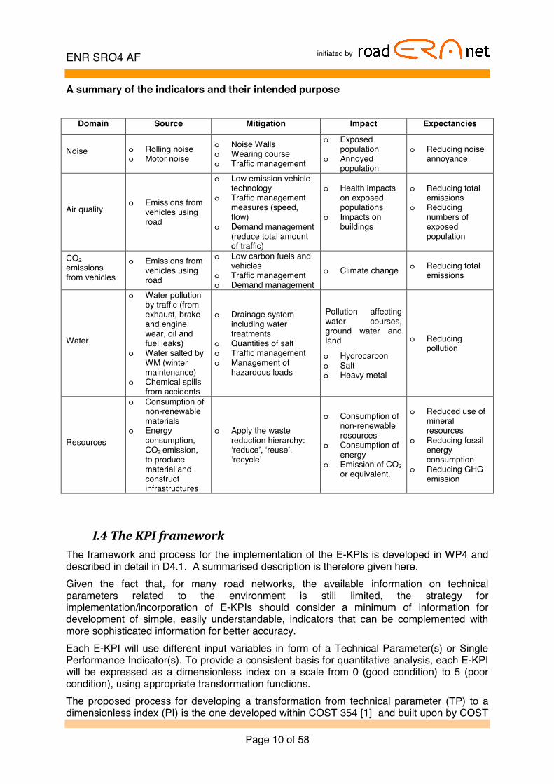

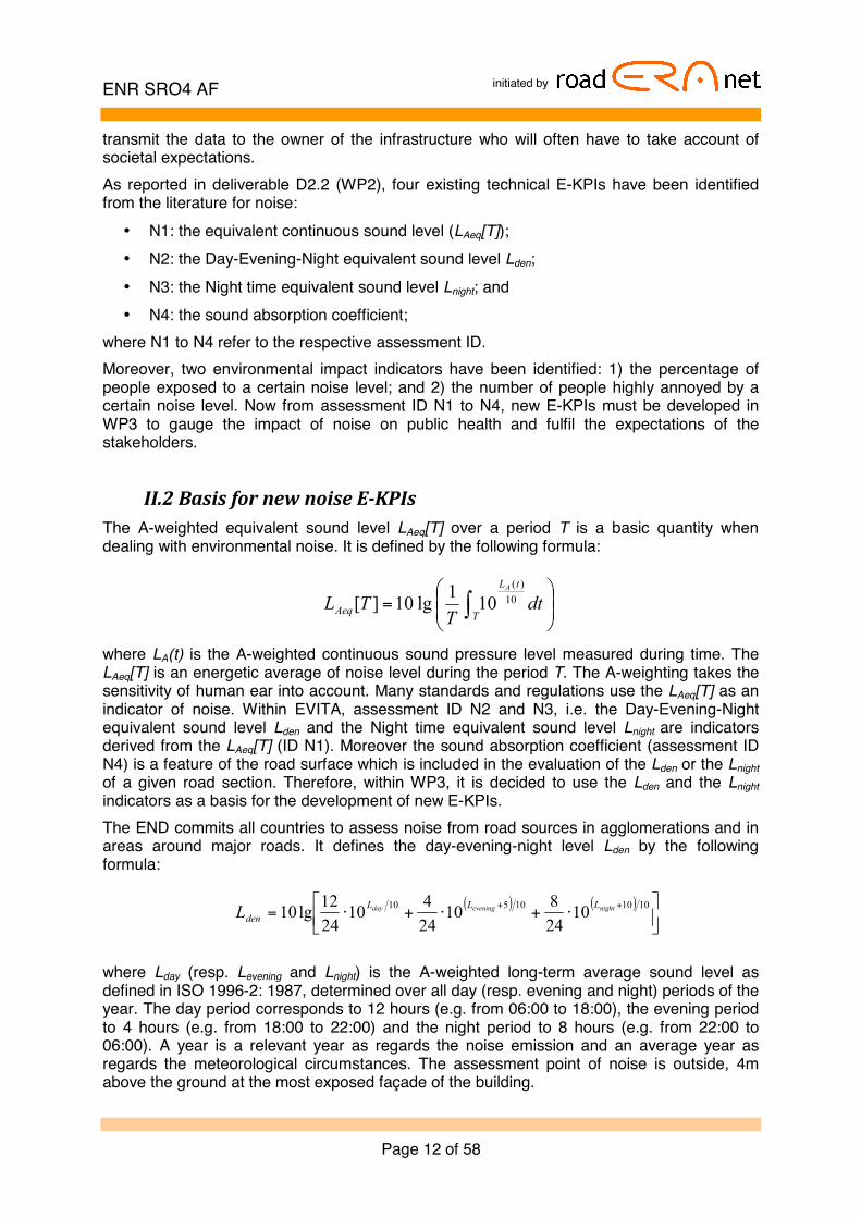


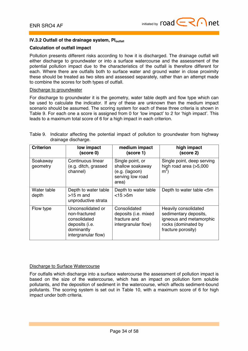


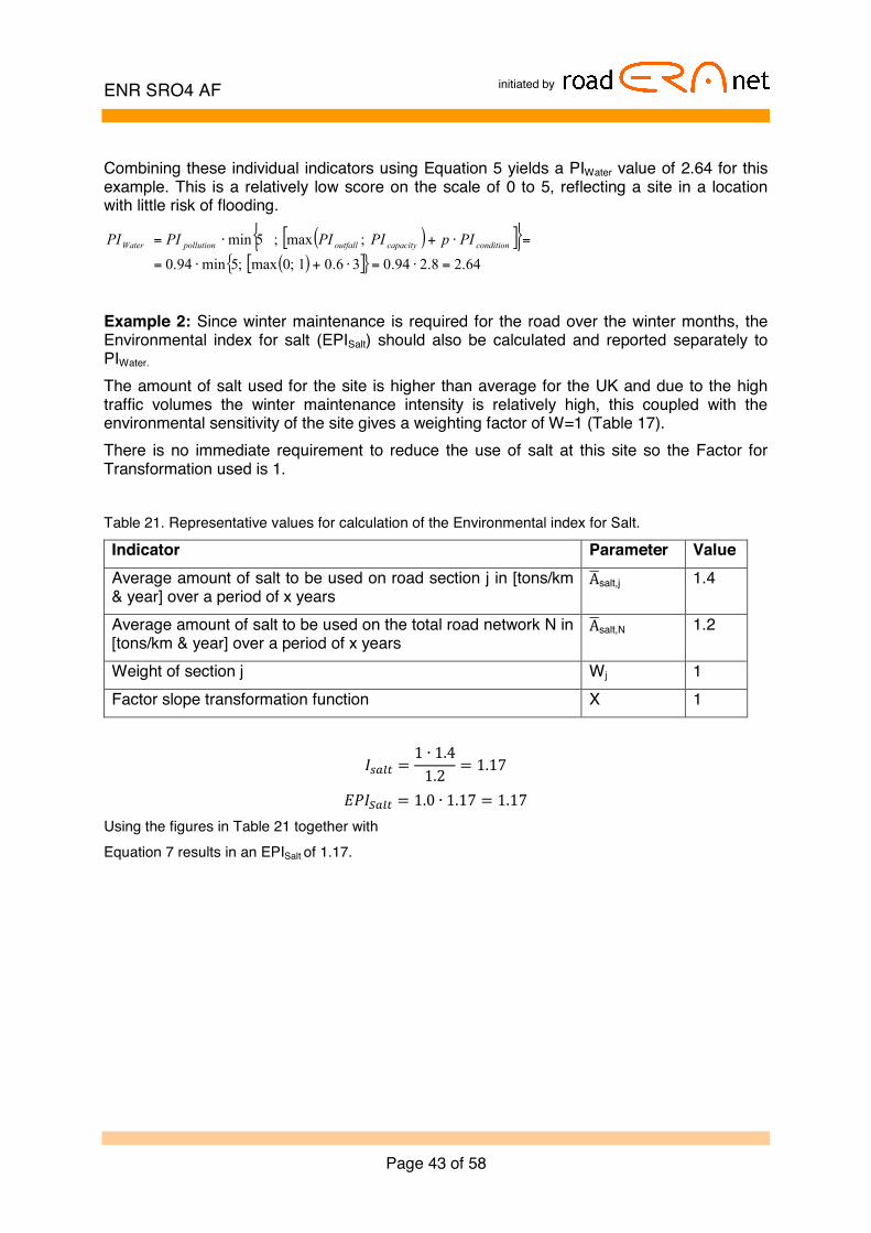


![EVITA[Version Pelicula]](https://static.documents.pub/doc/80x56/55cf864d550346484b964419/evitaversion-pelicula.jpg)


