107
| Date post: | 02-Jan-2016 |
| Category: |
Documents |
| Upload: | yolanda-hensley |
| View: | 17 times |
| Download: | 0 times |


Examples of Quantitative Support Methods from Real
World Appraisals
Jeffrey A. Johnson, MAI
Integra Realty Resources – Minneapolis / St. Paul
Tony Lesicka, MAI
Central Bank

Overview of Presentation
EXAMPLES OF TECHNIQUES AND METHODS EMPLOYED BY REAL WORLD APPRAISERS TO SOLVE UNIQUE APPRAISAL CHALLENGES USING QUANTITATIVE METHODS, TO SUPPORT THEIR OPINIONS; EXAMPLES CHOSEN ARE ALL FROM THE SALES COMPARISON APPROACH

Review of Sales Comparison Approach
SEARCH, FIND, & VERIFY RECENT SALES OF PROPERTIES SIMILAR ENOUGH TO THE SUBJECT PROPERTY TO BE CALLED AND ANALYZED AS COMPARABLES

Review of Sales Comparison Approach
IF COMPARABLE IS AN EXACT TWIN OF SUBJECT – STOP HERE;
IF NOT, MAKE A COMPARATIVE ANALYSIS OF EACH COMPARABLE SALE PROPERTY AND SUBJECT PROPERTY

Review of Sales Comparison Approach
IF SUBJECT AND COMPARABLE DIFFER SIGNIFICANTLY IN A PARTICULAR FEATURE,
THEN ONE MAKES AN ADJUSTMENT TO THE SALE PRICE OF THE COMPARABLE TO REFLECT THE FEATURES DIFFERING CONTRIBUTIONS TO VALUE FOR THE COMP AND THE SUBJECT

Review of Sales Comparison Approach
INDICATION OF SUBJECT VALUE = SALE PRICE OF COMPARABLE - CONTRIBUTING VALUE OF COMPARABLE FEATURE + CONTRIBUTING VALUE OF SUBJECT FEATURE
[AN ADDITIVE MODEL]

Review of Sales Comparison Approach
INDICATION OF SUBJECT VALUE = ADJUSTMENT FACTOR X SALE PRICE OF COMPARABLE
[A MULTIPLICATIVE MODEL]

Review of Sales Comparison Approach
IN MULTIPLICATIVE MODEL THE ADJUSTMENT FACTOR IS THE RATIO OF THE VALUE CONTRIBUTION OF THE SUBJECT FEATURE DIVIDED BY THE VALUE CONTRIBUTION OF THE COMP’S FEATURE; IN THE ADDITIVE MODEL, IT IS THE DIFFERENCE OF THE FEATURES VALUE CONTRIBUTION TO THE SUBJECT LESS THAT OF THE COMPARABLE, THAT DIFFERENCE IS ADDED TO THE SALE PRICE OF COMPARABLE

Review of Sales Comparison Approach
HOW DOES ONE COME UP WITH THESE ADJUSTMENT FACTORS? HOW DOES ONE SUPPORT THESE ADJUSTMENT FACTORS?
THAT IS WHY WE ARE HERE!

#1: Office Finish Adjustment - Industrial
THE AMOUNT OF OFFICE FINISHED SPACE IN AN INDUSTRIAL BUILDING APPRAISAL IS A VARIABLE FOR WHICH WE COMMONLY SEE AN ADJUSTMENT MADE. SOME INDUSTRIAL BUILDINGS, SUCH AS A MANUFACTURING PLANT, MAY HAVE A RELATIVELY SMALL AMOUNT OF OFFICE SPACE.SOME INDUSTRIAL BUILDINGS, SUCH AS A FLEX OR OFFICE/SHOWROOM BUILDING, MAY EVEN HAVE A MAJORITY OF ITS SPACE FINISHED AS OFFICES.

#1: Office Finish Adjustment - Industrial
WHEN A NEW INDUSTRIAL BUILDING IS BUILT IT GENERALLY COSTS MORE FOR A GREATER AMOUNT OF OFFICE FINISHED SPACE.
THIS COST DIFFERENTIAL IS AN OFTEN USED RATIONAL AS THE BASIS FOR THE ADJUSTMENT THAT IS MADE AND THIS IS OUR FIRST EXAMPLE.

#1: Office Finish Adjustment – Cost Basis
#18R-APPRAISAL PROBLEM: THE SUBJECT APPRAISAL ASSIGNMENT WAS TO ESTIMATE MARKET VALUE FOR AN EXISTING INDUSTRIAL OFFICE/WAREHOUSE PROPERTY. THE APPRAISAL WAS USED FOR REFINANCING PURPOSES. THE PROPERTY APPRAISED CONSISTED OF A 5.34 ACRE SITE IMPROVED WITH A 108,000 SQUARE FOOT OFFICE/WAREHOUSE INDUSTRIAL BUILDING THAT WAS BUILT IN 1968 WITH AN ADDITION IN 2005.

#1: Office Finish Adjustment – Cost Basis
THE COMPARABLE SALES RANGED FROM 7.5% FINISHED OFFICE SPACE TO 40.0% FINISHED.
THIS EXAMPLE SHOWS HOW ONE APPRAISER HAD ATTEMPTED TO QUANTIFY THIS OFFICE FINISH ADJUSTMENT BY RELATING HIS ESTIMATED ADJUSTMENT TO THE REPLACEMENT COSTS OF BUILDINGS WITH VARYING PERCENTAGES OF FINISH.

#1: Office Finish Adjustment – Cost Basis
THE DATE OF VALUATION WAS MAY 23, 2011.THE APPRAISER USED SIX SALES IN HIS SALES COMPARISON ANALYSIS THAT RANGED FROM 50,372 SQUARE FEET TO 192,924 SQUARE FEET. A SIGNIFICANT DIFFERENCE BETWEEN THESE COMPARABLE SALES AND THE SUBJECT PROPERTY WERE THEIR VARYING LEVELS OF OFFICE FINISH.

#1: Office Finish Adjustment – Cost Basis
This adjustment category reflects the differences in the percentage of finished office area between the subject and the comparables. Adjustments were applied to the comparables based on the differential of finished area between the comparables and the subject. Typically, office space rents for nearly double the rate of warehouse space.

#1: Office Finish Adjustment – Cost Basis
The subject property has a finished area of approximately 20% of net rentable building area. The comparables have finished area ranging from 7.5% to 40%. The table below summarizes the adjustments made to each sale based on the differences of finished area.


#1: Office Finish Adjustment – Cost Basis THE APPRAISAL THEORY BEHIND THIS TECHNIQUE IS THAT MARKET VALUE IS RELATED TO REPLACEMENT COST. THAT IS, THE GREATER THE COST FOR BUILDINGS WITH GREATER PERCENTAGES OF OFFICE SPACE, THE GREATER THE MARKET VALUES OF THOSE BUILDINGS. IN THE ABOVE CHART THE APPRAISER FIRST ESTIMATES THE LIKELY COST PER SQUARE FOOT FOR THE SUBJECT BUILDING, GIVEN ITS 20% LEVEL OF OFFICE FINISH.
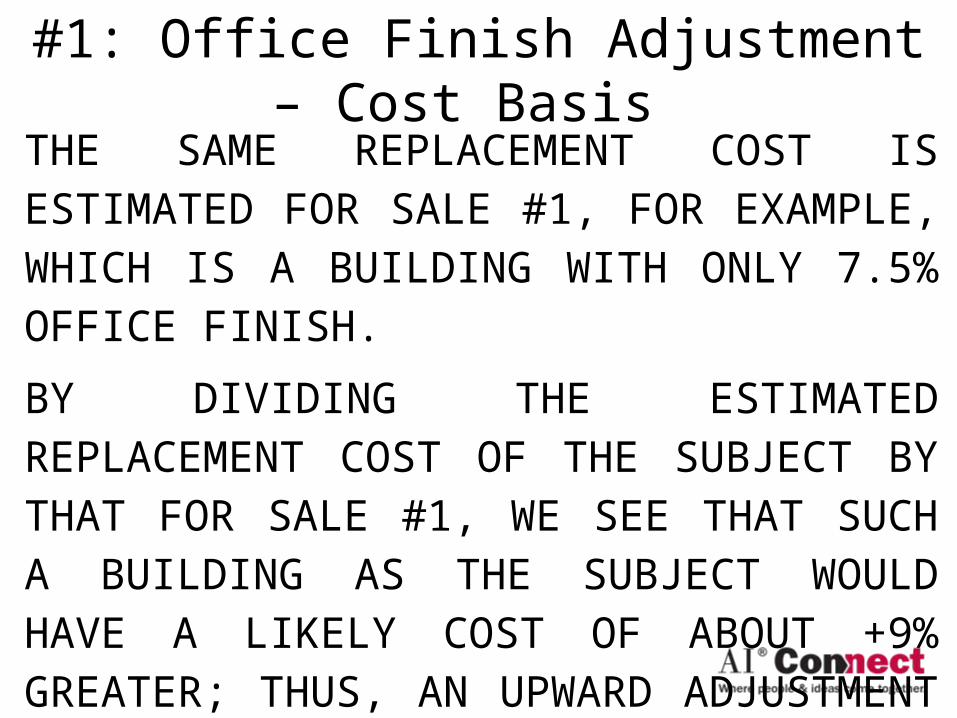
#1: Office Finish Adjustment – Cost Basis THE SAME REPLACEMENT COST IS ESTIMATED FOR SALE #1, FOR EXAMPLE, WHICH IS A BUILDING WITH ONLY 7.5% OFFICE FINISH.
BY DIVIDING THE ESTIMATED REPLACEMENT COST OF THE SUBJECT BY THAT FOR SALE #1, WE SEE THAT SUCH A BUILDING AS THE SUBJECT WOULD HAVE A LIKELY COST OF ABOUT +9% GREATER; THUS, AN UPWARD ADJUSTMENT OF +9% IS REASONED TO ESTIMATE MARKET VALUE.

#1: Office Finish Adjustment – Cost Basis THIS APPROACH IS VIEWED AS A GOOD TECHNIQUE OF ATTEMPTING TO MEASURE VALUE DIFFERENCES FOR PROPERTIES WITH VARYING DEGREES OF OFFICE FINISH. ONE SHOULD BE AWARE THAT THIS IS A LINEAR MODEL AND IT MAY NOT APPLY IF THERE IS A LARGE DEGREE OF DIFFERENCE IN THE SUBJECT AND COMPARABLE SALE BUILDINGS. THIS TECHNIQUE IS CONSIDERED TO BEST MEASURE SMALL DIFFERENCES.

#1: Office Finish Adjustment – Cost Basis IF, FOR EXAMPLE, A COMPARABLE SALE BUILDING HAD 80% OFFICE FINISH AND THE SUBJECT HAD 20%, ONE MIGHT WANT TO TEMPER THIS CALCULATED ADJUSTMENT FOR THE POSSIBLE FUNCTIONAL OBSOLESCENCE OF AN OVER-IMPROVEMENT OF TOO MUCH OFFICE FINISHED SPACE. FINALLY, SINCE THIS METHOD USES COST DIFFERENCES TO MEASURE MARKET VALUE DIFFERENCES, ONE MUST BE AWARE OF ANY FUNCTIONAL OR EXTERNAL OBSOLESCENCE ISSUES.

#1: Office Finish Adjustment – Cost Basis FUNCTIONAL OBSOLESCENCE MIGHT BE THE OVER IMPROVEMENT ISSUE OF TOO MUCH OFFICE SPACE FOR WHICH THE MARKET WILL NOT REFLECT FULLY IN VALUE, AS DISCUSSED ABOVE. THE EXTERNAL OBSOLESCENCE MIGHT BE AN ECONOMICALLY DEPRESSED OR OVER BUILT MARKET FOR WHICH COST DOES NOT EQUAL VALUE.

#2: Office Finish Adjustment – Rent Basis
#18S APPRAISAL PROBLEM: THE SUBJECT APPRAISAL ASSIGNMENT WAS TO ESTIMATE MARKET VALUE FOR AN EXISTING INDUSTRIAL OFFICE/WAREHOUSE PROPERTY. THE APPRAISAL WAS USED FOR REFINANCING PURPOSES. THE PROPERTY APPRAISED CONSISTED OF A 2.79 ACRE SITE IMPROVED WITH A 29,000 SQUARE FOOT OFFICE WAREHOUSE INDUSTRIAL BUILDING THAT WAS BUILT IN 2005. THE DATE OF VALUATION WAS MARCH 16, 2011.

#2: Office Finish Adjustment – Rent Basis
THE APPRAISER USED FIVE SALES IN HIS SALES COMPARISON ANALYSIS THAT RANGED FROM 24,408 SQUARE FEET TO 59,782 SQUARE FEET. A SIGNIFICANT DIFFERENCE BETWEEN THESE COMPARABLE SALES AND THE SUBJECT PROPERTY WERE THEIR VARYING LEVELS OF OFFICE FINISH. INDUSTRIAL BUILDINGS WILL GENERALLY SELL FOR GREATER PRICES, IF THEY HAVE A LARGER PERCENTAGE OF SPACE FINISHED FOR OFFICE USE.

#2: Office Finish Adjustment – Rent Basis
THE COMPARABLE SALES RANGED FROM 7.0% FINISHED OFFICE SPACE TO 50.2% FINISHED. APPRAISERS OFTEN HAVE TO USE INDUSTRIAL SALES THAT HAVE DIFFERENT LEVELS OF OFFICE FINISH THAN THEIR SUBJECT PROPERTY AND THEN APPLY AN OFFICE FINISH ADJUSTMENT. THIS EXAMPLE SHOWS HOW ONE APPRAISER HAD ATTEMPTED TO QUANTIFY THIS OFFICE FINISH ADJUSTMENT BY RELATING HIS ESTIMATED ADJUSTMENT TO THE NET RENTAL RATES OF BUILDINGS WITH VARYING PERCENTAGES OF FINISH.

#2: Office Finish Adjustment – Rent Basis
This adjustment category reflects the differences in the percentage of finished office area between the subject and the comparables. Adjustments are applied to the comparables based on the differential of finished area between the comparables and the subject. Typically, in this market place office space rents for nearly double the rate of warehouse space.

#2: Office Finish Adjustment – Rent Basis
The subject property has a finished area of approximately 16% of gross building area. The comparables have finished area ranging from 7% to 50%. The theory of this adjustment is that greater rental rates imply greater market value. In the table below, first the overall rental rate factor of the subject building is calculated to be 116% of the rental rate factor of just warehouse space.

#2: Office Finish Adjustment – Rent Basis
Then the same factor is calculated for each comparable sale property and the adjustment is calculated by dividing the subject factor by that of the comparable sale. The table below summarizes the adjustments made to each sale based on the differences of finished area.


#2: Office Finish Adjustment – Rent Basis THE APPRAISER DOES NOT FULLY EXPLAIN HIS METHOD SO WE WILL PRESENT OUR EXPLANATION. IN THIS PARTICULAR INDUSTRIAL MARKET IT IS COMMON FOR RENTAL RATES TO BE QUOTED ON PRICE PER SQUARE FOOT OF WAREHOUSE SPACE AND A DIFFERENT QUOTED RATE OF FINISHED OFFICE SPACE. THE RELATIONSHIP OF THESE TWO RENTAL RATES IS THAT USUALLY THE RATE FOR FINISHED OFFICE SPACE IN A BUILDING IS ABOUT DOUBLE THE WAREHOUSE RATE. THUS, THE APPRAISER REASONS THAT THE OVERALL SPACE RENTAL RATE FOR A BUILDING, LIKE THE SUBJECT, HAVING APPROXIMATELY 16% OF ITS AREA FINISHED AS OFFICE SPACE IS 1.16X

#2: Office Finish Adjustment – Rent Basis
[CALCULATED AS: 0.16(2X) + 0.84(X) = 1.16X, WHERE X REPRESENTS THE RENTAL RATE FOR WAREHOUSE SPACE].
SIMILARLY, THE OVERALL RENTAL RATE FOR A BUILDING LIKE SALE #1, WITH 35% SPACE FINISHED AS OFFICES, IS 1.35X. SO WHEN YOU CREATE AN ADJUSTMENT FACTOR BY DIVIDING THE RENTAL RATE OF THE SUBJECT (1.16X) BY THE RENTAL RATE OF SALE #1 (1.35X) YOU GET A FACTOR OF 0.857, WHICH IS RESTATED AS A DOWNWARD ADJUSTMENT OF -14.3%.

#2: Office Finish Adjustment – Rent Basis
THIS METHOD WORKS BEST IF THERE IS NOT TOO MUCH DIFFERENCE IN LEVELS OF OFFICE FINISH. IF THERE IS A SUBSTANTIAL DIFFERENCE IN LEVELS OF OFFICE FINISH THE READER IS CAUTIONED THAT THIS CALCULATED ADJUSTMENT MIGHT NOT ACCURATELY REFLECT THE DIFFERENCE IN MARKET PRICES FOR THE SAME REASONING WE SET FORTH IN EXAMPLE #18R.

#3: Unit Mix Adjustment - Apartments
A very common real estate property type is Apartments.
Many apartment appraisals will have comparable sales that differ from the subject property in Unit Mix.
How does one adjust for these differences?

#3: Unit Mix Adjustment - Apartments
“Unit Mix” is merely a categorical variable; not a measurement variable, neither discrete or continuous
Is a 3-Bedroom unit worth 150% of a 2-Bedroom unit?
Is it worth 300% of a 1-Bedroom unit?

#3: Unit Mix Adjustment - Apartments #18U - APPRAISAL PROBLEM: THE SUBJECT APPRAISAL ASSIGNMENT WAS TO ESTIMATE THE CURRENT MARKET VALUE OF A 30-UNIT MARKET RATE APARTMENT PROPERTY. THE PROPERTY APPRAISED CONSISTED OF A 1.46 ACRE SITE IMPROVED WITH A 30-UNIT APARTMENT BUILDING BUILT IN 1973. IT WAS 93% OCCUPIED AND CONSISTED OF 24 ONE-BEDROOM UNITS AND 6 TWO-BEDROOM UNITS. THE APPRAISAL WAS MADE FOR MORTGAGE FINANCING PURPOSES. THE DATE OF VALUATION WAS JUNE 23, 2011.

#3: Unit Mix Adjustment - Apartments THE APPRAISER USED EIGHT SALES OF APARTMENT PROPERTIES IN HER SALES COMPARISON ANALYSIS. ONE DIFFERENCE BETWEEN THESE COMPARABLE SALES AND THE SUBJECT PROPERTY WAS THEIR UNIT MIX. THE SUBJECT PROPERTY HAD MOSTLY ONE BEDROOM UNITS; 80% (24 ÷ 30 = 0.80) OF ITS TOTAL UNITS. THE COMPARABLE SALES VARIED IN THEIR UNIT MIX MAKEUPS. SALE #4 CONSISTED OF AN APARTMENT WHERE APPROXIMATELY 89% (40 ÷ 45 = 0.8888) OF ITS UNITS WERE ONE-BEDROOM UNITS.

#3: Unit Mix Adjustment - Apartments HOWEVER, SALE #7 CONSISTED OF AN APARTMENT WHERE 100% OF ITS UNITS WERE TWO-BEDROOM UNITS.IT IS COMMON FOR APPRAISERS TO HAVE TO USE SALES OF APARTMENT PROPERTIES THAT VARY IN THEIR UNIT MIX FROM THE SUBJECT APARTMENT PROPERTY BEING APPRAISED. THIS EXAMPLE SHOWS HOW ONE APPRAISER HAD ATTEMPTED TO QUANTIFY THIS ADJUSTMENT FOR VARYING UNIT MIXES IN AN APPRAISAL OF AN APARTMENT PROPERTY.

#3: Unit Mix Adjustment - Apartments This adjustment category accounts for the differences in unit mix of the subject and comparable properties recognizing that the more bedrooms a multifamily property contains, the higher potential rent it can generally achieve. The expectation is that a property with a greater percentage of two- and three-bedroom units should sell for a higher per-unit price than a complex with a greater percentage of efficiencies and one-bedroom units. We find in this market that efficiency units typically rent for about 85% of the rent that otherwise similar one-bedroom units achieve.

#3: Unit Mix Adjustment - Apartments Two-bedroom rents are generally about +25% higher than one-bedroom units, and three-bedroom rental rates are approximately 60% higher than one-bedroom units. These observed rental differences are summarized as follows:
Efficiency Units: 85% of a one bedroom
One Bedroom Units: 100% of a one bedroom
Two Bedroom Units: 125% of a one bedroom
Three Bedroom Units: 160% of a one bedroom

#3: Unit Mix Adjustment - Apartments To initiate the adjustment process, the subject and comparable sales are converted to a one-bedroom-equivalency utilizing the preceding scale. To make this calculation, the total number of each unit type is multiplied by its corresponding rent percentage differential. Each of these figures is then added together and divided by the total number of dwelling units at the property. The result is a one-bedroom equivalent factor for the subject and each comparable property.

#3: Unit Mix Adjustment - Apartments For example, the subject property, which consists of 24 one-bedroom units and 6 two-bedroom units, can be expressed on this one-bedroom-rent-equivalent scale as being equivalent to an apartment with average units having rents of 1.05 times that of a typical one-bedroom unit {e.g. [(0 x 0.85) + (24 x 1.00) + (6 x 1.25) + (0 x 1.60)] ÷ 30 = 1.05}. Then the relationship between the subject and each comparable one-bedroom-equivalency factor, if any, is the final adjustment factor, expressed as a percentage.


#3: Unit Mix Adjustment - Apartments AUTHORS’ REVIEW COMMENTS: IN THIS APPRAISAL THAT WAS MADE FOR MORTGAGE FINANCING PURPOSES, THE APPRAISER USED A RENT BASED METHOD TO ASSIST IN HER EVALUATION OF HOW THE DIFFERING UNIT MIXES IMPACTED THE MARKET VALUE OF THIS PROPERTY. WE FIND THAT MOST ADJUSTMENTS THAT WE SEE FOR APARTMENT UNIT MIX ARE SUPPORTED ON A DIFFERENCE IN AVERAGE UNIT SQUARE FOOTAGES. WE OBSERVE THAT THIS METHOD IS BASED ON AN ECONOMIC SCALE FOR THE ADJUSTMENT.
#4: Time/Market Conditions Adjustment - Apartment Property
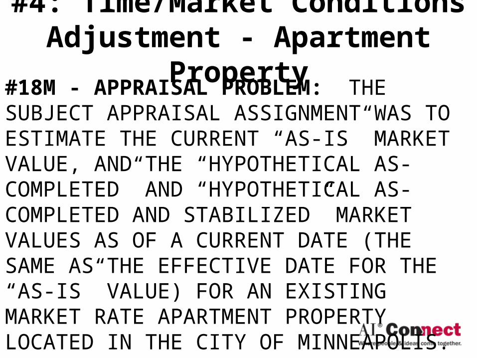
#18M - APPRAISAL PROBLEM: THE SUBJECT APPRAISAL ASSIGNMENT WAS TO ESTIMATE THE CURRENT “AS-IS” MARKET VALUE, AND THE “HYPOTHETICAL AS-COMPLETED” AND “HYPOTHETICAL AS-COMPLETED AND STABILIZED” MARKET VALUES AS OF A CURRENT DATE (THE SAME AS THE EFFECTIVE DATE FOR THE “AS-IS” VALUE) FOR AN EXISTING MARKET RATE APARTMENT PROPERTY LOCATED IN THE CITY OF MINNEAPOLIS. THE APPRAISAL WAS USED FOR REFINANCING PURPOSES. THE PROPERTY APPRAISED CONSISTED OF A 4.5 ACRE SITE IMPROVED WITH A 100-UNIT APARTMENT PROPERTY
#4: Time/Market Conditions Adjustment - Apartment Property
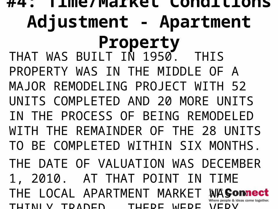
THAT WAS BUILT IN 1950. THIS PROPERTY WAS IN THE MIDDLE OF A MAJOR REMODELING PROJECT WITH 52 UNITS COMPLETED AND 20 MORE UNITS IN THE PROCESS OF BEING REMODELED WITH THE REMAINDER OF THE 28 UNITS TO BE COMPLETED WITHIN SIX MONTHS.THE DATE OF VALUATION WAS DECEMBER 1, 2010. AT THAT POINT IN TIME THE LOCAL APARTMENT MARKET WAS THINLY TRADED. THERE WERE VERY FEW ARM’S LENGTH SALES AVAILABLE FOR APPRAISERS TO USE IN THEIR SALES COMPARISON ANALYSIS.

#4: Time/Market Conditions Adjustment - Apartment Property
APPRAISERS WERE HAVING TO USE SOME OLDER SALES AND THEN APPLY A MARKET CONDITIONS ADJUSTMENT. THIS EXAMPLE SHOWS HOW ONE APPRAISER HAD ATTEMPTED TO QUANTIFY THIS CHANGING MARKET CONDITIONS ADJUSTMENT.

#4: Market Conditions - ApartmentThere is no index for the local real estate market to There is no index for the local real estate market to show pricing movement through time for this show pricing movement through time for this particular multi-family property sub-market. particular multi-family property sub-market.
However, since the local real estate market has However, since the local real estate market has become more dependent on the national financing become more dependent on the national financing market and also as many investors are seeking to market and also as many investors are seeking to acquire investments in a larger geographic area, acquire investments in a larger geographic area, many even on a national basis, we have reviewed a many even on a national basis, we have reviewed a national property pricing index and present national property pricing index and present information on it in this section. information on it in this section.

#4: Market Conditions - ApartmentThe Moodys/REAL Commercial Property Index The Moodys/REAL Commercial Property Index (CPPI) is a periodic same-property round-trip (CPPI) is a periodic same-property round-trip investment price change index of the United States investment price change index of the United States commercial investment property market based on commercial investment property market based on data from the Massachusetts Institute of data from the Massachusetts Institute of Technology (MIT) Center for Real Estate industry Technology (MIT) Center for Real Estate industry partner Real Capital Analytics, Inc. (RCA). partner Real Capital Analytics, Inc. (RCA).

#4: Market Conditions - Apartment

#4: Market Conditions - Apartment

#4: Market Conditions - ApartmentAn alternative way to analyze this data is to calculate the change from quarter-to-quarter.
By dividing the current quarterly index by the prior quarterly index we obtain an indication of the quarterly rate of pricing change.
Since many real estate investment market participants usually quote pricing rates of change on an annual percentage basis,

#4: Market Conditions - Apartment
we find this quarterly rate of change analysis to be helpful and present the following graph showing the indicated quarterly rates of change through time for this national apartment market data.

#4: Market Conditions - Apartment

#4: Market Conditions - ApartmentTo analyze our local apartment market for pricing movement we have assembled information on how average apartment rents have changed over time and also how average apartment vacancy rates have changed over time.
The value of apartment properties is a function of not only the economic performance of the properties but also the capitalization rate that buyers are using to acquire properties.

#4: Market Conditions - Apartment
This chart also shows the average capitalization rate that is found in the Korpacz Real Estate Investor Survey, which is a quarterly publication of Price Waterhouse Coopers.
We have used this information along with our estimate of typical expenses for metro area apartments to calculate an implied value change from quarter to quarter.

#4: Market Conditions - Apartment

#4: Market Conditions - Apartment
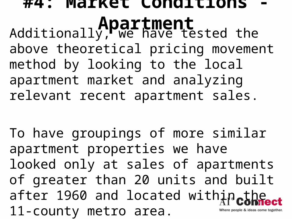
#4: Market Conditions - ApartmentAdditionally, we have tested the above theoretical pricing movement method by looking to the local apartment market and analyzing relevant recent apartment sales.
To have groupings of more similar apartment properties we have looked only at sales of apartments of greater than 20 units and built after 1960 and located within the 11-county metro area.

#4: Market Conditions - ApartmentWe have taken this sales data from a professional appraiser verified database of sale transactions. We find the following statistical data to also be of help in estimating rates of pricing change through time for the changing market conditions within our local apartment market. We have used the same time intervals identified in the above theoretical method and have grouped the apartment sales from our database of professional appraiser verified sales into groups based on the timing of the date each sale was closed.

#4: Market Conditions - Apartment

#4: Market Conditions - ApartmentThe sales analyzed in this appraisal took place from May 2008 to March 2010. Based on our research and experience we conclude that for this evaluation of the subject property and for the comparable sales selected for this comparative analysis that the local apartment market was generally strengthening with prices appreciating during the period from the third quarter of 2004 through the third quarter of 2006 at a rate of about +10% per year; we will use a rate of +2.5% per quarter for that period.

#4: Market Conditions - ApartmentWe conclude that prices were generally stable during the period from the fourth quarter of 2006 through the third quarter of 2008 and we will use a rate of +0.0% per quarter for that period. However, beginning in the fourth quarter of 2008 through the fourth quarter of 2009 we are of the opinion that prices have been depreciating and we will use a rate of decline of -8% per year, or about -2.0% per quarter.

#4: Market Conditions - Apartment
We are of the opinion that beginning with the first quarter of 2010 through the current period that prices have stabilized and remained level at these reduced lower levels and we will use a rate of +0.0% per quarter for this most recent period. These conclusions of market condition rates of pricing changes will be applied to each of our comparable sales to express their transaction prices as of our date of evaluation.

#5: Shape Adjustment – Retail Land
#16J - APPRAISAL PROBLEM: THE SUBJECT APPRAISAL ASSIGNMENT WAS TO ESTIMATE THE DIMINUTION IN MARKET VALUE RESULTING FROM A PARTIAL TAKING OF LAND FROM A COMMERCIALLY ZONED PROPERTY. THE PROPERTY APPRAISED CONSISTED OF A TWO-LOT TOTAL SITE WITH AN AREA OF 37,168 SQUARE FEET, BEFORE THE PARTIAL TAKING. THE DATE OF VALUATION WAS JUNE 18, 2010. THE APPRAISER USED NINE SALES OF COMMERCIAL LAND PARCELS IN HIS SALES COMPARISON ANALYSIS.

#5: Shape Adjustment – Retail LandONE DIFFERENCE BETWEEN THESE COMPARABLE SALES AND THE SUBJECT PROPERTY WAS SHAPE AND ALSO THE SHAPE OF THE SUBJECT PROPERTY CHANGED AS A RESULT OF THIS PARTIAL TAKING. PRIOR TO THE TAKING IT WAS NEARLY RECTANGULAR AND AFTER THE TAKING IT WAS TRIANGULAR. IT IS NOT UNCOMMON FOR APPRAISERS TO HAVE TO USE COMMERCIAL LAND SALES THAT HAVE DIFFERENT SHAPES IN THEIR COMPARATIVE ANALYSIS. THIS EXAMPLE SHOWS HOW ONE APPRAISER HAD ATTEMPTED TO QUANTIFY THIS ADJUSTMENT FOR A TRIANGULATED SHAPE IN AN APPRAISAL WHERE THE CHANGE IN SHAPE WAS A FOCUS OF THIS EVALUATION.

#5: Shape Adjustment – Retail LandShape: This adjustment category is also a part of the physical characteristics adjustment that generally reflects differences in the shape of the parcels and how this feature relates to development utility and value.The following exhibit shows how the shape of this land has been changed by this project. The image on the left is a depiction of how this property was configured Before the Taking and the image on the right shows the After Taking configuration.

Before Taking Parcel Configuration After Taking Parcel Configuration

#5: Shape Adjustment – Retail LandThe image on the left is a plat map of the property Before the Taking. This property consisted of two lots at the corner that together formed a nearly rectangular redevelopment tract. The shape of the subject property has been changed by this partial taking. The image on the right is from the right-of-way taking map. That area that is cross-hatched is the area of the partial taking. Before the Taking this property was nearly rectangular in shape. After the Taking this property has been made into a triangular shape at its northern end.

#5: Shape Adjustment – Retail Land
In the developing Victor Gardens area within the neighboring city of Huggeo the retail land market has been relatively active and we find an example that helps us quantify how shape can impact pricing.

#5: Shape Adjustment – Retail Land

#5: Shape Adjustment – Retail LandThe parcels labeled as Sale #4 & #5 are two land sales that were analyzed in our Before Taking evaluation. Sale #4 is the 43,296 square foot rectangular parcel that was purchased on November 30, 2007 for development of a Blue Heron restaurant. Its price was $14.44 per square foot. Sale #5 is the 39,574 square foot corner lot that was purchased on January 14, 2008 for development of an M & I Bank. Its price was $16.42 per square foot. The premium paid for the corner location appears to be about +14% ($16.42 ÷ $14.44 = 1.137, rounded to and restated as +14%).

#5: Shape Adjustment – Retail LandSale #A is a triangular shaped flag-lot parcel having a total land area of about 43,124 square feet. It was purchased on January 31, 2007 for development of a bank at a price of about $10.58 per square foot. Comparing Sale #A to Sale #4 we find two similar sized land parcels (Land Area: Sale #4 – 43,296 square feet; Sale #A – 43,124 square feet) that sold at about the same time (Date of Sale: Sale #4 – Nov. 30, 2007; Sale #A – Jan. 31, 2007). Both sale parcels are zoned PUD.

#5: Shape Adjustment – Retail LandBoth sale parcels are located at the same commercial intersection and each is one lot removed from the corner. Both sale parcels have similar visibility from County Road 8 (Frenchman Road). However, the parcels do not have the same shape; Sale #4 is a rectangular land parcel and Sale #A is a triangular shaped flag-lot land parcel. A comparison of their prices demonstrates a differential for shape of about -27% ($10.58 ÷ $14.44 = 0.733, rounded to and restated as -27%).
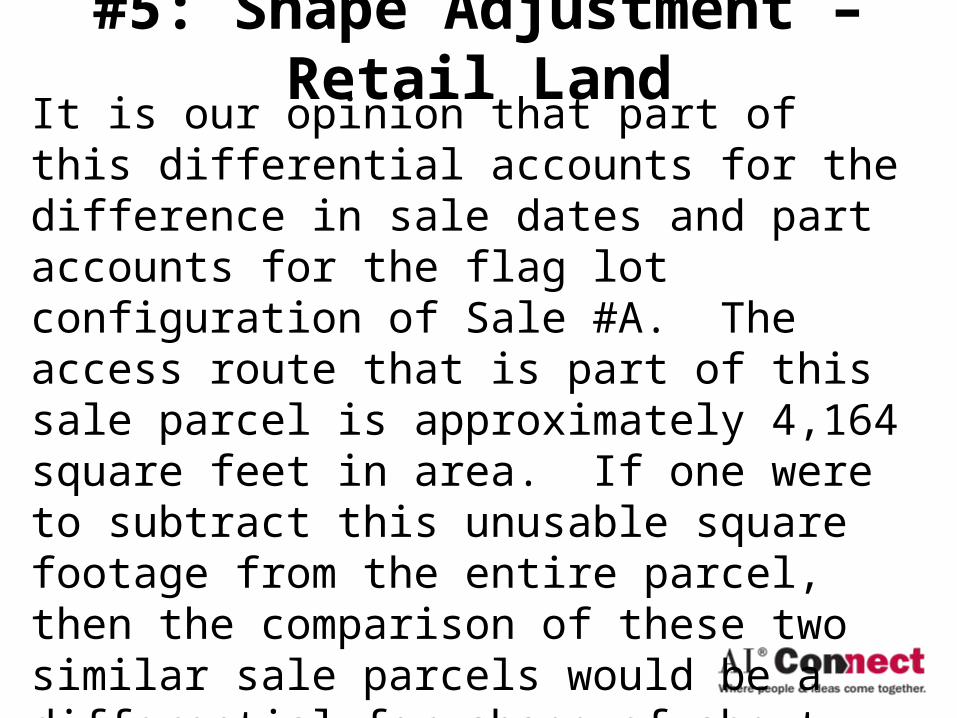
#5: Shape Adjustment – Retail LandIt is our opinion that part of this differential accounts for the difference in sale dates and part accounts for the flag lot configuration of Sale #A. The access route that is part of this sale parcel is approximately 4,164 square feet in area. If one were to subtract this unusable square footage from the entire parcel, then the comparison of these two similar sale parcels would be a differential for shape of about –19% ($11.71 ÷ $14.44 = 0.811, rounded to and restated as -19%).

#5: Shape Adjustment – Retail Land
If one were to draw a diagonal line from the northwest corner of the subject remainder parcel to the southeast corner, the result would be a triangular shaped remainder parcel on the southwest side of that line. The image below shows such a triangulation of the remainder subject parcel in this drawing.


#5: Shape Adjustment – Retail Land
However, the subject parcel is not exactly reduced to a triangular shape, like the example from the paired sales on the prior page of this report. The subject remainder parcel also includes all of the land area located northeast of this diagonal line but not that area that is cross-hatched.

#5: Shape Adjustment – Retail LandThus, we are of the opinion based on this paired sales comparison and our experience as a real estate appraiser that a triangular shaped lot would sell for a price of about 15% to 25% less than the price of an otherwise similar, yet rectangular shaped lot. From the above analysis and based upon our experience, we will make a downward adjustment of minus 15% to account for the somewhat triangular shape of the northern portion of the subject property in its After Taking configuration.

#5: Shape Adjustment – Retail LandAUTHORS’ REVIEW COMMENTS: IN THIS APPRAISAL THAT WAS MADE FOR A PARTIAL TAKING THAT RESULTED IN A SOMEWHAT TRIANGULATED SHAPE FOR THE SUBJECT PROPERTY, THE APPRAISER USED THE PAIRED SALES METHOD TO ASSIST IN HIS EVALUATION OF HOW THE CHANGE IN SHAPE IMPACTED THE MARKET VALUE OF THIS PROPERTY. WE DO NOTICE AND APPRECIATE THE APPRAISER’S CHOICE OF WORDS WHERE HE SAYS, “FROM THE ABOVE ANALYSIS AND BASED UPON OUR EXPERIENCE (EMPHASIS ADDED), WE WILL MAKE A DOWNWARD ADJUSTMENT OF …”

#5: Shape Adjustment – Retail Land
WE THINK IT IS IMPORTANT THAT APPRAISERS ALWAYS LOOK TO RECENT SALES BUT ALSO GIVE CONSIDERATION TO THEIR EXPERIENCE IN MAKING THEIR CONCLUSIONS. WE THINK THIS IS PARTICULARLY IMPORTANT WHEN USING THE PAIRED SALES APPROACH SINCE WE NEVER DO HAVE A PERFECTLY MATCHED PAIRING AND ALSO AS IN THIS EXAMPLE THIS WAS ONLY ONE SUCH PAIRING THAT WAS STUDIED.

#6: Land-Building Ratio Adjustment – Industrial Property
#18W - APPRAISAL PROBLEM: THE SUBJECT APPRAISAL ASSIGNMENT WAS TO ESTIMATE THE DIMINUTION IN MARKET VALUE RESULTING FROM A PARTIAL TAKING OF LAND FROM AN EXISTING INDUSTRIAL OFFICE/WAREHOUSE PROPERTY LOCATED IN MINNEAPOLIS. THE PROPERTY APPRAISED CONSISTED OF A 12.45 ACRE SITE IMPROVED WITH AN 153,559 SQUARE FOOT OFFICE WAREHOUSE INDUSTRIAL BUILDING THAT WAS BUILT IN 1955 AND RENOVATED IN 1990. THE DATE OF VALUATION WAS APRIL 2, 2008.

#6: Land-Building Ratio Adjustment – Industrial Property
THE APPRAISER USED SIX SALES IN HIS SALES COMPARISON ANALYSIS. ONE DIFFERENCE BETWEEN THESE COMPARABLE SALES AND THE SUBJECT PROPERTY WERE THEIR VARYING LAND-TO-BUILDING RATIOS. INDUSTRIAL BUILDINGS MAY GENERALLY SELL FOR GREATER PRICES IF THEY HAVE LARGER LAND-TO-BUILDING RATIOS, DEPENDING ON THE INCREMENTAL INCREASE IN VALUE FOR SITE SIZE AS DETERMINED BY THE MARKET. THE COMPARABLE SALES HAD LAND-TO-BUILDING RATIOS RANGING FROM 1.57:1 TO 4.78:1, WITH THE SUBJECT AT 3.53:1 IN ITS BEFORE TAKING CONFIGURATION AND

#6: Land-Building Ratio Adjustment – Industrial Property
3.11:1 IN THE AFTER THE TAKING CONFIGURATION. IT IS NOT UNCOMMON FOR APPRAISERS TO HAVE TO USE INDUSTRIAL SALES THAT HAVE DIFFERENT LAND-TO-BUILDING RATIOS THAN THEIR SUBJECT PROPERTY AND THEN APPLY AN ADJUSTMENT FOR THE DIFFERENCES. THIS EXAMPLE SHOWS HOW ONE APPRAISER HAD ATTEMPTED TO QUANTIFY THIS ADJUSTMENT FOR VARYING LAND-TO-BUILDING AREA RATIOS.

#6: L-B Ratio Adjustment – IndustrialLoss of Expansion Capabilities and Change in Land-to-Building Area Ratio. The partial taking results in a lesser land-to-building area ratio and a lesser ability to expand the existing industrial facility. Before this partial taking the land-to-building ratio for this subject property was 3.53-to-1 and after the partial taking that ratio was reduced to 3.11-to-1. To estimate the Twin Cities Industrial Market pricing reaction to having less land area available for expansion of larger industrial buildings, we have assembled a database of 108 sales of industrial buildings larger than 80,000 square

#6: L-B Ratio Adjustment – Industrialfeet that sold during the period of from January 2006 through November 2008. The range of gross building area is from 80,400 to 241,298 square feet with an average of 134,339 square feet and a median of 120,099 square feet. The subject building has a total area of 153,559 square feet. These sales occurred from January 5, 2006 to November 25, 2008. Our date of evaluation for this appraisal is April 2, 2008. A measure of the expansion potential for industrial properties is the Land-to-Building Area Ratio, or commonly just the land/building ratio.

#6: L-B Ratio Adjustment – IndustrialThis ratio is calculated by dividing the land area, in square feet, by the gross building area, in square feet. This ratio gives the amount of land for each square foot of gross building area. The ratio for the subject property before the taking was 3.53. These sales exhibited land/building ratios averaging 2.92 and a median of 2.72. A summary chart of these sale properties is included in the Addendum of this report. We have sorted and then grouped these sales by their land-to-building ratios and prepared the following summary chart:

#6: L-B Ratio Adjustment – Industrial

#6: L-B Ratio Adjustment – IndustrialThis chart demonstrates that sale prices for these properties tend to be greater as the land/building ratio increases. This is as one would suspect that land size in relation to building size does matter. The net effect of this partial taking is to reduce the expansion capability of this property. Before the taking the land/building ratio for the subject property was about 3.53-to-1. It had been offered for sale and most potential buyers who looked at this property were interested in the expansion capability of this property.

#6: L-B Ratio Adjustment – IndustrialAfter the taking this site is reduced to an effective land/building ratio of about 3.11-to-1. The chart above indicates that the sales with land/building ratios between 2.0 and 2.99 sold at a median price of $48.45 per square foot. Industrial properties with land/building ratios between 3.0 and 3.99 sold at a median price of $61.98 per square foot. This market data indicates that a reduction in land/building ratio of 1.0 results in a loss of -21.83%, as shown below:

#6: L-B Ratio Adjustment – Industrial
The change in land/building ratio of the subject is less than 1.0 and is only a reduction of about 0.42 (3.53 less 3.11). The Before Condition land/building ratio is 3.53:1 and the After Condition land/building ratio is 3.11. Based on the above, the value loss indicated for the subject can be estimated as 9.17% (21.83% x 0.42).

#6: L-B Ratio Adjustment – IndustrialAs we can see from the above chart, this industrial market is price sensitive to this issue. As a measure of how this change could impact the value of the subject property we have merely averaged the prices of the sale properties around each of these two land/building ratios. In the following chart the grouping on the left is the immediate twenty properties with land/building ratios less than the 3.53 ratio of the subject property and also the immediate twenty properties with land/building ratios greater than that of the subject property.

#6: L-B Ratio Adjustment – IndustrialThis grouping has a median land/building ratio of 3.53-to-1 and a median sale price per square foot of gross building area of about $65.13. The grouping on the right is the immediate twenty sales with land/building ratios less than 3.11 and also the immediate twenty sales with a ratio greater than 3.11. This grouping has a median land/building ratio of 3.11-to-1 and a median sale price per square foot of gross building area of about $53.65, or approximately -17.6% less than the price of the other grouping.


#6: L-B Ratio Adjustment – IndustrialThe above method is a relatively simple analysis that measures this market’s pricing impact as it would relate to a drop in land/building ratios of from 3.53-to-1 down to a ratio of 3.11-to-1.
Another way of looking for such a pricing relationship is to start by preparing a scatter plot graph. The following graph depicts this relationship of prices paid for larger industrial buildings and their land/building ratios.


#6: L-B Ratio Adjustment – IndustrialThis graph shows how the land/building ratio (plotted on the horizontal X-axis) is related to sale price per square foot of gross building area (plotted on the vertical Y-axis). From this graph we can again see that there is a definite relationship that exists in this segment of the industrial market, at this time. Land/Building ratio does appear to have a positive correlation with sale price per square foot. The line that best fits this data is called the least squares regression line.

#6: L-B Ratio Adjustment – IndustrialWe have used this regression statistical analysis as another method to help measure this market pricing relationship. The least squares regression line that best fits this data using only the land/building ratio variable is set forth below:Price = $25.9450 + $8.5449 x (Land/Building Ratio)The coefficient for the land/building ratio (approximately $8.54 for each integer change in land/building ratio) was found to be quite significant with a t-statistic of 5.430744 and a p-Value of only 0.00000036.

#6: L-B Ratio Adjustment – IndustrialThe t-statistic and the p-Value are inversely related in that if the t-statistic is relatively high then the p-Value will be relatively low. In this example a t-statistic of about 5.43 is quite high and it resulted in an extremely low p-Value of only 0.00000036. The p-Value is actually a probability value. In this case it is a probability well less than one percent (0.01); in fact, a small fraction of one percent (3.6 millionths of one percent). The p-Value gives a probability answer to the question of, if this independent variable (land-to-building area ratio)

#6: L-B Ratio Adjustment – Industrialwere really unrelated to the dependent variable (price per square foot) what is the chance that we would have gotten the reported t-statistic (or something greater) for this coefficient ($8.24). Since in this example the t-statistic is relatively high and the p-Value is relatively low we can then say that this result (a coefficient of about $8.54 for the Land-to-Building Area Ratio variable) is statistically significant. If we apply this result to a property with a land/building ratio of 3.53, a price of $56.11 per square foot is indicated and

#6: L-B Ratio Adjustment – Industrialif we apply it to a property with a land/building ratio of 3.11 we arrive at an indication of $52.52 per square foot, or a price reduced by about 6.4%.One can also perform this analysis using multiple variables. The least squares regression line that best fits this data using not only the land/building ratio variable but also the gross building area and date of sale variables is set forth below:Price = -$187.52 + -$0.000120 x (Gross Building Area) + $7.316 x (Land/Building Ratio) + $0.00595 x (Date of Sale)

#6: L-B Ratio Adjustment – IndustrialThe coefficient for the land/building ratio (approximately $7.32 for each integer change in land/building ratio) was again found to be quite significant with a t-statistic of 4.62345 and a p-Value of only 0.0000109. Again, we see a relatively high t-statistic and a relatively low p-Value. Which means that if the land-to-building area ratio variable were really unrelated to the Price per Square Foot variable in this market then the probability of us obtaining a t-statistic as great, or greater, than we did for the Land-to-Building Area

#6: L-B Ratio Adjustment – IndustrialRatio would have a small fraction of one percent (1.109 ten-thousandth). Thus, we conclude that this result is statistically significant. If we apply this result to a property with a gross building area of 153,559 square feet, like the subject, a land/building ratio of 3.53, and a date of sale of April 2, 2008, then a price of $55.19 per square foot is indicated. And if we apply it to a similar property with a land/building ratio of 3.11 we arrive at an indication of $52.12 per square foot, or a price reduced by about 5.6%.

#6: L-B Ratio Adjustment – IndustrialBased on our analyses we find four indications of diminution in market value for this change in land-to-building ratio; they are -5.6% of value using a multiple variable linear regression model, -6.4% of value using a single variable linear regression model, -9.2% using the charting by groups method, and -17.6% of value by using a market averaging method applied to the market prices sorted by land/building ratio groups. We find the regression methods to be better indications and conclude to a diminution in value of -6%.

#6: L-B Ratio Adjustment – IndustrialAUTHORS’ REVIEW COMMENTS: IN THIS APPRAISAL THAT WAS MADE FOR A PARTIAL TAKING THAT RESULTED IN A LESSER LAND-TO-BUILDING RATIO FOR THE SUBJECT PROPERTY, THE APPRAISER USED FOUR SEPARATE METHODS TO ATTEMPT TO EVALUATE HOW AN APPROXIMATELY 12% REDUCTION (3.11 ÷ 3.53 = 0.881, ROUNDED TO AND RESTATED AS -12%) IN LAND-TO-BUILDING RATIO WOULD IMPACT THE MARKET VALUE BY -6%. THE SECOND TWO METHODS ARE STATISTICAL EXAMPLES AND THE FIRST TWO METHODS ARE SIMPLY SURVEYING THE DATA AND SEPARATING IT INTO TWO GROUPS CENTERED ABOUT THE TWO DIFFERENT LAND-TO-BUILDING RATIOS.

#6: L-B Ratio Adjustment – Industrial
WE DO LIKE THAT THE APPRAISER USED MULTIPLE METHODS TO MEASURE THIS IMPACT. BUT WE ALSO LIKE THE FACT THAT THERE WAS A GOOD RECONCILIATION OF THE METHODS TO CONCLUDE TO AN ADJUSTMENT FACTOR.

Presenters Concluding Remarks• Thanks for attending
• We are collecting examples like those shown in this presentation; if you have any to share please contact us at [email protected]; [email protected];
• Questions and Comments


