87

EXAMPLES OF THE APPLICATION OF THE VLF-R METHOD TO PROSPECTING BEDROCK STRUCTURES

by

S.-E. Hjelt, J.V. Heikka, T.K. Pernu and E.I.O. Sandgren

Hjelt, S.-E., Heikka, J.V., Pernu, T.K. & Sandgren, E.1.0., 1990. Examples of the application of the VLF-R method to prospecting bedrock structures . Geologian tutkimuskeskus, Tutkimusraportti 95. 87-99,8 figs, 1 table.

The present paper describes the use of the VLF resistivity (VLF-R) method. The source field is essentially a plane wave originating from distant radio transmitters. The method is a quick and versatile means of determining various structures of the bedrock, of importance also in connection with mineral prospecting. The depth extent of the method is also good (in favourable situations up to 300 m). All Finnish VLF-R measurements have been made with the Canadian GEONICS EM 16-R system.

A two-Iayer model is routinely employed in interpreting the data, either with the help of nomograms or using an equivalent computer program. Also 2D computer modelling has been used.

The application examples describe the main features of VLF-R measurements , the importance of the phase information and the use of sufficient point density. Typical applications include the location of contacts between different rock types and vertical or nearly vertical zones of conductive and resistive veins, the determination of the relief of a resistive bedrock or of the thickness of a ground-water layer. Also the quality (resistivity and its anisotropy) of the bedrock can be obtained.

Key words: electromagnetic induction, VLF, electrical conductivity, mineral exploration, crust, two-dimensional models, case studies, Talvivaara, Suhanko, Finland

E.II.IoT, C.-3., XeAz:z:a, R .B., nepBY, T.K., CaBJlrpeB, 3 .H .O, 1990. IIpHMepl>I

npHMeHeHHH MeTOJla cBepxHHßlCHX t{acToT (VLF-R) JlAH CTPYKTY pHoro KapTHpoBaHHH

KOpeHHl>IX nopoJl . reOAOrHqeClCHA: geHTp tHHAHHJlHH, ?anopT HCCAeJlOBaHHH 95. 87-99, .Y!JlJI. 8.

B pa60Te OnHCl>IBaeTCH HcnOAbßOBaHHe pe3HcToMeTpH6ecKoro MeTOJla

cBepxHH3KHX qaCTOT (VLF-R) . Y!3AyqaIO\!lee nOAe npH 3TOM npeJlCTaBAHeT npaKTHqeCKH

nAocKYIO BOAHY OT JlaAeKHX paJlHOnepeJlaTqHlC OB. MeTOJl HBAHeTCH 6l>ICTPl>IM H rH6KHM

HHcTpYMeHToM JlAH OnpeJleAeHHH pa3AHqHl>IX CTPYKTYP B rOpHl>IX nopoJlax , HMeIO\!lHx

Ba)!(HOe 3HaqeHHe B qaCTHOCTH B reoAorOpa3BeJlOqHOA npaKTHKe. rAy6HHHocTb MeTOJla

TaK)!(e HenAoxa. B tHHAHHJlHH Bce H3MepeHHH n o Ha3BaHHoMY MeTOJlY Bl>InOAHeHl>I C

nOM0\!lbIO lCaHaJlCKOA annapaTypl>I MaplCH GEONICS EM 16·R. IIpH HHTepnpeTalJHH JlaHHl>IX B npOH3BOJl CTBeHHoM Ma Clli Ta 6e HcnoAb3yeTcH

JlBYCAoAHaH MOJleAb, AH60 npH nOM0\!lH HOMorpaM AH60 C nOM0\!lbIO cooTBeTcTBYIOllleA

Bl>IqHCAHTeAbHoA npOrpaMMl>I . ECTb Onl>IT npHMeHeHHH JlBYMepHoro MOJleAHpOBaHHH Ha

3BM.

IIpHBeJleHHl>Ie npHMepl>I nOlCa3l>IBaIOT rAaBHl>Ie oc06eHHOCTH H3MepeHHA: no MeTOJlY

VLF-R, KaK -TO Ba)!( HOCTb HaAH'CiRH .ztaHHl>IX 0 taeOBOM pe)!(HMe H CbeMKH C JlOCTa TOqHOA

qaCToToA: TOqelC H3MepeHHH . THnH'iHl>IMH BH.ztaMH npHMeHeHHH MeTOJla HBAHIOTCH

npOCAell<HBaHHe KOHTaKTOB pa3HOTKIIlWX nopo.zt H BepTHKaAbHl>IX HAH cyI5BepTHKaAbHl>IX

)!(HA, pa3AHqaIOl,YHXCH cBoeA: npOBO.ztHMOCTDIO; OnpeJleAeHHe peAbeta lCOpeHHl>IX nopoJl C

OMHqe<:II:HM conpoTHBAeHHeM HAH M0I:!lHOCTH CAOH rpYHTOBl>IX BO.zt . Z!aAee, C n OMolllbIO

.ztaHHoro M&TOJla B03MOllCHO OnpeJleAeHHe napaM&TpOB lI:aqeCTBa (conpOTHBAeHHH H ero

aHH30TponHH) 1I:0neHHHX nopoJl.

88

Description of the method

The source field

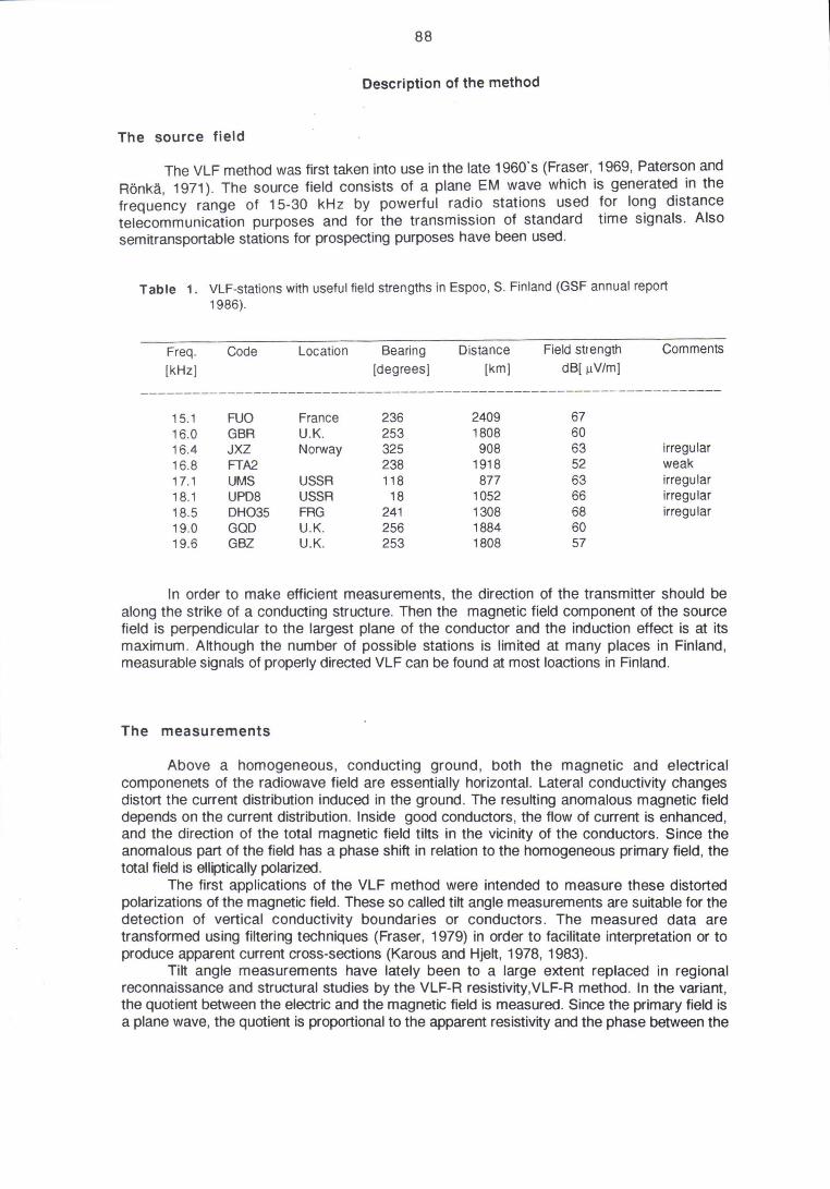
The VLF method was first taken into use in the late 1960's (Fraser, 1969, Paterson and Rönkä, 1971). The source field consists of a plane EM wave which is generate~ in the frequency range of 15-30 kHz by powerful radio stations used f?r lo~g dlstance telecommunication purposes and for the transmission of standard time Signals. Also semitransportable stations for prospecting purposes have been used.

Table 1. VLF-stations with useful field strengths in Espoo, S. Finland (GSF annual report 1986).

Freq . Code Location Bearing Distance Field strength Comments

[kHz] [degrees] [km] dB[ IlV/m]

- - ------- - - - ----------------------- ------------------ -------- ------

15.1 FUO France 236 2409 67 16.0 GBR U.K. 253 1808 60 16.4 JXZ Norway 325 908 63 irregular 16.8 FTA2 238 1918 52 weak 17.1 UMS USSR 118 877 63 irregular 18.1 UPD8 USSR 18 1052 66 irregular 18.5 DH035 FRG 241 1308 68 irregular 19.0 GQD U.K. 256 1884 60 19.6 GBZ U.K. 253 1808 57

In order to make efficient measurements, the direction of the transmitter should be along the strike of a conducting structure. Then the magnetic field component of the source field is perpendicular to the largest plane of the conductor and the induction effect is at its maximum . Although the number of possible stations is limited at many places in Finland, measurable signals of properly directed VLF can be found at most loactions in Finland.

The measurements

Above a homogeneous, conducting ground, both the magnetic and electrical componenets of the radiowave field are essentially horizontal. Lateral conductivity changes distort the current distribution induced in the ground. The resulting anomalous magnetic field depends on the current distribution. Inside good conductors, the flow of current is enhanced, and the direction of the total magnetic field tilts in the vicinity of the conductors. Since the anomalous part of the field has a phase shift in relation to the homogeneous primary field, the total field is elliptically polarized.

The first applications of the VLF method were intended to measure these distorted polarizations of the magnetic field. These so called tilt angle measurements are suitable for the detection of vertical conductivity boundaries or conductors . The measured data are transformed using filtering techniques (Fraser, 1979) in order to facilitate interpretation or to produce apparent current cross-sections (Karous and H jelt, 1978, 1983).

Tilt angle measurements have lately been to a large extent replaced in regional reconnaissance and structural studies by the VLF-R resistivitY,VLF-R method. In the variant, the quotient between the electric and the magnetic field is measured. Since the primary field is a plane wave, the quotient is proportional to the apparent resistivity and the phase between the

89

fields (Tikhonov, 1950; Cagniard, 1953).

Pa = (1/wl1) (E/H)2 (1 )

<1> = arg (E/H)

The phase is a very sensitive and useful parameter for determining the conductivities of the bedrock structures.

Equipment

Practically all measurements in Finland are performed with the Canadian Geonics EM16R instrument, one of the main designers (V. Rönkä) of which is Finnish by birth. The magnetic field components are recorded using standard ferrite coils and the electric field using two electrodes positioned 10m apart. Amplification of the signal is provided by circuitry inside the electrode handles. Lately, instrumental development has been going on at the Geological Survey of Finland to produce an airborne variant of the VLF-R system. (GSF Annual Report 1986) .

Interpretation principles

2-layer models, nomogram interpretation

The common procedure in VLF-R interpretation has been to use the 2-layer nomograms provided by the manufacturer of the instrument (Geonics, 1975). As Hjelt et al. (1985) have pointed out, the nomograms are only a graphical counterpart of the classical two-Iayer apparent resistivity of magnetotellurics:

IPal = P1 (coth2 x + tan2 y)/ (1 + coth2 x * tan2 y) (2)

ct>= 2 atan {((coth2 x - 1) + tan y)/ (coth x (1 + tan2 y))}

with x = - y + coth-1 (/ (P2/P1)}

y = - h1 I (1[l1of / A1)

The nomograms provide a rapid means of establishing the main electric parameters of the bedrock. Provided the surface layer conductivity can be estimated (normally from the properties of the soil at the measuring sites) , the thickness of the overburden and the conductivity (resistivity) of the bedrock can be found. Since only two parameters are measured at each site (Pa and <1» , only two model parameters can be found per site. If two perpendicular (or nearly perpendicular) signals are available, additionallayer parameters can be determined (Hjelt et al. , 1985).

2-layer models, computer methods

Since the two-Iayer curves are mathematically quite simple, the nomogram two-Iayer

90

intrepretation can also be performed quicklyon a modest calculator or microcomputer. The most efficient interpretative procedure is to combine the VLF tilt angle and VLF-R measurements as has been pointed out by Kaikkonen (1980b) . 20 modelling requires a numerical calculation program , e.g. of the finite element type (Kaikkonen, 1979, 1980a, 1980b).

Computer 20 modelling

An alternative to 20 interpretation is to calculate apparent current distributions, by e.g. , using the filtering technique proposed by Karous and Hjelt (1978, 1983). In this technique, the current density induced in the ground is assumed to be confined to a layer of preselected thickness Oz. The distribution of the current density in this layer is obtained by the linear filter (Karous and Hjelt, 1983)

!:l.z * 1 (0)/(271") == - 0.102 H-3 + 0.059 H-2 - 0.561 H-1 + 0.561 H1 - 0.059 H2 + 0.102 H3 (3)

1(0) == 0.5 [I (!:l.x /2) + I (- !:l.x /2)]

Repeating the filtering for data sets with various !:l.x, the current density is factually approximated at various depths . The result can be considered as an apparent current distribution (pseudosection) and it is highly illustrative for picturing the qualitative behaviour of the subsurface electrical structure. It is straightforward to produce a similar nonlinear filter and thus to approximate the true current distribution more realistically.

Field examples

VLF-R measurements are often used as a complementary and high-frequency check ("calibration") on AMT soundings, but their greatest value is as such in reconnaissance profiling . The productivity of VLF-R measurements is very good and in highly resistive environments weil conducting zones may be detected from depths of about 200-300 meters. Resistivity work should, whenever feasible, be completed by tilt angle measurements, since these are the most sensitive ones for detecting vertical conductivity contrasts . The use of both versions of the VLF-method is described in the subsequent examples.

The location of contacts between different rock types (Sotkamo, Talvivaara)

This VLF study was carried out jointly in 1981 by the Department of Geophysics, University of Oulu, and the Geological Survey of Finland. The survey area is situated in Sotkamo, in the southern part of the Kainuu schist belt (Fig 1.) Three main profiles were measured in order to study the detectional capabilities of the AMTS and VLF-R methods. One of the measured profiles crossed the contact between two bedrock blocks. The block of mica schists is resistive (typical in situ resistivities being 2000-3000 Om) whereas the block consisting of black schists is a good conductor (typical in situ resistivities being 0.01-10 Om).

The thickness of the overburden is only a few meters. The contact can be located quite accurately, within a few meters, when the H-polarization is measured and when the density of the measuring points along the profile is sufficient (Fig. 2A) . The change in E-polarization curves is more gradual (Fig. 28). For reliable interpretation tests, measurements in different

A)

C)

i o

553

i 1 KM

91

B)

200km,

~ Cl -

Presvecokarelidic 0 Granite complex Ouartzite

Phyllite . black schist

f---f • • ~ D mJ

~ Mica schist

~ Garnet-hornblende

AMT-sounding VLF-R-profile

schist

Ni-Cu- Zn-mineralization

Block schist

Mico schist

Quartzite

5E>rpent inite

558

7099

Fig.1. Location (A) and geology (8) & (C) (Heino and Havola, 1980) of the VLF survey area in Sotkamo, Talvivaara, in the southern part of the Kainuu schistbelt.

92

directions in the survey region are essential to make sure that true H-polarization data are obtained.

B) VLF·R TALVIVAARA. 1981 STATIONJXZ ~~

~:Et ~:s:=:zs:zs:~. ~-?§§~s::;6;~~~d ~~~ ; .

Et;-~~~C: ~- ._+ _ _ 1-_ . +--I-- -+- -I---- - ---- - ..:- -..J

AMT: 9 10 11 12 13 1~ 15 txxxxxxxxxxxxxxxxxxxxxxxxxxxxxxxxxxx

conductlng zone

Fig. 2. VLF-R profiles above the contact between blocks of resistive mica schists and conductive black schists in the Talvivaara area: (A) H-polarization, (8) E-polarization .

VLF-R ~ TALVIVAAAA,.1981

~ STATION FUO

~~I>~~~~z~~~A$§_~.:~6\~v=~:~~§§~,>~~§r9~~:::~~dS~6~S ~~~<1 o 100 200 300 ~OO 500 600 700 800 900 1000 1100 X(M)

..... ~ ~ .c:-:--... ....--=::":>~Z\ ~ ~ I : . '7" ' SO: Zj' ~ : o ~3bO \(0 500 Gi 760 800==;00 1000 1100x(M)

Black schist Mica schist Quartzite Black schist

3-10m--- ~ _ .. 7-15 m ____ -4-10 rn--1. t t ~

resistive area

~

~ -4-10 m-~

15-20 m

Fig. 3. VLF-R H-polarization profiie ac ross the bedrock contact of Fig. 2 and its 2-layer interpretation. At each part ofthe profile the typical range of depths to the conductive bedrock is given in meters. The rocks marked mica sChists based on geological mapping are good conductors, suggesting that the black schist block continuees up to the quartzite area (cf., the text).

93

The interpretational value of the phase angle is demonstrated in Fig. 3 (profile 3 of Fig. 1). The contact between the mica and black schist blocks (at about x = 150 m) is based on geological mapping of the surface rocks with uncertainties resulting trom the overburden. The apparent resistivity is higher above the area mapped as schists. But since the phase is still on a high level, it may be concluded that the mica schist area in fact contains more highly conductive material, i.e., the black schists extend up to the quartzite area. The depth of the surface of the conductors can be determined by the 2-layer nomogram technique. Increasing apparent resistivity values together with a simultaneous low level of the phase angle above the quartzite area shows that no conductors can be detected in this area.

Fig. 4 shows a comparison between the VLF-R data and the interpreted AMT 1 D conductive models for profile 4 in Fig. 1. (For further discussion of the AMTS profiles, see Hjelt et al. , this issue) . In the resistive area (AMT points 8-16) the apparent VLF-resistivity is high and the phase weil below 45°. Indications of conductors can be seen between 260-320 m and 780-860 m on the profile (the apparent VLF-resistivity descreases and the phase is above or close to 45°). Here the AMT-soundings support the conclusions drawn trom the VLF-R data. According to the AMTS interpretation, conductors are located at a depth of 200-300 m. The VLF field does not penetrate deep enough at these sites to give indications about the deeper conductors of the 2D AMT model. Thus the VLF-R can be useful as a reconnaissance tool for locating conductors in resistive regions down to a few hundred meters. It is preferable that the VLF-R results are complemented by either AMTS or DeS results .

VLF·A ~ TAlVIVAAAA. I981

~~I ST"'ON'»<~ ~

g;:~ 7 ~ SY~ :':; 1 260 30

~!I z~ o 1~;:;;: 560

760 :rZ:o ~ooo (.:gq 1100 1200 X(M)

#+fJ 1100 1200 X(M) 700 7=== 800 900 1000

I narrow conductor POSSi~lä- CÖ~ductor

2 3 4 5 10 11 12 13 14 15 16 17 18 19 0 24 25

go .. ---- resistive area ---

x'" -1 • ... • "- • Wo z1 Q~

Fig. 4. Correlation between VLF-R, H-polarization data and interpreted AMT Gonducting layers.

The location of vertical or nearly vertical zones of conductive and resistive veins (Haukipudas, Northern East Bothnian schist areal

The northern East Bothnian schist area represents a typical Finnish bedrock complex. Greywackes and volcanics with layers of graphitic schists containing some (pyrite and pyrrhotite) mineralizations alternate with resistive granitic rocks. The topography is rather flat and the Quaternary overburden is typically 1 to 8 meters thick, and seldam exceeding twenty meters. The bedrock at the sampie profile of the northern East Bothnian schist area is layered and consists of mainly steeply dipping, parallel and thin conducting layers of graphitic schist.

94

A)

B)

C) '-I :

x/m 1000

f"

Fig. 5. Part of a test profile across the northern East Bothnian schist area. A. Ground magnetic vertical anomaly and its 20 interpretation: 1 == calculated anomaly; 2 == measured anomaly; 3 == 20 model with susceptibility in SI units . B. VLF tilt angle and corresponding apparent current density pseudosection: 1 == Re {Hz}; 2 = Im{Hz}; 3 == irel; 4 == 2*irel; 5 == 3*irel. [VLF-station JXZ, 16.4 kHz]. C. VLF-R data: 1 = parallel apparent res istivity [E-pol, JXZ, 16.4 kHz]; 2 = perpendicular apparent resistivity [H-pol, FUO, 15.1 kHz]; 3 = phase (E, H) trom 25 to 400 ; 4 = phase (E, H) trom 50 to 700 ; 3 = phase (E, H) above 700 (trom Hielt, 1979).

95

The sampie profile, only apart of which is shown in Fig. 5, runs across a distinct aeromagnetic anomaly. The corresponding magnetic vertical component ground profile confirms the verticality of the conducting and magnetized structure. Many VLF tilt angle anomalies correlate with the magnetic anomalies. The magnetic anomalous part extends from about x = 700 m to 1.400 m with a clear intern al structure of strongly magnetized veins (Fig. 5A) . The VLF tilt angle profile has anomalies on the order of 15-25 % at both ends of the magnetized region (Fig. 5B). The tilt angle profile can qualitatively be interpreted either as two distinct vertical conductors at about x = 700 and 1400 m or as a broader conductive block of about the same width as the main magnetized region , but with a possible internal structure. The equivalent current density interpretation (bottom part of Fig. 5B) , obtained by the Karous-H jelt filter (Karous and H jelt, 1977, 1983), confirms the verticality of the structure and bears vague evidence in favour of the latter interpretation.

The VLF-R results (Fig. 5C) indicate that the whole structure from x = 700 to 1400 m conducts weil , since both the apparent resistivity is low and the phase angle clearly exceeds 45l:l: . This profile shows definitely that also the conductivity has an internal structure and consists apparently of vertical conductive bands (veins) . As in magnetotellurics , the perRendicular apparent resistivity (H-polarization) delineates the conductors more properly thanthe parallel (E-polarization) data.

Around x = 800 m, an exceptionally small point separation (5, even 2.5, meters) was used. The result demonstrates the horizontal resolution capacity of the VLF-R method in SUC!l

vertically layered conductive regions . (One should recognize that the GEONICS EM16R instrument used is actually insensitive to apparent resistivities below 10 Dm, so all the lower values in Fig. 5C should be considered only qualitatively . Therefore all the phase values are given in three broad categories only.)

Regional structural research (Suhanko intrusion)

A discontinuous belt of layered mafic intrusions extends 270 km across northern Finland trom Tornio, on the Swedish border, to Näränkävaara, at the Soviet bord er (cf. , Fig. 2 in Rekola, 1985). The intrusions of Suhanko and Konttijärvi, belonging to this belt, intruded between the Archean basement cOlTlplex and the Peräpohjola Schist Belt of Svecokarelian metasediments and volcanics about 2.25 Ga ago (Vuorelainen et al. , 1982). The Suhanko intrusion is composed mainly of monotonous gabbro. Discontinuous belts of ultramafic rocks, predominantly peridotite, occur at the marginal zone near the base of the intrusion, in contact with the gneissose granite of the basement. The lower part of the marginal zone has discontinuous layers of pyrrhotite with some Cu-Ni-mineralizations. Some minerals of the platinum group have been found in the Konttijärvi intrusion (Isohanni, 1971 , Vuorelainen et al. , 1982). Geophysical studies of the Niittylampi- Vaaralampi mineralization of the Suhanko intrusion have been described by Rekola (1985).

A project was carried out in 1984-86 by the Department of Geophysics, University of Oulu, in co-operation with the Lapin Malmi Company (Outokumpu Oy) and financed by the Finnish Ministry of Trade and Industry to study and determine the main structure of the Suhanko intrusion. A considerable number of VLF (94 line-km) and AMT measurements (about 500 soundings) were carried out and interpreted during the project (Pernu et al. ,1986; Keränen, 1987; Lerssi,1988). A wealth of other data gathered since 1964 by the Lapin Malmi company (previously Outokumpu Oy) and by the project itself was combined to obtain an integrated structural model for the intrusion.

The western and southeastern wings of the intrusion are wedgelike basins with thicknesses varying trom 100 to 500 m. The conducting layers in the contact between the gabbros of the intrusion and the surrounding granites are clearly to be seen in the VLF-R data. Thus the method can be used to locate the boundary along most parts of these wings. The depth of the intrusion requires lower than VLF trequencies to follow the conducting layers at the contact. The northern wing is thicker and the exact geometry of its boundary cannot be

96

.----------------------------_._--_._------

I , , I

~ \ 'l

~KONTTIJÄRvI -min er. 1~4 Oligoclase granite

c=J Gneissose granite

~ Konglomerate ~

Quartzite , Merkel schistg- 7334

-0 I

Hypoabyssal ~ / Siirros spilites

++++ ++++ d- + + +

+

+ 7334

Metagabro and metadiorite 0'--__ tL-_-"3 km

Ultramafic rocks

Fig. 6. Simplified geological map of the area studied, Suhanko (Isohanni, 1971).

. ",~ ,,' Measured Pa (Qm ) ,,'

" Measured phase <p ( ') " rau

..-/ Bedrock contact from Isohanni ( 1971)

Fig. 7_ Map of VLF-R profiles across the boundaries of the Suhanko intrusion.

,

0--= . > .!. 1 >

i , . ~

1 I .. -: . >

97

o ~ . . 1 > ~

~ Rocks of the layered intrusion

~ Interpreted conductance (5 ) , 2

Bedrock cont acts f rom I s ohanni ( 1971 )

Fig. 8. Electrical structural interpretation of the Suhanko intrusion , based on AMTS and VLF data.

. o ..

determined unambiguously. The central part of the intrusion is about 700-1000 m thick and the western boundary is steep or dips subvertically westwards.

The map of Fig . 7 brings together all the VLF profiles on and around the Suhanko intrusion. The profiles have been classified and summarized into the interpretation map of Fig. 8. The surface conductors can be located and the whole intrusion can be divided into parts based on conductivity . Three categories were used: surface conductors , deep conducting horizons and resistive areas. The surface conductors were situated between the surface and depths trom 200 to 300 m. They occur mainly at the southeastern and southern

7 403333F

98

contacts of the intrusion. The deep conductors are located 300 m or more below the surface. Areas are classified as resistive whenever the apparent resitivity is higher than1 000 Om and the phase angle below 20tx simultaneously. When the resistivity at the surface is high (about 10000 Om) , the VLF-R method can be used to locate conducting horizons down to about 300 m .

When one combines the VLF-R data with the AMTS results, a final electrical interpretation map (Fig. 8) is obtained, clearly indicating the basinlike structure of the intrusion. The gravity and magnetic structural interpretations , which mainly support the electrical models, will not be discussed here further , although they have been essential to arriving at with the final result of Fig. 8.

Other applications

In addition to the foregoing examples ,VLF and VLF-R profiling can and has been applied to a variety of geological problems. The relief of a resistive bedrock can be reliably determined in cases where the thickness of the overburden is a significant part of the skin-depth at VLF trequencies. The conductance of a ground-water layer is the dominating part of the overburden conductance. Since the resistivity of a typical ground-water layer does not vary significantly, the two-Iayer interpretation of VLF-R measurements can provide reasonable estimates of the thickness of the ground-water layer.

The quality of the bedrock can be assessed trom directional information about the ground electrical conductivity/resistivity and its anisotropy. Since the VLF method is essentially a plane wave method, this would require recording of the complete impedance tensor as in magnetotelluric measurements. Whenever two VLF transmitting signals with a difference in bearings trom the transmitters close to 90 degrees are available, such directional surveys can be made. Several factors , such as fracturization, less the resistive minerals and overburden depressions, affect bulk bedrock resistivity in a slmilar manner. This makes interpretation of VLF data ademanding task indeed, which cannot be solved without additional information obtained by other methods. The best result requires - as in any application of geophysics - an intelligent, problem-integrated and professional combination of geophysical and geological data.

References

Cagniard , L. , 1953. Bas ic theory 01 the magnetotelluric method 01 geophysical prospecting. Geophysics18, 605-635.

Fraser, D.C., 1969. Contouring of VLF-EM data. Geophysics 34, 958-967. Geonics Ud., 1975. EM16-R(RADIOHM) . Two-Iayer interpretation curves.Techn . Note TN-1 ., 8 +

14 pp. GSF Annual Report 1986. VLF-stations. (in Finnish). Heino , T. & Havola, M. , 1980. Geology in the Jormasjärvi-Talvivaara area. Report M

19/3344/-80/3/10, Geol. Survey 01 Finland (in Finnish) Hielt, S.-E., 1979. Electromagnetic plane wave methods in prospecting. Proc . 24th International

Geophysical Symposium, 4.-7. Sept., Krakow, 11 pp. Hielt, S.-E ., Kaikkonen, P. & Pietilä , R. , 1985. On the interpretation 01 VLF resistivity

measurements. Geoexploration: 23, 17-181. Isohanni, M., 1971. The bedrock of the Palovaara-Suhanko area in the southeastern part of the

Peräpohja schist zone (in Finnish). M. Sc. thesis, Dept. 01 Geology, Univ. of Oulu, 127 pp. Karous , M. & Hielt, S.-E., 1978. Determination of apparent current density from VLF

measurements . Dept. 01 Geophysics, Univ. 01 OUlu, Contrib. 89, 18 pp. Karous , M. & Hielt, S.-E. , 1983. Linear 1i1tering 01 VLF dip-angle measurements. Geophys.

Prospecting 31, 782-794.

99

Kaikkonen , P., 1979. Numerical VLF modeling. Geophys. Prospecting 27 , 815-834. Kaikkonen, P., 1980a. Numerical VLF, VLF-R and AMT profiles over some complicated models.

Acta Univ. Oul. : A 91 , 1980, Phys.16, 34 pp. Kaikkonen , P. , 1980b. Interpretation nomograms for VLF measurements. Acta Un iv. Oul. : A 92 ,

1980, PhYS.17, 48 pp. Keränen, T., 1986. A study of the structure of the Suhanko layered intrusion by using the AMT and

the VLF-R methods. (in Finnish) M. Sc. thesis , Dept. of Geophysics, Univ. of Oulu, 71 + I pp. LerSSi, J ., 1986. A study of the structure of the Suhanko layered intrusion by using the gravity and

magnetic methods (in Finnish). M. Sc. thesis, Dept. of Geophysics, Univ. of Oulu, 77 + VIII pp. Paterson, N.R. & Rönkä, V. , 1971. Five years of surveying wi th the Very Low Frequency­

Electromagnetic method. Geoexploration : 9, 7-26. Pernu , T. , Keränen, T. , Lerssi, J ., & Hjelt, S.-E. , 1986. The geophysica l structural study

of the Suhanko layered intrusion. (in Finn ish). Final project report, Dept. of Geophysics , Un iv. of Oulu , 44 pp.

Rekola, T. , 1985. Results of electrical and electromagnetic measurements in Vaaralampi-N iittylampi, Ranua. In L. ESkola, A. Phokin (eds): Electrical prospecting for deposits in the Baltic Shield, part 1: Galvanic methods. Geol. Survey of Finland, Report of Investigations 73, 73-84.

Tikhonov, A.N ., 1950. Onpe.lle"eHHe s" eKTpHCe qKHX x apaKTepHcTHK r"hl6oKHX q"OeB SeMHO)l( KOpB: . .2l0K" . AKa.ll . HahlK CCCP: 73, 295-297.

Vuorelainen , Y., Häkli , A ., Hänninen , E., Papunen , H. , Reini , J. & Törnroos , R. , 1982. Isomerteite and other platinum-group minerals from the Konttijärvi mafic intrusion , Northern Finland. Economic Geology 77, 1511 -1518.