Excess Demand, Supplier-Induced Demand

in Social Health Insurance:

Evidence from China

1. Introduction

China has undergone one of the most drastic reforms of social health

insurance, beginning in 2009. Now, Urban Employee Basic Medical

Insurance (UEBMI), Urban Residents Basic Medical Insurance (URBMI),

and the New Rural Cooperative Medical System (NRCMS) constitute the

basic medical insurance system in China. The reform particularly aims at

increasing coverage and controlling medical expenditure. Since 2009,

social health insurance has covered everyone, urban and rural (Human

Resources and Social Security Development Statistics Bulletin, 2013).

Medical supplies have also shown a slight but steady growth trend.

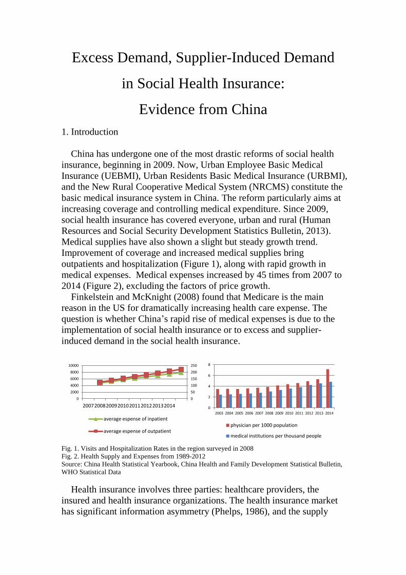
Improvement of coverage and increased medical supplies bring

outpatients and hospitalization (Figure 1), along with rapid growth in

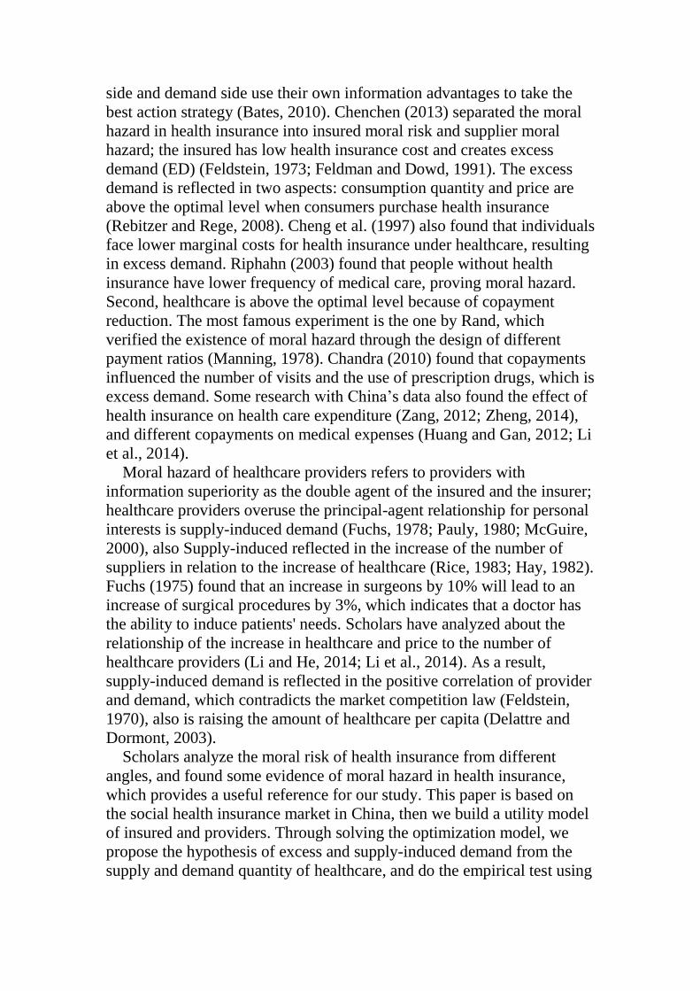
medical expenses. Medical expenses increased by 45 times from 2007 to

2014 (Figure 2), excluding the factors of price growth.

Finkelstein and McKnight (2008) found that Medicare is the main

reason in the US for dramatically increasing health care expense. The

question is whether China’s rapid rise of medical expenses is due to the

implementation of social health insurance or to excess and supplier-

induced demand in the social health insurance.

Fig. 1. Visits and Hospitalization Rates in the region surveyed in 2008

Fig. 2. Health Supply and Expenses from 1989-2012

Source: China Health Statistical Yearbook, China Health and Family Development Statistical Bulletin,

WHO Statistical Data

Health insurance involves three parties: healthcare providers, the

insured and health insurance organizations. The health insurance market

has significant information asymmetry (Phelps, 1986), and the supply

0

50

100

150

200

250

0

2000

4000

6000

8000

10000

2007 2008 2009 2010 2011 2012 2013 2014

average espense of inpatient average espense of outpatient

0

2

4

6

8

2003 2004 2005 2006 2007 2008 2009 2010 2011 2012 2013 2014

physician per 1000 population

medical institutions per thousand people

side and demand side use their own information advantages to take the

best action strategy (Bates, 2010). Chenchen (2013) separated the moral

hazard in health insurance into insured moral risk and supplier moral

hazard; the insured has low health insurance cost and creates excess

demand (ED) (Feldstein, 1973; Feldman and Dowd, 1991). The excess

demand is reflected in two aspects: consumption quantity and price are

above the optimal level when consumers purchase health insurance

(Rebitzer and Rege, 2008). Cheng et al. (1997) also found that individuals

face lower marginal costs for health insurance under healthcare, resulting

in excess demand. Riphahn (2003) found that people without health

insurance have lower frequency of medical care, proving moral hazard.

Second, healthcare is above the optimal level because of copayment

reduction. The most famous experiment is the one by Rand, which

verified the existence of moral hazard through the design of different

payment ratios (Manning, 1978). Chandra (2010) found that copayments

influenced the number of visits and the use of prescription drugs, which is

excess demand. Some research with China’s data also found the effect of

health insurance on health care expenditure (Zang, 2012; Zheng, 2014),

and different copayments on medical expenses (Huang and Gan, 2012; Li

et al., 2014).

Moral hazard of healthcare providers refers to providers with

information superiority as the double agent of the insured and the insurer;

healthcare providers overuse the principal-agent relationship for personal

interests is supply-induced demand (Fuchs, 1978; Pauly, 1980; McGuire,

2000), also Supply-induced reflected in the increase of the number of

suppliers in relation to the increase of healthcare (Rice, 1983; Hay, 1982).

Fuchs (1975) found that an increase in surgeons by 10% will lead to an

increase of surgical procedures by 3%, which indicates that a doctor has

the ability to induce patients' needs. Scholars have analyzed about the

relationship of the increase in healthcare and price to the number of

healthcare providers (Li and He, 2014; Li et al., 2014). As a result,

supply-induced demand is reflected in the positive correlation of provider

and demand, which contradicts the market competition law (Feldstein,

1970), also is raising the amount of healthcare per capita (Delattre and

Dormont, 2003).

Scholars analyze the moral risk of health insurance from different

angles, and found some evidence of moral hazard in health insurance,

which provides a useful reference for our study. This paper is based on

the social health insurance market in China, then we build a utility model

of insured and providers. Through solving the optimization model, we

propose the hypothesis of excess and supply-induced demand from the

supply and demand quantity of healthcare, and do the empirical test using

data from the China Health and Nutrition Survey (CHNS). We also give

some suggestions for China's social health insurance reform.

First, we test excess and supply-induced demand from the perspective

of demand and supply variables, using different variables in the same

model, and including the four part model; Second, we set different

characteristic variables of health insurance according to the different

types of social health insurance in China, which is compared with dummy

variables in the existing literature. Third, we distinguish the excess

demand and release of demand in medical expenditure, and also

distinguish induced supply and accessibility effect, which make our

conclusions more robust.

This paper is organized as follows: The next section introduces the

theory model and analysis. Section 3 is the data, variables and empirical

model design. Section 4 is the empirical test and analysis. Section 4 is the

conclusion and policy suggestions.

2. The Model and Theoretical Analysis

We built a social health insurance model, composed of three party,

social health insurance organization, insured and healthcare providers.

We refer to a health demand model by Grossman (1972) and a supplier-

induced model by Ellis and McGuire (1986).

China’s government provides social health insurance to most of

residents, so we do not consider adverse selection.

The insured are rational and homogeneous except for the likelihood of

illness. The insured's income are Y; the number of healthcare providers

are q; the system includes j healthcare providers; r is the price of

healthcare and exogenous; healthcare providers can decide the number of

healthcare, not the price of healthcare.

The utility function of insured is continuous, differentiable, increasing

and strictly concave, namely 'U > 0， '' 0U , which can ensure insured is

risk averse; the probability of illness is . The utility function of

healthcare providers is V, and ' 0V ， '' 0V .

The insurance contract is ( , )p , is the copayment of social health

insurance, p is the premium.

Final wealth of the insured amounts to1W Y p rq rq in the illness

state and 1W Y p in the health state. The risk utility function therefore

reads: ( ) ( ) (1 ) ( )EU w U Y p rq rq U Y p

Health care providers are concerned about the profits and the patients’

benefits. The utility function therefore reads:

1

( ) ( ) + ( )EV q V rq c q V B qj

with ( )c q denoting the cost of health care providers， 1( )rq c q

j

denoting the profits of a single healthcare provider, ( )B q denoting the

patient's benefit function.

The rational choice of the insured is to maximize their own utility.

max ( ) ( ) (1 )( )EU W U Y p rq rq Y p (3)

To find the solution of maximizing the expected utility function, we

establish Lagrange function:

The first-order condition for the optimum value of p is given by:

'

1 ( ) 0dEU

U r rdq

（4）

With '

1U denoting the marginal utility of risky wealth in the illness

state. A solution * *( )q q implicitly defines the quantity of healthcare as

a function of . In order to obtain additional information about this

function, comparative statics analysis will be performed. It consists in

subjecting the optimum condition (4) to an exogenous shock d . This

will entail an optimal adjustment *dp , resulting in the objective function

EU attaining its maximum somewhere else. However, the new maximum

still must satisfy the condition 0dEU dq . Therefore, the equality to zero

must hold before and after adjustment, resulting in the comparative-static

equation. 2 2

2+ 0

EU EUdq d

q q

(5)

The second term on the left-hand side shows the impact of the shock

on expected utility, and the first term, the impact of the induced

adjustment of q. This can be solved to obtain: 2

2 2

dq EU q

d EU q

（6）

Since '' 0U is regularly assumed, the denominator is negative

( 2 2 0EU q , amounting to the sufficient condition for a maximum).

Therefore, the sign of the numerator determines the sign ofdq

d.

Differentiating (3) w.r.t. q，one obtains 2 ' ''

1 1= ( 1)EU q U r rU rq （6）

'

1 0U ， ''

1 0U , and 0 1 , so（6）>0, then

0dq

d

Conclusion 1: Copayment will affect healthcare consumption of the

insured. The more , the more healthcare demand from the insured.

From the perspective of healthcare providers, the price of healthcare is

constrained by the government, so healthcare providers cannot feel free to

set the price. But healthcare providers have the ability to influence the

quantity q. Healthcare providers maximize their utility (Stano, 1987):

maxq

EV

（6）

The first-order condition for the optimum value of p is given by,

' ' ' '

1 2

1( ) ( ) 0

dEVV r c q V B q

dq j

（7）

' ' ' '

1 2( ) ( )r

c q V V B qj

（8）

With ' '

1( )r

c q Vj

denoting the marginal utility from marginal profit,

which can be a marginal benefit of supply-induced demand. ' '

2 ( )V B q

denoting marginal benefit for the insured from healthcare, which can be

marginal cost, including the time cost of persuading people to buy more

healthcare and the healthcare providers’ psychological cost (Cromwell

and Mitchell, 1986). The healthcare provider may balance the marginal

profit and the insured's benefit. When the marginal profit is equal to the

marginal benefit of the insured, healthcare provider will maximize his

utility.

A solution * *( )q q j implicitly defines the quantity for healthcare as a

function of j. In order to obtain additional information about this function,

comparative statistics analysis will be performed. It consists in subjecting

the optimum condition (7) to an exogenous shock dj . This will entail an

optimal adjustment *dp , resulting in the objective function EV attaining

its maximum somewhere else. However, the new maximum still must

satisfy the condition 0dEV dq . Therefore, the equality to zero must

hold before and after adjustment, resulting in the comparative-static

equation. 2 2

2+ 0

EV EVdq dj

q q j

（9）

The second term on the left hand side shows the impact of the shock on

expected utility, and the first term, the impact of the induced adjustment

of q. This can be solved to obtain:

2

2 2

dq EV q j

dj EV q

（10）

Since '' 0V is regularly assumed, the denominator is negative

( 2 2 0EU q , amounting to the sufficient condition for a maximum).

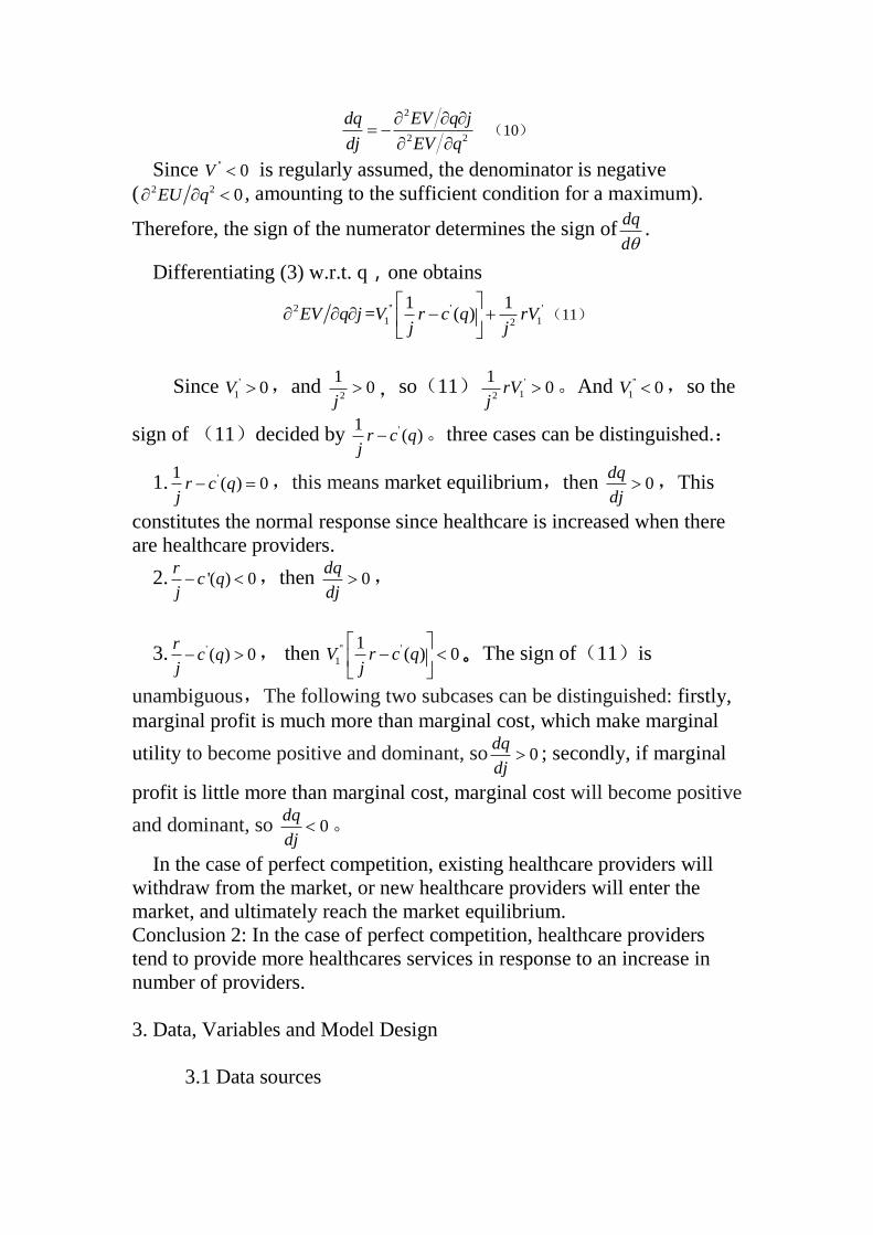
Therefore, the sign of the numerator determines the sign ofdq

d.

Differentiating (3) w.r.t. q，one obtains

2 '' ' '

1 12

1 1= ( )EV q j V r c q rV

j j

（11）

Since '

1 0V ，and 2

10

j ，so（11） '

12

10rV

j 。And ''

1 0V ，so the

sign of （11）decided by '1( )r c q

j 。three cases can be distinguished.：

1. '1( ) 0r c q

j ，this means market equilibrium，then 0

dq

dj ，This

constitutes the normal response since healthcare is increased when there

are healthcare providers.

2. '( ) 0r

c qj ，then 0

dq

dj ，

3. '( ) 0r

c qj ， then '' '

1

1( ) 0V r c q

j

。The sign of（11）is

unambiguous，The following two subcases can be distinguished: firstly,

marginal profit is much more than marginal cost, which make marginal

utility to become positive and dominant, so 0dq

dj ; secondly, if marginal

profit is little more than marginal cost, marginal cost will become positive

and dominant, so

0dq

dj 。

In the case of perfect competition, existing healthcare providers will

withdraw from the market, or new healthcare providers will enter the

market, and ultimately reach the market equilibrium.

Conclusion 2: In the case of perfect competition, healthcare providers

tend to provide more healthcares services in response to an increase in

number of providers.

3. Data, Variables and Model Design

3.1 Data sources

Our data comes from the “China Health and Nutrition Survey Database

(CHNS)” from 1989 to 2011, which covers 12 provinces and nine years.

Among them, the "healthcares" sub-database consists of 113446 samples,

in association with the "personal information" sub database, and

"education" and "work" sub database data; all the data is the original

sample.

In order to observe the behavior of the sample, we used the following

principles of sample selection: excluding samples under the the age of 18;

excluding samples where the description of a person’s health and medical

expenditure were missing; excluding samples who purchased commercial

insurance; deleting samples with other missing observed variables;

removing the samples with some abnormal values. Finally, we got 10018

observations.

3.2 Variables

Our dependent variables are medical expenditure, outpatient

expenditure and inpatient expenditure in answer to, “Are you sick or

injured in the past or how much money has been spent”, “Outpatient

expenditure” and “Inpatient expenditure”. We use these variables to

measure consumption.

According to the previous theoretical analysis, the moral risk of health

insurance includes excess demand and supply-induced demand, which

were reflected in the medical consumption increasing with copayment

decreasing, and medical consumption increasing with the number of

medical institutions increasing. We designed variables from the demand

and supply aspects. Variables about excess demand are outpatient and

inpatient copayment, and variables about supply-induced demand are the

number of health institutions per one hundred thousand of the population

of different regions and health providers per thousand population.

Because there are different types of social health insurance in China, we

designed four characteristic variables according to the answer to the

question of "the type of health insurance".

Our model also includes a series of control variables which influence

medical expenditure. Injury and illness or severity are the main factors;

also individual characteristics variables, so the status of the individual

characteristics such as age, sex, ethnicity, education level, marital status,

urban or rural area, job control variables; and area and time dummy

variables. Table 1. Variables Description

variables type description

Expenditure continuous TREATMENT COSTS

Outpatient continuous OUTPATIENT costs

Inpatient continuous INPATIENT costs

Insurance dummy DO YOU HAVE MEDICAL INSURANCE?

Covered% continuous % OF COST COVERED BY INSURANCE

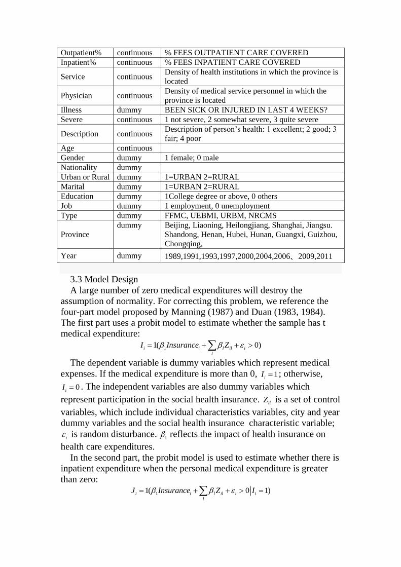
Outpatient% continuous % FEES OUTPATIENT CARE COVERED

Inpatient% continuous % FEES INPATIENT CARE COVERED

Service continuous Density of health institutions in which the province is

located

Physician continuous Density of medical service personnel in which the

province is located

Illness dummy BEEN SICK OR INJURED IN LAST 4 WEEKS?

Severe continuous 1 not severe, 2 somewhat severe, 3 quite severe

Description continuous Description of person’s health: 1 excellent; 2 good; 3

fair; 4 poor

Age continuous

Gender dummy 1 female; 0 male

Nationality dummy

Urban or Rural dummy 1=URBAN 2=RURAL

Marital dummy 1=URBAN 2=RURAL

Education dummy 1College degree or above, 0 others

Job dummy 1 employment, 0 unemployment

Type dummy FFMC, UEBMI, URBM, NRCMS

Province

dummy Beijing, Liaoning, Heilongjiang, Shanghai, Jiangsu.

Shandong, Henan, Hubei, Hunan, Guangxi, Guizhou,

Chongqing,

Year dummy 1989,1991,1993,1997,2000,2004,2006、2009,2011

3.3 Model Design

A large number of zero medical expenditures will destroy the

assumption of normality. For correcting this problem, we reference the

four-part model proposed by Manning (1987) and Duan (1983, 1984).

The first part uses a probit model to estimate whether the sample has t

medical expenditure:

11( 0)i i l il i

l

I Insurance Z

The dependent variable is dummy variables which represent medical

expenses. If the medical expenditure is more than 0, 1iI ; otherwise,

0iI . The independent variables are also dummy variables which

represent participation in the social health insurance. ilZ is a set of control

variables, which include individual characteristics variables, city and year

dummy variables and the social health insurance characteristic variable;

i is random disturbance. 1 reflects the impact of health insurance on

health care expenditures.

In the second part, the probit model is used to estimate whether there is

inpatient expenditure when the personal medical expenditure is greater

than zero:

11( 0 1)i i l il i i

l

InsuranceJ Z I

The dependent variable is dummy variables which representative of

inpatient medical expenses, and if inpatient expenses are more than 0,

1iJ ; otherwise, 0iJ . The independent variables are dummy variables

which representative of participate in the social health insurance. ilZ is a

set of control variables which include individual characteristics variables,

city and year dummy variables and the social health insurance

characteristic variable; i is random disturbance. 1 reflects the impact of

health insurance on health care expenditures.

In the third and fourth part, the linear model is used to describe the

positive outpatient expenditure and inpatient expenditure:

1log( 1) / log( 1 %)oi i oi i i j ij k ik l il i

j k l

E D I Outpatient Demand SupplyI Z

1 %log( 1) / log( 1)ii i ii i i j ij k ik l il i

j k l

E J D J Inpatient Demand Supply Z

The dependent variable of equation 3 is the logarithm of outpatient

medical expenditure. The dependent variables of equation 4 are the

logarithm of inpatient medical expenses. The independent variables

include demand ijDemand and supply variables ikSupply . ikSupply reflects the

demand for outpatient medical expenditures and inpatient medical

expenditures. k reflects the supply for outpatient medical expenditures

and inpatient medical expenditures. i is random disturbance. ( , ) 0i iCov .

3.4. Empirical Test

(1) Data Description

Sample distribution and characteristics

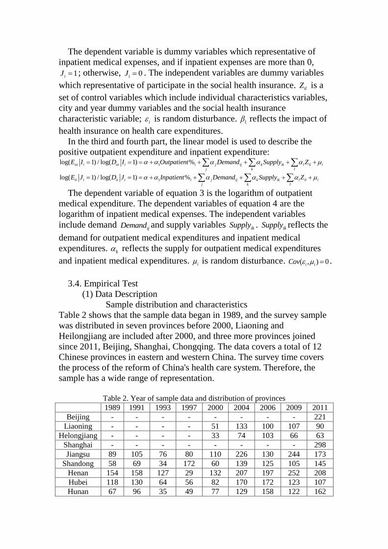
Table 2 shows that the sample data began in 1989, and the survey sample

was distributed in seven provinces before 2000, Liaoning and

Heilongjiang are included after 2000, and three more provinces joined

since 2011, Beijing, Shanghai, Chongqing. The data covers a total of 12

Chinese provinces in eastern and western China. The survey time covers

the process of the reform of China's health care system. Therefore, the

sample has a wide range of representation.

Table 2. Year of sample data and distribution of provinces

1989 1991 1993 1997 2000 2004 2006 2009 2011

Beijing - - - - - - - - 221

Liaoning - - - - 51 133 100 107 90

Helongjiang - - - - 33 74 103 66 63

Shanghai - - - - - - - - 298

Jiangsu 89 105 76 80 110 226 130 244 173

Shandong 58 69 34 172 60 139 125 105 145

Henan 154 158 127 29 132 207 197 252 208

Hubei 118 130 64 56 82 170 172 123 107

Hunan 67 96 35 49 77 129 158 122 162

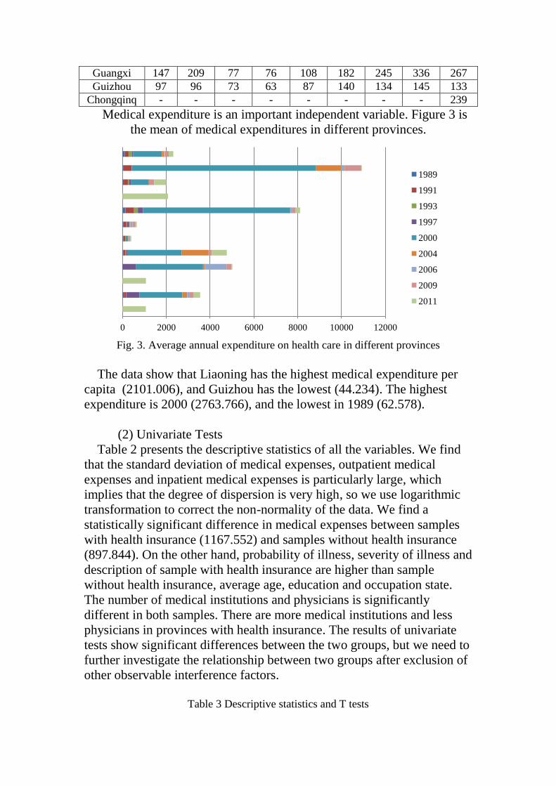
Guangxi 147 209 77 76 108 182 245 336 267

Guizhou 97 96 73 63 87 140 134 145 133

Chongqinq - - - - - - - - 239

Medical expenditure is an important independent variable. Figure 3 is

the mean of medical expenditures in different provinces.

Fig. 3. Average annual expenditure on health care in different provinces

The data show that Liaoning has the highest medical expenditure per

capita (2101.006), and Guizhou has the lowest (44.234). The highest

expenditure is 2000 (2763.766), and the lowest in 1989 (62.578).

(2) Univariate Tests

Table 2 presents the descriptive statistics of all the variables. We find

that the standard deviation of medical expenses, outpatient medical

expenses and inpatient medical expenses is particularly large, which

implies that the degree of dispersion is very high, so we use logarithmic

transformation to correct the non-normality of the data. We find a

statistically significant difference in medical expenses between samples

with health insurance (1167.552) and samples without health insurance

(897.844). On the other hand, probability of illness, severity of illness and

description of sample with health insurance are higher than sample

without health insurance, average age, education and occupation state.

The number of medical institutions and physicians is significantly

different in both samples. There are more medical institutions and less

physicians in provinces with health insurance. The results of univariate

tests show significant differences between the two groups, but we need to

further investigate the relationship between two groups after exclusion of

other observable interference factors.

Table 3 Descriptive statistics and T tests

0 2000 4000 6000 8000 10000 12000

1989

1991

1993

1997

2000

2004

2006

2009

2011

All

N=10018

Insurance=1

N=4637

（1）

Insurance=0

N=5381

（2） Difference

(3)=(1)-(2)

p-

value

95% Confidence Interval of the

Difference

Lower Lower

Variable Mean Std.

Dev Mean

Std.

Dev Mean

Std.

Dev

Expenditure 968.054 401.584 1167.55 470.462 897.844 374.225 269.708*** 0.003 98.291 476.490

Expenditure

0 978.993 403.878 1178.84 472.734 908.505 376.088 270.338*** 0.002 73.287 395.183

Outpatient 0 46.435 586.046 46.435 586.046 0 0 46.435 - - -

Inpatient 0 2829.7 859.399 2829.7 859.399 0 0 2829.7 - - -

Covered% 63.404 37.390 63.404 37.390 0 0 63.404 - - -

Outpatient% 18.801 36.541 18.801 36.541 0 0 18.801 - - -

Inpatient% 22.639 38.535 14.599 30.445 0 0 14.599 - - -

Illness 0.841 0.438 0.816 0.556 0.850 0.384 -0.034** 0.026 -0.072 -0.036

Severe 1.757 0.672 1.739 0.637 1.763 0.683 -0.024** 0.039 0.050 0.103

Description 0.024 0.154 0.866 1.210 1.685 1.248 -0.819** 0.032 -0.810 -0.714

Age 1.290 1.296 58.042 35.364 58.114 56.793 -0.072 0.906 -2.046 1.814

Gender 58.079 47.662 1.530 0.499 1.563 0.496 -0.033 0.213 -0.049 -0.010

Nationality 1.547 0.498 1.710 2.939 2.031 3.403 -0.321 0.143 -0.418 -0.165

Urban or

Rural 1.876 3.192 1.510 0.500 1.721 0.449 -0.211*** 0.000 -0.208 -0.171

Marital 1.619 0.486 0.735 0.441 0.675 0.469 0.06* 0.063 0.043 0.079

Education 0.704 0.457 0.578 0.494 0.808 0.394 -0.23** 0.037 -0.224 -0.190

Job 0.697 0.460 0.535 0.499 0.678 0.467 -0.143** 0.043 -0.150 -0.113

Service 7.570 1.667 7.187 1.847 7.927 1.388 -0.74*** 0.000 -0.767 -0.641

Physician 4.619 2.164 5.237 2.851 4.042 0.880 1.195*** 0.000 0.905 1.050

Note: * imply 10% significant level, ** imply 5% significant level, *** imply 1% significant level

(3) Basic Results

The 4409 samples of the 10018 sample have medical expenses within

four weeks. Table 4 is the result of four parts, and the first two columns

the probit estimates of equation (9); columns 3 and 4 are probit estimates

of equation (10); columns 5 and 6 are OLS estimates of equation (10); the

last two columns are OLS estimation of equation (11). Table 4 Four part test

(1) (2) (3) (4)

B Sig. B Sig. B Sig. B Sig.

constant 0.939*** 0.000 0.939*** 0.000 2.036*** 0.000 -0.044 0.694

Insuranc

e 0.001 0.101 0.012 0.131 0.444*** 0.000 0.622* 0.089

Covered

% 0.101** 0.012 0.146** 0.027

Outpatie

nt% 0.119*** 0.000

Inpatien

t% 0.128* 0.090

Service 0.075 0.246 0.045 0.342 0.104*** 0.000 0.005** 0.038

Physicia

n 0.001 0.128 0.001 0.128 0.090*** 0.000 0.002** 0.018

Illness 0.011*** 0.000 0.013*** 0.000 -0.241*** 0.000 0.116*** 0.000

Severe 0.007*** 0.000 0.013*** 0.000 0.729*** 0.000 0.190*** 0.000

Age 0.021 0.540 0.021 0.540 0.041** 0.032 0.000 0.290

Gender 0.004* 0.092 0.006* 0.092 -0.013 0.299 -0.032 0.212

National

ity 0.015 0.637 0.000 0.343 0.032*** 0.000 0.005** 0.033

Urban

or Rural 0.006** 0.028 0.005** 0.046 0.287*** 0.000 0.072*** 0.008

Marital 0.001 0.172 0.001 0.137 0.570*** 0.000 0.068** 0.040

Educato

n -0.002 0.107 -0.002 0.153 -0.518*** 0.000 -0.150*** 0.000

Job 0.001 0.193 0.001 0.174 0.190*** 0.003 0.105*** 0.001

Type included included included included

Provinc

e

included

included

included

included

Year included included included included

R2 0.217 0.483 0.479 0.322

Adjuste

d R2

0.163 0.372 0.416 0.320

Note: * imply 10% significant level, ** imply 5% significant level, *** imply 1% significant level

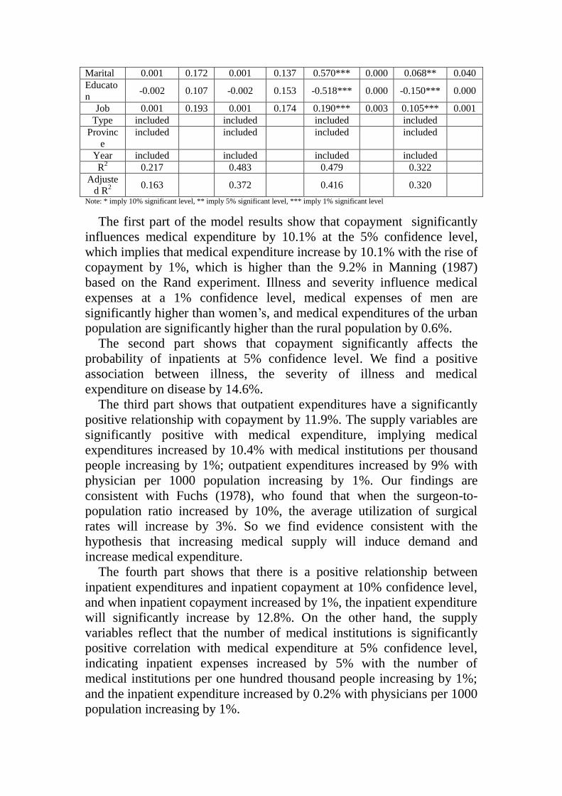
The first part of the model results show that copayment significantly

influences medical expenditure by 10.1% at the 5% confidence level,

which implies that medical expenditure increase by 10.1% with the rise of

copayment by 1%, which is higher than the 9.2% in Manning (1987)

based on the Rand experiment. Illness and severity influence medical

expenses at a 1% confidence level, medical expenses of men are

significantly higher than women’s, and medical expenditures of the urban

population are significantly higher than the rural population by 0.6%.

The second part shows that copayment significantly affects the

probability of inpatients at 5% confidence level. We find a positive

association between illness, the severity of illness and medical

expenditure on disease by 14.6%.

The third part shows that outpatient expenditures have a significantly

positive relationship with copayment by 11.9%. The supply variables are

significantly positive with medical expenditure, implying medical

expenditures increased by 10.4% with medical institutions per thousand

people increasing by 1%; outpatient expenditures increased by 9% with

physician per 1000 population increasing by 1%. Our findings are

consistent with Fuchs (1978), who found that when the surgeon-to-

population ratio increased by 10%, the average utilization of surgical

rates will increase by 3%. So we find evidence consistent with the

hypothesis that increasing medical supply will induce demand and

increase medical expenditure.

The fourth part shows that there is a positive relationship between

inpatient expenditures and inpatient copayment at 10% confidence level,

and when inpatient copayment increased by 1%, the inpatient expenditure

will significantly increase by 12.8%. On the other hand, the supply

variables reflect that the number of medical institutions is significantly

positive correlation with medical expenditure at 5% confidence level,

indicating inpatient expenses increased by 5% with the number of

medical institutions per one hundred thousand people increasing by 1%;

and the inpatient expenditure increased by 0.2% with physicians per 1000

population increasing by 1%.

Most of the control variables are statistically significant and have the

expected sign. Illness and severity of illness influence outpatient and

inpatient medical expenditure at 1% and 5% confidence level. In

common sense, illness samples and serious illness samples should have

more medical expenditure. Age has significant effect on outpatient

expenditures, the older sample has greater expenditure, which is

consistent with previous research. Nations have a significant impact on

outpatient and inpatient medical expenses, which may be affected by the

different characteristics of different nationalities. Rural or urban affected

outpatient and inpatient medical expenditure accounts under at 1%

confidence level, and the urban sample has more outpatient medical

expense (28.7%) and more inpatient expenditure (7.2%) relative to rural

samples, which may be due to medical accessibility. Marital status has a

significant influence on outpatient and inpatient medical expenditure, and

the married sample’s outpatient medical expenses is 57% higher than

unmarried sample’s, and inpatient expenditure is 6.8% higher than

unmarried sample, which may be due to family responsibilities of the

married sample, preferring to avoid the influence on the family brought

by illness, so they consume more healthcares to eliminate the possible

risks. Education degree significantly affected the outpatient and inpatient

medical expenditure at 1% confidence level, compared with the low

education level in the sample, the higher level of education, the lower

outpatient and inpatient medical expense (51.8% and 15% respectively),

which may be due to the high levels sample having more efficient use of

healthcare and can saving the healthcare investment. Job state

significantly affected outpatient and inpatient medical expenses at 1%

confidence level, where samples “with job” have 19% higher outpatient

expense and 10.5% more inpatient expenditure, which may be due to

higher income leading to more medical expenditure.

(4) further Examination of the Conclusion

(i) Further Test of Excessive Demand

The fourth part of the model test shows that health insurance brought

an increase in medical expenses, but it still needs to be tested whether this

increase is due to excessive demand or to the release of medical demand.

Next, we designed a model to test if medical expenses of the insured of

different abilities to pay would ill influence other living expenses, and if

the medical expenditures crowded out the cost of living, implying that

medical expenses are within their pay ability, so if the release of medical

demand is not a major factor, then increase of medical expenditure is

more due to excessive demand.

The model is as follows:

0 1 i l il i

l

iexpense Cov Zered (13)

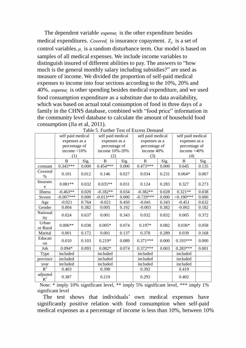
The dependent variable iexpense is the other expenditure besides

medical expenditures. iCovered is insurance copayment. ilZ is a set of

control variables. i is a random disturbance term. Our model is based on

samples of all medical expenses. We include income variables to

distinguish insured of different abilities to pay. The answers to “how

much is the general monthly salary including subsidies?” are used as

measure of income. We divided the proportion of self-paid medical

expenses to income into four sections according to the 10%, 20% and

40%. iexpense is other spending besides medical expenditure, and we used

food consumption expenditure as a substitute due to data availability,

which was based on actual total consumption of food in three days of a

family in the CHNS database, combined with “food price” information in

the community level database to calculate the amount of household food

consumption (Jia et al, 2011). Table 5. Further Test of Excess Demand

self paid medical

expenses as a

percentage of

income <10%

(1)

self paid medical

expenses as a

percentage of

income 10%-20%

(2)

self paid medical

expenses as a

percentage of

income 40%

(3)

self paid medical

expenses as a

percentage of

income >40%

(4)

B Sig. B Sig. B Sig. B Sig.

constant 0.345*** 0.000 0.454*** 0.000 0.473*** 0.000 0.645 0.135

Covered

% 0.101 0.012 0.146 0.027 0.034 0.231 0.064* 0.067

Insuranc

e 0.081** 0.032 0.035** 0.031 0.124 0.283 0.327 0.273

Illness -0.463** 0.020 -0.182** 0.034 -0.382** 0.028 0.321** 0.038

Severe -0.007*** 0.000 -0.013*** 0.000 -0.729*** 0.000 =0.190*** 0.000

Age -0.021 0.764 -0.021 0.450 -0.041 0.343 -0.451 0.632

Gender 0.004 0.382 0.005 0.192 -0.003 0.382 -0.002 0.182

National

ity 0.024 0.637 0.001 0.343 0.032 0.832 0.005 0.372

Urban

or Rural 0.006** 0.038 0.005* 0.074 0.197* 0.082 0.036* 0.058

Marital 0.001 0.172 0.001 0.137 0.378 0.289 0.039 0.168

Educati

on 0.010 0.103 0.219* 0.089 0.371*** 0.000 0.193*** 0.000

Job 0.094* 0.093 0.082* 0.074 0.372*** 0.003 0.283*** 0.001

Type included included included included

province included included included included

year included included included included

R2 0.403 0.398 0.392 0.419

adjusted

R2

0.387 0.219 0.293 0.402

Note: * imply 10% significant level, ** imply 5% significant level, *** imply 1%

significant level

The test shows that individuals’ own medical expenses have

significantly positive relation with food consumption when self-paid

medical expenses as a percentage of income is less than 10%, between 10%

and 20%, between 20% and 40%, at a confidence level of 1%, 5% and 5%

respectively. On the other hand, we do not find significant a relationship

between copayment and food consumption. indicating that the insurance

payments have no significant effect on food consumption, but health

insurance can promote medical spending. We can conclude that it is

because of excessive demand rather than release of medical demand,

because the healthcare is in the ability to afford, so there is no release of

medical demand. Our results are in accordance with Xie Mingming

(2016), who found that health insurance effect on increasing of medical

costs is more ex-post moral hazard factors rather than the release of

medical demand.

When self-paid medical expenses as a percentage of income is above

40%, the insurance copayment ratio has significant positive impact on

food consumption expenditure at 10% confidence level, implying that the

reduction of copayment ratio squeezes food expenditure significantly, and

self-paid medical expenditure has affected the basic life of these

populations, so growth of medical expenditure is more a release of the

demand. At the same time, when self-paid medical expenses as a

percentage of income is above 40%, health insurance has no significant

effect on the increase of medical expenditure, implying that the existing

social health insurance has little effect on the insured when they suffer

from critical illnesses, so government needs to further improve the

security level of the social health insurance for critical illnesses.

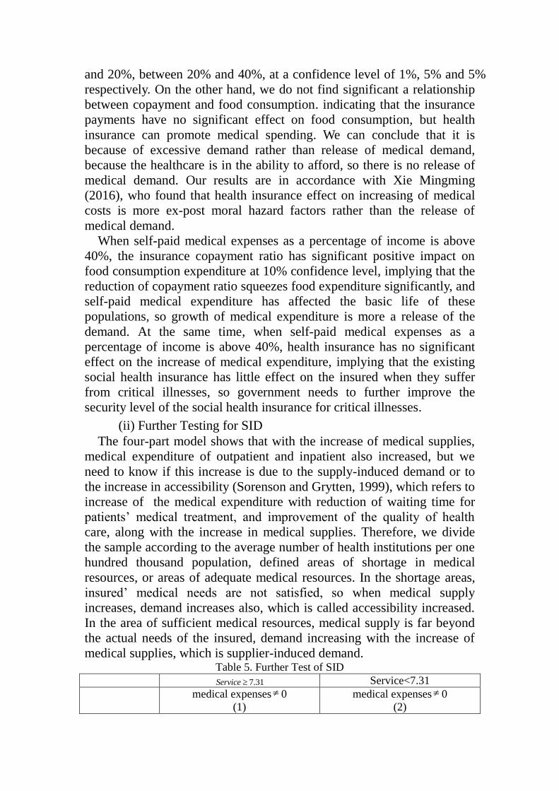
(ii) Further Testing for SID

The four-part model shows that with the increase of medical supplies,

medical expenditure of outpatient and inpatient also increased, but we

need to know if this increase is due to the supply-induced demand or to

the increase in accessibility (Sorenson and Grytten, 1999), which refers to

increase of the medical expenditure with reduction of waiting time for

patients’ medical treatment, and improvement of the quality of health

care, along with the increase in medical supplies. Therefore, we divide

the sample according to the average number of health institutions per one

hundred thousand population, defined areas of shortage in medical

resources, or areas of adequate medical resources. In the shortage areas,

insured’ medical needs are not satisfied, so when medical supply

increases, demand increases also, which is called accessibility increased.

In the area of sufficient medical resources, medical supply is far beyond

the actual needs of the insured, demand increasing with the increase of

medical supplies, which is supplier-induced demand. Table 5. Further Test of SID

7.31Service Service<7.31

medical expenses 0

(1)

medical expenses 0

(2)

B Sig. B Sig.

constant 0.268 0.555 2.855*** 0.000

Insurance 0.451*** 0.000 0.322*** 0.004

Covered% 0.112*** 0.000 0.107*** 0.000

Service 0.263*** 0.000 0.133 0.507

Physician 0.091*** 0.000 0.054* 0.099

Illness -0.189** 0.015 -0.007 0.931

Severe 0.935*** 0.000 0.866*** 0.000

Age 0.001** 0.016 0.001 0.378

Gender 0.002 0.978 -0.118 0.116

Nationality -0.023*** 0.002 0.046 0.167

Urban 0.275*** 0.000 0.529*** 0.000

Marital 0.634*** 0.000 0.583*** 0.000

Education 0.460*** 0.000 0.108 0.333

Job -0.233*** 0.002 -0.451*** 0.000

Type included included

province included included

year included included

R2 0.213 0.117

Adjusted R2 0.212 0.163

Note: * imply 10% significant level, ** imply 5% significant level, *** imply 1%

significant level

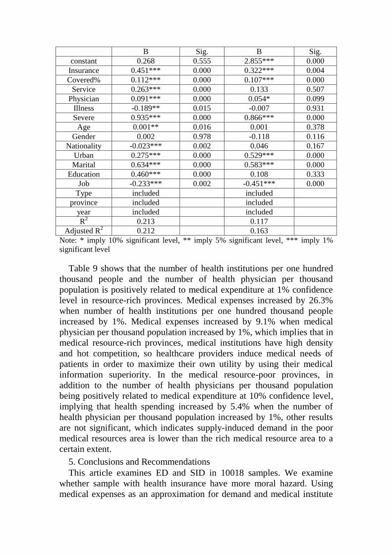
Table 9 shows that the number of health institutions per one hundred

thousand people and the number of health physician per thousand

population is positively related to medical expenditure at 1% confidence

level in resource-rich provinces. Medical expenses increased by 26.3%

when number of health institutions per one hundred thousand people

increased by 1%. Medical expenses increased by 9.1% when medical

physician per thousand population increased by 1%, which implies that in

medical resource-rich provinces, medical institutions have high density

and hot competition, so healthcare providers induce medical needs of

patients in order to maximize their own utility by using their medical

information superiority. In the medical resource-poor provinces, in

addition to the number of health physicians per thousand population

being positively related to medical expenditure at 10% confidence level,

implying that health spending increased by 5.4% when the number of

health physician per thousand population increased by 1%, other results

are not significant, which indicates supply-induced demand in the poor

medical resources area is lower than the rich medical resource area to a

certain extent.

5. Conclusions and Recommendations

This article examines ED and SID in 10018 samples. We examine

whether sample with health insurance have more moral hazard. Using

medical expenses as an approximation for demand and medical institute

as well as physician as an approximation for SID, we find significant

evidence that insurance copayment ratios significantly affect medical

expenditure. Medical expenses increased by 10.1% when health insurance

copayment ratio increased by 1%, the degree for outpatient is 11.9% and

inpatient is 12.8%. Outpatient medical expenditure per capita increased

by 10.4% and inpatient medical expenditure per capita increased by 5%

when health institutions per one hundred thousand increase by 1% per

capita. Outpatient medical expenditure per capita increased by 9% and

inpatient health expenditure per capita increased by 0.2% in relation to

health physician per thousand population increasing.

Further test on excess demand shows that there is excess demand

caused by medical insurance when self-paid medical expenses as a

percentage of income is lower than 40%. While when self-paid medical

expenses as a percentage of income is higher than 40%, the growth in

health spending is more the release of demand. Further test on SID shows

that there is SID in the rich medical resource regions, while accessibility

demand is in the poor medical resource regions.

Our results are consistent with theories and provide some evidence for

further deepening the medical insurance system reform. Firstly, health

insurance copayment has a significant impact on excess demand, so we

should set a reasonable copayment ratio. On the other hand, we find that

excess demand is influenced by the proportion of self-paid medical

expenditure to income, so government should count medical expenses

and compensation degree in different income level populations,

improving the security level of the low income population on the basis of

scientific statistics, in order to release of low income group’s medical

needs and appropriately increase the high income group’s copayment to

control excessive demand.

Secondly, SID has a significant impact on medical expenditure, so we

should affect the supply-induced demand by designing the policy to

influence medical provider's behavior, such as the use of charges (DRGs).

The United States’ inpatient expenses covered by Medicare decreased

from 18.5% to 5.7% and the average inpatient days decreased from 10.4

days to 8.7 days after the implementation of DRG; at the same time you

can see uneven distribution. We also find that uneven distribution of

medical resources in China, the increase of the medical expenditure by

supply of health care in rich medical resource areas are affected by the

supply-induced demand, so the medical insurance reform in China should

proceed from the overall situation, making a reasonable design and

planning for medical resources.

Lastly, medical insurance institutions play an important role in reform.

China's medical insurance institutions have little effect on controlling

medical expenditure, which is mainly due to the low management level of

medical insurance institutions in China, so their information is not

enough. Our government should not only strengthen the construction of

the medical insurance institutions, and realize their information and

deterrent function in the health care market, but also improve the

negotiation mechanism of health insurance. Medical insurance

institutions should explore establishing negotiation mechanisms with the

healthcare providers, to control medical costs.

In short, the social health insurance system originating from third party

payment is the institutional factor of excessive demand and supply-

induced demand. The negative impact of excessive demand and supply-

induced demand reduced to a minimum will improve the social health

insurance system and deepen the reform of the medical system, so that

the basic medical system of China truly achieves the goals of

maintenance and promotion of health of all citizens.

References

[1] Human Resources and Social Security Department, "Human resources and

social security development statistical bulletin", 2013.

[2] Ministry of Health, "2014 China Health Statistical Yearbook", 2015.

[3] Huang Feng, Gan Ni: Moral hazard in medical insurance research, financial

research. 2012, 5.

[4] Gao Chunliang, Mao Feng, Yu Hui. Pay incentive mechanism, financial

burden and Chinese medical security system-based on documents

interpretation of the evolution of medical system. management world, 2009, 4.

[5] Li Ling, Li Ying, Yuan Jia Research and influence of moral hazard in medical

and health reform in China. Chinese health economy, 2014, 1.

[6] Yang Jinxia, Li Shixue. On the new rural cooperative medical institutions

designated medical institutions do not regulate the behavior of regulatory ideas

to explore. China's health economy. 2006, 3.

[7] Yuan, Sun Yuemei, Chen Zhen, "Moral risk" of commercial medical insurance

in China, insurance research, 2014, 6.

[8] Pan Jie, Lei Xiaoyan, Liu Guoen. Does Health Insurance Lead to Better

Health?, economic research, 2013, 4.

[9] Wu and Shen Shuguang: An Empirical Study on the impact of new rural

cooperative medical system on the health of farmers, t insurance research,

2010, 6.

[10] Zang Wenbin, Liu Guoen, Xu Fei, Xiong Xianjun, The Effect of Urban

Resident Basic Medical Insurance on Household Consumption, economic

research, 2012, 6.

[11] Xie Mingming, Wang Meijiao, Xiong Xianjun: "moral hazard or medical

demand release? - medical insurance and medical expenses growth",

insurance research. 2016, 1.

[12] Bates L. J., K. Mukherjee and E. Rexford, Medical Insurance Coverage and

Health Production Efficiency. Journal of Risk and Insurance, Vol.77, No.1,

2010, pp.211-229.

[13] Chandra A., J. Gruber, and R. McKnight, Patient Cost-Sharing and

Hospitalization Offsets in the Elderly. American Economic Review, Vol.100,

No.1, 2010, pp.193-213.

[14] Cheng, S. H., and T. L. Chiang, The Effect of Universal Health Insurance on

Health Care Utilization in Taiwan, Results from a Natural Experiment. Journal

of the American Medical Association, Vol.278, No.2, 1997, pp.89-93.

[15] Cromwell J, J. B. Mitchell. Physician-induced Demand for Surgery. Health

Economics, Vol.5, No.4, 1986, pp.293 -231.

[16] Delattre, E., B. Dormont, Fixed fees and physician-induced demand: A panel

data study on French Physicians. Health Economics. No.12, 2003, pp.41-754.

[17] Duan, N., W. Manning, J. C. Morris, and J. Newhouse. A Comparison of

Alternative Models f or the Demand for Medical Care. Journal of Business and

Economic Statistics, Vol.1, No.2, 1983, pp.115-126.

[18] Ellis A. P. and G. M. Thomas, Provider behavior under prospective

reimbursement: Cost sharing and supply, Journal of Health Economics, Vol.5,

No.2, 1986, pp.129-151.

[19] Evans Robert G. Supplier induced demand: Some empirical evidence and

implications in the economics of health and medical care. London: Macmillian.

1974.

[20] Feldman, R and Dowd, B, A New Estimation of the Welfare Loss of Excess

Health Insurance. American Economic Review, Vol.81, 1991, pp.297-301.

[21] Feldstein, M. S, the Rising Price of Physicians' Services. Review Economic

and Statistics, Vol.52, No.2, 1970, pp.121-133.

[22] Feldstein, M, Welfare Loss of Excess Health Insurance. Journal of Political

Economy, Vol.81, No.2, 1973, pp.251-280.

[23] Finkelstein, A, and R. McKnight, What Did Medicare Do? The Initial Impact

of Medicare on Mortality and Out of Pocket Medical Spending. Journal of

Public Economics, Vol.92, 2008, pp.1644-1668.

[24] Finkelstein, A., S. Tanbman, B. Wright, M. Bernstein, J. Gruber, H. Allen,

and K. Baicker, The Oregon Health Insurance Experiment: Evidence from the

First Year. NBER Working Paper, No. 10365, 2011.

[25] Fuchs V. R., the Supply of Surgeons and the Demand for Operations, NBER

Working Paper, No. 236, 1978.

[26] Grossmna,M, On the concept of health capital and the demand of health.

Political Eocnomy, Vol.80, No.2, 1972, pp.223-255.

[27] Grossman M, the Human Capital Model of the Demand for Health. National

Bureau of Economic Research, No.7078, 1999.

[28] Lei, X. and W. Lin, The New Cooperative Medical Scheme in Rural China:

Does More Coverage Mean More Service and Better Health? Health

Economics, Vol.18, 2009, pp.25-46.

[29] Manning, W., G., Joseph, P. Newhouse, N. Duan, E. B. Keeler and A.

Leibowitz, Health Insurance and the Demand for Medical Care: Evidence from

a Randomized Experiment. American Economic Review, Vol.77, No.3, 1987,

pp.251-277.

[30] Pauly D., M. V. Pauly, Doctors and Their Workshops: Economic Model of

Physician Behavior, University Chicago Press, Chicago, 1980.

[31] Phelps, C. E, Health Economics, Reading, MA: Addison-Wesley, 1986.

[32] Rebitzer J. B, M. Rege, C. Shepard, Influence, Information Overload, and

Information Technology in Health Care. England: Emerald Group Publishing

Limited, 2008.

[33] Sorenson R.J., J. Grytten, Competition and supplier-induced demand in a

health care system with fixed fees. Health Economics, No.8, 1999, pp.497 -

508.

[34] Stano, M., A Clarification of Theories and Evidence on Supplier-Induced

Demand for Physicians' Services, The Journal of Human Resources, Vol.22,

No.4, 1987, pp.611-620.

[35] Wagstaff A., W. Yip, M. Lindelow and C. H. William, China's health system

and its reform: a review of recent studies, Health Economics, Vol.18, No.2,

2009, pp.7-23.