Expedition 314 methods - IODP Publications

Proc. IODP | Volume 314/315/316

Kinoshita, M., Tobin, H., Ashi, J., Kimura, G., Lallemant, S., Screaton, E.J., Curewitz, D., Masago, H., Moe, K.T., and the Expedition 314/315/316 Scientists

Proceedings of the Integrated Ocean Drilling Program, Volume 314/315/316

Expedition 314 methods1

Expedition 314 Scientists2

Chapter contents

Introduction . . . . . . . . . . . . . . . . . . . . . . . . . . . 1

Logging while drilling . . . . . . . . . . . . . . . . . . . . 1

Onboard data flow and quality check . . . . . . . 6

Log characterization and lithologic interpretation . . . . . . . . . . . . . . . . . . . . . . . . . 7

Physical properties . . . . . . . . . . . . . . . . . . . . . . 8

Structural geology and geomechanics . . . . . . . 9

Log-seismic correlation . . . . . . . . . . . . . . . . . . 11

References . . . . . . . . . . . . . . . . . . . . . . . . . . . . 13

Figures . . . . . . . . . . . . . . . . . . . . . . . . . . . . . . . 15

Tables. . . . . . . . . . . . . . . . . . . . . . . . . . . . . . . . 29

1Expedition 314 Scientists, 2009. Expedition 314 methods. In Kinoshita, M., Tobin, H., Ashi, J., Kimura, G., Lallemant, S., Screaton, E.J., Curewitz, D., Masago, H., Moe, K.T., and the Expedition 314/315/316 Scientists, Proc. IODP, 314/315/316: Washington, DC (Integrated Ocean Drilling Program Management International, Inc.). doi:10.2204/iodp.proc.314315316.112.20092Expedition 314/315/316 Scientists’ addresses.

IntroductionIntegrated Ocean Drilling Program (IODP) Expedition 314 is thefirst step in a multiexpedition, multiyear project to carry out theNankai Trough Seismogenic Zone Experiment (NanTroSEIZE). Thethree expeditions that make up Stage 1 of the project focus oncoring and logging operations at high-priority riserless sites onthe Kumano transect. During Expedition 314, we focused exclu-sively on in situ measurements of subseafloor physical properties,lithology, stress, and geomechanics using logging-while-drilling(LWD) techniques, including real-time uphole data transmission(commonly referred to as measurement while drilling [MWD]). Inthis chapter, we explain the operation of LWD instruments andthe physical principles behind the geophysical measurements ob-tained. In addition, we describe the methods used by shipboardscientists to arrive at the data analyses and interpretations re-ported in the site chapters of this volume.

Logging while drillingDuring Expedition 314, six LWD and MWD tools were deployedunder the contract by the Global Ocean Development Inc. withSchlumberger Drilling and Measurements Services. LWD surveyshave been successfully conducted during previous Ocean DrillingProgram (ODP) and IODP expeditions on the JOIDES Resolutionwith various tools of different generations, focusing on density,porosity, resistivity, gamma ray, and sonic velocity measurements.ODP Leg 196 was the last use of LWD in the Nankai Trough offCape Muroto, ~200 km southwest of the current locations (Mi-kada, Becker, Moore, Klaus, et al., 2002). During Expedition 314,the first operation of a ground-breaking complex drilling projectwith multiple expeditions over several stages, scientists con-ducted LWD at all NanTroSEIZE Stage 1 sites using the most ad-vanced tools in scientific ocean drilling history.

LWD and MWD tools measure different parameters. LWD toolsmeasure in situ formation properties with instruments that are lo-cated in special drill collars immediately above the drill bit. TheLWD and MWD tools used during Expedition 314 include several ofSchlumberger’s VISION series tools, namely geoVISION, adnVISION,sonicVISION, and seismicVISION, in addition to MWD and annu-lar-pressure-while-drilling (APWD) tools. Figure F1 shows the con-figuration of the LWD-MWD bottom-hole assembly (BHA), and

doi:10.2204/iodp.proc.314315316.112.2009

Expedition 314 Scientists Expedition 314 methods

P

tt

LidahbadatsrosmhvsDusbci

Ttawtd(mmmat

TesTteidtSafdfthe

he set of measurements recorded from LWD-MWDools are listed in Tables T1, T2, and T3.

WD measurements are made shortly after the holes opened with the drill bit and before continuedrilling operations adversely affect in situ propertiesnd borehole stability. Fluid invasion into the bore-ole wall is also reduced relative to wireline loggingecause of the shorter elapsed time between drillingnd taking measurements. MWD tools measureownhole drilling parameters (e.g., collar rotation)nd annulus pressure and assure communication be-ween tools. During drilling operations, these mea-urements are combined with surface rig floor pa-ameters for easier drilling monitoring (e.g., weightn bit, torque, etc.) and quality control. The APWDensor is included with the MWD sensors for safetyonitoring and provides measurements of down-ole pressure in the annulus, which are also con-erted to equivalent circulating density (ECD; den-ity of the circulating drilling fluid when pumping).ownhole pressure and ECD are crucial parameterssed to detect any inflow from the formation or ob-truction (collapse of borehole walls), characterizedy increases in APWD and ECD, or loss of circulationaused by permeable formations or faults, character-zed by a decrease in APWD.

he key difference between LWD and MWD tools ishat LWD data are recorded into downhole memorynd retrieved when the tools reach the surface,hereas MWD data and a selection of LWD data are

ransmitted through the drilling fluid within therill pipe by means of a modulated pressure wavemud pulsing) at a rate of 6 bps (bits per second) and

onitored in real time. The term LWD is often usedore generically to cover both LWD and MWD typeeasurements, as the MWD tool is required during

ny LWD operation to provide communication be-ween the LWD tools and the surface.

he LWD equipment is battery powered and usesrasable/programmable read-only memory chips totore the logging data until they are downloaded.he LWD tools take measurements at evenly spacedime intervals using a downhole clock installed inach tool and are synchronized with a depth track-ng system on the rig that monitors time and drillingepth. After drilling, the LWD tools are retrieved andhe data downloaded from each tool to a computer.ynchronization of the uphole and downhole clocksllows merging of the time-depth data (from the sur-ace system) and the downhole time-measurementata (from the tools) into depth-measurement datailes. The resulting depth-measurement data areransferred to the processing systems in the Down-ole Data Processing Room for the Logging Staff Sci-ntist and systematically distributed to the data serv-

roc. IODP | Volume 314/315/316

ers for the science party to interpret. Data flow isdescribed in the next section.

Systems and toolsDepth tracking systemsLWD tools record data as a function of time. TheSchlumberger integrated drilling and logging (IDEAL)surface system records the time and depth of the drillstring below the rig floor. LWD operations aboard theD/V Chikyu require accurate and precise depth track-ing and the ability to independently measure andevaluate the position of the traveling block and topdrive system in the derrick, heave of the vessel by theaction of waves/swells and tides, and action of themotion compensator. The length of the drill string(combined length of the BHA and the drill pipe) andthe position of the top drive in the derrick are used todetermine the depth of the drill bit and rate of pene-tration. The system configuration is illustrated in Fig-ure F2. A hook-load sensor is used to measure theweight of the load on the drill string and can be usedto detect whether the drill string is in-slips or out-of-slips. When the drill string is in-slips (i.e., the top ofthe drill string is hung on the rig floor by the “slip”tool and is detached from the top drive) and motionfrom the blocks or motion compensator will nothave any effect on the depth of the bit, the draw-works encoder information does not augment the re-corded bit depth. It is clear when the drill string isout-of-slips (i.e., the drill string is connected to thetop drive and is free from the rig floor). The heave ofthe ship will still continue to affect the bit depthwhether the drill string is in-slips or out-of-slips.

The rig instrumentation system used by the drillersmeasures and records heave and the motion of thecylinder of the active compensator among manyother parameters at the rig floor. The Chikyu uses acrown-mounted motion compensator (CMC) (Fig.F2), which is installed on the top of the derrick to re-duce the influence of heave on the drill string and toraise the accuracy of the bit weight measurement.The CMC is united with the crown block, which is astationary pulley, and absorbs tension by moving thecrown block up and down according to the hull’s upand down motion. When the crown block oscillates,the difference is absorbed by the change in the posi-tion of the horizontally overhung pulley eventhough the length of cable changes between thedrawworks and the deadline anchor.

Measurement-while-drilling (PowerPulse) and annulus pressure toolsThe MWD tool is the most basic but most importanttool for operation data. This tool allows real-time

2


P

ttpteriC3uht

MwpMtfqrFpdpwsmndmro3AL

TcadmllTfcatehtd

Dttm

wo-way communication between LWD tools andhe surface. MWD tools have previously been de-loyed during ODP Legs 188 (O’Brien, Cooper, Rich-er, et al., 2001), 196 (Mikada, Becker, Moore, Klaus,t al., 2002), and 204 (Tréhu, Bohrmann, Rack, Tor-es, et al., 2003) and IODP Expeditions 308 (Flem-ngs, Behrmann, John, et al., 2006) and 311 (Riedel,ollett, Malone, et al., 2006). During Expedition14, the Schlumberger MWD PowerPulse tool wassed in combination with the APWD tool for pilotole drilling and with LWD tools in other applica-

ions (Fig. F1).

WD data are transmitted by means of a pressureave through the fluid within the drill pipe (fluidulse telemetry). The 6¾ inch (17 cm) diameterWD PowerPulse tool operates by generating a con-

inuous mud-wave transmission within the drillingluid and by changing the phase of this signal (fre-uency modulation) to convert relevant bit wordsepresenting information from various sensors (Fig.3A). The data are compressed and coded digitally inressure pulses that are sent up the well through therilling fluid. Figure F3B illustrates the MWD fluidulse telemetry system and a representative pressureave. Drilling fluid pulses are recorded on two pres-

ure transducers (signal pressure transducers)ounted on the standpipe manifold and the goose-

eck of the standpipe where they are automaticallyecoded and uncompressed by the surface equip-ent. With the MWD fluid pulsing system, pulse

ates range from 1 to 8–12 bps, depending primarilyn water depth and fluid density. During Expedition14, pulse rates of 3 bps were achieved for MWD-PWD operations (pilot holes) and 6 bps for theWD holes.

he MWD parameters transmitted by fluid pulses in-lude tool status information, vibrations, shocks,nd tool stick-slip for continuous monitoring of therilling operation. The latter measurements areade using paired strain gauges, accelerometers, and

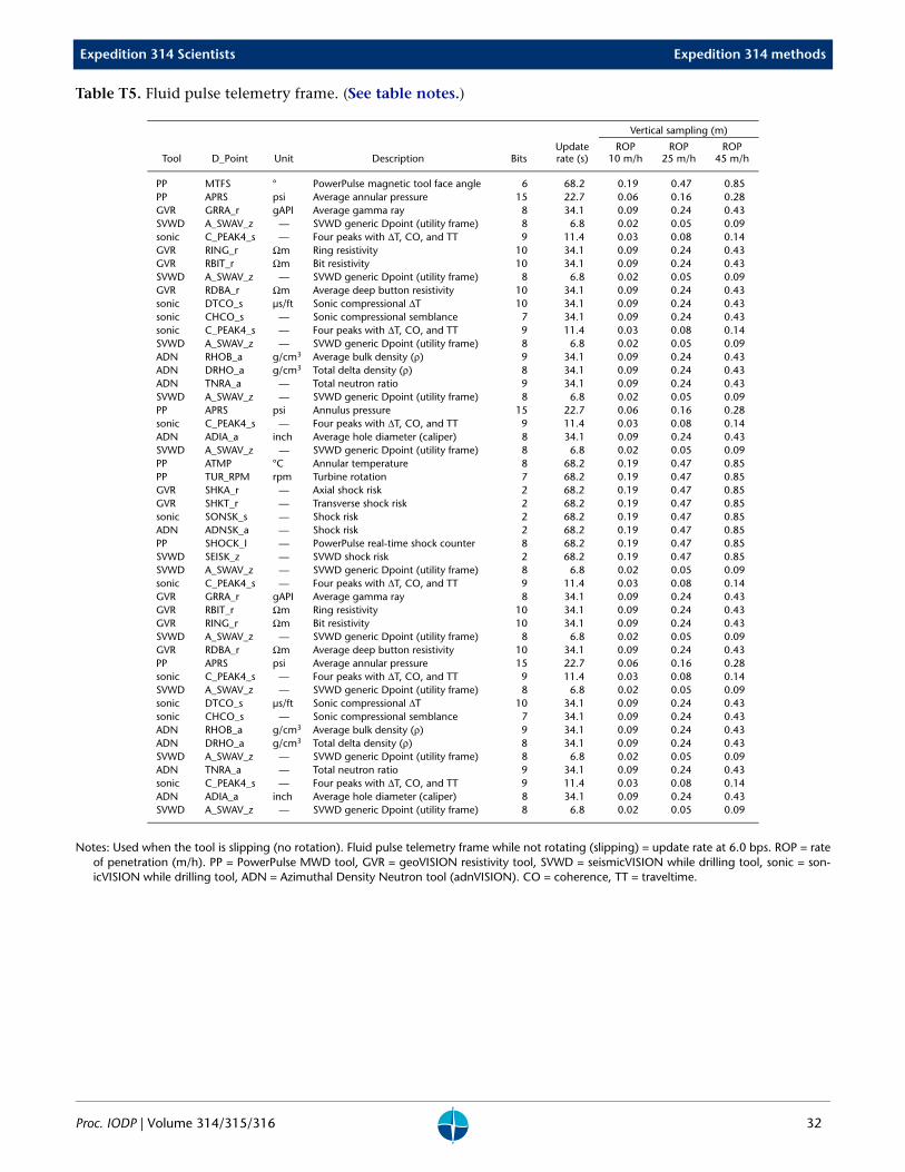
ateral shock sensors near the base of the MWD col-ar. A list of the main MWD parameters is given inable T1. Tables T4 and T5 list typical telemetryrames sent in real time, showing measurements re-orded using the MWD-APWD (PowerPulse) toolsnd their update rates. These data are transmitted tohe surface. The comparison of MWD drilling param-ters with rig instrumentation system data and shipeave information is used to improve drilling con-

rol and monitor any inflow or loss of circulationuring drilling.

uring LWD operations, the mud pulse system alsoransmitted a limited set of geophysical data fromhe adnVISION, geoVISION, sonicVISION, and seis-

icVISION LWD tools to the surface in real time.


These scientific measurements include gamma rayvalues, resistivity, bulk density, neutron porosity,compressional velocity (P-wave), and seismic wave-forms. Measurement parameters from each LWD col-lar were updated at rates corresponding to 15 cm to1.5 m depth intervals, depending on the initializedvalues and rate of penetration (ROP) of the tool (Ta-bles T4, T5). The combination of all these data con-firmed the operational status of each tool and pro-vided real-time logs for identifying lithologiccontacts and potential shallow-water flow or over-pressured zones. The real-time data also became theonly source of information in cases when the datarecorded in memory could not be retrieved (e.g., SiteC0001 adnVISION data and all data for Site C0003).

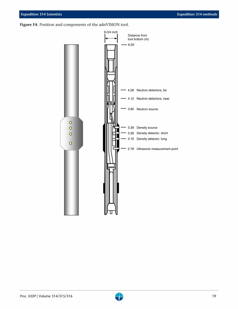
adnVISION toolThe adnVISION tool is similar in principle to theolder compensated density neutron tool (Anadrill-Schlumberger, 1993; Moore, Klaus, et al., 1998). Thedensity section of the tool uses a 1.7 Ci 137Cs gammaray source in conjunction with two gain-stabilizedscintillation detectors to provide a borehole-com-pensated density measurement (Table T6). The de-tectors are located 5 and 12 inches (12.7 and 30.48cm) below the source (Fig. F4). The number ofCompton scattering collisions (change in gamma rayenergy by interaction with the formation electrons)is related to the formation density (Schlumberger,1989).

Returns of low-energy gamma rays are converted to aphotoelectric factor (PEF) value, measured in barnsper electron. The PEF value depends on electron den-sity and therefore responds to bulk density and li-thology (Anadrill-Schlumberger, 1993). PEF value isalso particularly sensitive to low-density, high-poros-ity zones.

The density source and detectors are positioned be-hind windows in the blade of 8¼ inch (25.9 cm) in-tegral blade stabilizer. This geometry forces the sen-sors against the borehole wall, thereby reducing theeffects of borehole irregularities and drilling. Neu-tron logs are processed to eliminate the effects ofborehole diameter, tool size, temperature, drillingmud hydrogen index (dependent on mud weight,pressure, and temperature), mud and formation sa-linities, lithology, and other environmental factors(Schlumberger, 1994). The vertical resolution of thedensity and photoelectric effect measurements is ~6and 2 inches, respectively.

For measurement of tool standoff and estimatedborehole size, a 670 kHz ultrasonic caliper is avail-able on the tool. The ultrasonic sensor is alignedwith, and located just below, the density detectors.This sensor has an accuracy of ±0.1 inch and a verti-

3


P

css

NfbftTmm1f((otoim

Ttimfppdgprtometab1tcsS

Lfmefcmdsaet

al resolution of ~6 inches. In this position the sen-or can also be used as a quality control for the den-ity measurements.

eutron porosity measurements are obtained usingast neutrons emitted from a 10 Ci americium oxide-eryllium (AmBe) source. Hydrogen quantities in theormation largely control the rate at which the neu-rons slow down to epithermal and thermal energies.he energy of the detected neutrons has an epither-al component because much of the incoming ther-al neutron flux is absorbed as it passes through the

inch drill collar. Neutrons are detected in near- andar-spacing detector banks, located 12 and 24 inches30.48 and 60.96 cm), respectively, above the sourceFig. F4). The vertical resolution of the tool underptimum conditions is ~12 inches (34 cm). The neu-ron logs are affected to some extent by the lithologyf the matrix rock because the neutron porosity units calibrated for a water-saturated sandstone environ-

ent (Schlumberger, 1989).

he azimuthal measurement from the adnVISIONool is not reliable in wells with low deviation (<10°nclination). In such environments, an average or

aximum value should be used instead. Data outputrom the adnVISION tool include apparent neutronorosity (i.e., the tool does not distinguish betweenore water and lattice-bound water), formation bulkensity, and photoelectric factor. The density logsraphically presented here have been “rotationallyrocessed” to show the average density that the tooleads while it is rotating. In addition, the adnVISIONool outputs an inferred density caliper record basedn the standard deviation of density measurementsade at high sampling rates around the circumfer-

nce of the borehole. The measured standard devia-ion is compared with that of an in-gauge boreholend the difference is converted to the amount oforehole enlargement (Anadrill-Schlumberger,993). A standoff of <1 inch (2.54 cm) between theool and the borehole wall indicates good boreholeonditions, for which the density log values are con-idered to be accurate to ±0.015 g/cm3 (Anadrill-chlumberger, 1993).

ogging while drilling is a challenging environmentor formation density measurement. The measure-

ent is strongly affected by tool motion and influ-nced by the drilling fluid composition. The net ef-ect is formation density and PEF measurements thatan be inaccurate or misleading. The accuracy of theeasurements can be greatly improved by acquiring

ata in both depth and azimuthal dimensions, as-embling these data into a two-dimensional image,nd selecting the density measurements least influ-nced by borehole effects from this image. In LWDools, and in particular the adnVISION tool, azi-


muthal data are acquired most economically fromone set of sensors swept around the borehole by therotation of the drill string.

The image-derived density algorithm uses the com-pensated density image to compute a single compen-sated density. It identifies which sectors at eachdepth level provide the highest quality measure-ments and computes a density measurement basedon those sectors. It essentially automates what askilled log analyst does when interpreting a densityimage. The algorithm consists of the following threesteps:

1. Quality factor computation. For each depth leveland sector, the short- and long-spaced densitiesand volumetric PEF are used to compute a qualityfactor. The quality factor is based on qualitativeexpectations and an empirical choice of parame-ters. Larger quality factors represent more accu-rate density measurements.

2. Toolpath identification. As a function of depth,the centroid of the region of high-quality mea-surements defines a toolpath. The toolpath canbe thought of as the path of closest approach ofthe tool to the formation. This path is computedfrom the quality factor at each depth level by apartial Fourier decomposition.

3. Density calculation. The density is computed ateach depth level by averaging the bulk densityover four sectors centered on the toolpath. Frac-tional sectors are accounted for by linear inter-polation. These steps are described in detail inRadkte et al. (2003).

By construction, this algorithm yields the highestquality density and PEF measurements possible. Thistechnique has several other advantages: it is com-puted only from density sensor data, it is immune tothe statistical bias and limited applicability of maxi-mum density approaches, and the toolpath serves asa powerful quality control indicator.

geoVISION toolThe geoVISION resistivity tool is based on resistivity-at-the-bit (RAB) technology, which was designed toprovide real-time at-bit resistivity data. This explainswhy numerous geoVISION measurement acronymsinclude RAB in their name (see Table T3). The geo-VISION resistivity tool provides resistivity measure-ments and electrical images of the borehole wall, cal-ibrated in a homogeneous medium. In addition, thegeoVISION tool contains a scintillation counter thatprovides a total gamma ray measurement (Fig. F5).

The geoVISION tool is connected directly above thedrill bit and uses the lower portion of the tool andthe bit as a measuring electrode. This allows the tool

4


P

tclcvr(iiiilsTmesnsimvidmrr(

Tfwtghroom~ar

Tttb8tma

sTrwµ

o provide a bit resistivity measurement with a verti-al resolution just a few centimeters longer than theength of the bit. A 1½ inch (4 cm) electrode is lo-ated 102 cm from the bottom of the tool and pro-ides a focused lateral resistivity measurement (ringesistivity) with a vertical resolution of 2–3 inches5–7.5 cm). The characteristics of ring resistivity arendependent of where the geoVISION tool is placedn the BHA, and its depth of investigation is ~7nches (17.8 cm; diameter of investigation ≈ 22nches). In addition, button electrodes provide shal-ow-, medium-, and deep-focused resistivity mea-urements as well as azimuthally oriented images.hese images can then reveal information about for-ation structure and lithologic contacts. The button

lectrodes are ~1 inch (2.5 cm) in diameter and re-ide on a clamp-on sleeve. The buttons are longitudi-ally spaced along the geoVISION tool to rendertaggered depths of investigation of ~1, 3, and 5nches (2.5, 7.6, and 12.7 cm). The spacing provides

ultiple depths of investigation for quantifying in-asion profiles and fracture identification (drillingnduced versus natural). Vertical resolution andepth of investigation for each resistivity measure-ent are shown in Table T7. For environmental cor-

ection of the resistivity measurements, drilling fluidesistivity and temperature are also measuredSchlumberger, 1989).

he tool’s orientation system uses Earth’s magneticield as a reference to determine the tool positionith respect to the borehole as the drill string ro-

ates, thus allowing both azimuthal resistivity andamma ray measurements. The gamma ray sensoras a range of operability of 0–250 gAPI and an accu-acy of ±7% corresponding to a statistical resolutionf ±3 gAPI at 100 API and ROP of 30 m/h. Its depthf investigation is between 5 and 15 inches. The azi-uthal resistivity measurements are acquired with a

6° resolution, whereas gamma ray measurementsre acquired at 90° resolution as the geoVISION toolotates.

he geoVISION tool collar configuration is intendedo run in 8½ inch (22 cm) and 9 inch (25 cm) diame-er holes depending on the size of the measuringutton sleeve. During Expedition 314, we used an½ inch diameter bit and an 8¼ inch diameter but-on sleeve for the geoVISION tool. This resulted in a

inimum standoff between the resistivity buttonsnd the formation, giving higher quality images.

onicVISION toolhe sonicVISION sonic-while-drilling tool deliverseal-time interval transit time data for compressionalaves. The available measurement range is ~40–230s/ft (1.3–7.6 km/s), depending on mud type, but in-


tensive processing was sometimes required to obtainreliable sonic velocity measurements in the relativelyslow formations drilled during Expedition 314. Inreal-time LWD operations, the sonic processing pa-rameters are conventionally set at the surface beforethe tool is run in the hole. The real-time projectionlog and labeling with quality control log affect thereal-time slowness and quality of the data. This re-sults in the possible mislabeling of arrivals (espe-cially for slow formations) and limited confidencelevels, as only the end result of downhole processingis seen uphole in the real-time log. In general, duringExpedition 314 the real-time sonic traveltimes werespurious and unreliable; however, full waveformdata are recorded in memory. Advanced onboardpostprocessing extended the range of measurementto near the mud velocity, a key feature for achievingthe scientific objectives of this cruise, including log-seismic ties. Additional quality control is performedusing automatic stationary measurements made dur-ing a pipe connection. In this less noisy environ-ment, the tool is able to take a station measurementthat is sent uphole, when pumping resumes, for fur-ther quality control of the real-time log (Fig. F6).

The wideband frequency measurement and high-power transmitter have been improved from theolder tool. Wideband frequency measurements re-duce aliasing and eccentralization effects, improveformation signal strength, and allow measurementof shear and Stoneley waves. The transmitter outputslarge amounts of wideband power to effectively cou-ple more energy into various formation types, ulti-mately improving the signal-to-noise ratio and,therefore, measurement quality and hole size range.Extended battery life, large memory capacity, andfast dump speed significantly enhance thesonicVISION tool’s reliability and functionality.Standard memory life is 140 h at 10 s acquisition,and this is easily doubled. In addition, standardized“planning” software allows the engineer to easily op-timize the tool configuration for the well beingdrilled.

In shallow unconsolidated formations where thecompressional velocity approaches or is below thefluid (mud) velocity, it is difficult to directly measurethe formation slowness with the refracted wave be-cause the energy of the refracted wave is too weak.When the compressional slowness is larger than themud slowness, a significantly low frequency (severalkilohertz) source is needed to measure the formationslowness (Wu et al., 1995). However, if the compres-sional slowness is close to the mud slowness but stillsmaller than the mud slowness, the formation slow-ness can be extracted with processing a leaky com-pressional (“leaky-P”) mode excited by a wideband

5


P

s(cTfacthmtttfsict

SwHdareplatwt

TabmsaT1pvpgmwSs

sTdiccd

ource. Tichelaar and Luik (1995) and Valero et al.1999) discussed the compressional slowness pro-essing in such conditions for wireline sonic data.hey processed a leaky-P mode by applying a lowerrequency band-pass filter to attenuate fluid modesnd enhance formation arrivals. The leaky-P modeonsists of multiple reflected and constructively in-erfering compressional waves traveling in the bore-ole fluid (Paillet and Cheng, 1991). The leaky-Pode is dispersive, such that at lower frequencies

he slowness asymptotically approaches the forma-ion compressional slowness and at higher frequencyo the mud slowness. Because of this dispersive ef-ect, the slowness estimated by the nondispersiveemblance processing (Kimball and Marzetta, 1984)s greater than the true P-wave slowness. Therefore,orrection for dispersion is needed in order to obtainhe true formation compressional slowness.

tandard LWD-sonic measurements are operatedith a frequency band of ~11 kHz (Aron et al., 1997).owever, in the case of a very slow formation, it isifficult to obtain the compressional slowness using standard source because the energy of the fluid ar-ivals dominates those of the leaky-P mode. It is nec-ssary to expand the source spectrum of the mono-ole transmitter to lower frequencies to excite the

eaky-P mode. Therefore, wide frequency band datacquisition is required to excite a leaky-P mode. Bothhe semblance processing and the dispersive analysisith Prony method (Ekstrom, 1995) clearly showed

he existence of dispersive leaky modes.

he modeling of leaky-P dispersion has to take intoccount a realistic tool structure for a wide range oforehole and formation parameters. Based on theseodeling results, a correction table for the disper-

ion biases is established and dispersion correctionpplied to obtain formation compressional slowness.his procedure was applied to the ODP logs from Leg96 Hole 1173B and Leg 130 Hole 808I and com-ared with the core slownesses measured on the pre-ious leg (Mikada et al., 2002). The result of the dis-ersion-corrected LWD sonic processing showedood agreements with these core velocity measure-ents (Goldberg et al., 2005). A similar procedureas applied by the Schlumberger Data Consulting

ervice (DCS) specialist for onboard processing ofonic data.

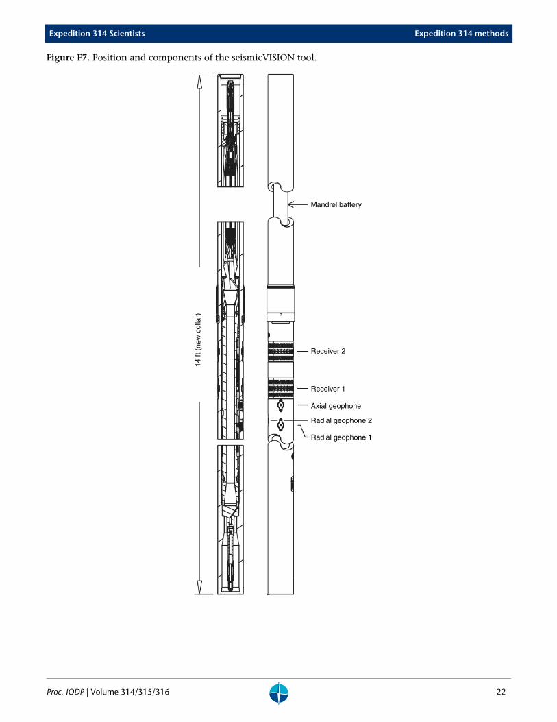
eismicVISION toolhe seismicVISION LWD system delivers time- andepth-velocity information to provide interval veloc-

ty. The seismicVISION tool, which contains a pro-essor and memory, receives seismic energy from aonventional air gun suspended from a crane on therillship. After acquisition, the seismic signals are


stored and processed downhole, and check shot dataand quality indicators are transmitted uphole in realtime by connection with the MWD pulse system.Waveforms are recorded in the tool memory for fur-ther processing after a bit trip. Refer to “Log-seismiccorrelation” for more information (Fig. F7).

Onboard data flow and quality check

For each operation, two types of data are collected:(1) real-time data that include all MWD-APWD dataand selected LWD data and (2) LWD data that havebeen recorded downhole and stored in the tool’smemory. Data are originally recorded downhole at apreset frequency. The depth version is obtained aftermerging the time (downhole) with the time-depthrelationship recorded on the surface by the IDEALsystem. For the MWD-APWD, adnVISION, and geo-VISION tools, both time and depth versions of thedata exist. The raw sonicVISION data were only dis-tributed versus depth and were processed onboardby the DCS specialist. In the same way, the seis-micVISION data (check shots) were only availableversus depth and distributed to the Shipboard Sci-ence Party for immediate processing and analysis.The time version of the data was made available inlog ASCII standard (LAS) format. The depth versionof the data was made available in digital logging in-terchange standard (DLIS) format for the MWD-APWD, adnVISION, geoVISION, and sonicVISIONtools and in Society of Exploration Geophysicistsstandard (data format “Y”) for the seismicVISIONtool.

After determining the position of the mudline byidentifying a break in the gamma ray log (and resis-tivity logs, when available), the data were depthshifted to the seafloor (LWD depth below seafloor[LSF]). The depth-shifted version of the MWD-APWD, adnVISION, geoVISION, and processed datawere distributed in the native format (DLIS), and themain scalar logs were extracted and converted intoLAS files. All files (time based, depth based, original,and depth shifted) and associated documentation(quality check and operation reports) were distrib-uted to the Shipboard Science Party through the on-board intranet data servers. Analyses, integration re-sults, and reports produced by the ShipboardScientific Party were then archived on the server forfurther distribution. Normal data flow is illustratedin Figure F8.

The Logging Staff Scientist performed initial conver-sion and output of the raw data received from theWellsite Geologist, who received the data from theSchlumberger LWD engineer. Logging Staff Scientist

6


P

dLiiadsvsddpias(dsiybdhbsctpdmmaatta

Qbo

GbDad

uties include documentation of the MWD-APWD-WD operations, data quality assessment (highlight-ng any abnormalities), depth shifting (i.e., convert-ng depth below rig floor to depth below seafloor),nd systematic distribution and documentation ofata. Operations and quality assessment are de-cribed in two main plots (data versus time and dataersus depth) related by a third time-depth relation-hip plot (Fig. F9). In the first plot (Plot 1), time-epth relationship (Panel 1.1), surface drilling andownhole parameters (Panel 1.2), and selected geo-hysical logs (Panel 1.3) are plotted versus time to

dentify the sequence of drilling events and furtherssess their possible impact on data quality. In theecond plot (Plot 2), the time-time relationshipPanel 2.1) and operational surface and downholeata (Panel 2.2) are reported versus depth for large-cale assessment of drilling conditions on data qual-ty. These first panels are completed by detailed anal-sis of the ultrasonic caliper, density, correction onulk density, and comparison of the shallow andeep button resistivity scalar logs to further assessole condition (cave, washout, or bridge) and possi-le impact on density/porosity data, as well as inva-ion (Panel 2.3). Elapsed time of the main geophysi-al measurements after bit is also indicated in thishird panel. In a fourth panel (Panel 2.4), changes inarameters of the sonic processing and a quality in-icator of the resulting processed sonic log are docu-ented. Finally, results of detailed quality assess-ent of borehole images (mostly shallow, medium,

nd deep button resistivity and gamma ray images)re documented in the last panel (Panel 2.5). Thehird time-depth relationship plot (Plot 3), made athe same scale as the two main time and depth plots,llows easy navigation between those two plots.

uality of MWD-APWD-LWD data is mostly assessedy cross-correlating available logs. Available logs aref two types, as follows:

1. Drilling control logs including surface drillingsurface parameters (e.g., ROP, surface weight onbit [SWOB], hook load [HKLD], standpipe pres-sure [SPPA]), and downhole drilling parameters(e.g., collar [bit] rotation [CRPM], hole deviation[HDEVI], radial shock rate [SKR_R], tangentialshock rate [SKR_T], shock peak [SHKPK], andstick-slip indicator [SLIP]) and

2. Geophysical control logs such as calipers (ADIA,ECAL_RAB), gamma ray (GR), annular pressure(APWD), and temperature (ATMP_MWD).

eophysical logging data may be degraded whereorehole diameter greatly increases or is washed out.eep investigation measurements such as resistivitynd sonic velocity are least sensitive to borehole con-itions. Nuclear measurements (density and neutron


porosity) are more sensitive because of their shallowdepth of investigation and the effect of drilling fluidvolume on neutron and gamma ray attenuation.Corrections were applied to the original data to re-duce these effects. The effects of very large washouts,however, cannot be corrected.

Azimuthal measurements and associated images areof low quality when the tool is not rotating (slip) orwhen its rotation exceeds 250 rpm. In zones of highstick-slip, even if tool rotation (CRPM) is set to a typ-ical value of 100 rpm, CRPM can greatly vary locally(and exceed 250 rpm), resulting in images of lowerquality. As all measurements even by the same toolare not sampled at the same time (sampling rate ofadnVISION and geoVISION = 5 s), improper heavecompensation and irregular movement of the BHA(vibration shocks or bending) can result in localdepth shift between measurements by several tens ofcentimeters.

Log characterizationand lithologic interpretation

LWD measurements provide in situ petrophysical in-formation on rocks and pore fluids while the hole isbeing drilled. These measurements are sensitive tochanges in composition (changing curve magni-tudes), textures, and structures (log shape, peak am-plitude, and frequency, as well as information fromimage logs). Changes in the log response (valuesand/or frequency of the signal) are commonly asso-ciated with geological unit boundaries.

This section addresses the characterization of theLWD measurements and imaging tool response, fo-cusing on zoning the well logs into logging units.Once representative petrophysical properties for thelogging units were defined, they were incorporatedin the log-based lithologic units. This process can beachieved by qualitative and quantitative methods.

Log characterization and identificationof logging units

Qualitative analysis The geometry of logging unit boundaries and bed-ding information was defined on the basis of bore-hole images and characterized from scalar LWD logs.Rock textures and structures were analyzed on bore-hole images, and vertical trends were analyzed on allthe available logs. Composition and textural infor-mation was derived mainly from nuclear (spectralgamma, density, and PEF) and sonic logs. Data qual-ity assessment was made by shipboard scientiststhrough the examination of the potential effect ofborehole diameter and conditions and drilling pa-

7


P

rr

Tiopdb

Ic

•

•

•

QAtptv

LDbotgc

CauttmwhstA1Sl

Ttpu

ameters on the logs prior to interpretation of the logesponse.

he first qualitative approach to unit definition wasdentification of the boundaries separating sectionsf different log responses and concomitant rockroperties. For this type of analysis, natural- and in-uced-radioactivity logs, sonic logs, resistivity, andorehole images were the main input.

ntegrated interpretation of all the available logs fo-used on the following items:

Definition and characterization of logging units,subunits, and unit boundaries;

Identification of compositional features withineach unit; and

Interpretation in terms of geological features (unitboundaries, transitions, sequences, and likely lith-ologic composition).

uantitative analysiss a consistency check of the qualitative interpreta-

ion and for quantitative log characterization, we ap-lied statistical grouping. This involved investigatinghe percentile ranges and distribution of absolutealues within the visually defined logging units.

og-based geological/lithologic interpretation uring Expedition 314, lithologies were interpretedased only on LWD logs without cores, unlike previ-us ODP/IODP expeditions. After log characteriza-ion and classification, logs were lithologically andeologically interpreted using a combination of logharacteristics and borehole images for each site.

ompositionally influenced logs such as gamma raynd PEF logs were used to determine lithology fromnit scale to bed scale. In particular, the identifica-ion of sand-rich intervals, clay-rich intervals, or al-ernating beds of sand and clay was a primary ele-

ent of the interpretation. Sonic and all other logsere also used for lithology characterization. Bore-ole images provided useful information on meso-copic features such as bedding, sedimentary struc-ures, bed boundaries, unconformities, and faults.dditionally, lithologic information from ODP Legs31, 190, and 196, all in the Nankai Trough offhikoku Island, was an important aid in interpretingithology.

hese interpretations will be confirmed by correla-ion with core data from subsequent NanTroSEIZEroject expeditions. A possible correlation to seismicnits was also proposed for each site.


Physical propertiesThe principal objectives for physical property analy-sis of the logging data concern the mechanical stateand physical properties of sediments in the accre-tionary prism, Shikoku Basin, and the trench fill, aswell as in the tectonic features. It also concerns theassessment of hydrogeologic conditions inferred onthe basis of physical property data.

The standard downhole logs provide information ona wide range of in situ physical properties. This in-cludes P-wave velocity, electrical resistivity, gammaray intensity, bulk density, and porosity.

In each site chapter, the physical properties sectionpresents the logs mentioned above as a function ofdepth and describes their features and their variationin conjunction with lithology, structural geology,and log-seismic integration. The bulk density log isplotted mainly using adnVISION image-derived bulkdensity (Schlumberger mnemonic IDRO) data. WhenIDRO data were not available, bulk density (RHOB)was used instead. The porosity log is plotted usingthermal neutron porosity (TNPH) and is derivedfrom bulk density for comparison. Ring; bit; andshallow, medium, and deep button resistivity logs indifferent measurement configurations are comparedagainst each other to examine measurement condi-tions and applied corrections. P-wave velocity is cal-culated and plotted as the inverse of compressionalwave slowness from the Schlumberger sonicVISIONtool (DTCO).

Estimation of porosity from the density logA density-derived porosity log is calculated from thebulk density log using the assumption of a constantgrain density (ρg) of 2.65 g/cm3 and a constant waterdensity (ρw) of 1.024 g/cm3 (Blum, 1997). In the ab-sence of grain density measured on cores from thesame site, we based the value of the constant densityon previous measurements in the Nankai accretion-ary prism area off Muroto during Leg 190 (Moore,Taira, Klaus, et al., 2001). The equation used to de-rive the porosity (ϕ) from the bulk density log (ρb) is

.

Estimation of porosityfrom the resistivity log

Archie’s law (Archie, 1947) is usually used to derive aporosity log from the resistivity log as

ϕρb ρg–ρw ρg–------------------=

8


P

wmdtmtcttrA

T

wfsrt

Tcscat

Ttlcmb

SVm((past

Tiv~

,

here F is the formation factor, a is a constant, and is the so-called cementation factor. The variable mepends on rock type and is more closely related toexture than to cementation. Several values of a and can be found in the literature. The actual values of

he a and m parameters will be explained in each sitehapter. One limitation of this simple approach ishat it does not take lithology or pore fluid varia-ions into account. It should also be noted that theesulting estimate is very sensitive to the choice ofrchie’s law constants.

he formation factor is calculated as

,

here R is the LWD-measured resistivity and Rf is theluid resistivity. We assumed that the pore fluid isimilar to seawater. The formula used to calculate theesistivity of seawater (Rf) as a function of tempera-ure T (°C) is as follows (Shipley et al., 1995):

.

he temperature profile was calculated at each siteonsidering a conductive heat transfer, the measuredurface heat flux, and an estimation of the thermalonductivity based on previous coring in the Nankaiccretionary prism. The value used for this calcula-ion is defined in each site chapter.

he bit resistivity measurement was used for this es-imation because this is the measurement with theargest depth of investigation (12 inches) and be-ause the position at the bit of the tool string mini-izes the effect of formation modification induced

y drilling.

Structural geologyand geomechanics

tructural analysis was performed primarily on geo-ISION resistivity images using GMI Imager (Geo-echanics International Inc.), GeoLog/Geomage

Paradigm Geotechnology B.V.), and GeoFrameSchlumberger) software. These software packagesresent resistivity image data of the borehole wall as planar “unwrapped” 360° image with depth. Theoftware also allows visualization of the data in ahree-dimensional (3-D) borehole view.

he geoVISION downhole tool provides resistivitymages of shallow, medium, and deep depths of in-estigation, imaging the formation at ~34, ~43, and55 cm diameters of investigation, respectively. Re-

F aϕm-------=

F RRf

----=

Rf1

2.8 0.1T+---------------------------=


sistivity image data were imported into the softwarepackages and displayed as both statically and dy-namically normalized images. Static normalizationdisplays the image with a color range covering all re-sistivity values for the entire logged interval. Staticnormalization is preferred for comparing relativechanges in resistivity throughout the borehole and istherefore ideal for correlating lithologic or facieschanges and comparing the resistivity of particularfault zones. Dynamic normalization scales the colorrange for resistivity values over a specified interval.Dynamic normalization is commonly used for de-tailed identification of fractures and sedimentarystructures and often allows more subtle changes inthe image to be identified. Further filtering of thedata was also possible with the software. Image datawere compared with borehole caliper data to investi-gate the changing average diameter of the borehole.

Methods of interpreting structure and bedding differconsiderably between cores, wireline logs, and LWDdata sets. Horizontal and vertical resolution of resis-tivity images is considerably lower than comparabledata from cores and wireline image logs (e.g., Full-bore Formation MicroImager [FMI]). Vertical resolu-tion for LWD resistivity images is ~5–7.5 cm if ROP ismaintained at ~20–30 m/h. Horizontal resolutionacross the image is a function of several factors.Some of these factors cannot be precisely con-strained; therefore, this resolution has some uncer-tainty. These factors include the diameter of investi-gation (i.e., shallow, medium, or deep), which is alsoinfluenced by borehole elongation; the differencebetween formation resistivity and that of the bore-hole fluid; and the number of measurements madearound the hole (56 for the geoVISION tool). The ra-tio between Rt (true resistivity of formation) and Rxo

(resistivity of zone invaded by drilling fluid) also in-fluences the diameter of investigation, but we as-sumed the ratio to be 1.0, owing to minimal inva-sion because resistivity was measured soon afterdrilling. For the geoVISION tool and the likely rangeof formation resistivities encountered during this ex-pedition, the approximate horizontal resolutionsrange from ~2 to 3 cm. The ability to image a feature(feature detection) is also a function of the resistivitycontrast and resolution. It may therefore be possibleto resolve features smaller than the expected verticalor horizontal resolution if they contrast stronglywith the background resistivity. The vertical resolu-tion also controls whether the thickness of a layercan be determined. These resolutions should becompared with cores (millimeters) and FMI wirelineresistivity images (~0.5 cm); therefore, smaller fea-tures are not resolvable within the LWD images. Forexample, individual microfaults (“small faults” <1

9


P

mwbsp

InbadwmtrywGcgfp

WiidtotrfbDpibclsdcb

BisrtpsBp

m width) and shear bands (1–2 mm to 1 cm inidth) identified in cores (e.g., Site 808) should note resolvable in LWD resistivity image data. Thishould be considered when directly comparing re-orts from previous and future data sets.

n the unwrapped geoVISION resistivity images, si-usoidal lines are planar surfaces inclined to theorehole axis. Curved lines differing from sinusoidsre nonplanar surfaces. To pick planar features (bed-ing planes, beds, fractures, faults, etc.), sinusoidsere interactively fitted to determine dip and azi-uth. Features were further classified according to

ype of fracture, width/aperture, shape, and relativeesistivity (conductive versus resistive). Further anal-sis (fracture frequency, azimuth distribution, etc.)as performed in GMI Imager, GeoLog/Geomage,eoFrame, and other software packages. We also

ompared resistivity images directly with other log-ing data for interpretation of bedding planes andor correlation of deformation style, lithology, andhysical properties.

e identified fractures within geoVISION resistivitymages by their contrasting resistivity or conductiv-ty, from contrasting dip relative to surrounding bed-ing trends, or by truncation of other features. Resis-ivity of fractures is defined relative to the full rangef resistivity values within the hole and is nonquan-itative. If relative resistivity is unclear, the fractureesistivity is undefined. In some cases, conductiveractures may be easier to identify relative to theackground resistivity, biasing the results slightly.ifferentiation between fractures and beddinglanes is complex and less accurate where bedding is

nclined. Care was taken to avoid misinterpretingorehole artifacts as natural geological features. Weompared initial structural interpretations from theogging data with seismic reflection data. Compari-ons with cores will be possible following later expe-itions. Our interpretations are based on the aboveriteria, but we acknowledge that some fractures andedding planes may have been misinterpreted.

Borehole wall failure analysisreakouts and/or tensile fractures, two types of drill-

ng-induced borehole wall failure, form when thetate of local stress field at the borehole wall exceedsock/sediment strength. Breakouts form parallel tohe minimum principal horizontal stress (Shmin) anderpendicular to the maximum horizontal principaltress (SHmax), resulting in elongation of the borehole.reakouts are recorded in resistivity images as twoarallel conductive vertical features 180° apart. Drill-


ing-induced tensile fractures may form in conjunc-tion with breakouts or independently. The tensilefractures form perpendicular to Shmin, 90° from theazimuth of the breakouts.

We recorded the orientation, downhole extent, andwidth of breakouts with the image analysis softwareconsidering all three borehole images (shallow, me-dium, and deep). Caliper data allow visualization ofthe changing average borehole diameter with depth,but azimuthal caliper data were not referenced to geo-graphic coordinates and so cannot be used to assessborehole elongation. We compared breakout distribu-tion and width with lithology (from image resistivityand defined lithologic units derived from all loggingdata) and drilling parameters. Further breakout analy-sis was conducted with GMI and other software.

Constraining stress from drilling-induced tensile fractures

Drilling-induced tensile fractures occur when thehoop stress at the borehole wall exceeds rock tensilestrength. Where the tensile strength of sediments isnegligible, the occurrence of drilling-induced tensilefractures is an indicator of tensile hoop stress at theborehole wall. We attempted to estimate in situstress magnitudes by constraining possible stressranges that allow failure in the borehole, specificallythe formation of drilling-induced tensile fractures.Most of the following discussion is drawn fromZoback et al. (2003).

Because the stress in sediment is limited by thestrength of frictional sliding on faults, it is possibleto constrain the range of possible stress states at anydepth and pore pressure. If the ratio between the twoextreme effective principal stresses goes beyond cer-tain values defined by the coefficient of friction, slid-ing occurs along critically oriented faults (Byerlee,1978), which in turn releases the excess stresses.More explicitly, the limiting condition for failure canbe expressed by Coulomb friction law:

,

where µ2 is the coefficient of friction, Pp is pore pres-sure, and S1 and S3 are the maximum and minimumin situ principal stresses, respectively. This equationcan be plotted as three lines (1, 2, and 3 in Fig. F10)representing the conditions of failure and definingthe “stress polygon” in the SHmax versus Shmin or hori-zontal stress domain. This stress polygon encom-passes the possible states of stress at a given depth.

S1 PP–S3 PP–---------------- μ2 1+ 1+( )

2=

10


P

AmTvfsga

Isruifapws

Efcrfeep(scsgrwtw

Ddm2tf

Tivfup

bove and to the left of these three lines the sedi-ent/rock would be at failure in its natural state.

he interiors of the stress polygons define allowablealues for horizontal principal stresses for conditionsavoring but not at the threshold of normal, strike-lip, and thrust faulting. The size of the stress poly-on depends on the coefficient of friction, depth,nd pore pressure.

ODP holes provide information on the verticaltress from the overburden, borehole pressure by di-ect downhole measurements with MWD tools, fail-re through the presence of breakouts and drilling-

nduced tensile fractures, and potentially, style of de-ormation from offset features. These observationsre used with the theoretical framework above torovide estimates of the stresses in the borehole andhether the stress ratios favor normal, thrust, or

trike-slip faulting.

stimation of stress magnitude is possible when in-ormation on rock strength is available. Since noore was recovered from this LWD expedition, indi-ect estimations of rock strength parameters (uncon-ined compressive strength and internal friction co-fficient) were made using a set of empiricalquations that relate rock strength to other physicalroperties measured from geophysical loggingChang et al., 2006). The two strength parameters areufficient to construct any well-known rock strengthriteria (Colmenares and Zoback, 2002). We used atrength criterion that is suitable for describing theeneral strength characteristics of the sedimentaryock. Ranges of possible in situ stress magnitudesere constrained by comparing rock strength with

he state of the local stress field at the borehole wallhere we observed borehole breakouts.

Log-seismic correlationuring Expedition 314 we used several of the LWData sets to establish accurate ties to the 2006 Ku-ano 3-D seismic reflection data set (Moore et al.,

007). Data from seismicVISION and sonicVISIONools helped to establish a traveltime to depth trans-orm at the boreholes.

seismicVISION toolhe seismicVISION tool produces data which can be

nterpreted as a check shot survey, a low-resolutionelocity depth function, and a vertical seismic pro-ile. The seismicVISION tool records seismogramssing a hydrophone and a three-component geo-hone in the tool and a surface source and hydro-


phone (www.slb.com/content/services/drilling/imaging/seismicvision.asp). The source was three250 in3 air guns (Fig. F11) that were suspended fromcrane 1 ~55 m horizontally from the rotary table(Fig. F12) and fired 6 m below sea level at 1700–2000 psi. Time correlations of the shots are ensuredusing high-precision clocks at both the surface hy-drophone and downhole hydrophone. The surfacehydrophone was suspended 3 m below the air guns(total 9 m below mean sea level) and the zero timesof the waveforms were corrected to mean sea level.

Data cannot be usefully obtained when the pipe isrotating or moving vertically or when the drillingfluid pumps are running. Therefore, seismicVISIONdata are typically acquired at each addition or re-moval of a stand of drill pipe (~38 m long) to or fromthe drill string. The Chikyu uses four joints (9.5 mlong drill pipe) as one stand. The drill string is sta-tionary and the pumps are off during these times.This means that while drilling the hole, data were ac-quired every 38 m. After drilling was complete andwhile the pipe was being recovered, data were alsoacquired every 38 m but at points shifted by twojoints (19 m) relative to the acquisition during drill-ing. Thus, combining the data acquired during drill-ing and the data acquired during pipe recoveryyielded data nominally acquired at 19 m intervals inthe borehole (Fig. F13).

At each data acquisition level, a number of shotswere fired by the surface source. When rig circula-tion/rotation stopped, the seismicVISION acquisi-tion system was activated. The source was fired at 15s intervals. The time for the insertion or removal of apipe stand was at least 3 min. Thus, the standardprocedure was to fire 10–15 shots. The tool recordsthe pressure (hydrophone) and acceleration (three-component geophones) seismograms obtained foreach shot and calculates and records a vertical stackof the shots. In practice, because our holes were nearvertical and the tool was centered and unclamped,the geophone data yielded little useful information.The tool also automatically picks and records the P-wave arrival time in the stacked seismogram. Thestacked seismogram and the picked P-wave arrivaltimes from the instrument are transmitted to theship by the MWD system and thus could be usedsoon after acquisition at each level or as the primarydata in case the tool fails to record data or is lost.

A check shot survey consists of the one-way first ar-rival traveltimes of a seismic pulse from the surfaceto a downhole hydrophone placed at a series ofknown depths in the hole. This corresponds to thepicked P-wave arrival at each depth from the seis-

11

http://www.slb.com/content/services/drilling/imaging/seismicvision.asp

http://www.slb.com/content/services/drilling/imaging/seismicvision.asp


P

mfddt

Wsisw

AtddmoLffso

Abhtigtzsdpmfmd

WtptdisM

SWbnt

icVISION tool. This was the most reliable data setor matching seismic reflectors acquired in the timeomain with logging and core data acquired in theepth domain. The check shot data are a key inputo the process of making a synthetic seismogram.

e processed the seismicVISION data using ProMAXoftware (Landmark-Halliburton). After manual edit-ng of bad or noisy traces and frequency filtering, thehots from each level were stacked and first breaksere picked.

velocity depth function was obtained by takinghe differences between adjacent vertical traveltimeata (the check shot data) and dividing by the depthifference. Velocity depth curves obtained in thisanner are typically quite noisy. A smooth version

f this curve was obtained using the methodology ofizarralde and Swift (1999). This curve may be use-ully compared with the velocity versus depth datarom the sonicVISION tool and with the velocity ver-us depth at the hole location used in the processingf the 3-D seismic volume.

vertical seismic profile can be obtained by assem-ling a gather of the stacked seismograms from aole sorted by receiver depth. This gather was fil-

ered to remove noise and the upgoing and downgo-ng waves were separated using FK filtering. The up-oing arrivals were then moved out (flattened inime) and stacked to produce an equivalent of theero-offset reflection seismogram, called a corridortack, at the hole location. When the seismicVISIONata are of very high quality, this stack should com-are favorably with the hole location trace in the 3-Dultichannel seismic (MCS) reflection volume. Dif-

erences in arrival times between these seismogramsay indicate problems with the velocity field used to

epth migrate/convert the MCS data.

Depth conversion of seismic reflection datae used the time-depth transforms obtained from

he seismicVISION data to convert the originalrestack time-migrated 3-D seismic reflection data tohe depth domain for correlation with the LWData. For each site we made depth conversions of an

nline seismic section that passes through the drillite (100 traces on each side of the site using Pro-AX seismic processing software).

ynthetic seismogramse constructed synthetic seismograms using the

est available density curve and the detailed slow-ess (inverse of velocity) log from the sonicVISION

ool. Where the sonicVISION tool was not working


properly, because of slow formations or other com-plications, we generated a velocity curve from thedensity log using the Gardner equation (Gardner etal., 1974).

Conversion from time to depth was required duringsynthetic seismogram construction to allow correla-tion of the depth-based LWD logs to the traveltime-based seismic data. This conversion was done usingthe check shot data generated by the seismicVISIONtool to generate a traveltime to depth relationship.

The sonicVISION tool provides good information forinterval velocity changes at short wavelengths. TheseismicVISION tool, after processing and filtering,provides a reliable smooth interval velocity curve atlong wavelengths. Following general industrial prac-tices, we took the smoothed interval velocity curvefrom the check shot as correct and calibrated thesonic log so that these two curves matched in theirtime to depth relationships. This calibration isachieved by creating a drift curve that shifts thesonic log within defined intervals (based on inflec-tion points in the drift curve) while preserving theshorter wavelength relative velocity changes pro-vided by the sonic data.

To create a synthetic seismogram, a source waveletwas convolved with a reflectivity series usingGeoFrame software (Schlumberger). The reflectivityis expressed in the following form:

R = (ν2ρ2 – ν1ρ1)/(ν1ρ1 + ν2ρ2),

where ν1, ν2 and ρ1, ρ2 are the acoustic velocity anddensity in the upper layer and lower layer, respec-tively. For Expedition 314, we estimated the sourcewavelet from the best waveform and amplitudematch provided by wavelets extracted within 20traces of each site in the orientation (inline or cross-line) providing the flattest seafloor. We used a deter-ministic extraction method based either on the en-ergy or power spectrum and in each case let the soft-ware define the best wavelet length and lag. Toobtain a wavelet we defined a start and end timewithin the trace, always starting shallower than theseafloor and ending deeper than the wavelet length.The software computes a zero lag autocorrelation ofthe reflection coefficients from each trace within theregion defined and then computes a signal-to-noiseratio for each trace. An optimal inline/cross-line pairis returned along with an optimal time lag that re-sults in the highest signal-to-noise ratio and thatpasses a 90% confidence level based on normalizedmean square error (NMSE). We determined the opti-mal wavelet length by computing the best length at

12


P

embclfgcbwltseswtt

UbfvaDmfq

A

A

A

B

B

C

C

E

ach site using the portion of energy predicted (PEP)ethod. In this method, a wavelet is generated

ased on the deterministic method (power spectrumomparison or energy comparison) for each wave-ength to be tested and then convolved with the re-lection coefficient to generate a synthetic seismo-ram. The resulting synthetic seismogram is thenompared to the input trace based on its PEP and theest match wavelet length is returned. The optimumavelet lengths in all cases proved to be 256 ms, the

ags varied some but were usually close to zero, andhe extracted wavelets were all zero phase. For eachite, we varied the start and end time for the waveletxtraction window and tried both energy and powerpectrum comparisons until we attained a sourceavelet that had high signal-to-noise ratio, passed

he NMSE test, and visually provided the best fit tohe frequency spectrum of the input data.

sing the check shot curve, calibrated sonic log, andest available density log we were able to create a re-lection coefficient series. This series was then con-olved with the extracted source wavelet to generate synthetic seismogram at a 4 ms sampling interval.isplaying the synthetic seismogram beside the seis-ic data from the area of the borehole provides in-

ormation about specific boundaries of interest and auality check on velocity and density logs.

Referencesnadrill-Schlumberger, 1993. Logging While Drilling: Hous-

ton (Schlumberger), SMP-9160.rchie, G.E., 1947. Electrical resistivity—an aid in core

analysis interpretation. AAPG Bull., 31:350–366.ron, J., Chang, S.K., Codazzi, D., Dworak, R., Hsu, K., Lau,

T., Minerbo, G., and Yogeswaren, E., 1997. Real-time sonic logging while drilling in hard and soft rocks. Trans. SPWLA Annu. Logging Symp., 38:1HH–14HH.

lum, P., 1997. Physical properties handbook: a guide to the shipboard measurement of physical properties of deep-sea cores. ODP Tech. Note, 26. doi:10.2973/odp.tn.26.1997

yerlee, J., 1978. Friction of rocks. Pure Appl. Geophys., 116(4–5):615–626. doi:10.1007/BF00876528

hang, C., Zoback, M.D., and Khaksar, A., 2006. Empirical relations between rock strength and physical properties in sedimentary rocks. J. Pet. Sci. Eng., 51(3–4):223–237. doi:10.1016/j.petrol.2006.01.003

olmenares, L.B., and Zoback, M.D., 2002. A statistical evaluation of intact rock failure criteria constrained by polyaxial test data for five different rocks. Int. J. Rock Mech. Min. Sci., 39(6):695–729. doi:10.1016/S1365-1609(02)00048-5

kstrom, M.P., 1995. Dispersion estimation from borehole acoustic arrays using a modified matrix pencil algo-rithm. Signals, Syst. Comput., 1:449–453. doi:10.1109/ACSSC.1995.540589


Flemings, P.B., Behrmann, J.H., John, C.M., and the Expe-dition 308 Scientists, 2006. Proc. IODP, 308: College Sta-tion TX (Integrated Ocean Drilling Program Management International, Inc.). doi:10.2204/iodp.proc.308.2006

Gardner, G.H.F., Gardner, L.W., and Gregory, A.R., 1974. Formation velocity and density—the diagnostic basics for stratigraphic traps. Geophysics, 39(6):770–780. doi:10.1190/1.1440465

Goldberg, D., Cheng, A., Gulick, S., Blanch, J., and Byun, J., 2005. Velocity analysis of LWD sonic data in turbid-ites and hemipelagic sediments offshore Japan, ODP Sites 1173 and 808. Proc. ODP, Sci. Results, 190/196: Col-lege Station TX (Ocean Drilling Program), 1–15. doi:10.2973/odp.proc.sr.190196.352.2005

Kimball, C.V., and Marzetta, T.L., 1984. Semblance process-ing of borehole acoustic array data. Geophysics, 49(3):274–281. doi:10.1190/1.1441659

Lizarralde, D., and Swift, S., 1999. Smooth inversion of VSP traveltime data. Geophysics, 64(3):659–661. doi:10.1190/1.1444574

Mikada, H., Becker, K., Moore, J.C., Klaus, A., et al., 2002. Proc. ODP, Init. Repts., 196: College Station, TX (Ocean Drilling Program). doi:10.2973/odp.proc.ir.196.2002

Moore, G.F., Bangs, N.L., Taira, A., Kuramoto, S., Pangborn, E., and Tobin, H.J., 2007. Three-dimensional splay fault geometry and implications for tsunami generation. Sci-ence, 318(5853):1128–1131. doi:10.1126/sci-ence.1147195

Moore, G.F., Taira, A., Klaus, A., et al., 2001. Proc. ODP, Init. Repts., 190: College Station, TX (Ocean Drilling Pro-gram). doi:10.2973/odp.proc.ir.190.2001

Moore, J.C., and Klaus, A. (Eds.), 2000. Proc. ODP, Sci. Results, 171A: College Station, TX (Ocean Drilling Pro-gram). doi:10.2973/odp.proc.ir.171A.1998

O’Brien, P.E., Cooper, A.K., Richter, C., et al., 2001. Proc. ODP, Init. Repts., 188: College Station, TX (Ocean Drill-ing Program). doi:10.2973/odp.proc.ir.188.2001

Paillet, F.L., and Cheng, C.H., 1991. Acoustic Waves in Bore-holes: Boca Raton, FL (CRC Press).

Radtke, R.J., Adolph, R.A., Climent, H., Ortenzi, L., and Wijeyesekera, N., 2003. Improved formation evaluation through image-derived density. Petrophysics, 44(2):137–138.

Riedel, M., Collett, T.S., Malone, M.J., and the Expedition 311 Scientists, 2006. Proc. IODP, 311: Washington, DC (Integrated Ocean Drilling Program Management Inter-national, Inc.). doi:10.2204/iodp.proc.311.2006

Schlumberger, 1989. Log Interpretation Principles/Applica-tions: Houston (Schlumberger Educ. Services), SMP–7017.

Schlumberger, 1994. Log Interpretation Charts: Sugarland, TX (Schlumberger Wireline and Testing), SMP-7006.

Shipley, T.H., Ogawa, Y., Blum, P., et al., 1995. Proc. ODP, Init. Repts., 156: College Station, TX (Ocean Drilling Pro-gram). doi:10.2973/odp.proc.ir.156.1995

Tréhu, A.M., Bohrmann, G., Rack, F.R., Torres, M.E., et al., 2003. Proc. ODP, Init. Repts., 204: College Station, TX

13

http://dx.doi.org/10.2973/odp.tn.26.1997

http://dx.doi.org/10.2973/odp.tn.26.1997

http://dx.doi.org/10.1007/BF00876528

http://dx.doi.org/10.1016/j.petrol.2006.01.003

http://dx.doi.org/10.1016/S1365-1609(02)00048-5

http://dx.doi.org/10.1016/S1365-1609(02)00048-5

http://dx.doi.org/10.1109/ACSSC.1995.540589

http://dx.doi.org/10.1109/ACSSC.1995.540589

http://dx.doi.org/10.2204/iodp.proc.308.2006


http://dx.doi.org/10.1190/1.1440465

http://dx.doi.org/10.2973/odp.proc.sr.190196.352.2005

http://dx.doi.org/10.1190/1.1441659

http://dx.doi.org/10.1190/1.1444574

http://dx.doi.org/10.2973/odp.proc.ir.196.2002

http://dx.doi.org/10.1126/science.1147195

http://dx.doi.org/10.1126/science.1147195


http://dx.doi.org/10.2973/odp.proc.ir.171A.1998





P

T

V

-

.

(Ocean Drilling Program). doi:10.2973/odp.proc.ir.204.2003

ichelaar, B.W., and van Luik, K.W., 1995. Sonic logging of compressional wave velocities in a very slow formation. Geophysics, 60(6):1627–1633. doi:10.1190/1.1443895

alero, H.P., Brie, A., Pistre, V., and Higgins, T., 1999. Eval-uation of slowness in slow formations [paper presented at the 5th Well Logging Symposium of the Society of Professional Well Log Analysts, Japan Chapter, Chiba, Japan, 29–30 September 1999].φ


Wu, P.T., Darling, H.L., and Scheibner, D., 1995. Low-frequency P-wave logging for improved compressional velocity in slow formation gas zones. SEG Annu. MeetExpanded Tech. Program Abstr. Biogr., 65:9–12.

Publication: 5 March 2009MS 314315316-112

14



http://dx.doi.org/10.1190/1.1443895


Figure F1. Drill string configuration used for (A) measurement-while-drilling (MWD)-APWD-LWD operationsand (B) MWD-annular pressure while drilling (APWD). OD = outer diameter, GR = gamma ray, NM = nonmag-netic, PNMDC = pony nonmagnetic drill collar, FG NB = fine gauge near bit.

adnVISION(density, porosity, ultrasonic caliper)

21.5 cm (8-1/2 inch) bit 21.5 cm (8-1/2 inch) bit

geoVISION(resistivity, gamma ray)

sonicVISION(velocity, traveltime)

seismicVISION(check shot interval velocity)

PowerPulse MWD(annular pressure,

direction, and inclination)

0.89

25.42

20.77

12.22

31.67

4.6

17.1 cm (6.75 inch) OD

PowerPulse with GR, APWD

14.44

8-3/8 inch NM stabilizer

6.30

PNMDC

4.80

FG NB stabilizer/float1.80

0.30

17.1 cm (6.75 inch)

A

B

Distance fromtool bottom (m)


Proc. IODP | Volume 314/315/316 15


Figure F2. Schematic figure of rig instrumentation. MWD = measurement while drilling.

Deadline anchor

Crown-mountedmotion compensator

Shipheave

Derrick

Bit acceleration

MWD mud-pulsed data

LWD depth below seafloor (LSF)

Seafloor (mudline)

Water depth (mbsl)



Figure F3. A. Schematic illustration of the MWD PowerPulse tool. (Continued on next page.)

1.3 m

0.9 m

1.8 m

Vibrational chassismeasuring point

1.7 m

2.4 m

8.4 m

Weight/torque measuring point

Directional inclination measuring point

Gamma ray measuring point

A



Figure F3 (continued). B. Configuration and principle of MWD fluid pulse telemetry.

desolCnepO

Time

Pressure

0 1 0 1 0 1 0 1 0 1 0 1 0 1 0 1 0 1 0 1 0

Mud pressureB



Figure F4. Position and components of the adnVISION tool.

Ultrasonic measurement point

Density detector, long

Density detector, short

Density source

Neutron source

Neutron detectors, near

Neutron detectors, far4.28

4.12

3.82

3.39

3.26

3.16

2.78

6-3/4 inchDistance fromtool bottom (m)

6.02



Figure F5. Position and components of the geoVISION tool.

Azimuthalresistivityelectrodes

Shallow

Medium

Deep

Ring resistivity electrode

Azimuthal gamma ray

Lower transmitter (T2)

Upper transmitter (T1)

0.67

1.02

1.20

1.38

1.51

6-3/4 inch

3.00




Figure F6. Position and components of the sonicVISION tool. ROP = rate of penetration.

Receiver array

Standardmandrelbattery

ROP

Tubular wireway

23.8 ft

12.6 ft

9.85 ft

8 inch

Attentuatingsection

Transmitter



Figure F7. Position and components of the seismicVISION tool.

14 ft

(ne

w c

olla

r)Mandrel battery

Axial geophone

Radial geophone 2

Radial geophone 1

Receiver 2

Receiver 1



Figure F8. Shipboard structure and data flow. MWD = measurement while drilling, APWD = annular pressurewhile drilling, LWD = logging while drilling, IDEAL = integrated drilling evaluation and logging system(Schlumberger), ADN = Azimuthal Density Neutron tool (adnVISION), GVR = geoVISION resistivity tool, LAS= log ASCII standard format, DLIS = digital logging interchange standard format, SEGY = Society of ExplorationGeophysicists standard format “Y,” DCS = Data Consulting Service (Schlumberger).

MWD-APWD

Driller Schlumberger Drilling and Measurements

IDEAL systemdepth-time correlation

Sur

face

dril

ling

para

met

ers

Well Site Geologist

MWD-APWD ADN-GVR Sonic Seismic

Time (LAS)Depth (DLIS)

Time (LAS)Depth (DLIS) Depth (DLIS) Depth (SEGY)

DCSprocessing

Depth shifting

Export to LAS format

Documentation - operation and quality-check reports

PC

Download

Transfer

Real-timefluid pulsedata transfer

LWD

Processeddepth (DLIS)

Depth-shifted DLIS

Depth-shifted LAS

Downhole Logging Services

Publicserver

ShipboardScience Party

Analyses and integrationResultsReports

Raw files

Sonic processed

Depth-shiftedDLIS files

Depth-shiftedexported LAS

files

Documentation

Physical properties

Log-seismiccorrelation

Log characterization

Structuralanalysis


Exped

ition

314 Scientists

Exped

ition

314 meth

od

s

Proc. IOD

P | Volume 314/315/316

24

version

2.3 2.4 2.5

hip

nhole drilling parameters

gs

ssing documentation

uality assessment

s

Figure F9. Presentation of data for operation description and quality assessment.

Main Plot 1: Time version

Main Plot 2: Depth

Time

Dep

thPlot 3: Time-depth relationship

1.1

1.2

1.3

2.1

2.4

2.2

2.5

1.1 1.2

1.3

2.1

2.3

2.2

Time-depth relations

Rig floor and dow

Geophysical lo

Sonic proce

Image q

Time-depth relationship

Rig floor and downhole drilling parameter

Geophysical logs

Small

LargeScale


Figure F10. Stress polygons showing conditions of principal horizontal stresses favoring normal, strike-slip,and thrust faulting (Zoback et al., 2003). Shmin = SHmax line is lower limit of possible stress states. Lines boundingthe composite polygon on its upper and left sides are thresholds of failure; stress states to the left and abovethese lines cannot exist in the natural state. Different stress polygons apply for differing depths, pore pressures,and friction coefficients. Shmin = minimum principal horizontal stress, SHmax= maximum horizontal principalstress, Sv = vertical stress.

SH

max

Shmin

3

Sv SHmax

2

SHmaxShmin Sv

Sv

1

Shmin

S Hmax = S

hmin

Stri

ke-s

lip fa

ultin

g

Sv

3

2

1

Thrustfaulting

Normalfaulting



Figure F11. seismicVISION source array of three 250 inch3 air guns.



Figure F12. Deployment of the seismicVISION source array and acquisition geometry on the Chikyu.

Acc

omm

odat

ions

90°

55 m

Wirelineunit

Compressed airbottle racks Crane 2

Airregulator

HRotarytable



Figure F13. Firing locations for seismicVISION during drilling and drill pipe recovery. TD = total depth.

Shots taken during drilling connections

Shots taken during connections while tripping outwith two joints removed at TD

at TD - two joints are removed

38 m

38 m

38 m



Table T1. MWD-APWD tools acronyms, descriptions, and units. (See table note.)

Note: LWD = logging while drilling, MWD = measurement while drilling.

Table T2. MWD-APWD-LWD real-time data acronyms, definitions, and units. (See table notes.)

Notes: RAB = resistivity-at-the-bit. CO = coherence, TT = traveltime. SVWD = seismicVISION while drilling tool.

Tool Output Description Unit

MWD Measurement-while-drilling toolHKLD Hookload kkgfSWOB Surface weight on bit kkgfSPPA Standpipe pressure kPaROP*5 5 ft averaged rate of penetration m/hGRM1 LWD gamma ray gAPICRPM_RT Collar rotation rpmTRPM_RT MWD turbine rotation speed rpm

APWD Annular-pressure-while-drilling toolAPRS_MWD Average annular pressure MWD kPaATMP_MWD Annular temperature MWD °CECD_MWD Equivalent circulating density g/cm3

TUR_RPM Turbine rotation rpmSHOCK_I PowerPulse real-time shock counter —STICKNSLIP Stick slip indicator cm/minCRPM Collar rotational speed cm/minSTUCK Percent time stuck below 5 rpm indicator %MTF PowerPulse magnetic tool face angle °


adnVISION Azimuthal Density Neutron toolRHOB_DH_ADN_RT Bulk density computed downhole g/cm3

DRHO_DH_ADN_RT Bulk density correction computed downhole g/cm3

TNRA_ADN_RT Thermal neutron ratio —TNPH_ADN_RT Thermal neutron porosity puADIA_ADN_T Average borehole diameter inch

geoVISION geoVISION resistivity toolGR_RAB_RT RAB gamma ray gAPIRES_RING_RT Ring resistivity ΩmRES_BIT_RT Bit resistivity ΩmRES_BS_RT Shallow button resistivity ΩmRES_BM_RT Medium button resistivity ΩmRES_BD_RT Deep button resistivity ΩmRB_RT Relative bearing, real time °HAZI_RT Hole azimuth, real time °DEVI_RT Hole deviation, real time °ECAL_RAB_RT Electrical caliper computed from RAB resistivities inchSHK_RAB_TRANS_RT Transverse shock —SHK_RAB_AX_RT Axial shocks —

sonicVISION Sonic-while-drilling toolDTCO ΔT compressional µs/ftCHC Sonic compressional semblance —C_PEAK4_s Four peaks with ΔT, CO, and TT —SONSK_s Shock risk —

seismicVISION Seismic-while-drilling toolA_SWAV_z SVWD generic Dpoint (utility frame) —SEISK_z SVWD shock risk —



Table T3. LWD tool memory data acronyms, descriptions, and units. (See table notes.)

Notes: i = receiver number (1, 2, 3, or 4). RAB = resistivity-at-the-bit. DTRA = ΔT compressional from receiver array, DTTA = ΔT compressionalfrom transmitter array.


adnVISION Azimuthal Density Neutron toolROMT Density (rotationally processed) g/cm3

RHOB Density (average bulk in situ formation density) g/cm3

DRHO Bulk density correction g/cm3

TAB_DEN Density time after bit sNRHO Bulk density, enhanced vertical resolution g/cm3

DCAL Differential caliper inchTNPH Thermal neutron porosity (ratio method) in selected lithology puTNPH_UNC Hole size–corrected thermal neutron porosity puPEF Photoelectric factor b/e–

TAB_NEU Neutron time after bit sIDDR Image-derived density correction g/cm3

IDPE Image-derived photoelectric factor b/e–

IDRO Image-derived density

geoVISION geoVISION resistivity toolGR Gamma ray gAPIRES_RING Ring resistivity ΩmRES_BIT Bit resistivity ΩmRES_BS Shallow button resistivity ΩmRES_BM Medium button resistivity ΩmRES_BD Deep button resistivity ΩmRES_BS_IMG Shallow button resistivity image ΩmRES_BM_IMG Medium button resistivity image ΩmRES_BD_IMG Deep button resistivity image ΩmTAB_RAB_BS Shallow button resistivity time after bit sTAB_RAB_BM Medium button resistivity time after bit sTAB_RAB_BD Deep button resistivity time after bit sECAL_RAB Electrical caliper computed from RAB resistivities inchHAZI Hole azimuth relative to true north °DEVI Hole deviation from well survey °P1NO Pad 1 azimuth in plane orthogonal to tool axis °TAB_RAB_RING Ring resistivity time after bit s

sonicVISION Sonic-while-drilling toolSPWi Receiver_i spectrum array —Wfi Filtered waveform_i, 0.5 ft averaged WFiT Filtered waveform_i, 2 inch averaged DTTA ΔT compressional from transmitter array µs/ftDTRA ΔT compressional from receiver array µs/ftDTBC ΔT compressional borehole compensated µs/ftDTDF ΔT compressional difference between DTRA and DTTA µs/ftCHRA Coherence at compressional peak; receiver array —CHTA Coherence at compressional peak; transmitter array —TTRA Transit time at compressional peak; receiver array µsTTTA Transit time at compressional peak; transmitter array µsITTI Integrated transit time msDTCO ΔT compressional µs/ft

seismicVISION Seismic-while-drilling toolSVWD_001_nascent_shot_s1.segy Raw shots of surface hydrophoneSVWD_001_nascent_shot_h.segy Raw shots of downhole hydrophoneSVWD_001_nascent_shot_x.segy Raw shots of downhole geophone; xSVWD_001_nascent_shot_y.segy Raw shots of downhole geophone; ySVWD_001_nascent_shot_z.segy Raw shots of downhole geophone; z



Table T4. Fluid pulse telemetry frame. (See table notes.)

Notes: Used while the tool is rotating. Fluid pulse telemetry frame while rotating = update rate at 6.0 bps. ROP = rate of penetration (m/h).SVWD = seismicVISION while drilling tool, PP = PowerPulse MWD tool, RAB = resistivity-at-the-bit, sonic = sonicVISION while drilling tool,ADN = Azimuthal Density Neutron tool (adnVISION). CO = coherence, TT = traveltime.

Tool D_Point Unit Description Bits Updaterate (s)

Vertical sampling (m)

ROP10 m/h

ROP25 m/h

ROP 45 m/h

SVWD A_SWAV_z — SVWD generic Dpoint (utility frame) 8 7 0.02 0.05 0.09PP APRS psi Average annular pressure 15 23.3 0.06 0.16 0.29RAB GRRA_r gAPI Average gamma ray 8 35 0.10 0.24 0.44sonic C_PEAK4_s — Four peaks with ΔT, CO, and TT 9 11.7 0.03 0.08 0.15SVWD A_SWAV_z — SVWD generic Dpoint (utility frame) 8 7 0.02 0.05 0.09RAB RING_r Ωm Ring resistivity 10 35 0.10 0.24 0.44RAB RBIT_r Ωm Bit resistivity 10 35 0.10 0.24 0.44RAB RDBA_r Ωm Average deep button resistivity 10 35 0.10 0.24 0.44SVWD A_SWAV_z — SVWD generic Dpoint (utility frame) 8 7 0.02 0.05 0.09sonic DTCO_s µs/ft Sonic compressional ΔT 10 35 0.10 0.24 0.44sonic CHCO_s — Sonic compressional semblance 7 35 0.10 0.24 0.44sonic C_PEAK4_s — Four peaks with ΔT CO, and TT 9 11.7 0.03 0.08 0.15ADN RHOB_a g/cm3 Average bulk density (ρ) 9 35 0.10 0.24 0.44ADN DRHO_a g/cm3 Total delta density (ρ) 8 35 0.10 0.24 0.44SVWD A_SWAV_z — SVWD generic Dpoint (utility frame) 8 7 0.02 0.05 0.09ADN TNRA_a — Total neutron ratio 9 35 0.10 0.24 0.44PP APRS psi Average annular pressure 15 23.3 0.06 0.16 0.29ADN ADIA_a 8 35 0.10 0.24 0.44sonic C_PEAK4_s — Four peaks with ΔT, CO, and TT 9 11.7 0.03 0.08 0.15SVWD A_SWAV_z — SVWD generic Dpoint (utility frame) 8 7 0.02 0.05 0.09PP ATMP °C Annulus temperature 8 70 0.19 0.49 0.88PP TUR_RPM rpm Turbine rotation 7 70 0.19 0.49 0.88RAB SHKA_r — Axial shock risk 2 70 0.19 0.49 0.88RAB SHKT_r — Transverse shock risk 2 70 0.19 0.49 0.88sonic SONSK_s — Shock risk 2 70 0.19 0.49 0.88ADN ADNSK_a — Shock risk 2 70 0.19 0.49 0.88PP SHOCK_I — PowerPulse real-time shock counter 8 70 0.19 0.49 0.88SVWD A_SWAV_z — SVWD generic Dpoint (utility frame) 8 7 0.02 0.05 0.09SVWD SEISK_z — SVWD shock risk 2 70 0.19 0.49 0.88RAB GRRA_r gAPI Average gamma ray 8 35 0.10 0.24 0.44sonic C_PEAK4_s — Four peaks with ΔT, CO, and TT 9 11.7 0.03 0.08 0.15RAB RBIT_r Ωm Bit resistivity 10 35 0.10 0.24 0.44SVWD A_SWAV_z — SVWD generic Dpoint (utility frame) 8 7 0.02 0.05 0.09RAB RING_r Ωm Ring resistivity 10 35 0.10 0.24 0.44RAB RDBA_r Ωm Average deep button resistivity 10 35 0.10 0.24 0.44PP APRS psi Average annular pressure 15 23.3 0.06 0.16 0.29SVWD A_SWAV_z — SVWD generic Dpoint (utility frame) 8 7 0.02 0.05 0.09sonic C_PEAK4_s — Four peaks with ΔT, CO, and TT 9 11.7 0.03 0.08 0.15sonic DTCO_s µs/ft Sonic compressional ΔT 10 35 0.10 0.24 0.44sonic CHCO_s — Sonic compressional semblance 7 35 0.10 0.24 0.44ADN RHOB_a g/cm3 Average bulk density (ρ) 9 35 0.10 0.24 0.44SVWD A_SWAV_z — SVWD generic Dpoint (utility frame) 8 7 0.02 0.05 0.09ADN DRHO_a g/cm3 Total delta density (ρ) 8 35 0.10 0.24 0.44ADN TNRA_a — Total neutron ratio 9 35 0.10 0.24 0.44PP STICKNSLIP cm/min Peak–peak collar rpm variations 7 70 0.19 0.49 0.88ADN ADIA_a inch Average hole diameter (caliper) 8 35 0.10 0.24 0.44sonic C_PEAK4_s — Four peaks with ΔT, CO, and TT 9 11.7 0.03 0.08 0.15SVWD A_SWAV_z — SVWD generic Dpoint (utility frame) 8 7 0.02 0.05 0.09PP CRPM cm/min Average MWD collar rpm 8 70 0.19 0.49 0.88PP STUCK — Percent time stuck 2 70 0.19 0.49 0.88



Table T5. Fluid pulse telemetry frame. (See table notes.)

Notes: Used when the tool is slipping (no rotation). Fluid pulse telemetry frame while not rotating (slipping) = update rate at 6.0 bps. ROP = rateof penetration (m/h). PP = PowerPulse MWD tool, GVR = geoVISION resistivity tool, SVWD = seismicVISION while drilling tool, sonic = son-icVISION while drilling tool, ADN = Azimuthal Density Neutron tool (adnVISION). CO = coherence, TT = traveltime.

Tool D_Point Unit Description BitsUpdate rate (s)

Vertical sampling (m)

ROP10 m/h

ROP25 m/h

ROP45 m/h

PP MTFS ° PowerPulse magnetic tool face angle 6 68.2 0.19 0.47 0.85PP APRS psi Average annular pressure 15 22.7 0.06 0.16 0.28GVR GRRA_r gAPI Average gamma ray 8 34.1 0.09 0.24 0.43SVWD A_SWAV_z — SVWD generic Dpoint (utility frame) 8 6.8 0.02 0.05 0.09sonic C_PEAK4_s — Four peaks with ΔT, CO, and TT 9 11.4 0.03 0.08 0.14GVR RING_r Ωm Ring resistivity 10 34.1 0.09 0.24 0.43GVR RBIT_r Ωm Bit resistivity 10 34.1 0.09 0.24 0.43SVWD A_SWAV_z — SVWD generic Dpoint (utility frame) 8 6.8 0.02 0.05 0.09GVR RDBA_r Ωm Average deep button resistivity 10 34.1 0.09 0.24 0.43sonic DTCO_s µs/ft Sonic compressional ΔT 10 34.1 0.09 0.24 0.43sonic CHCO_s — Sonic compressional semblance 7 34.1 0.09 0.24 0.43sonic C_PEAK4_s — Four peaks with ΔT, CO, and TT 9 11.4 0.03 0.08 0.14SVWD A_SWAV_z — SVWD generic Dpoint (utility frame) 8 6.8 0.02 0.05 0.09ADN RHOB_a g/cm3 Average bulk density (ρ) 9 34.1 0.09 0.24 0.43ADN DRHO_a g/cm3 Total delta density (ρ) 8 34.1 0.09 0.24 0.43ADN TNRA_a — Total neutron ratio 9 34.1 0.09 0.24 0.43SVWD A_SWAV_z — SVWD generic Dpoint (utility frame) 8 6.8 0.02 0.05 0.09PP APRS psi Annulus pressure 15 22.7 0.06 0.16 0.28sonic C_PEAK4_s — Four peaks with ΔT, CO, and TT 9 11.4 0.03 0.08 0.14ADN ADIA_a inch Average hole diameter (caliper) 8 34.1 0.09 0.24 0.43SVWD A_SWAV_z — SVWD generic Dpoint (utility frame) 8 6.8 0.02 0.05 0.09PP ATMP °C Annular temperature 8 68.2 0.19 0.47 0.85PP TUR_RPM rpm Turbine rotation 7 68.2 0.19 0.47 0.85GVR SHKA_r — Axial shock risk 2 68.2 0.19 0.47 0.85GVR SHKT_r — Transverse shock risk 2 68.2 0.19 0.47 0.85sonic SONSK_s — Shock risk 2 68.2 0.19 0.47 0.85ADN ADNSK_a — Shock risk 2 68.2 0.19 0.47 0.85PP SHOCK_I — PowerPulse real-time shock counter 8 68.2 0.19 0.47 0.85SVWD SEISK_z — SVWD shock risk 2 68.2 0.19 0.47 0.85SVWD A_SWAV_z — SVWD generic Dpoint (utility frame) 8 6.8 0.02 0.05 0.09sonic C_PEAK4_s — Four peaks with ΔT, CO, and TT 9 11.4 0.03 0.08 0.14GVR GRRA_r gAPI Average gamma ray 8 34.1 0.09 0.24 0.43GVR RBIT_r Ωm Ring resistivity 10 34.1 0.09 0.24 0.43GVR RING_r Ωm Bit resistivity 10 34.1 0.09 0.24 0.43SVWD A_SWAV_z — SVWD generic Dpoint (utility frame) 8 6.8 0.02 0.05 0.09GVR RDBA_r Ωm Average deep button resistivity 10 34.1 0.09 0.24 0.43PP APRS psi Average annular pressure 15 22.7 0.06 0.16 0.28sonic C_PEAK4_s — Four peaks with ΔT, CO, and TT 9 11.4 0.03 0.08 0.14SVWD A_SWAV_z — SVWD generic Dpoint (utility frame) 8 6.8 0.02 0.05 0.09sonic DTCO_s µs/ft Sonic compressional ΔT 10 34.1 0.09 0.24 0.43sonic CHCO_s — Sonic compressional semblance 7 34.1 0.09 0.24 0.43ADN RHOB_a g/cm3 Average bulk density (ρ) 9 34.1 0.09 0.24 0.43ADN DRHO_a g/cm3 Total delta density (ρ) 8 34.1 0.09 0.24 0.43SVWD A_SWAV_z — SVWD generic Dpoint (utility frame) 8 6.8 0.02 0.05 0.09ADN TNRA_a — Total neutron ratio 9 34.1 0.09 0.24 0.43sonic C_PEAK4_s — Four peaks with ΔT, CO, and TT 9 11.4 0.03 0.08 0.14ADN ADIA_a inch Average hole diameter (caliper) 8 34.1 0.09 0.24 0.43SVWD A_SWAV_z — SVWD generic Dpoint (utility frame) 8 6.8 0.02 0.05 0.09



Table T6. Measurement performance specification of the adnVISION.

Table T7. Measurement performance specification of the geoVISION. Vertical resolution and depth of investi-gation of geoVISION measurements. (See table notes.)

Notes: * = depends on bit subs. At a penetration rate of 30 m/h and typical rotation rate (e.g., 50 rpm) we are oversampling vertically. Rt = trueresistivity of formation. Rxo= resistivity of zone invaded by drilling fluid. Invasion may be minimal due to measurement of resistivity soon aftercutting of hole. Then Rt/Rxo = 1. Resistivity of our drilling fluid, seawater, is 0.19 Ωm. Formation is 0.4 – 0.6 Ωm. (e.g., below frontal thrust in808) so Rt/Rxo >1 depending on invasion. Horizontal resolution for each of tools intermediate between extremes of Rt/Rxo in table above.Imaging tools record 56 times with each revolution of tool. Accuracy of segment location is ±1°.

Measurement

Formation evaluationneutron porosity

(pu)

Bulk density(g/cm3)

Photoelectric factor(b/e–)

Ultrasonic caliper(inch)

Range 0–100 1.0–3.05 1–10 1.5–3Accuracy ±0.5 (<10) ±0.015 ±5% 0.01

±0.5% (10–50) 1.7–3.05

Vertical resolution (inch): 12 6 2 6

Measurement

Vertical resolution

(inch)

Depth of investigation

(inch)

Diameter of investigation(Rt/Rxo)

Horizontal resolution[(Rt/Rxo = 10) × π]/56 Midpoints of

extremesRt/Rxo = 10 Rt/Rxo = 0.1 Rt/Rxo = 10 Rt/Rxo = 0.1

Resistivity at the bit 12–24* 12 32 32Ring resistivity 2–3 7 22 25Button resistivity:

Shallow focused 2–3 1 19 24 1.07 1.35 1.2Medium focused 2–3 3 15 21 0.84 1.18 1Deep focused 2–3 5 11 16 0.62 0.9 0.75


Date post:	19-Feb-2022
Category:	Documents
Upload:	others
View:	5 times
Download:	0 times

Expedition 314 methods - IODP Publications

Documents