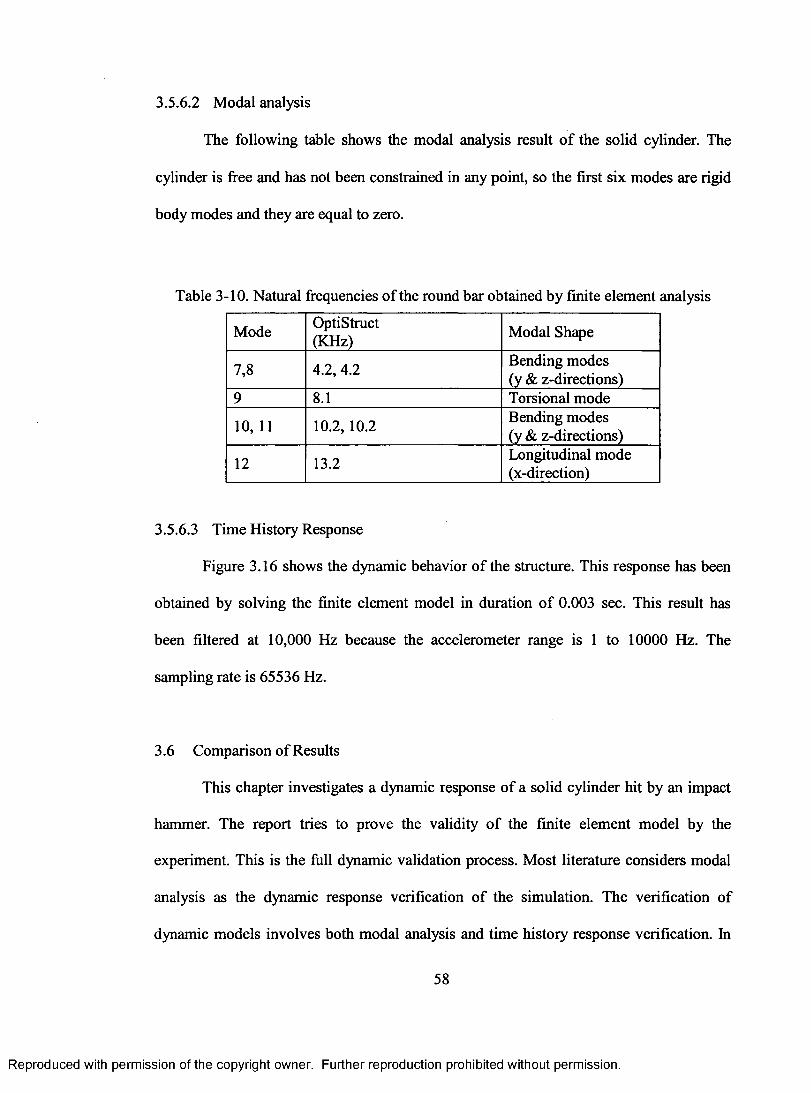
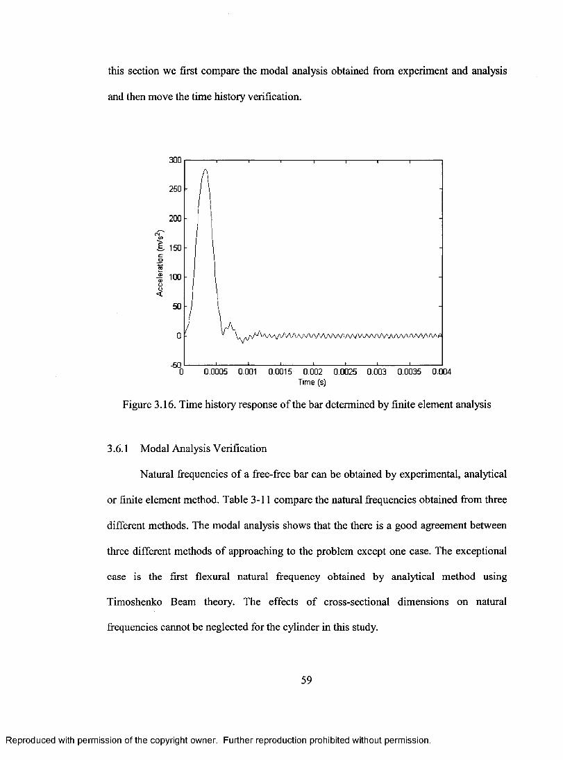
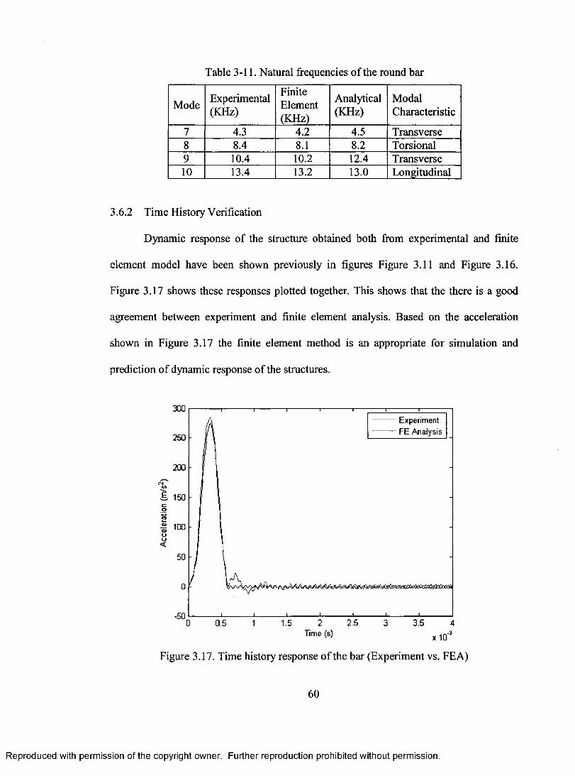
Page 1
UNLV Retrospective Theses & Dissertations
1-1-2007
Experimental and finite element studies of shock transmission Experimental and finite element studies of shock transmission
through bolted joints through bolted joints
Masoud Feghhi University of Nevada, Las Vegas
Follow this and additional works at: https://digitalscholarship.unlv.edu/rtds
Repository Citation Repository Citation Feghhi, Masoud, "Experimental and finite element studies of shock transmission through bolted joints" (2007). UNLV Retrospective Theses & Dissertations. 2765. http://dx.doi.org/10.25669/3r6f-f7ma
This Dissertation is protected by copyright and/or related rights. It has been brought to you by Digital Scholarship@UNLV with permission from the rights-holder(s). You are free to use this Dissertation in any way that is permitted by the copyright and related rights legislation that applies to your use. For other uses you need to obtain permission from the rights-holder(s) directly, unless additional rights are indicated by a Creative Commons license in the record and/or on the work itself. This Dissertation has been accepted for inclusion in UNLV Retrospective Theses & Dissertations by an authorized administrator of Digital Scholarship@UNLV. For more information, please contact [email protected] .
Page 2
EXPERIMENTAL AND FINITE ELEMENT STUDIES OF SHOCK TRANSMISSION
THROUGH BOLTED JOINTS
by
Masoud Feghhi
A dissertation submitted in partial fulfillment o f the requirements for the
Doctor of Philosophy Degree in Mechanical Engineering Department of Mechanical Engineering
Howard R. Hughes College of Engineering
Graduate College University of Nevada, Las Vegas
December 2007
Reproduced with permission of the copyright owner. Further reproduction prohibited without permission.
Page 3
UMI Number: 3302352
INFORMATION TO USERS
The quality of this reproduction is dependent upon the quality of the copy
submitted. Broken or indistinct print, colored or poor quality illustrations and
photographs, print bleed-through, substandard margins, and improper
alignment can adversely affect reproduction.
In the unlikely event that the author did not send a complete manuscript
and there are missing pages, these will be noted. Also, if unauthorized
copyright material had to be removed, a note will indicate the deletion.
UMIUMI Microform 3302352
Copyright 2008 by ProQuest LLC.
All rights reserved. This microform edition is protected against
unauthorized copying under Title 17, United States Code.
ProQuest LLC 789 E. Eisenhower Parkway
PC Box 1346 Ann Arbor, Ml 48106-1346
Reproduced with permission of the copyright owner. Further reproduction prohibited without permission.
Page 4
Dissertation ApprovalThe Graduate College University of Nevada, Las Vegas
18 October 20 07
The Dissertation prepared by
Masoud F egh h i__________
Entitled
E x p e r im en ta l and F i n i t e E lem en t S t u d ie s o f Shock T r a n sm iss io n Through
R o lle d J o i n t s
is approved in partial fulfillment of the requirements for the degree of
Ph.D . in M e ch a n ica l E n g in e e r in g _________________________
Exam ination C om m ittee M en-per
Examination C h m m ttee Mfimhei
Graduate College E aculty Representative
Exam ination C om m ittee Chair
Dean o f the Graduate College
/
Examination Committee Metmer
Reproduced with permission of the copyright owner. Further reproduction prohibited without permission.
Page 5
ABSTRACT
Experimental and Finite Element Studies of Shock Transmission Through Bolted Joints
by
Masoud Feghhi
Dr. Brendan J. O ’Toole, Examination Committee Chair Associate Professor o f Mechanical Engineering
University o f Nevada, Las Vegas
The aim o f this study is to analyze and assess the dynamic behavior o f bolted joint
connections subjected to impact loads using Finite Element Analysis (FEA) and
experiment. Also, it investigates the effect o f the joint on shock propagation through the
structure. There is little or no literature available describing the proper method for
analyzing the transient shock propagation across bolted connections. The main study will
be performed on hat sections bolted to a flat plate. These simple configurations are
representative o f structures found in many military ground vehicles that can be subjected
to transient impact and blast loads. The best way to approach this problem is first to
compare and verify the experiment and modeling results on the plate and hat section
individually. The next step is to verify the result o f a bolted structure. The last step would
be a parametric study o f the bolted joints with different variables, such as contact type
and area, friction, preload on bolt. Vibration characteristics o f bolt and spacers and FEA
results output frequency.
I l l
Reproduced with permission of the copyright owner. Further reproduction prohibited without permission.
Page 6
An impulse hammer with built in load cell along with accelerometers have been
used to obtain the response o f the shock for the experimental work. Finite element
Method (FEM) is used for analysis. The model has been made and meshed in
HyperMesh®, and then exported to LS-DYNA to solve and obtain the results from the
shock applied to the structure.
The results will be presented in three categories. First the modal analysis is
performed both numerically and experimentally. The results were in excellent agreement
with less than 2% error. Secondly, the time history response o f FEA and experimental
results are compared together. Different methods such as Root Mean Square (RMS),
moment method and maximum peak acceleration method was used to obtain the
resemblance o f experimental and Finite Element responses. The results show that solid
elements with a fine mesh must be used in the modeling the structure to obtain a reliable
response from FEA. Finally, the Shock Response Spectrum (SRS) is used to calculate the
critical frequency for design purposes. As long as the structure is modeled with the solid
elements and mesh is refined properly the FEA and experiment detects the same critical
frequency.
The study o f shock propagation through structure with bolted joints showed that
joint is reducing the maximum acceleration amplitude by a factor o f 3. Furthermore,
using a washer and bolt with a lower stiffriess material can attenuate shock significantly.
In some cases there is up to 40% reduction in peak acceleration.
IV
Reproduced with permission of the copyright owner. Further reproduction prohibited without permission.
Page 7
TABLE OF CONTENTS
ABSTRACT.................................................................................................................................. iii
LIST OF FIGURES.................................................................................................................... vii
LIST OF TABLES.........................................................................................................................x
NOMENCLATURE.................................................................................................................... xi
ACKNOWLEDGEMENTS......................................................................................................xiii
CHAPTER 1 INTRODUCTION............................................................................................. I1.1 Proj ect Overview............................................................................................................. 11.2 Application......................................................................................................................21.3 Problem Configuration....................................................................................................31.4 Review of Literature........................................................................................................61.5 Dissertation Objectives............................ 10
CHAPTER 2 COMPARISON OF TWO TRANSIENT RESPONSES...........................122.1 The Need for Establishing Error Criteria......................................................................122.2 Applications................................................................................................................... 142.3 Error Criteria Objectives............................................................................................... 162.4 Review of the Literature in Transient Response Comparison.......................................172.5 Error Calculation Methods............................................................................................ 192.6 Summary of Error Calculation Methods.......................................................................322.7 The Dissimilarity Factor (DF).......................................................................................34
CHAPTER 3 EXPERIMENTAL CALIBRATION OF FEA ............................................ 353.1 Introduction................................................................................................................... 353.2 Geometry of the Bar......................................................................................................353.3 Experimental Procedure................................................................................................363.4 Natural Modes of Vibration...........................................................................................473.5 Finite Element Analysis of a Simple Structure.............................................................533.6 Comparison of Results..................................................................................................58
CHAPTER 4 STRUCTURES WITHOUT JOINTS............................................................624.1 Introduction.............................................................,...................................................... 624.2 Quarter Inch Steel Plate.................................................................................................624.3 Hat Section.................................................................................................................... 834.4 Reflection of the Shock Wave..................................................................................... 102
Reproduced witti permission of ttie copyrigfit owner. Furtfier reproduction profiibited witfiout permission.
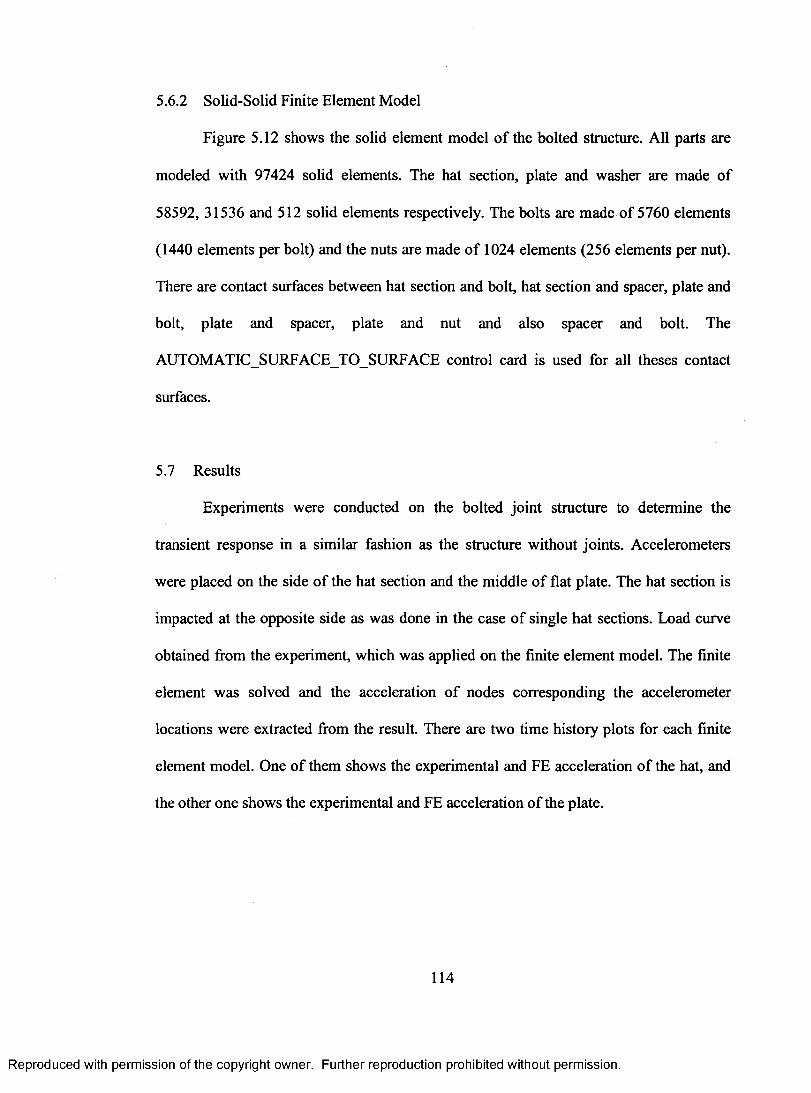
Page 8
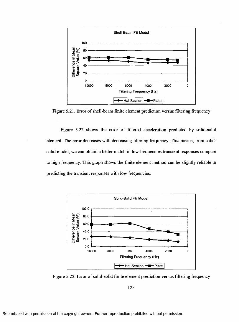
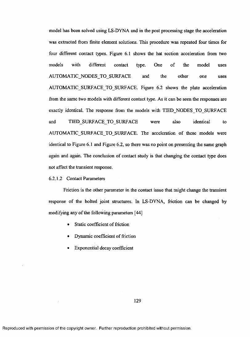
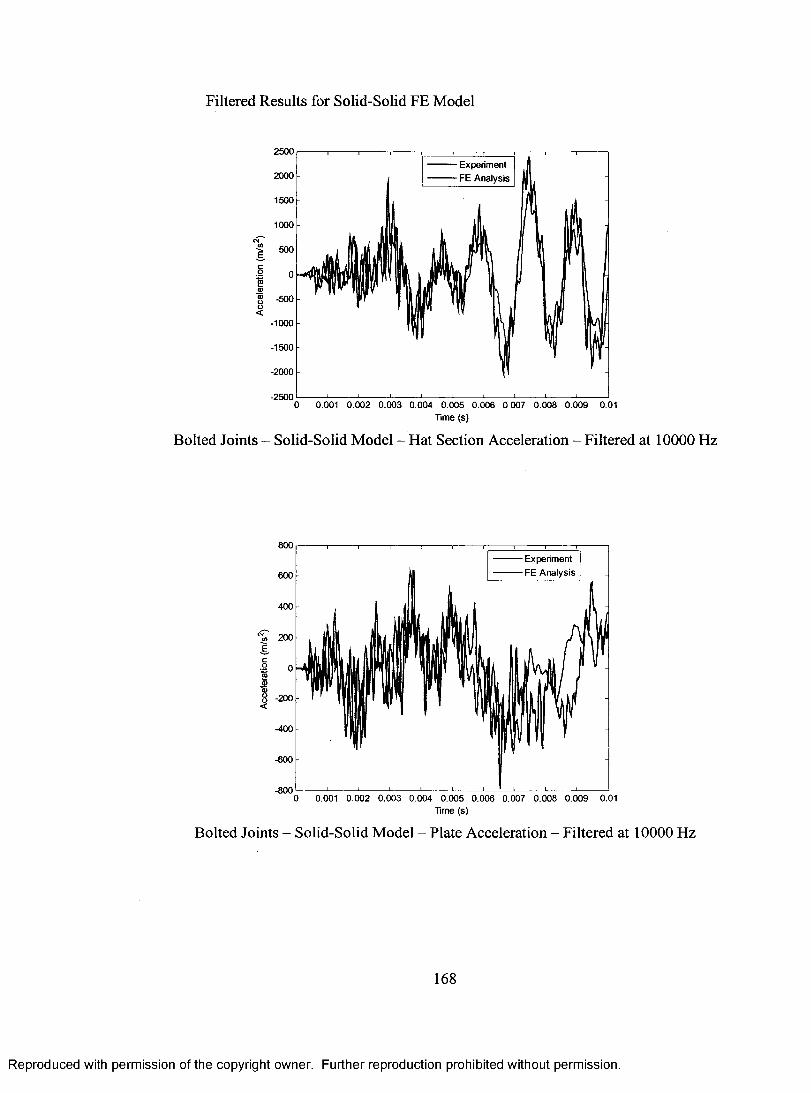
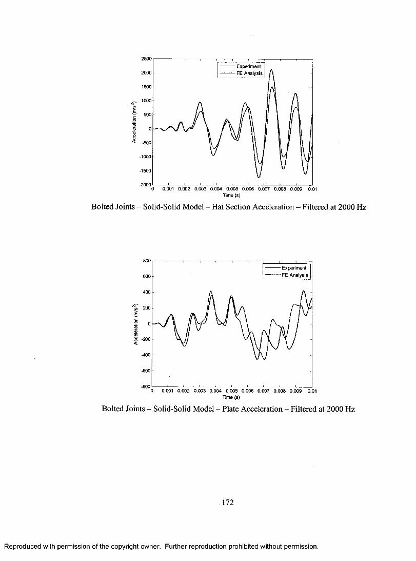
CHAPTER 5 SHOCK TRANSMISSION THROUGH THE BOLTED JOINTS......... 1045.1 Introduction................................................................................................................. 1045.2 Geometry and Dimensions of the Structure................................................................ 1055.3 Material Properties...................................................................................................... 1085.4 Appropriate Bolt Size.................................................................................................. 1085.5 Experiment.................................................................................................................. 1085.6 Finite Element Analysis.............................................................................................. I l l5.7 Results......................................................................................................................... 1145.8 Filtering the High Frequency....................................................................................... 1225.9 The Effect of Bolted Joints on Shock Mitigation........................................................ 124
CHAPTER 6 FINITE ELEMENT ANALYSIS OF JOINT PERFORM ANCE........... 1266.1 Introduction................................................................................................................. 1266.2 Parameters Effecting the Simulation........................................................................... 1266.3 Effect of the Joint in Shock Transmission Through the Structure...............................1406.4 Discretization of Finite Element Response ......................................................... 1506.5 Summary......................................................................................................................154
CHAPTER 7 SUMMARY, CONCLUSIONS, AND RECOMMENDATIONS.......... 1557.1 Summary......................................................................................................................1557.2 Conclusions................................................................................................................. 1577.3 Future Work................................................................................................................ 161
APPENDIX................................................................................................................................. 163
REFERENCES...........................................................................................................................173
VITA............................................................................................................................................180
VI
Reproduced with permission of the copyright owner. Further reproduction prohibited without permission.
Page 9
LIST OF FIGURES
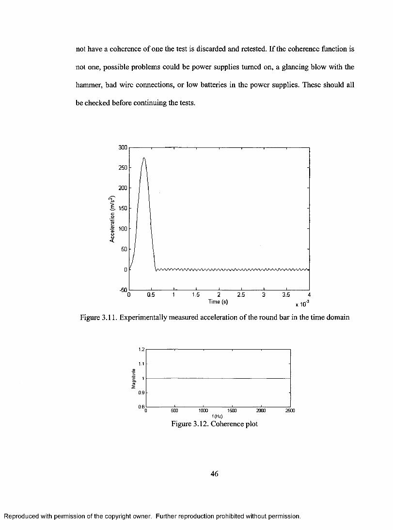
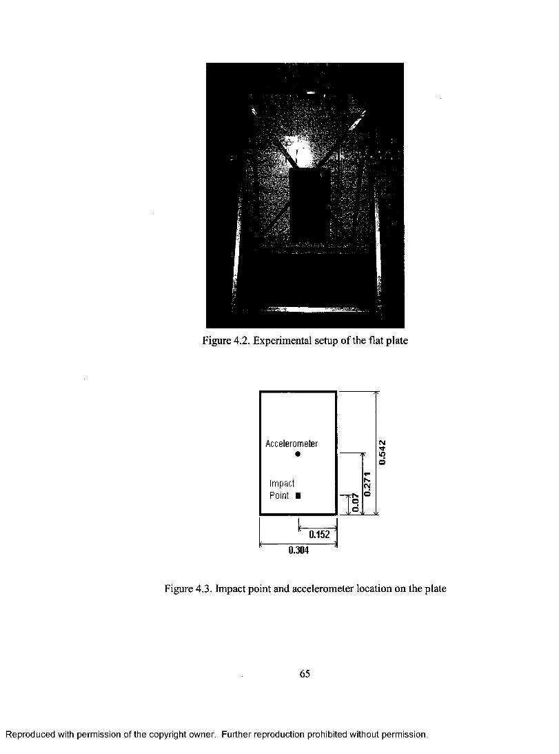
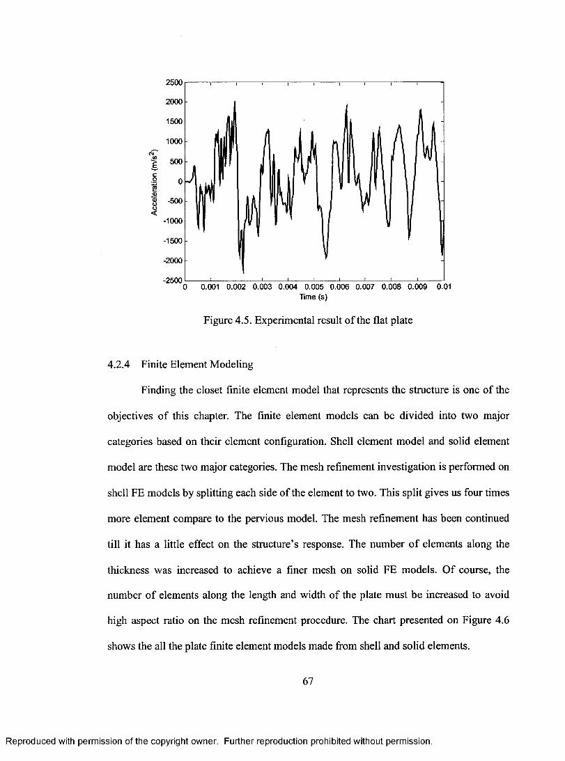
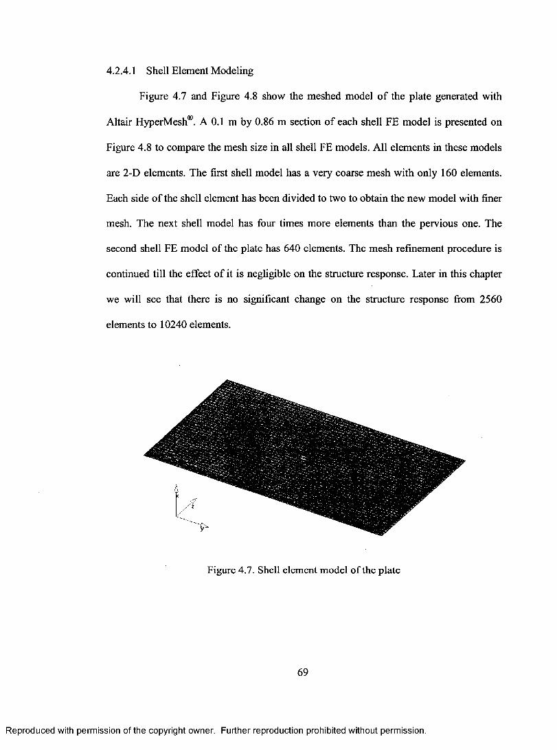
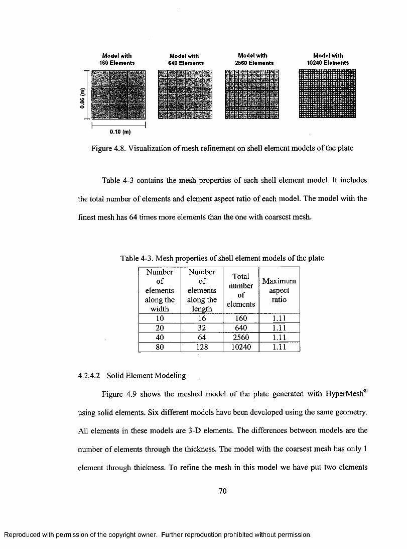
Figure 1.1. Dingo armored vehicle............................................................................................4Figure 1.2. The simplified model of the armored vehicle..........................................................5Figure 2.1. A typical result of a shock response of a structure from the experiment 12Figure 2.2. Shell element model and experimental results.......................................................13Figure 2.3. Solid element model and experimental results.......................................................14Figure 2.4. Seven days forecast and recorded temperature from Fox News [25]................... 15Figure 2.5. Seven days forecast and recorded temperature from Weather Channel [26]........16Figure 2.6. Illustration of the problem with two sets of analysis and experimental curves... 17Figure 2.7. Accelerations obtained from experimental results and shell FE model............... 20Figure 2.8. Error calculated with the regular method.............................................................. 21Figure 2.9. Two sets of curves with the same amplitude and same phase shift.......................23Figure 2.10. Example of curves with positive and negative skewness......................................26Figure 2.11. Example of curves with kurtosis greater and less than 3.......................................27Figure 2.12. Illustration of maximum peak error calculation method....................................... 30Figure 2.13. Comparison of two accelerations with peak counting method..............................32Figure 3.1. Dimensions of the Bar........................................................................................... 36Figure 3.2. PCB 086C02 impulse hammer (Small).................................................................37Figure 3.3. PCB 086C20 impulse hammer (Large).................................................................37Figure 3.4. Comparison of Large and small impulse hammers...............................................38Figure 3.5. PCB 352C22 ceramic shear ICP accelerometer....................................................38Figure 3.6. PCB 394C06 hand held calibrator.........................................................................40Figure 3.7. A six FFT input channel Pulse data acquisition hardware....................................41Figure 3.8. A-ffame and pendulum setup................................................................................43Figure 3.9. Experimental FFT plot of the round bar................................................................44Figure 3.10. Applied force measured by small impulse hammer to the round bar................... 45Figure 3.11. Experimentally measured acceleration of the round bar in the time domain 46Figure 3.12. Coherence plot....................................................................................................... 46Figure 3.13. Force curve applied to the finite element models..................................................55Figure 3.14. Impact point and accelerometers locations on hat section....................................56Figure 3.15. Solid element model of the round bar................................................................... 57Figure 3.16. Time history response of the bar determined by finite element analysis 59Figure 3.17. Time history response of the bar (Experiment vs. FEA).......................................60Figure 3.18. SRS of experimental and FE analysis of the bar................................................... 61Figure 4.1. Dimensions of the flat plate m m ........................................................................... 63Figure 4.2. Experimental setup of the flat plate....................................................................... 65Figure 4.3. Impact point and accelerometer location on the plate...........................................65Figure 4.4. Applied force to the flat plate measured by the instrumented hammer................ 66Figure 4.5. Experimental result of the flat plate...................................................................... 67Figure 4.6. Study of mesh refinement on plate finite analysis.................................................68Figure 4.7. Shell element model of the plate........................................................................... 69Figure 4.8. Visualization of mesh refinement on shell element models of the plate 70Figure 4.9. Solid element model of the plate.................... 71Figure 4.10. Mode shapes of the plate obtained by the finite elements modal analysis 74
vii
Reproduced with permission of the copyright owner. Further reproduction prohibited without permission.
Page 10
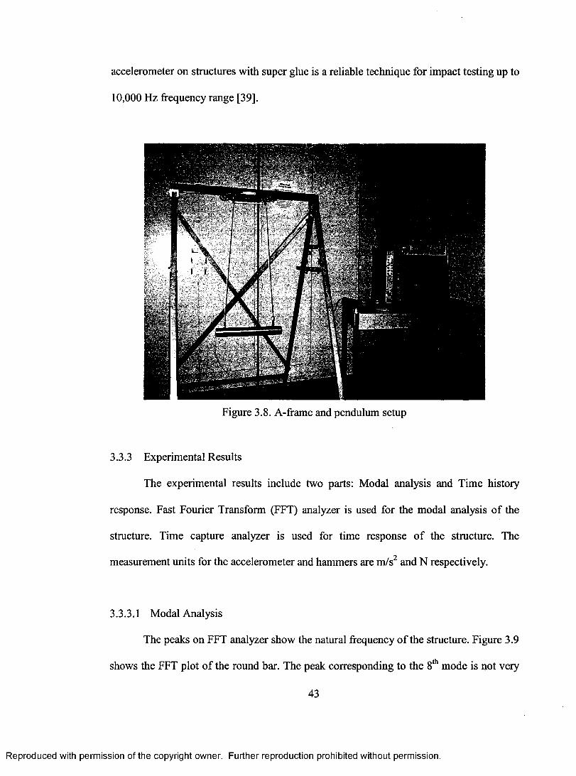
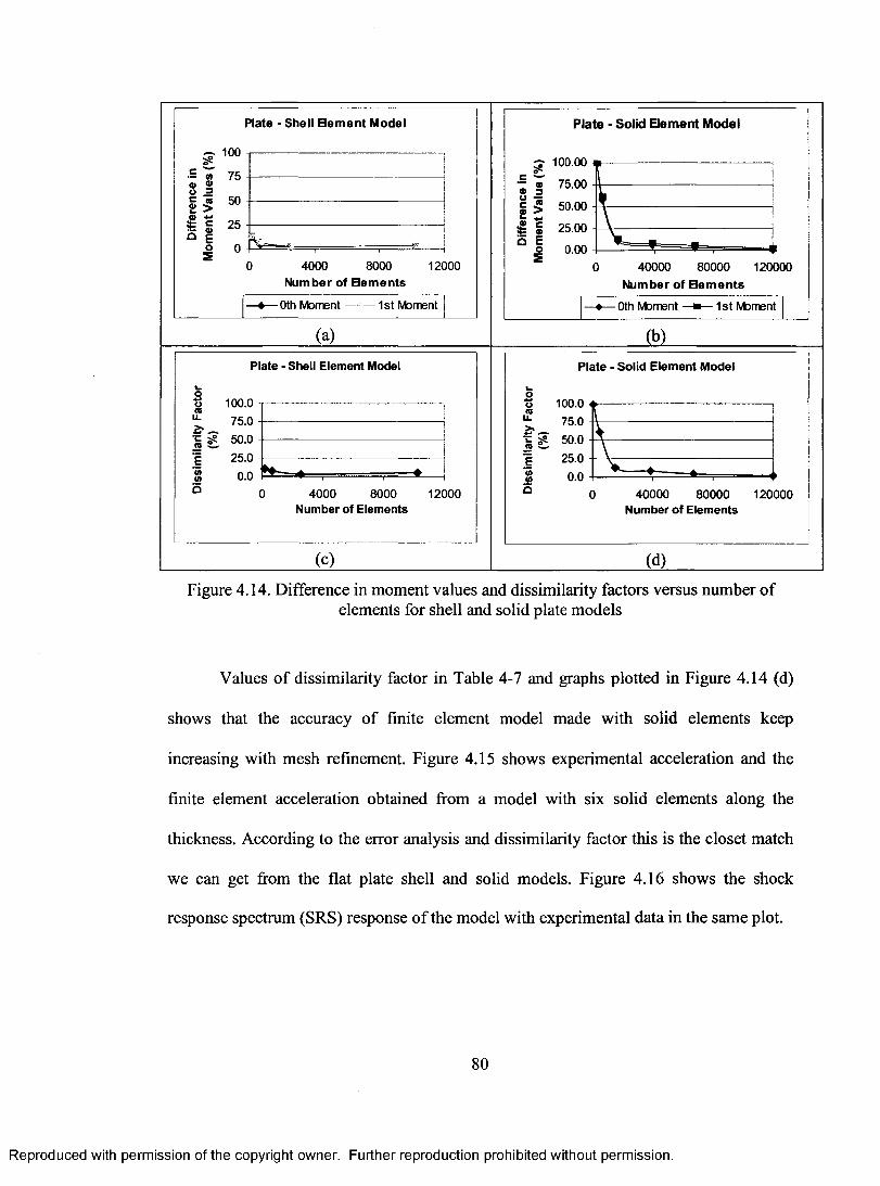
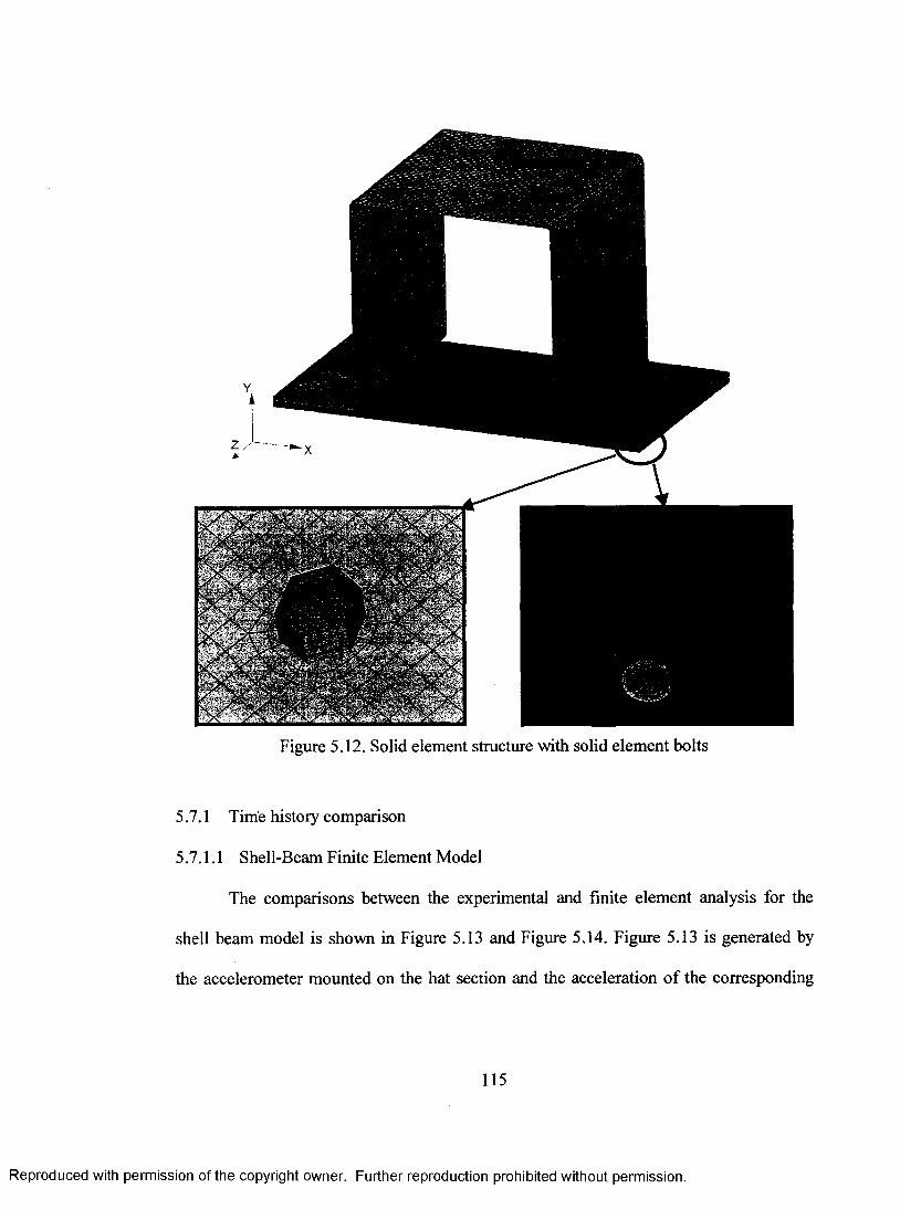
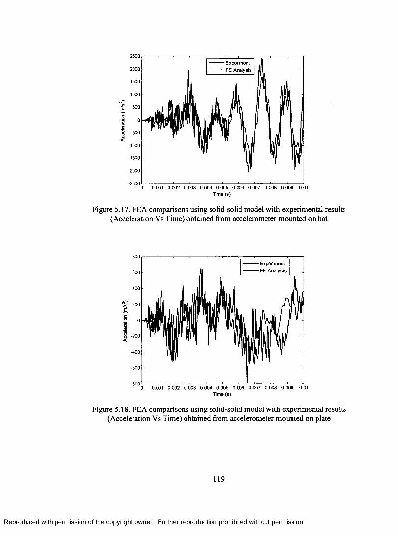
Figure 4.11. Time history response of the plate: Experimental and FE analysis model 75Figure 4.12. Shock response spectrum (SRS) of the plate: (shell element model)....................77Figure 4.13. Time history response of the plate: Experimental and FE analysis......................78Figure 4.14. Difference in moment values and dissimilarity factors for plate models..............80Figure 4.15. Time history response of the plate: Experimental and FE analysis..................... 81Figure 4.16. Shock response spectrum (SRS) of the plate: (solid element model)....................82Figure 4.17. Hat section configuration and dimensions are in m ..............................................83Figure 4.18. Experimental setup for hat section........................................................................84Figure 4.19. Hat section, accelerometers and large impact hammer.........................................85Figure 4.20. Impact point and accelerometer location on the hat section..................................85Figure 4.21. Applied force to the hat section by large instrumented hammer.......................... 86Figure 4.22. Experimental result of the hat section...................................................................87Figure 4.23. Study of mesh refinement on finite element modeling..........................................88Figure 4.24. Shell element model of a hat section configuration..............................................89Figure 4.25. Close up of part of shell element model of steel hat section.................................89Figure 4.26. Solid element model of a hat section configuration..............................................91Figure 4.27. Mode shapes of the hat section obtained by the FE modal analysis..................... 94Figure 4.28. Time history response of the hat section: Experimental and FEA....................... 95Figure 4.29. Shock response spectrum (SRS) of the hat section: (shell element model)......... 96Figure 4.30. Time history response of the hat section: Experimental and FEA....................... 97Figure 4.31. Difference in moment values and dissimilarity factors for hat section models... 99Figure 4.32. Time history response of the hat section: Experimental and FEA......................100Figure 4.33. Shock response spectrum (SRS) of the hat section: (solid element model) 101Figure 5.1 Assembly drawing of the bolted joint structure.................................................. 105Figure 5.2. Hat section configuration (dimensions are in mm).............................................106Figure 5.3. Plain washer, narrow, steel, zinc plated (dimensions are in mm)........................106Figure 5.4. Flat plate (dimensions are in mm)....................................................................... 107Figure 5.5. MlOx 1.25, class 8.8, hex bolt (dimensions are in mm )......................................107Figure 5.6. Bolted joint experimental setup........................................................................... 109Figure 5.7. Hat section and plate connected together with bolts...........................................109Figure 5.8. The location of accelerometers.......................................................................... 110Figure 5.9. Force curve applied to the finite element models................................................ I l lFigure 5.10. Finite element modeling of the bolted joint structure....................................... 112Figure 5.11. Shell element structure with beam element bolts................................................113Figure 5.12. Solid element structure with solid element bolts................................................. 115Figure 5.13. FEA comparisons using hat shell-beam model with experimental results 116Figure 5.14. FEA comparisons using plate shell-beam model with experimental results 116Figure 5.15. FEA comparisons of hat section with experimental results (SRS)....................117Figure 5.16. FEA comparisons of plate with experimental results (SRS)...............................118Figure 5.17. FEA comparisons using hat solid-solid model with experimental results 119Figure 5.18. FEA comparisons using plate solid-solid model with experimental results 119Figure 5.19. FEA comparisons of hat section with experimental results(SRS)...................... 120Figure 5.20. FEA comparisons of plate solid-solid model with experimental results (SRS) 120Figure 5.21. Error of shell-beam finite element prediction versus filtering frequency 123Figure 5.22. Error of solid-solid finite element prediction versus filtering frequency 123Figure 5.23. Experimental time history response of the (a) hat section and (b) plate 124Figure 5.24. Experimental SRS of the (a) hat section and (b) plate........................................125Figure 6.1. Acceleration of the hat section (different contacts).............................................130Figure 6.2. Acceleration of the plate (different contacts)......................................................130Figure 6.3 . Hat section acceleration plots (different friction coefficients)............................132Figure 6.4. Plate acceleration plots (different friction coefficients)......................................132
viii
Reproduced with permission of the copyright owner. Further reproduction prohibited without permission.
Page 11
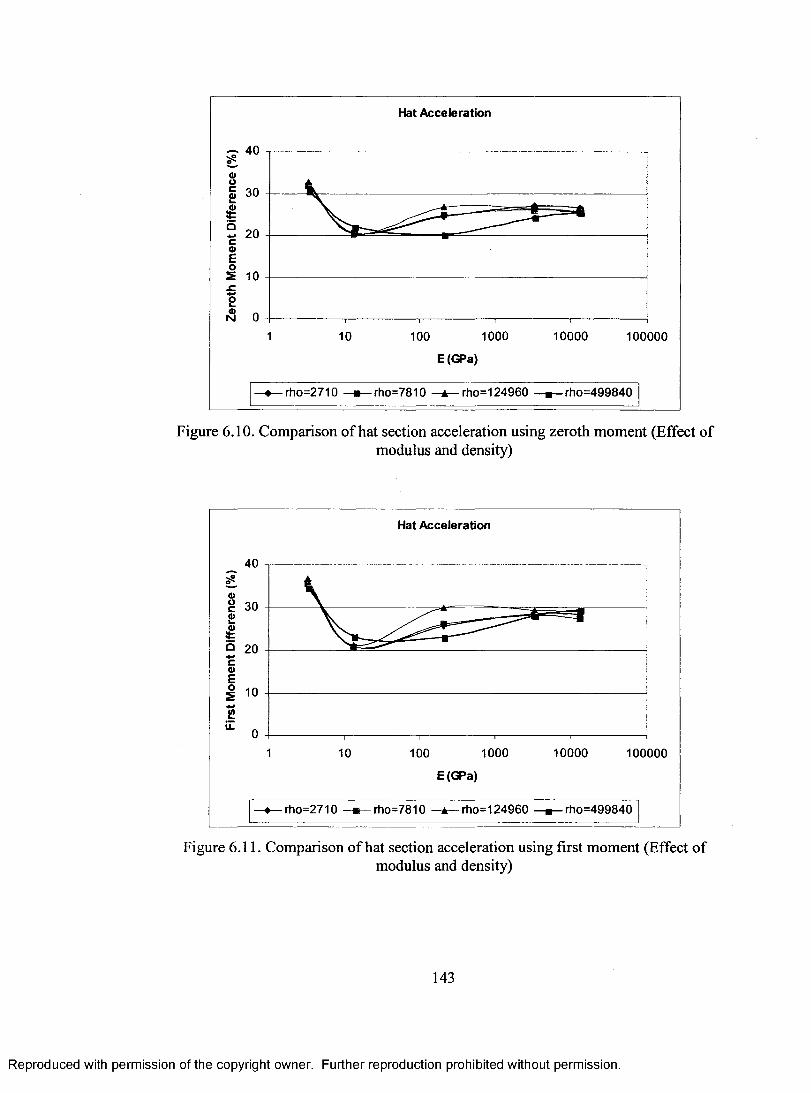
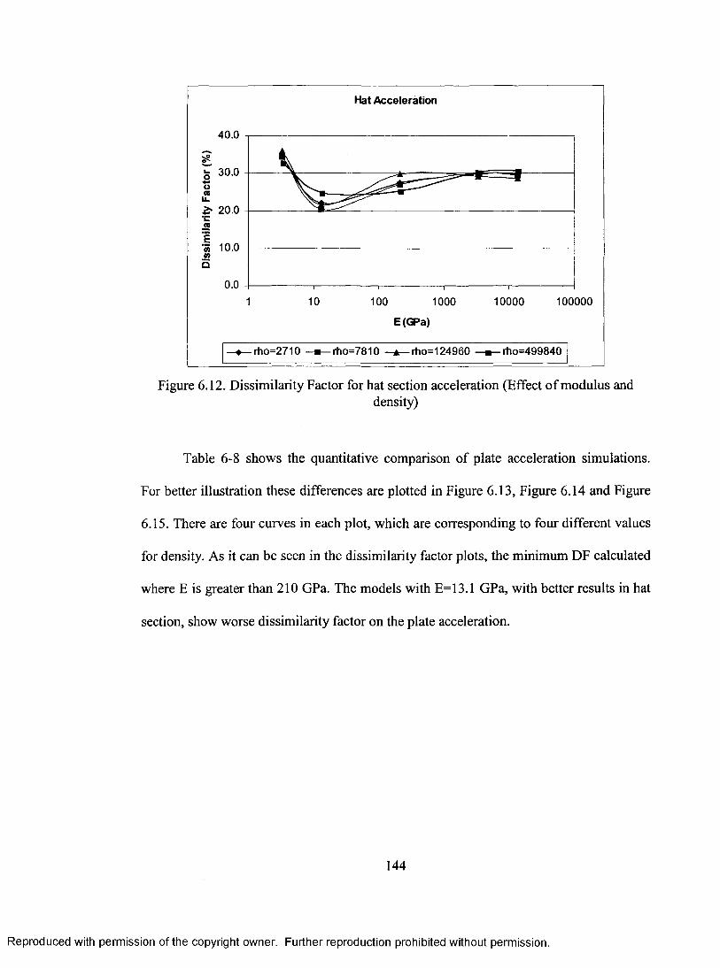
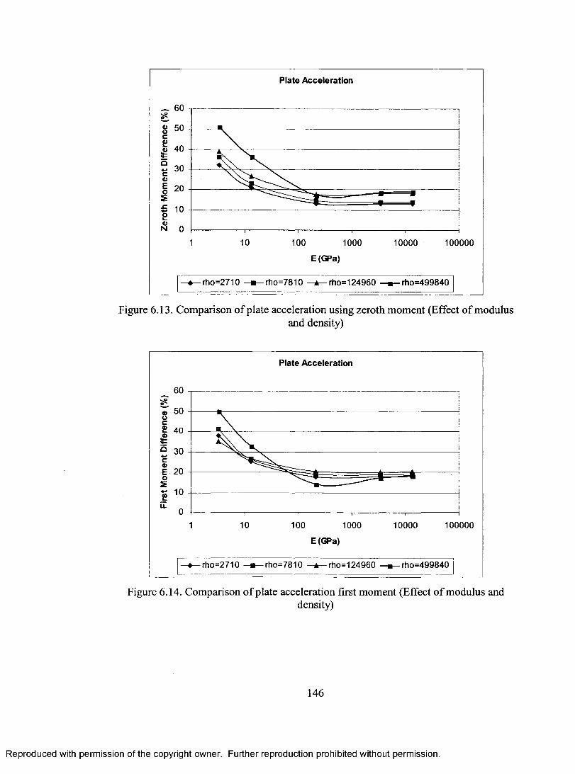
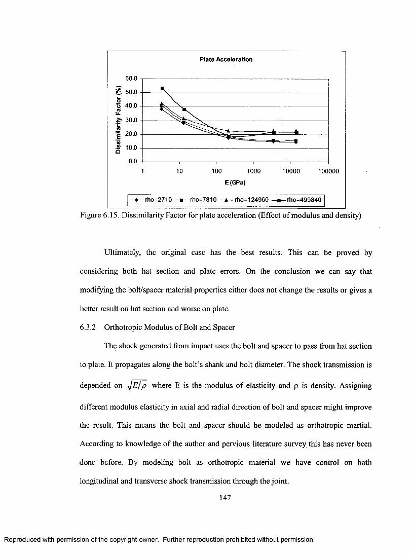
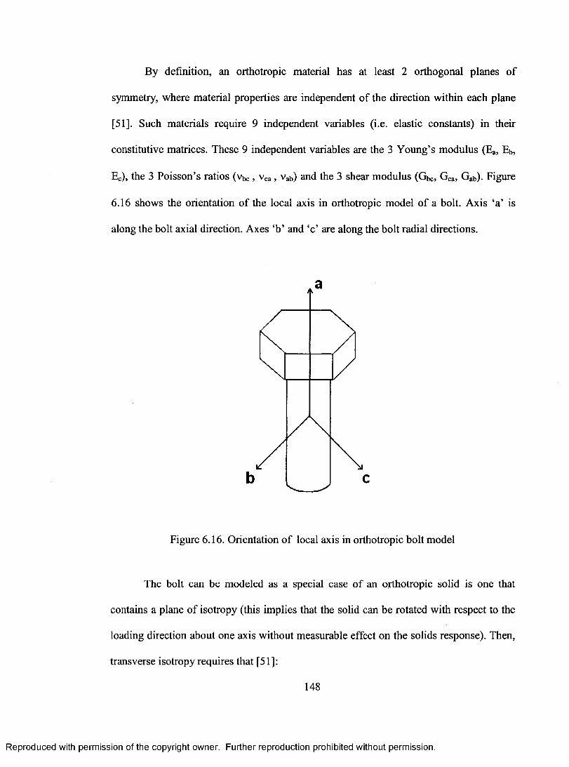
Figure 6.5. Structure showing the constant pre-stress of 460 M Pa....................................... 135Figure 6.6. FFT of hat section for 100, 75 and 21Nm Torque............................................... 136Figure 6.7. Time History response on the structure...............................................................137Figure 6.8. Hat accelerations - results output frequency.......................................................139Figure 6.9. Plate acceleration - results output frequency......................................................139Figure 6.10. Comparison of hat section acceleration using zeroth moment (E & p) 143Figure 6.11. Comparison of hat section acceleration using first moment (E & p )................. 143Figure 6.12. Dissimilarity Factor for hat section acceleration (E & p ) ...................................144Figure 6.13. Comparison of plate acceleration using zeroth moment (E & p )....................... 146Figure 6.14. Comparison of plate acceleration first moment (E & p ).....................................146Figure 6.15. Dissimilarity Factor for plate acceleration (E & p).............................................147Figure 6.16. Orientation of local axis in orthotropic bolt model............................................148Figure 6.17. Hat section acceleration versus time obtained from experiment and FEA 151Figure 6.18. Plate acceleration versus time obtained from experiment and FEA.................... 151Figure 6.19. Hat section dissimilarity factor versus time span.............................................. 153Figure 6.20. Plate dissimilarity factor versus time span..........................................................153
IX
Reproduced with permission of the copyright owner. Further reproduction prohibited without permission.
Page 12
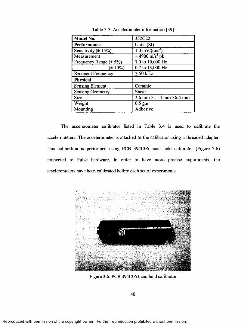
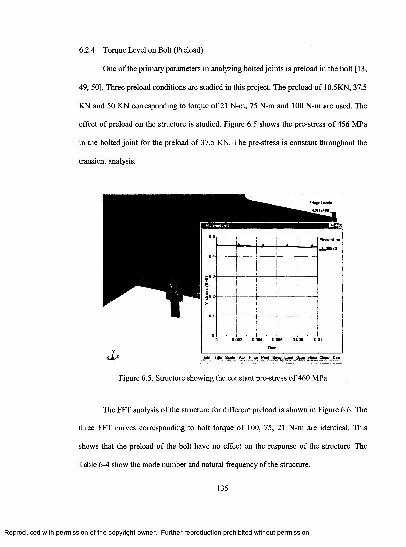
LIST OF TABLES
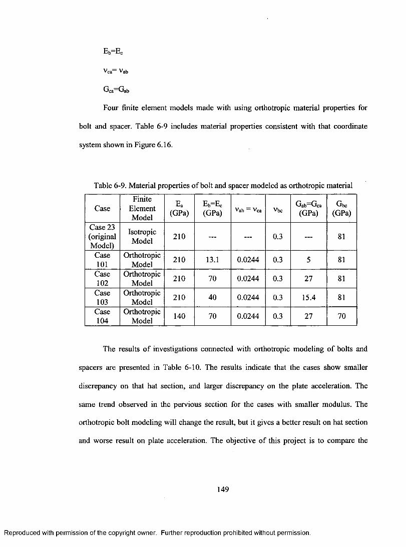
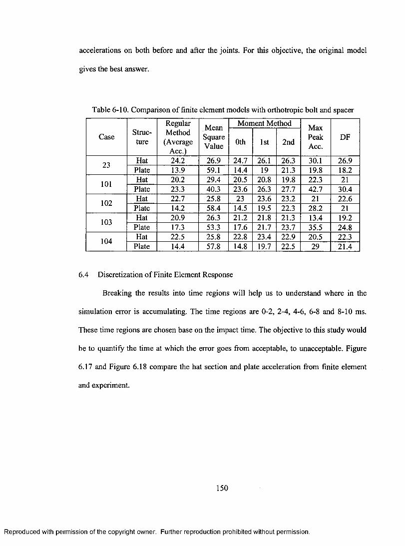
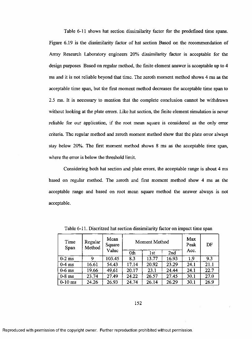
Table 3-1. PCB 086C02 Modally Tuned Impulse Hammer...................................................39Table 3-2. PCB 086C20 Modally Tuned Impulse Hammer...................................................39Table 3-3. Accelerometer information....................................................................................40Table 3-4. Accelerometer Calibrator information..................................................................41Table 3-5. Pulse data acquisition hardware information........................................................42Table 3-6. Experimental natural frequencies of the round bar...............................................44Table 3-7. Analytical natural frequencies of the round bar....................................................52Table 3-8. Units used in the Modeling Analysis....................................................................54Table 3-9. Material properties of cold roll steel.....................................................................54Table 3-10. Natural frequencies of the round bar obtained by finite element analysis 58Table 3-11. Natural frequencies of the round bar.....................................................................60Table 3-12. Experiment and FEA comparison of the solid cylinder........................................61Table 4-1. Units on the experiment and analysis....................................................................63Table 4-2. Material properties of ASTM-A36 steel................................................................64Table 4-3. Mesh properties of shell element models of the plate...........................................70Table 4-4. Mesh properties of solid element models of the plate...........................................72Table 4-5. Modal analysis result of the plate..........................................................................73Table 4-6. Comparison of the plate experiment and FE shell model......................................76Table 4-7. Comparison of the plate experiment and FE solid model.....................................79Table 4-8. Mesh properties of shell element models of the hat section................................. 90Table 4-9. Mesh properties of solid element models of the hat section................................. 91Table 4-10. Modal analysis of hat section................................................................................93Table 4-11. Error analysis of the time domain response of the hat section shell model 95Table 4-12. Error analysis of the time domain response of the hat section solid model 98Table 5-1. Mechanical properties of the bolted joint parts................................................... 108Table 5-2. Transient response comparison for bolted joint structure...................................121Table 6-1. Comparison of experiment and FE model on bolted joint structure....................127Table 6-2. Coefficient of friction for steel surfaces............................................................. 131Table 6-3. Comparison of finite element models with different contact area.......................134Table 6-4. Natural frequency of structure............................................................................. 136Table 6-5. Simulation time step for finite element model.................................................... 138Table 6-6. Modulus and density of the bolt/spacer............................................................... 141Table 6-7. Comparison of Hat section acceleration(bolt/spacer material properties) 142Table 6-8. Comparison of plate acceleration (bolt/spacer material properties)....................145Table 6-9. Material properties of bolt and spacer modeled as orthotropic material 149Table 6-10. Comparison of finite element models with orthotropic bolt and spacer 150Table 6-11. Discritzed hat section dissimilarity factor on impact time span..........................152Table 6-12. Discritzed plate dissimilarity factor on impact time span................................... 153
Reproduced with permission of the copyright owner. Further reproduction prohibited without permission.
Page 13
NOMENCLATURE
a Time location
A(t) Analysis result, data or curve (function o f time)
e The value o f the error
D Root mean square duration value
Mean square duration value
DF Dissimilarity Factor
E[ ] Expected value o f [ ]
E(t) Error signal; Error curve (function o f time)
f(x) Probability density function; pdf
K Kurtosis
mn The nth generalized moment
Mr The rth temporal moment.
Max [ ] Maximum value o f [ ]
N Sample size. Number o f sample records
Pr[ ] Probability of [ ]
s Sample standard deviation
s Sample variance
S Skewness
t Time variable
Var[ ] Variance o f [ ]
xi
Reproduced with permission of the copyright owner. Further reproduction prohibited without permission.
Page 14
X Random variable
X Sample mean
X(t) Experimental result, signal, data or eurve (function o f time). Time History
response
|[ ]| Absolute value o f [ ]
a Arbitrary point as tbe origin o f tbe moment
X, Time bistory energy
p Population mean; Mean value
Pn Central moments
Raw moments
o Standard deviation
Variance
S [ ] Summation o f [ ]
X Centroid
Y Root mean square value
Mean square value
XU
Reproduced with permission of the copyright owner. Further reproduction prohibited without permission.
Page 15
ACKNOWLEDGEMENTS
The author is truly grateful to his advisor Dr. Brendan J. O ’Toole, the Committee
Chair Person for his guidance and encouragement throughout this investigation.
Dr. Brendan J. O ’Toole has been an inspiration to me in both academic and personal life.
I would also like to thank Mr. Kumarswamy Karpanan whose suggestions and advices
have been great help for me. Kumar is an individual with drive; be is a dedicated
engineer and a great friend and colleague.
Tbe author wishes to express bis sincere thanks and heartiest gratitude to Dr.
Samaan Ladkany, Dr. Woosoon Yim , Dr. Samir Moujaes and Dr. Douglas Reynolds for
their time in reviewing the prospectus, participation o f defense, and counseling o f the
thesis as the committee members.
I would like to thank my father, Mr. Abdollah Feghhi, and remember my beloved
mother. What I owe them cannot be described by words. They have given me everything.
Let it be known, this dissertation, every work I have ever done, and every work I will
ever do is solely dedicated to my father and mother.
The financial support provided by the Army Research laboratory (ARL), under
project BS3 is thankfully acknowledged.
The author expresses his thanks to the support and help o f my friends and
colleagues through out this investigation.
Xlll
Reproduced with permission of the copyright owner. Further reproduction prohibited without permission.
Page 16
CHAPTER 1
INTRODUCTION
1.1 Project Overview
It has been a while since scientists first started investigating different methods to
find the response o f a joint to an impact or shock. The finite element method has been
very useful in the simulation o f mechanical joints behavior. The finite element method is
a powerful computer based mathematical analysis and design tool, which emerged with
the advent o f the high speed digital computer. Its development was pioneered during the
1950's and 1960's by structural engineers working in the aerospace industry. Since then it
has been widely used for modeling and simulation o f different linear and nonlinear
problems, both static and dynamic in subjects o f structural analysis, fluid flow, heat
transfer, and fracture mechanics.
Mechanical joints, especially fasteners have a complex nonlinear behavior. The
finite element method seems to be the only option for simulating the transient response of
a joint under dynamic loading. Even this method has some limitations in simulating
dynamic response. This study investigates the dynamic response o f structures with and
without joints to suggest a simulation method with the most accurate response. The first
part o f this study focuses on structures without any joints. Simple structures like a beam
and a fiat plate are employed for the simulation proposes.
Reproduced with permission of the copyright owner. Further reproduction prohibited without permission.
Page 17
Most o f the time, simulation o f a system response is the only way to understand
the system behavior. There are many parameters to choose or ignore when it comes to
building a model for the simulation. Picking the right parameters leads to a reliable
simulation, and it is impossible to get an exact match between any simulation or analysis
and experimental data. The goal o f this work is to determine a satisfactory method for
analyzing shock propagation across bolted joints and to provide experimental guidelines
for verifying the analysis procedures.
1.2 Application
The main part o f this study will be performed on a steel hat section bolted to a flat
plate. These simple configurations are representative o f structures found in many military
ground vehicles that can be subjected to transient impact and blast loads. This is the main
application o f this project. In order to understand the response o f a structure, we must
have a good understanding o f its components. Joints are the key components of
structures. Almost every structure uses one or a mixture o f mechanical joints such as
welding, adhesive bonding and mechanical fasteners. Extensive research is in progress to
analyze the dynamic response o f complex structures involving assemblies, such as a light
combat vehicles. This study evaluates the structural integrity o f such structures when they
are subjected to transient loading [I].
Joints play a very important role in maintaining the structural integrity o f a
combat vehicle. Non-linear shock transfer performance o f joints has substantial influence
on the dynamics o f assembled structures as they induce a large amount o f damping into
the structure [2]. Study of shock transmission through the various jointed (both
Reproduced with permission of the copyright owner. Further reproduction prohibited without permission.
Page 18
mechanical and adhesive) components o f the comhat vehicle is o f particular interest to
the army. There is a need to guarantee the survivability and minimize the damage caused
to both the primary and secondary electronic systems present inside the combat vehicle.
Another area o f eoneem is to reduce or damp the shock transmission caused by a
projectile impact. On a armored vehicle, there is an immediate need to develop
methodologies for constructing predictive models o f structures with joints and shock
based dynamic response analysis in order to ensure the safety o f critical equipment and
hardware [3].
1.3 Problem Configuration
Many military systems must be capable o f sustained operation in the face o f
mechanical shocks due to projectile or other impacts. Many Army platforms (such as
vehicles) are made o f the chassis and top part, which are usually bolted together. Figure
1.1 shows the Dingo armored vehicle [4], which is made o f top part and chassis bolted
together. The vehicle consists o f several parts, which some o f them that can be clearly
seen are the tires, driver and commander doors (dome-shaped which open upwards),
latches, and connections. Several o f the components are joined together with bolts
through flanges. It is nearly impossible to model all the bolted connections with complete
detail because o f computational limitations
Reproduced with permission of the copyright owner. Further reproduction prohibited without permission.
Page 19
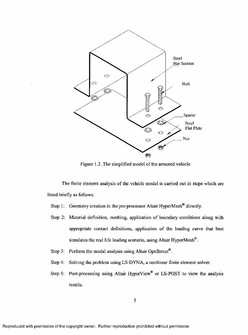
Figure 1.1. Dingo armored vehicle
It is important to understand the physical mechanism o f shock transfer through
bolted connections, so that simplified, but accurate modeling methods can be
incorporated into large vehicle design models. This dissertation focuses on developing an
understanding o f shock propagation through a bolted structure that is typical to a variety
o f military vehicle structures (Figure 1.2). The bolted hat section and plate structure (was
selected for study based on numerous discussions with structural dynamic research staff
at the U.S. Army Research Laboratory (ARL). Impact loads to this structure cause axial,
bending and shear shock loading through bolted connections.
Reproduced with permission of the copyright owner. Further reproduction prohibited without permission.
Page 20
SteelHat Section
Boit
©Spacer
Steel Fiat Plate
©Nut
Figure 1.2. The simplified model o f the armored vehicle
The finite element analysis o f the vehicle model is carried out in steps which are
listed briefly as follows.
Step 1 : Geometry creation in the pre-processor Altair HyperMesh® directly.
Step 2: Material definition, meshing, application o f boimdary conditions along with
appropriate contact definitions, application o f the loading eurve that best
simulates the real life loading scenario, using Altair HyperMesh®.
Step 3: Perform the modal analysis using Altair OptiStrcut®.
Step 4: Solving the problem using LS-DYNA, a nonlinear finite element solver.
Step 5: Post-processing using Altair HyperView® or LS-POST to view the analysis
results.
Reproduced with permission of the copyright owner. Further reproduction prohibited without permission.
Page 21
1.4 Review o f Literature
Little work has been published on the study o f shock transmission through jointed
structures; however there has been a great deal o f work done on both shock propagation
in structures and static analysis o f jointed structures. The design of structural systems
involves elements that are joined through bolts, rivets and pins. Joints and fasteners are
used to transmit loads from one structural element to another. In structures, there are
three types o f joints commonly used, namely, welded, mechanically fastened joints and
adhesive bonded joints. Fastened joints include bolts, rivets, and pins [3, 5].
Despite the adhesive joints being used for joining secondary structures, bolting
and welding are the main solution for joining the crucial structure parts. Nevertheless it
cannot be said that one particular type o f joint is better than the other as all the joints have
their own advantages. For instance adhesive bonding offers improved joint stiffness
compared to mechanical fasteners. An adhesive is essentially used for dual purposes, it
not only provides mechanical strength but it also seals the joint against moisture and
debris ingress [5].
The joint represents a discontinuity in the structure and results in high stresses
that often initiate structural failure [3]. The complex behavior o f connecting elements
plays an important role in the overall dynamic characteristics o f structures. This complex
behavior can be the effect o f slip in contact area around the bolted joints [6-9].
Detailed finite element models have been developed to establish an understanding
o f the slip-stick mechanism in the contact areas o f the bolted joints [6]. Bolted or riveted
joints are the primary source o f damping in the structure, because o f the friction in the
contact area [2]. The nonlinear transfer behavior o f the fiictional interfaces often provides
Reproduced with permission of the copyright owner. Further reproduction prohibited without permission.
Page 22
the dominant damping mechanism in jointed structure. They play an important role in the
vibration properties o f the structure [7].
Friction in bolted joints is one o f the sources o f energy dissipation in mechanical
systems. The finite element models are constructed in a nonlinear framework to simulate
the energy dissipation through joints [9]. Sandia National Laboratory also has an
extensive research program for investigating energy dissipation due to microslip in bolted
joints [8].
‘Preload’ and ‘mechanical clearance’ are two parameters that might effect the
dynamic behavior o f bolted joints. Most o f the research in the modeling o f preload has
been done for fatigue or cyclic loading. These kinds o f loads are usually in the category
o f the static loading, but because o f the importance o f these parameters it is useful to
mention them in dynamic response o f the joints. Duffey, Lewis and Bowers [10] present
two types o f pulse-loaded vessel closers to determine the influence o f bolt preload on the
peak response o f closure and bolting system. The effect o f bolt prestress on the maximum
bolt displacement and stress has been investigated by Esmalizedeh et al [11]. The loading
is assumed to be initially peaked, exponentially decaying internal pressure pulse acting
on the bolted closure. Kerekes [12] use a simple beam model o f the screw with fatigue
loading to show the damage vulnerability o f prestressed screws on the flange plate. In all
o f these studies there is no indication about how to apply the preload to the finite element
model. O ’Toole et al. [13] show several different preload modeling procedures for
dynamic finite element analysis and make recommendations on the most suitable
methods. Szwedowicz et al. [14] presented the modal analysis o f a pinned-elamped beam
for three different magnitudes. They have determined that even for fine meehanical fit
Reproduced with permission of the copyright owner. Further reproduction prohibited without permission.
Page 23
with the maximum bolt clearance up to 5 pm, the analytical and numerical
eigenfrequencies above the 2" mode show discrepancies with the measured results.
Zhange and Poirier [15] have developed a new analytical model o f bolted joints.
In this model, the member deformation is determined by the member stiffness that
remains unchanged whether the external load is present. They have used finite element
analysis to confirm the new model and observation. Song et al. [16, 17] have developed
an Adjusted Iwan Beam Element (AIBE), which can simulate the non-linear dynamic
behavior o f bolted joints in beam structures. The same element was used to replicate the
effects o f bolted joints on a vibrating frame; the attempt was to simulate the hysteretic
behavior o f bolted joints in the frame. The simulated and experimental impulsive
acceleration responses had good agreement validating the efficacy o f the AIBE. The
beam element developed is two-dimensional and consists o f two adjusted Iwan models
and maintains the usual complement o f degrees o f freedom: transverse displacement and
rotation at eaeh o f the two nodes. This element includes six unknown parameters. A
multi-layer feed-forward neural network is considered to obtain these parameters, from
measured acceleration responses. The experimental result has been used to validate the
simulated acceleration responses [17].
Different methods have been employed to determine the dynamic response o f
complex jointed structures. Studying the natural frequencies, modal behavior and
damping o f a structure, which constitute its dynamic characterization, gives us a better
understanding o f the dynamics o f a structure and its reliability [18]. The Frequency
Response Function (FRF), which is obtained from Fast Fourier transform (FFT), is the
widely used method for determining the natural frequencies and mode shapes o f a
8
Reproduced with permission of the copyright owner. Further reproduction prohibited without permission.
Page 24
structure [19]. Nevertheless it is possible to determine the natural frequencies o f a
structure using FFT; determining the conspicuous peaks in the FFT analysis does this, the
frequencies corresponding to these peaks are the natural frequencies o f the structure [20].
Responses measured from impulsive loading (like blast or impaet) are typically
accelerations, veloeities and displacements at the crucial locations on the structure. While
comparing the finite element results with the results obtained from experiments, one o f
these parameters is considered [21]. Little work has been published on presenting the
study o f shock transmission through jointed structures; however there has been a great
deal o f work done on both shock propagation in structures and jointed static analysis o f
joints.
A few finite element models for joints are being developed [22, 23] which can
predict the dynamic response for a particular application. Adoption o f this type of
analysis early in the design phase can influence decisions that improve the structural
performance. Crash modeling and simulation is one o f the subjects that finite element
analysis has been employed to obtain the dynamic response o f the whole structure,
including joints. A truck impacting a guardrail system is one o f the examples o f these
crash analyses [22]. In this study a spring has been used to simulate component
crashworthiness behavior, like the bolted connection between the rail and block-out.
For the safety o f the driver o f a delivery motor vehiele, a new concept of
breakaway mailbox support has been developed by Reid [23]. The new breakaway
concept consists o f modifying the material o f anchor bolt to have a higher strength and
lower percent elongation. Nonlinear finite element analysis with LS-DYNA was also
used to predict the potential for the new breakaway mount and attached mailbox to meet
Reproduced with permission of the copyright owner. Further reproduction prohibited without permission.
Page 25
the crash test requirements o f NCHRP Report No. 350 [24]. Most o f these research
efforts have followed the Federal Highway Administration (FHWA) safety performance
criteria. FHWA policy requires the use o f devices on the National Highway System that
have been suecessfully tested in accordance with the guidelines eontained in the National
Cooperative Highway Research Program (NCHRP) Report 350, “Recommended
Procedures for the Safety Performance Evaluation o f Highway Features”. The procedure
in ‘NCHERP report 350’ requires the use o f dynamic time history response to verify the
finite element simulation with experimental results [24].
Semke et al. [20] has analyzed the dynamic response o f a piping system with a
bolted flange. Experimental and numerical results are presented and show excellent
correlation. The experimental procedure utilizes an accelerometer to gather the dynamic
response output o f the piping system due to an impulse. The resonant frequencies are
then determined using a Fast Fourier Transform (FFT) method. The dynamic effects o f a
bolted flange and gasket on a piping system are critical in their use and it has been
demonstrated that the finite element method can simulate the response o f an overhanging
beam with a varying mid span.
1.5 Dissertation Objectives
The aim o f this study is to analyze and assess the dynamic behavior o f bolted joint
connections subjected to impact loads using finite element analysis. In other words, the
objective is to develop solutions that enable designers to generate improved physics-
based shock models for structures focusing mainly on shock transmission across
structural joints. The first step is to study the response o f individual components that
10
Reproduced with permission of the copyright owner. Further reproduction prohibited without permission.
Page 26
make up the bolted system. Transient analysis and experiments are performed on a flat
plate and a single hat section to benchmark both methodologies. Then similar analysis
and experiments are performed on an assembly with multiple joints.
The goal is to perform a detailed analysis o f a jointed structure that verifies a
response within 15 to 20 percents o f experimental data and shows quantitatively the
effect o f joint configuration on structural response. The following steps have been
employed and presented in the following chapters to study the response o f the jointed hat
section:
• Choosing a proper comparison factor to quantify the difference between time
histories.
• Perform FFT analysis on the structures without the joints and compare the natural
frequencies obtained from the finite element analysis.
• Perform impact experiments on the structures without the joints, which will
provide input data (force vs. time) and response data (aceeleration and/or strain
vs. time).
• Demonstrate that this experiment can be computationally simulated using a
detailed 3-D LS-DYNA analysis.
• Investigate the ability to accurately simulate the structural response for the
structures without joints
• Describe a simulation procedure, which obtains the most accurate dynamic
response o f a structure.
• Verify the simulation procedure on the geometrically nonlinear bolted joint
structures.
11
Reproduced with permission of the copyright owner. Further reproduction prohibited without permission.
Page 27
CHAPTER 2
COMPARISON OF TWO TRANSIENT RESPONSES
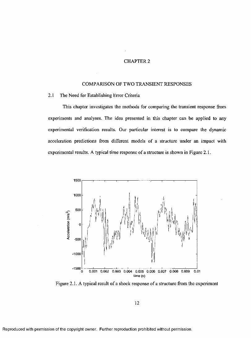
2.1 The Need for Establishing Error Criteria
This ehapter investigates the methods for comparing the transient response from
experiments and analyses. The idea presented in this ehapter can be applied to any
experimental verification results. Our particular interest is to compare the dynamic
acceleration predictions from different models o f a structure under an impact with
experimental results. A typical time response o f a structure is shown in Figure 2.1.
1500
1000
500
E
o
I<D< -500
-1000
-15000 0.001 0.002 0.003 0.004 0.005 0.006 0.007 0.008 0.009 0.01
time (s)
Figure 2.1. A typical result o f a shock response o f a structure from the experiment
12
Reproduced with permission of the copyright owner. Further reproduction prohibited without permission.
Page 28
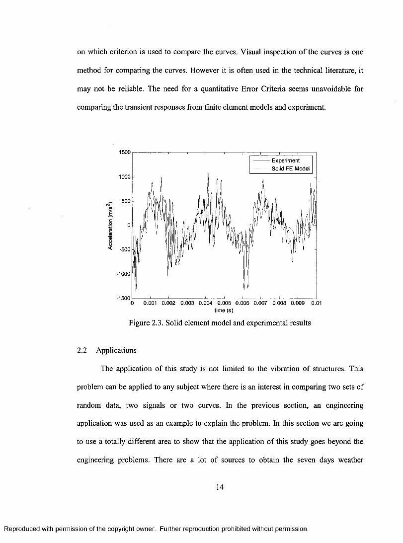
This graph shows the acceleration of a particular point in the structure caused by
an impact force or shock. The response presented in Figure 2.1 is only an experimental
result. Figure 2.2 shows the acceleration o f the same point obtained from a finite element
model with shell elements, and the experimental result. Figure 2.3, shows the acceleration
o f the same point from the experiment and a finite element model with solid elements.
The experimental results in both Figure 2.2 and Figure 2.3 are the same. The only
difference between these two plots is the results obtained from the two different finite
element models.
1500
1000
_ 500
II » 0)0)B< -500
-1000
-1500
Experiment Shell FE Model
J ___________ L_ _l____________L_
0 0.001 0.002 0.003 0.004 0.005 0.006 0.007 0.008 0.009 0.01time (s)
Figure 2.2. Shell element model and experimental results
The purpose of these graphs is to show the experimental verification o f the finite
element model. Which finite element analysis procedure provides a better match to the
experimental data? This is a complex question that may have different answers depending
13
Reproduced with permission of the copyright owner. Further reproduction prohibited without permission.
Page 29
on which criterion is used to compare the curves. Visual inspection o f the curves is one
method for comparing the curves. However it is often used in the technical literature, it
may not be reliable. The need for a quantitative Error Criteria seems unavoidable for
comparing the transient responses from finite element models and experiment.
1500— Experiment- - Solid FE Model
1000
500
t
! ■< -500
-1000
-15000 0.001 0.002 0.003 0.004 0.005 0.006 0.007 0.008 0.009 0.01
time (s)
Figure 2.3. Solid element model and experimental results
2.2 Applications
The application o f this study is not limited to the vibration o f structures. This
problem can be applied to any subject where there is an interest in comparing two sets of
random data, two signals or two curves. In the previous section, an engineering
application was used as an example to explain the problem. In this section we are going
to use a totally different area to show that the application o f this study goes beyond the
engineering problems. There are a lot o f sources to obtain the seven days weather
14
Reproduced with permission of the copyright owner. Further reproduction prohibited without permission.
Page 30
forecast, but which one is more accurate and reliable? Obviously the only way to
investigate the reliability o f these sources is looking at their previous records. To answer
this question we need to look at the seven days forecasted temperature and the measured
temperature after seven days. To treat each source with the fair condition, we compare
each source forecast with its own measured temperature after seven days. Figure 2.4 and
Figure 2.5 show the forecasted and recorded temperature from the Weather Channel and
Fox News in Las Vegas from Nov 15, 2005 to Dec 30, 2005 [25, 26].
2
ia>E(U
80
75
70
65
60
55
50
45
/ ' ------ Meas ured Tem p-------7 Day Forecast
l A M - A\ ^ / V - V
oO'
.r> S3 S3S3 03 O' -> -> S3 S3o O' o ô o O' o O'
o O o O' o C3 o OO' O' O'Date ^
O' O' O' oO'
Figure 2.4. Seven days forecast and recorded temperature from Fox News [25]
It is hard or maybe even impossible to recommend any o f these sources without
having a comparison criteria. This example shows the application o f error criteria is not
limited to the engineering applications and can be useftil in many other subjects.
15
Reproduced with permission of the copyright owner. Further reproduction prohibited without permission.
Page 31
80 Measured Temp 7 Day Forecast75
70
65
60
55
50
45
O' %oO'
%%
%%
%%
Date
o%
O'%
% %%
%%
Figure 2.5. Seven days forecast and recorded temperature from Weather Channel [26]
2.3 Error Criteria Objectives
A consistent error criterion for comparing two transient curves was not found in
the structural dynamic literature. Several different methods are used by most researchers.
The most common methods are reviewed in this chapter. Advantages and disadvantages
are discussed for each method and recommendations are made for the most suitable for
structural dynamics problem.
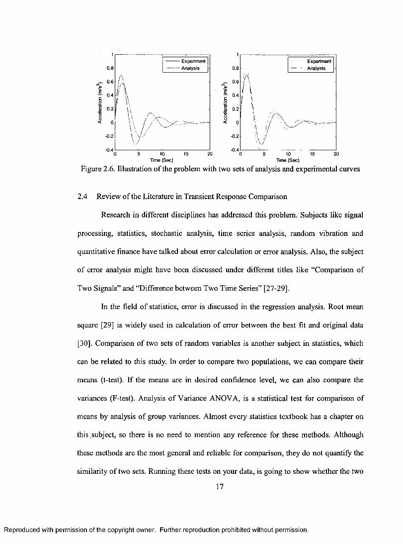
One might be interested to determine which set o f curves presented in Figure 2.6
is a better match. The word ‘set’ has been used because we are interested in comparing
two pairs o f curves. Generally there is one experiment and one analysis in each pair. The
objective is to determine which pair is more similar.
This illustration shows that the visual judgment is very subjective. If someone
says the set on the right plot in Figure 2.6 is closer to the experiment, unless he or she
does not bring a logical explanation the conclusion is not valid.
16
Reproduced with permission of the copyright owner. Further reproduction prohibited without permission.
Page 32
ExperimentAnalysis
ExperimentAnalysis0.8 0.6
_ 0.6 ^ 0.6
— 0.4 0.4
0.2 0.2
-0.2 - 0.2
-0.4 -0.420
Time (Sec) Time (Sec)
Figure 2.6. Illustration of the problem with two sets o f analysis and experimental curves
2.4 Review o f the Literature in Transient Response Comparison
Research in different disciplines has addressed this problem. Subjects like signal
processing, statistics, stochastic analysis, time series analysis, random vibration and
quantitative finance have talked about error calculation or error analysis. Also, the subject
o f error analysis might have been discussed under different titles like “Comparison o f
Two Signals” and “Difference between Two Time Series” [27-29].
In the field o f statistics, error is discussed in the regression analysis. Root mean
square [29] is widely used in calculation o f error between the best fit and original data
[30]. Comparison o f two sets o f random variables is another subject in statistics, which
can be related to this study. In order to compare two populations, we can compare their
means (t-test). If the means are in desired confidence level, we can also compare the
variances (F-test). Analysis o f Variance ANOVA, is a statistical test for comparison of
means by analysis o f group variances. Almost every statistics textbook has a chapter on
this , subject, so there is no need to mention any reference for these methods. Although
these methods are the most general and reliable for comparison, they do not quantify the
similarity o f two sets. Running these tests on your data, is going to show whether the two
17
Reproduced with permission of the copyright owner. Further reproduction prohibited without permission.
Page 33
sets o f data are close or not, but they are not able to determine how much these sets o f
data are close together.
The moment method is another way for comparison o f two sets o f data. This
method is also used by the scientists in the subject o f signal processing [28] and statistical
signal processing subjects [27]. In this method each signal or curve will be represented
with its moment, like raw moments or central moment [31]. Federal Highway
Administration (FHWA) [24] has a validation procedure for comparing two signals. The
main part o f this procedure uses method o f moments for validation o f models with tests
or experimental results. Smallwood [32] and Cap [33] use the band limited temporal
moments to calculate a normalized error between two transient time histories. With this
method, they calculate the normalized error over different bandwidths.
Geers [34] defines an error measure for the comparison o f calculated and
measured transient time histories. His suggested error factor assigns a single numerical
value to the discrepancy existing over a specified comparison period. Information
regarding the nature o f the discrepancy is provided by the magnitude and phase error
factors, which constitute orthogonal components o f error. Geer’s work had been followed
by Whang, Gilbert and Zilliacus [35]. They have introduced two correlation measures for
comparing calculated and measured response histories. The first one is an error index,
which is a simplification o f root sum square error factor. The second one is an inequality
index that is a simplification o f Theil’s Inequality.
IB
Reproduced with permission of the copyright owner. Further reproduction prohibited without permission.
Page 34
2.5 Error Calculation Methods
The error calculation methods can be divided to two different categories: the full
and the partial error calculation methods. The full methods calculate the error over the
whole curve such as root mean square, while the partial calculation methods consider
specific characteristic o f the curve as a criterion. In partial calculation method, the error is
defined as the error between the characteristics o f each curve. For example, one can pick
‘the maximum peak’ as a criterion. With this criterion, the error would be the difference
between the maximum peaks o f two sets o f data.
The full error calculation methods are regular (common) method, root mean
square (RMS), band limited temporal moment method and the method o f moments. The
partial error calculation methods are: ‘error in maximum value’ and ‘peak counting
methods’. O f course there are more error criteria than the methods discussed here, but
they have either no application in our problem or they do not quantify the error as a value
for comparison purposes.
2.5.1 Regular Method
This is the most common method used for error calculation. One value is used as
the reference when calculating the error with this method. For example the analytical
answer can be the reference if it is available. Error can be calculated as the difference
between two curves at each particular point (or time), divided by the reference value. The
following formula shows how to calculate the error between finite element model and
experiment.
X{t) — A(t)E(t) = -
%(f)
19
Reproduced with permission of the copyright owner. Further reproduction prohibited without permission.
Page 35
where X(t) is the acceleration measured by an accelerometer mounted on a
vibrating structure and A(t) is the acceleration o f the same point obtained from finite
element model. Since X(t) and A(t) are functions of time, the error is also time
dependent. For the sake o f comparison, we need a single value over a comparison time
period. The regular error method fails to do that. A suggestion to solve this problem is to
take the average values o f the error to get a single number.
The accelerations plotted in Figure 2.7 are from experimental and finite element
analysis o f a rectangular steel flat plate. Shell elements have been used to model the plate
for finite element analysis. The accelerometer has been placed 0.52 m from impact point.
An instrumented hammer has been used to excite the plate.
0.52(m) from impact1500
— Experiment Shell FE Model
1000
600
I ” 0)
I< -500
-1000
-15000.001 0.002 0.003 0.004 0.005 0.006 0.007 0.008 0.009 0.01
time (s)
Figure 2.7. Accelerations obtained from experimental results and shell finite elementmodel
20
Reproduced with permission of the copyright owner. Further reproduction prohibited without permission.
Page 36
Figure 2.8 shows the error signal ealculated with the regular method. The error at
each instant is the difference between two accelerations divided by the experimental
acceleration at that instant.
250
200
150
100
IUJ
-50
-1000.001 0.002 0.003 0.004 0.005 0.006 0.007 0.008 0.009 0.01
time (s)
Figure 2.8. Error calculated with the regular method
This method has two disadvantages that make it a less suitable method for the
application o f this study. In fact because o f these reasons, it is not useful for many
applications. The first problem is that every time the reference signal becomes zero, the
error is not defined. In the ease o f the flat plate presented in Figure 2.7, the experimental
signal is considered as the reference signal. Every time this signal has a value o f zero, the
value o f error is not defined. Most computer software including MS Excel and
MATLAB, substitute a very large number when a number is divided by zero (oo). That is
why there are big spikes in the error plotted in Figure 2.8. The actual number shown on
21
Reproduced with permission of the copyright owner. Further reproduction prohibited without permission.
Page 37
the plot is random because the plotting software substitutes a large number for oo. This
does not mean there is a large error on those instances. It simply means that the value o f
experimental signal is zero on those instances. The regular method does not quantify the
similarity o f the two curves (signals). This is the second disadvantage o f this method. It
means we do not obtain a single value for the error. This problem makes it impossible to
use this method for the comparison proposes.
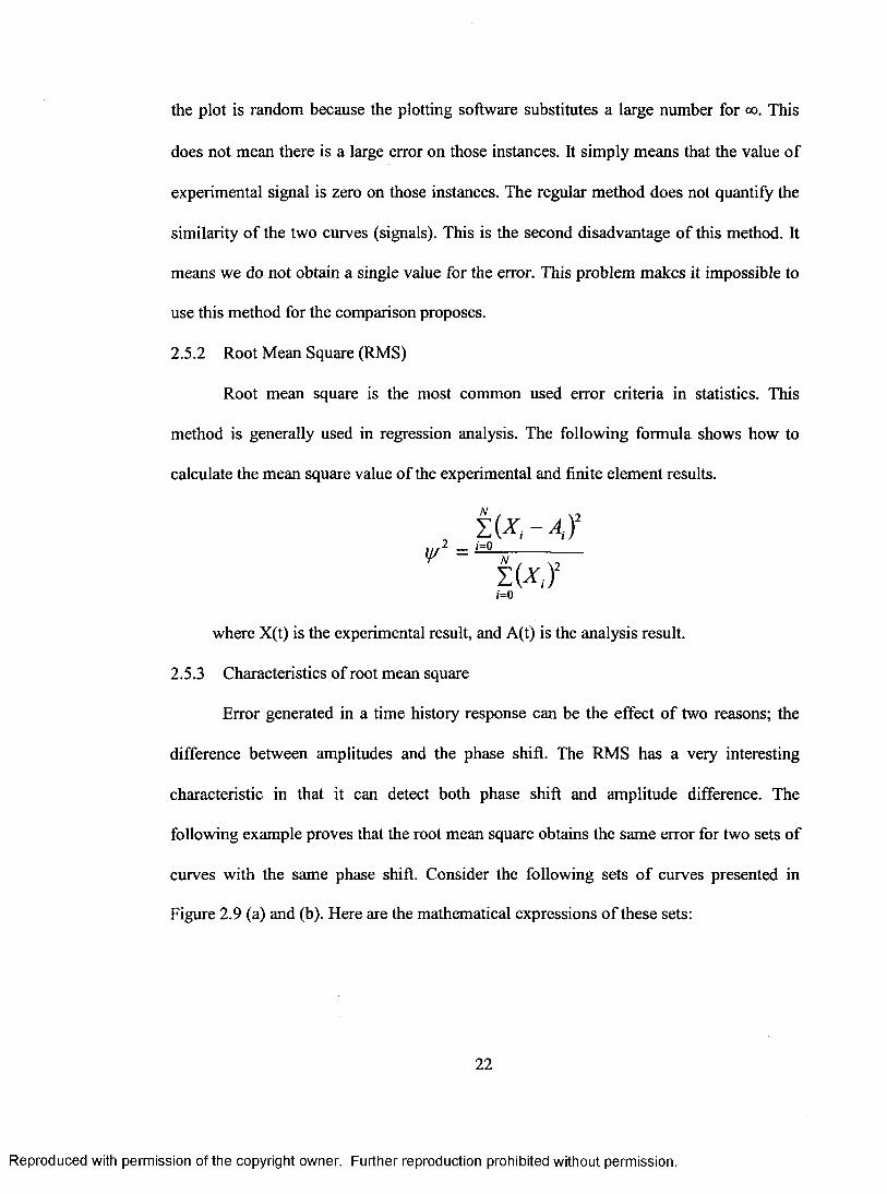
2.5.2 Root Mean Square (RMS)
Root mean square is the most common used error criteria in statistics. This
method is generally used in regression analysis. The following formula shows how to
calculate the mean square value o f the experimental and finite element results.
j= 0
where X(t) is the experimental result, and A(t) is the analysis result.
2.5.3 Characteristics o f root mean square
Error generated in a time history response can be the effect o f two reasons; the
difference between amplitudes and the phase shift. The RMS has a very interesting
characteristic in that it can detect both phase shift and amplitude difference. The
following example proves that the root mean square obtains the same error for two sets o f
curves with the same phase shift. Consider the following sets o f curves presented in
Figure 2.9 (a) and (b). Here are the mathematical expressions o f these sets:
22
Reproduced with permission of the copyright owner. Further reproduction prohibited without permission.
Page 38
15/ Set
y I = sin(/)
y 2 = s in ( / - —)
2nd Set
y 3 =sin(/ + y )
• 5;r.y 4 - sin(/ + — )
6
0.5
i?
4 6 8 10 120 2Time (sec)
0.5
Ii?
100 2 4 6 8 12Time (sec)
Figure 2.9. (a), (b). Two sets o f curves with the same amplitude and same phase shift
The mathematical representations o f first set o f curves show that there is no
difference in amplitudes, but they have a 90“ phase shift. The curves presented in the
second set have the same phase shift with no change in amplitudes. This means that these
two sets o f curves are exactly similar to each other. In other words one cannot say that yi
and Y2 are more similar compare to yj and y4 or vice versa. Generally speaking the error
between yi and y; is equal to the error between ya and y4 . See if we can confirm this by
calculating the root mean square (\j/). Here is calculated root mean square for each set of
curves.
V (yi, yz)= 1.41
w (Y3, y4)= 1.41
(Corresponding to Fig. 9(a))
(Corresponding to Fig. 9(h))
23
Reproduced with permission of the copyright owner. Further reproduction prohibited without permission.
Page 39
With a similar example, it can be shown that one can obtain an almost equal RMS
for signals with the same difference in amplitudes. The only disadvantage o f this method
is that there is only one value for the error. This means if there is both phase shift and
amplitude difference in two signals, the RMS will show the difference, but it is
impossible to determine which one o f these sources contributes more in generating the
error.
2.5.4 Moment Method
In order to compare two curves, we can compare the relative absolute difference
o f characteristic values. Each set o f data can be characterized by a few numbers that are
related to its moments. The moments o f a random variable are the expected values o f its
powers [31]. It is assumed that if the difference between two signals in terms o f a
particular order is less than 2 0 percent, the signals are considered to be sufficiently close
to one another [24]. It is useful to review the definitions and formulas o f different
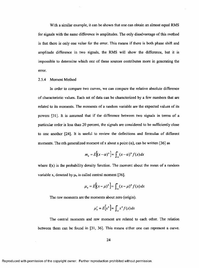
moments. The nth generalized moment o f x about a point (a), can be written [36] as
= £ [ ( x - a ) " ] = £ ( x - « ) " / W ^
where f(x) is the probability density function. The moment about the mean o f a random
variable x, denoted by pn is called central moment [36].
- / / )" ]= [ j , x - / x Y f { x ) d K
The raw moments are the moments about zero (origin).
= ^ [^ " ]= [ ^ x " f { x )d x
The central moments and raw moment are related to each other. The relation
between them can be found in [31, 36]. This means either one can represent a curve.
24
Reproduced with permission of the copyright owner. Further reproduction prohibited without permission.
Page 40
Instead of presenting a curve with its consequence moments, we can present it with the
meaningful quantities (like mean, variance,...) derived from its moments.
The mean
The first raw moment is called mean (p).
M = H[ = ^[x]= £ x /(x )d x
For discrete uniform distribution, f(x)= Pr[x=k]= 1/N, where N is the number o f
collected data. In this ease, the mean is simply the average o f these data values.
Therefore, it is the sum of the data values divided by N [37].
_ sum of data valuesX -------------------------------------
N N
The symbol Z represents the sum of data values.
The Variance
The second central moment is called variance (a^).
^ 2 = e \ ^ x - ^ Y \ = ^ ^ { x - f{ x )d x
For a discrete uniform distribution with N data values, the sample variance can be
defined as [37]:
The variance some times is denoted by var(X) or V(X). The square root of
variance is called standard deviation and it is denoted by (o).
Skewness
The third central moment is called skewness.
=eYx-mŸ\= mŸ f{x)dx
25
Reproduced with permission of the copyright owner. Further reproduction prohibited without permission.
Page 41
Skewness is the symmetry o f a distribution about its mean. Figure 2.10 shows two
distributions with positive and negative skewness [38].
f(x)f(x)
»XX XX
Positive Skewness Negative Skewness
Figure 2.10. Example o f curves with positive and negative skewness
If the curve, at the left side o f the mean line, is more stretched compare to the
right side, then it has positive skewness. If the reverse is true, it has negative skewness
(Figure 2.10). If the curve is equally stretched on both sides on the mean line, it has zero
skewness. For example, the normal distribution has zero skewness. Some literature use
normalized skewness instead o f the skewness. The normalized skewness o f a distribution
is defined to be
/ 3
Kurtosis
The fourth central moment is called kurtosis.
/ / 4 = F :[(x - /i) '']= f { x ) d x
Kurtosis is the peakedness o f a distribution. The normalized kurtosis is defined as
26
Reproduced with permission of the copyright owner. Further reproduction prohibited without permission.
Page 42
/^4 -/ 4
For a normal distribution, kurtosis is equal to 3. Figure 2.11 shows a curve and
plotted with its normal distribution in the same graph. If the value o f kurtosis is more
than 3, there would be presence o f peaks o f high value. In this case the peak o f the
probability density function is higher than its normal distribution. The curves with
kurtosis less then 3 have a flat probability density function, and they have a smaller peak
compare to their normal distribution [38].
f(x)
p > 3
NormalDistribution
| i < 3NormalDistribution
->X X
Figure 2.11. Example o f curves with kurtosis greater and less than 3
The moment method defines a curve with four quantities. In order to compare two
curves, we can compare the moments o f each curve, with the other one, i.e. 1 st moment
with 1st moment, 2"* moment with 2"* moment and so on. Having more than one quantity
for comparison makes it easier to understand the source o f error. The moment method
shows whether the error is coming from amplitude difference or phase shift. On the other
hand, having a couple o f quantities as error instead o f one value, some times would be
confusing. For example assume that signals Yi and Y] show small error in 1®* and 2"'*
27
Reproduced with permission of the copyright owner. Further reproduction prohibited without permission.
Page 43
moments but large error in 3" and 4*'’ moments. Vice versa, signals Y 3 and Y4 show large
error in 1®* and 2"* moments but high error in large error in 3' '* and 4*'’ moments. In this
case or cases similar to this example, there would not be a solid result o f the similarity
between two sets o f signals, and it is dependent to the user’s interpretation. In order to
compare two signals with the moment method, they must be stationary. It means that all
o f their statistical properties should not vary with time. Because o f this property the
application o f moment method is very limited.
2.5.5 Method o f Temporal Moments
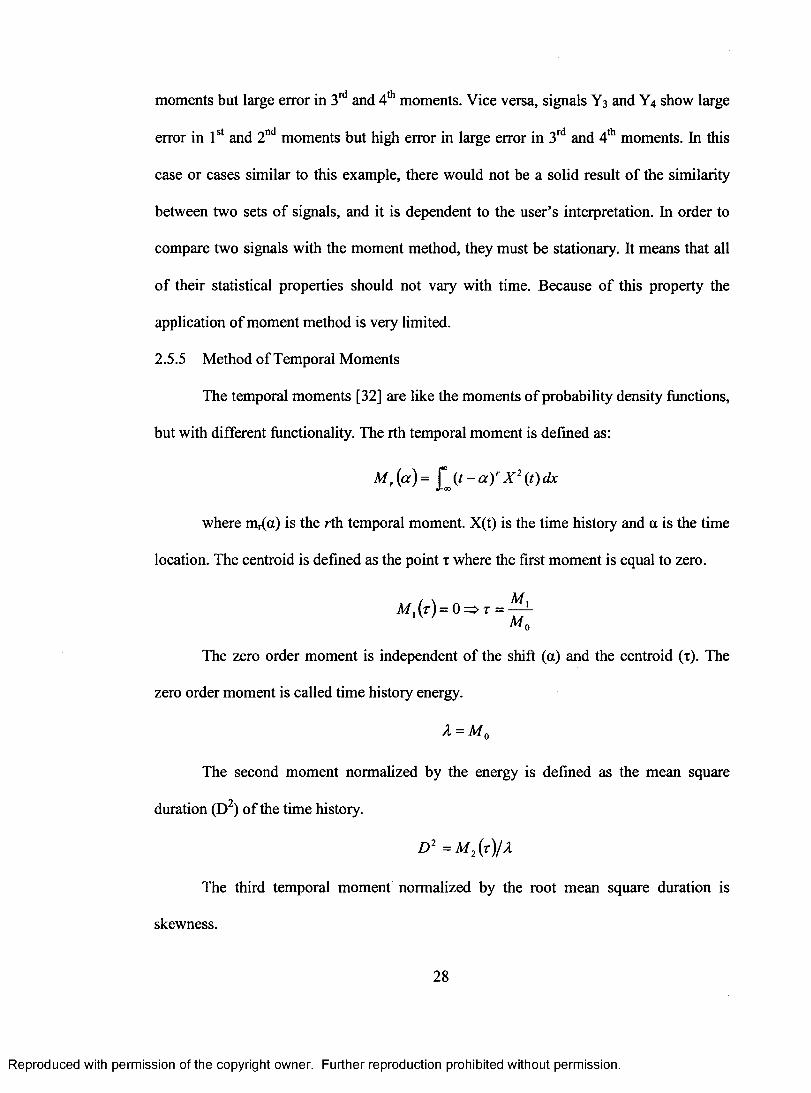
The temporal moments [32] are like the moments o f probability density functions,
but with different functionality. The rth temporal moment is defined as:
M ,(ar)= [ y - a y X \ t ) d x
where m ^a) is the rth temporal moment. X(t) is the time history and a is the time
location. The centroid is defined as the point x where the first moment is equal to zero.
Mj (t )= 0=> T =Mo
The zero order moment is independent o f the shift (a) and the centroid (x). The
zero order moment is called time history energy.
A = Mo
The second moment normalized by the energy is defined as the mean square
duration (D^) o f the time history.
= m X x)IX
The third temporal moment normalized by the root mean square duration is
skewness.
28
Reproduced with permission of the copyright owner. Further reproduction prohibited without permission.
Page 44
S = S J D
The skewness presents the shape o f the function, as it was described on the
moment method. A positive skewness indicates high amplitudes on the left o f the
centroid, and a long low amplitude tail on the right o f the centroid.
The forth normalized central moment is called kurtosis. The kurtosis is useful for
time histories that have more than one maximum.
K = K J D
The objective is to characterize each time history with as few as parameters as
possible. The first few parameters are the centroid (x), the time history energy (E), the
root mean square duration (D), the normalized skewness (S), the normalized Kurtosis
(K). Each time history can be represented with these parameters (x, X, D, S, K). In order
to compare two time histories, we can compare the characteristics o f them. The method
of temporal moments only characterizes the transient time histories, so it is not applicable
for the cases that part o f transient response is in the interest o f the researchers. Also, this
method is not applicable for the time histories that cannot be divided to transient and
steady state response like the weather forecast example.
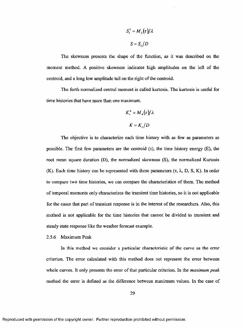
2.5.6 Maximum Peak
In this method we eonsider a partieular eharacteristic o f the curve as the error
criterion. The error calculated with this method does not represent the error between
whole curves. It only presents the error o f that particular criterion. In the maximum peak
method the error is defined as the difference between maximum values. In the case o f
29
Reproduced with permission of the copyright owner. Further reproduction prohibited without permission.
Page 45
existing both positive and negative values, the absolute values must be considered for
error calculation.
Max^X (t)|) - Mox(|^(t)|)Peak ■xlOO
Max(\X{t)\)
To illustrate this method lets present the experimental and analysis results o f the
quarter inch steel plate under the effects o f an impact for 0.004 s (Figure 2.12).
1400Maxiimun Peak of Expeiiinent Experiment
Solid Model1200
Rla.xiimun Peak of Analysis
1000
& 800
600
400
200
2.5 3.50.5time (s) •3X 10'
Figure 2.12. Illustration o f maximum peak error calculation method
The absolute maximum experimental and analysis accelerations are 1361.6 and
1136.1 m/s^ respectively.
Peak Error; g ^ . ^61.6-1136.1 ^1361.6
30
Reproduced with permission of the copyright owner. Further reproduction prohibited without permission.
Page 46
This method will be applicable in particular cases where only the maximum
acceleration is important. This method is time independent. In other words, to use this
method, the time at which maximum acceleration happens, should not be important.
Having a small error between the maximum value o f two curves or signal does not mean
that those two curves or signals are similar, unless it is justified properly. Even if it is
justified by the author, it is not expandable to other cases and it is valid only for that
particular case.
2.5.7 Peak Counting Methods
This method is another way to approach the comparison problem with considering
partial characteristics o f a curve or signal. The criterion used in this method is the number
o f times a signal exceeds a certain value. This method was originally developed for the
study o f fatigue damage in structures [38], but with a little modification it can be used for
the comparison o f two signals.
The objective is to count the peaks above or below a certain value. This value can
be any number, like the mean o f amplitudes or any other predefined value. If both signals
have the same number o f peaks above that value, they are said to be similar to each other.
This is the simplest way to apply the peak counting method. Depending on the accuracy
o f the similarity o f two signals, one can use other peak counting methods such as Range-
restricted peak count or Level-restricted peak count [38] for the purpose o f comparison.
Let’s re-demonstrate the experimental and analysis results o f the quarter inch steel
plate under the effects o f an impact for 0.004 seconds (Figure 2.13). With this method,
we would like to compare the two accelerations with number o f times they exceed 1 0 0 0
m/s^.
31
Reproduced with permission of the copyright owner. Further reproduction prohibited without permission.
Page 47
1400
2 peaks counted from experiment1200
] peak counted from analysis
1000
& 800
600
400
200
0.5 2.5 3.5time (s) ■3
X 10
Figure 2.13. Comparison o f two accelerations with peak counting method
The experimental result shows that the acceleration o f the structure twice exceeds
1000 m/s^. The finite element analysis shows only one peak higher than 1000 m/s^. In
this case there would be a 50% error between experimental and analysis result.
2 . 6 Summary o f Error Calculation Methods
This study searches for a quantified comparison factor to compare two sets o f
data, curves or signals. The error generated between two curves can be the effect o f phase
shift or amplitude difference or both. The error calculation methods can be divided to
either the full or partial methods. The full methods calculate the error over the whole
curve such as root mean square, while the partial calculation methods consider specific
characteristic o f the curve as a criterion. Regular Method, Root Mean Square (RMS),
32
Reproduced with permission of the copyright owner. Further reproduction prohibited without permission.
Page 48
Moment Method, Method o f Temporal Moments, Maximum Peak and Peak Counting
Methods are the methods presented in this study.
Regular method is easy to use, but the error calculated with this method is time
dependent. For the sake o f comparison o f two signals, we need a single value over a
comparison time period. This makes the regular method not applicable for the objective
o f this study. The moment method determines whether the error is coming from
amplitude difference or phase shift, but in order to compare two signals with the moment
method they must be stationary. This property o f moment method makes it limited for
most applications, and not useful for comparison purposes. The method o f temporal
moment characterizes the transient time histories, so it is not applicable for the cases that
part o f transient time history is in the interest o f the researchers. This method is not
applicable for the time histories that caruiot be divided to transient and steady state
response.
Both maximum peak method and peak counting method consider a particular
characteristic o f a curve as error criterion. In many cases, the peak amplitude is the result
that is o f most interest; therefore it makes sense to use this criterion to compare two
signals.
Root mean square can detect both phase shift and amplitude difference. Since
only one value for error can be obtain from this method, it is impossible to determine the
source o f the error. Having said that, having a single value as the error quantity makes it
easy to compare two sets o f curves.
33
Reproduced with permission of the copyright owner. Further reproduction prohibited without permission.
Page 49
All o f these methods have advantages and disadvantages. Unfortunately, there is
not a single criterion that seems to be the best for comparing transient acceleration curves
due to impact loading.
2.7 The Dissimilarity Factor (DF)
The Dissimilarity Factor (DF) is defined to have a single value for comparison o f
two sets o f curves. The dissimilarity factor is a linear combination o f some o f the error’s
defined in pervious sections. The general form o f the dissimilarity factor as follows:
DF W2 E 2 + w E + w^E^
where Ei ... E4 are the values o f error and w, ... W4 are the weights assigned to each
error. The summation o f all weight factors must be one, i.e. Wi+W2 +W3 +W4 = l. The
maximum peak value, zeroth, first and second moment method are the four error method
contributing to the calculation o f dissimilarity factor. The maximum peak value, zeroth
and first moment method detect the amplitude difference. In the application o f this study,
the difference between amplitudes is more important, so the weight factor assigned to
these errors is twice as the weight factor assigned to the second moment method. So, the
final form o f the dissimilarity factor can be written as follows:
where Ei is the maximum peak value, E2 is the zeroth moment, E 3 is the first moment and
E4 is second moment.
34
Reproduced with permission of the copyright owner. Further reproduction prohibited without permission.
Page 50
CHAPTER 3
EXPERIMENTAL CALIBRATION OF FINITE ELEMENT ANALYSIS
3.1 Introduction
This chapter investigates the dynamic response o f a simple structure used for
impact testing. Performing the experiment on a simple structure is the most important
part o f any type o f experimental verification projects. The first step o f every experimental
project is to determine whether the method of approach is able to solve a simple problem
or not. This ehapter demonstrates the procedure and setup for experimental verification of
the Finite Element Analysis (FEA) o f a simple structure. A solid bar or beam is one o f the
simplest structures that can be employed for the testing o f dynamic behavior o f the
structures. Modal analysis is the first step in investigation o f dynamic response of
structures. Once the modal analysis o f the system is verified experimentally, we can look
at the time history response o f a shock or impact to the system. The impulse hammers are
used to excite a system with a known input force so the dynamic response o f the system
can be analyzed.
3.2 Geometry o f the Bar
Figure 3.1 shows the dimensions o f the solid cylinder with the base diameter o f
0.0381 m and height o f 0.1968 m. The mass o f the cylinder is 1.711 kg.
35
Reproduced with permission of the copyright owner. Further reproduction prohibited without permission.
Page 51
Figure 3.1. Dimensions o f the Bar
The eylinder has been made o f steel. The material properties o f the steel will be
mentioned in the modeling analysis part.
3.3 Experimental Procedure
The experimental procedure is the same throughout the rest o f the dissertation.
The only difference between experiments throughout this project is the structure, which is
the subject o f the experiment. First the equipment used in this project has been described,
and then test setup and experimental procedure is explained. The last part o f this section
talks about experimental results obtained from the solid uniform bar.
3.3.1 Equipment
An accelerometer and impact hammers with hard tips are used to make the
necessary measurements for the test. The impact hammers used in the experiments can be
seen in Figure 3.2 - 3.4. Figure 3.5 shows the accelerometer used in the experiment. The
pertinent information for the impact hammers and the accelerometer can be found in
Tables 3.1 -3.3.
36
Reproduced with permission of the copyright owner. Further reproduction prohibited without permission.
Page 52
Figure 3.2. PCB 086C02 impulse hammer (Small)
Figure 3.3. PCB 086C20 impulse hammer (Large)
37
Reproduced with permission of the copyright owner. Further reproduction prohibited without permission.
Page 53
Figure 3.4. Comparison o f Large and small impulse hammers
w
Figure 3.5. PCB 352C22 ceramic shear ICP accelerometer
38
Reproduced with permission of the copyright owner. Further reproduction prohibited without permission.
Page 54
Table 3-1. PCB 086C02 Modally Tuned Impulse Hammer [39]
Model No. 086C02Perform ance Units (SI)Sensitivity (± 15%) I1.2m V /NMeasurement ± 440 N pkFrequency Range (Hard Tip) 8 kHz
(Medium Tip) 2.5 kHzResonant Frequency > 2 2 kHzPhysicalSensing Element QuartzHammer Mass 0.16 kgExtender Mass Weight 75 gmHead Diameter 1.57 cmTip Diameter 0.63 cmHammer Length 2 1 . 6 cm
Table 3-2. PCB 086C20 Modally Tuned Impulse Hammer [39]
M odel No. 086C20Perform ance Units (SI)Sensitivity (± 15%) 0.23 mV/NMeasurement ± 22,000 N p kFrequency Range (Hard Tip) 1 kHzResonant Frequency > 12 kHzPhysicalSensing Element QuartzHammer Mass 1 . 1 kgHead Diameter 5.1 cmTip Diameter 5.1 cmHammer Length 37 cm
39
Reproduced with permission of the copyright owner. Further reproduction prohibited without permission.
Page 55
Table 3-3. Accelerometer information [39]
M odel No. 352C22Perform ance Units (SI)Sensitivity (± 15%) 1.0mV/(m/s^)Measurement ± 4900 m/s^ pkFrequency Range (± 5%) I.O to 10,000 Hz
(± 1 0 %) 0.7 to 13,000 HzResonant Frequency > 5 0 kHzPhysicalSensing Element CeramicSensing Geometry ShearSize 3.6 mm x 11.4 mm x6.4 mmWeight 0.5 gmMounting Adhesive
The accelerometer calibrator listed in Table 3.4 is used to calibrate the
accelerometers. The accelerometer is attached to the calibrator using a threaded adapter.
This calibration is performed using PCB 394C06 hand held calibrator (Figure 3.6)
connected to Pulse hardware. In order to have more precise experiments, the
accelerometers have been calibrated before each set o f experiments.
Figure 3.6. PCB 394C06 hand held calibrator
40
Reproduced with permission of the copyright owner. Further reproduction prohibited without permission.
Page 56
Table 3-4. Accelerometer Calibrator information [39]
M odel No. 394C06Perform ance Units (SI)Operating Frequency (± 1%) 159.2 HzAcceleration Output (± 3%) 9.81m/s"^ rmsMaximum Load 2 1 0 gmPhysicalSize (Diameter) 56 mmWeight (with batteries) 900 gm
In order to process the signals generated by the hammer and the accelerometer we
need to connect them to a computer. This is accomplished by using a Pulse Data
Acquisition (DAQ) Hardware made by Briiel & Kjær [40] (Figure 3.7). The Pulse
Hardware accompanied by the Pulse software installed on a Laptop is a portable data
processing system suitable for vibration testing.
Figure 3.7. A six FFT input channel Pulse data acquisition hardware
The Pulse software is used for analyzing the data. Fast Fourier Transform
Analyzer (FFT) in Pulse software is used to perform modal analysis on structures. Time
41
Reproduced with permission of the copyright owner. Further reproduction prohibited without permission.
Page 57
Capture Analyzer is another package in Pulse software, which enables us to obtain the
time history response o f structures to shock and impacts.
Table 3-5. Pulse data acquisition hardware information [40]
M odel No. Portable PULSE - 3560CDynamic Range (FFT) 160 dBReal-time Rate 25.6 kHzI/O (FFT & Time Capture) 6 channels
3.3.2 Test Setup and Procedure
The whole test setup includes an A-fi-ame structure to support a hanging mass, a
known cylindrical mass, accelerometer, impulse hammer. Pulse Hardware and a laptop
computer with Pulse software (Figure 3.8). The A-frame supports one o f the masses by a
cable and an accelerometer is then mounted to one end of the mass. The accelerometer is
attached to the data acquisition hardware, which provides power for internal circuitry and
links the accelerometer to the computer. The impulse hammer is connected to the
computer in the same manner as the accelerometer. Performing the experiment requires
connecting the accelerometer and hammer to the Pulse hardware, and then connect the
hardware units to the computer. There is a routine setup procedure for Pulse Lab
Software. This includes setting up FFT and Time analyzer. Next, we impact the hanging
mass with the impact hammer. A drop of super glue has been applied to stick
accelerometer on the cylinder body. After mounting each accelerometer on the cylinder,
the cylinder has been hit by the hammer three times, and three different data has been
collected to insure the repeatability o f the experiment for each accelerometer. Mounting
42
Reproduced with permission of the copyright owner. Further reproduction prohibited without permission.
Page 58
accelerometer on structures with super glue is a reliable technique for impact testing up to
10,000 Hz frequency range [39].
Figure 3.8. A-frame and pendulum setup
3.3.3 Experimental Results
The experimental results include two parts: Modal analysis and Time history
response. Fast Fourier Transform (FFT) analyzer is used for the modal analysis o f the
structure. Time capture analyzer is used for time response o f the structure. The
measurement units for the accelerometer and hammers are m/s^ and N respectively.
3.3.3.1 Modal Analysis
The peaks on FFT analyzer show the natural frequency o f the structure. Figure 3.9
shows the FFT plot o f the round bar. The peak corresponding to the 8'^ mode is not very
43
Reproduced with permission of the copyright owner. Further reproduction prohibited without permission.
Page 59
obvious. This peak belongs to the torsional natural frequency. It is very hard to excite this
mode with impact to the solid bar. Table 3-6 presents the natural frequencies o f the solid
bar.
i n n n n - ,
i n n n1 u u u
o"Û i n n 12 lu u
c10g 1U
i 11
O 1U. 1 i
C) 3000 6000 9000 Frequency (Hz)
12000 15000
Figure 3.9. Experimental FFT plot o f the round bar
Table 3-6. Experimental natural frequencies o f the round bar
ModeExperimental Natural
Frequency (KHz)
7 4.38 8.49 10.410 13.4
3.3.3.2 Time History
The acceleration and force in the time domain should have a sharp peak at the
maximum impact force and quickly damp out to zero Figure 3.10 and Figure 3.11. If the
signal has multiple peaks the test can be disregarded. The frequency range o f the load cell
44
Reproduced with permission of the copyright owner. Further reproduction prohibited without permission.
Page 60
within the impulse hammer is 2500 (Hz). This force will be used for finite element
analysis later on in this chapter, so the force data has been filtered at 2500 Hz (Figure
3.10 and Figure 3.11). The time history response has been filtered at 10,000 Hz because
the accelerometer frequency range is 1.0 to 10,0000 Hz. The sampling rate for data
presented in Figure 3.10 and Figure 3.11 rate is 65536 Hz.
500
400
300
zg 200 £
100
1000.001 0.002
Time (s)0.003 0.004
Figure 3.10. Applied force measured by small impulse hammer to the round bar
3.3.3.3 Coherence
Coherence measures the similarity o f vibration in two loeations. The two
locations for the hammer calibration are the force transducer on the hammer and the
accelerometer on the opposite side o f the impact surface on the mass. If the signals are
correlated the coherence function will be one (Figure 3.12). However, if the signals do
45
Reproduced with permission of the copyright owner. Further reproduction prohibited without permission.
Page 61
not have a coherence o f one the test is discarded and retested. If the coherence function is
not one, possible problems could be power supplies turned on, a glancing blow with the
hammer, bad wire connections, or low batteries in the power supplies. These should all
be checked before continuing the tests.
300
250
200
(N& 150Co
2■2 100 o<
-500.5 3.52.5
Time (s) •3X 10
Figure 3.11. Experimentally measured acceleration o f the round bar in the time domain
1000 1500f(Hz)
Figure 3.12. Coherence plot
2500
46
Reproduced with permission of the copyright owner. Further reproduction prohibited without permission.
Page 62
3.4 Natural Modes o f Vibration
It is possible to treat certain systems more rigorously, without discretization o f the
analytical model. In this section we will analyze beams in which mass and deformation
properties are continuously distributed. The best examples o f these structures are bars,
shafts and beams.
3.4.1 Longitudinal Vibration o f a Bar or Rod
The differential equation for longitudinal motion o f a thin rod can be written as
follows [41]:
£A(x )du{x,i)
dx= m{x)
d^u{x,t)dt^ (1)
which must be satisfied over the domain 0<x<L. In addition, u must be such that at the
end point for a ft-ee-ftee beam we have
^du{x,t)EA{x )-
dx(2)
x=0,L
In this chapter u(x,t) denotes the longitudinal displacement and y(x,t) is a
transverse displacement. Let us pursue further the case o f fi-ee-ffee rod, for which the
eigenvalue problem reduces to differential equation.
ddx
EA{x )dU {x)
dx= 03 m (3)
The homogenous boundary condition
EA{x )dU{x)
dx= 0 (4)
x=0,L
must be satisfied at the end point. For a uniform rod the eigenvalue problem reduces to
the solution o f the following differential equation.
47
Reproduced with permission of the copyright owner. Further reproduction prohibited without permission.
Page 63
^ ^ + / ) ’t /W = 0, (5)dx EA
The frequency equation can be obtained by applying the boundary conditions (Eq. 4) to
the longitudinal vibration differential equation (Eq. 5).
sin = 0 (6)
Calculation o f natural frequencies
sin P^L = Q => P^L = rn Where r=0,1,2,...
considering m is mass per unit length, m = ^ = = pA
3.4.2 Torsional Vibration o f a Shaft or Rod
If 6(x,t) represent the angle o f twist o f a cross section at the point x and at time t, the
equation o f motion in torsion is [41]
dx+ m^(x,t)=l{xŸ (9)
dx
G is the shear modulus and J(x) is a geometric property of the cross section, which in the
case o f a circular cross section is polar moment o f inertia.
(ft))32
48
Reproduced with permission of the copyright owner. Further reproduction prohibited without permission.
Page 64
The product GJ(x) is called Torsional stiflfhess. I(x) is the mass polar moment o f
inertia per unit length o f bar and mj{x,t) is the external twisting moment per unit length o f
bar. In the case o f free vibration, rm(x,t)=0, and eq. 9 reduces to
Ôdx
G j{x)dO{x,t)
dx= l{x)
d % x ,t )d r (11)
The boundary conditions for a beam free at both ends are
^dO{x,t)GJ{x)-dx
= 0 ( 12)
Letting 6(x,t)=0(x)f(t) and recalling f(t) is harmonic, the eigenvalue problem reduces to
the differential equation
dx
and the boundary conditions are
G j{x)d@{x,i)
dx
G j{x)d@{x)
dx0
jc=0,Z.
at the ends.
Let the bar be uniform and denote
co^IGJ
so that eq. (13) reduces to
dx
Appling boundary conditions to eq. 16 give us the frequency equation.
sin P^L = 0
So that the natural frequencies are
(13)
(14)
(15)
(16)
(17)
49
Reproduced with permission of the copyright owner. Further reproduction prohibited without permission.
Page 65
sin P^L = 0 => P^L - rn Where r=0,l,2,.
(18)
for a cylindrical bar (rod), d J =nd^32
/ = - - 2 Z V p
(19)
3.4.3 Flexural Vibration o f Bars or Beams
In this section the transverse vibration o f beams is studied. Timoshenko [42] has
derived the general equation for transverse free vibrations o f beam as follows:
EI{x )^~Y dx = -p A d x ^ -YdP
(20)
Equation 20 will reduce to the following equation for the solid bar [41], [42]:
E l(x ) (x)y(x) (21)
In the above equation, Y(x) satisfies all four boundary conditions, two at each end. At a
free end the bending moment and the shearing force both vanish, and we obtain
= 0x=0,L
dxEl{x) d^yjx)
dk"= 0
(22)
(23)
In the particular case o f a uniform beam, where the flexural rigidity E l does not vary with
X, equation 21 will become
50
Reproduced with permission of the copyright owner. Further reproduction prohibited without permission.
Page 66
or
E I ^ ^ = o)^m y(x) ax
r p ^ - P * Y ( x ) = 0ax
(24)
(25)
where
P ^ — o x P =0,
At the free end, in the case o f uniform bar, the boundary conditions are
(26)
El{x)-(bP
= 0X = OyL
dxd^yjx)
dx^= 0
(27)
(28)x=0,L
All boundary conditions are natural. Consequently, by applying the boundary conditions
into eq. 25, we obtain the frequency equation.
cos(y0^z)cosh(y0,.z)= 1 (29)
This equation can be solved numerically for the eigenvalues Pr- The first few roots o f eq.
29 are
P,L=0,4.7, 7.9, 11.0, 14.1
The PrL=0 is for the rigid body modes. The natural frequencies are
PrL = a^=> i p . l f = ^
(30)
(31)
51
Reproduced with permission of the copyright owner. Further reproduction prohibited without permission.
Page 67
r V A A T . M .In the case o f solid rod, / = ----- = ----------- = A — and m = — = pA64 4 16 16 L
( i x ) e i p(32)
where ar = 0, 22.4, 61.7, 120.9, 199.9.
3.4.4 Results
We obtain the following equations for longitudinal, torsional and flexural
vibration o f a rod, in the last three previous sections.
2 L \ p
/ = - -2 L i p
f r =(8;r)L' V P
The diameter o f the bar is 0.0508 m and the length o f it is 0.1087 m. The bar is
made o f steel with modulus o f elasticity 207 GPa, shear modulus o f 81 GPa and its
density is 7850 kg/m^. The following table shows the natural frequencies o f the round bar
obtained analytically.
Table 3-7. Analytical natural frequencies o f the round bar
Mode Nat. Freq (KHz) Modal Characteristic
7 4.5 1®‘ Transverse Mode8 8.2 Torsional9 12.4 2"“ Transverse Mode10 13.0 Longitudinal
52
Reproduced with permission of the copyright owner. Further reproduction prohibited without permission.
Page 68
Note that the first six modes are rigid body modes and their corresponding natural
frequency is equal to zero.
3.5 Finite Element Analysis o f a Simple Structme
The last part o f this chapter is finite element analysis o f the simple structure. A
rigid round bar has been chosen as a sample for this purpose. The geometry o f the solid
cylinder is described in the beginning o f this chapter. The finite element analysis consists
o f two parts: Modal analysis and time history response. The modeling has been done in
the HyperMesh® and after applying the force, the model has been exported to LS-DYNA
for solution. The result has been filtered in the LS-DYNA post processor at 10000 Hz
corresponding to the experimental data.
3.5.1 Units
Units in LS-DYNA must be consistent. Table 3-8 shows a set o f units employed in
the modeling o f the structure. These units are base on the SI unit system. There are two
reasons for using SI units for the finite element modeling. The first reason is that implicit
method in LS-DYNA Version 9.60 for modal analysis does not give the right result if
geometry has been drawn in any other units except meters. We faced the same problem if
we used millimeters or inches as the length units in modal analysis in Altair OptiStruct®
version 7.0. The second reason is that Pulse, the experimental data analysis software,
works with SI units. The units o f results obtained and saved from this software are as
shown in Table 3-8, and that is the set o f units has been used in finite element analysis.
53
Reproduced with permission of the copyright owner. Further reproduction prohibited without permission.
Page 69
Table 3-8. Units used in he Modeling AnalysisUnits
Length meterTime secondMass kilogramForce newton
3.5.2 Material Properties
The round bar is made from cold rolled steel. Table 3-9 shows the material properties
o f the round bar [43].
Table 3-9. Material properties o f cold roll steel
Properties UnitsDensity P 7850 (Kg/m")Modulus o f elasticity E 207 (GPa)Poisson’s ratio V 0.3Yield stress o y 200 (MPa)
A plastic kinematic constitutive model, type 3 material card in LS-DYNA [44],
has been used to define the material for the structure. The following lines show the
material properties from LS-DYNA input file (.k file).
*MAT_PLASTIC_KINEMATIC$+++>++++1 -|-t-(-t->-H-H-2++++>+-H-+3++++>++++4++++>++++5++++>++++6++-H->++-H-7-l-H-l->+
MID RO E PR SIGY1 7850.0 207.0 E09 0.3 200 E06
3.5.3 Boundary Conditions
No geometric boundary conditions were applied to the model. In the experiment,
the cylinder hanged such a way that it can move freely in any direction. In the finite
element model it has been assumed that there is no constraint applied to the model, i.e.
free-free boundary conditions.
54
Reproduced with permission of the copyright owner. Further reproduction prohibited without permission.
Page 70
3.5.4 Applied Force
An impact force with a peak o f 440 N in less than 0.0006 s has been applied to the
model. The data for the force curve, shown in Figure 3.13, has been obtained from the
experiment captured by Pulse Software. The experiment procediu'e is explained in the
experiment section. For sake o f simplicity, this force considered as nodal force and has
been applied to the center node on the top plane of hat section (Figure 3.14).
450
400
350
300
250
S 200u_
150
100
-500.5 3.52.5
Time (s) ■3X 10
Figure 3.13. Force curve applied to the finite element models
The following lines show the nodal force implementation from LS-DYNA input
file (.k file).
*LOAD_NODE_SET$-t--H->f-t-+-t-H-+-H->+-H-t-2+-H-+>++++3+4-H->+-H-+4-H-H->-H-H-5++++>++++6+4-H->++++7++-H->4-
nsid dof Icid sf cid m l m21 2 3 -1.0
*SET_NODE_LIST 1
55
Reproduced with permission of the copyright owner. Further reproduction prohibited without permission.
Page 71
7756^DEFINE CURVE 30.0000000000, 0.00000
0.0019531250, 0.00000
Figure 3.14 shows the impact point and the accelerometer location on the FEA
model o f the round bar. The hit point is the center o f one base o f the cylinder and the
accelerometer has been mounted on the center o f other base. Figure 3.14 shows the
location o f the accelerometer and the impact point on the cylinder.
I m p a c t P o in t
A c c e l e r o m e t e r
Figure 3.14. Impact point and accelerometers locations on hat section
3.5.5 Solid Element Modeling
The geometry has been created in HyperMesh® and exported to LS-DYNA for
solving. Figure 3.15 shows the meshed cylinder in the HyperMesh®. It is shown in the
figure that all elements are hexahedral elements.
56
Reproduced with permission of the copyright owner. Further reproduction prohibited without permission.
Page 72
Figure 3.15. Solid element model o f the round bar
3.5.6 Finite Element Results
The error between the mass obtained by the finite element analysis and real mass
of the structure should be small. This is one o f the key parameter to verify the finite
element model. The next step after checking the structure mass is investigating modal
analysis and dynamic response o f the structure obtained by finite element analysis.
3.5.6.1 Mass Verification
The small cylinder weighed 1.711 Kg. It has been measured by the scale with the
accuracy o f 0.1 gr or 0.00001 Kg. The mass o f the bar calculated by finite element solver
is 1.710 (Kg).
Error = x 100 = 0.06 %1.711
The mass error is almost zero and that means the bar has been modeled properly
for finite element analysis. Having small error in mass calculation also means that the
material properties are correct. This mass verification means that the density and
discretization are correct and the geometry is measured and modeled properly, but it does
mean that the elastic properties are correct.
57
Reproduced with permission of the copyright owner. Further reproduction prohibited without permission.
Page 73
3.5.6.2 Modal analysis
The following tahle shows the modal analysis result o f the solid cylinder. The
cylinder is free and has not been constrained in any point, so the first six modes are rigid
body modes and they are equal to zero.
Table 3-10. Natural frequencies o f the round bar obtained by finite element analysis
Mode OptiStruct(KHz) Modal Shape
7,8 4.2, 4.2 Bending modes (y & z-directions)
9 8.1 Torsional mode
10, 11 10.2,10.2 Bending modes (y & z-directions)
12 13.2 Longitudinal mode (x-direction)
3.5.6.3 Time History Response
Figure 3.16 shows the dynamic behavior o f the structure. This response has been
obtained by solving the finite element model in duration o f 0.003 sec. This result has
been filtered at 10,000 Hz because the accelerometer range is 1 to 10000 Hz. The
sampling rate is 65536 Hz.
3.6 Comparison o f Results
This chapter investigates a dynamic response o f a solid cylinder hit by an impact
hammer. The report tries to prove the validity o f the finite element model by the
experiment. This is the full dynamic validation process. Most literature considers modal
analysis as the dynamic response verification o f the simulation. The verification of
dynamic models involves both modal analysis and time history response verification. In
58
Reproduced with permission of the copyright owner. Further reproduction prohibited without permission.
Page 74
this section we first compare the modal analysis obtained fi'om experiment and analysis
and then move the time history verification.
300
250 -
200 -
150 ■
-S 100
50
0 -
A
-50 _ J _ _ _ _ _ _ _ _ _ _ _ _ _ _ _ _ _ I _ _ _ _ _ _ _ _ _ _ _ _ _ _ _ _ I_ _ _ _ _ _ _ _ _ _ _ _ _ _ _ _ _ 1 _ _l____________ 1_
0 0.0005 0.001 0.0015 0.002 0.0025 0.003 0.0035 0.m 4Time (s)
Figure 3.16. Time history response o f the bar determined by finite element analysis
3.6.1 Modal Analysis Verification
Natural frequencies o f a ffee-ffee bar can be obtained by experimental, analytical
or finite element method. Table 3-11 compare the natural frequencies obtained from three
different methods. The modal analysis shows that the there is a good agreement between
three different methods o f approaching to the problem except one case. The exceptional
case is the first flexural natural frequency obtained by analytical method using
Timoshenko Beam theory. The effects o f cross-sectional dimensions on natural
frequencies cannot be neglected for the cylinder in this study.
59
Reproduced with permission of the copyright owner. Further reproduction prohibited without permission.
Page 75
Table 3-11. Natural frequencies o f the round bar
Mode Experimental(KHz)
FiniteElement(KHz)
Analytical(KHz)
ModalCharacteristic
7 4.3 4.2 4.5 Transverse8 8.4 8.1 8.2 Torsional9 10.4 10.2 12.4 Transverse10 13.4 13.2 13.0 Longitudinal
3.6.2 Time History Verification
Dynamic response o f the structure obtained both from experimental and finite
element model have been shown previously in figures Figure 3.11 and Figure 3.16.
Figure 3.17 shows these responses plotted together. This shows that the there is a good
agreement between experiment and finite element analysis. Based on the acceleration
shown in Figure 3.17 the finite element method is an appropriate for simulation and
prediction o f dynamic response o f the structures.
300Experiment FE Analysis
250
200
& 150
I-I 100u<
-502.5 3.50.5
Time (s) ■3X 10 '
Figure 3.17. Time history response o f the bar (Experiment vs. FEA)
60
Reproduced with permission of the copyright owner. Further reproduction prohibited without permission.
Page 76
Table 3-12 shows the quantitative comparison of experimental data and FEA of
the solid cylinder. Figure 3.18 shows the Shock Response Spectrum (SRS) o f the solid
cylinder.
Table 3-12. Experiment and FEA comparison o f the solid cylinder
RegularMethod
MeanSquareValue
Moment Method Max Peak Acceleration DF
0th 1st 2nd4.1 42 3.3 1.4 0.2 3.3 2.3
ExperimentAnalysis45
O)
2000 4000 6000 8000 10000 12000 14000 16000Frequency (Hz)
Figure 3.18. SRS o f experimental and FE analysis o f the bar
61
Reproduced with permission of the copyright owner. Further reproduction prohibited without permission.
Page 77
CHAPTER 4
STRUCTURES WITHOUT JOINTS
4.1 Introduction
This chapter investigates the finite element analysis o f structures without any
joints. The experimental data is employed to verify the structural response, which is
predicted by the finite element analysis. Mesh refinement can lead to better results fi"om
finite element analysis. For very simple structure there is almost no other parameter to
play with for having a better result. Mesh sensitivity is often ignored in finite element
analysis. Results o f the finite element model usually change with the mesh refinement, so
it is important to study the effects o f this parameter. A rectangular flat plate and a hat
section are the two simple structures chosen for the study. In the first part o f this chapter,
the sensitivity o f the response o f a flat plate to the mesh refinement has been investigated.
The second part o f this chapter looks at the shock response o f a hat section and finite
element simulation o f this event. Experimental procedure has been employed to
benchmark and verify these studies.
4.2 Quarter Inch Steel Plate
The first part o f this chapter investigates the shock response o f a plate. The shape
o f the plate is rectangular and it is flat. This is most simple two-dimensional structure that
can be chosen for the experiment and analysis.
62
Reproduced with permission of the copyright owner. Further reproduction prohibited without permission.
Page 78
4.2.1 Geometric Configuration
The shape o f the plate is rectangular with sharp comers. The length o f the plate is
0.965 m, and the width o f it is 0.0337 m and the average thickness o f the plate is 0.00635
m (quarter inch). The flat plate with its dimensions is shown in Figure 4.1. The plate
mass is 8.2 Kg.
0.5420.00635
0.304
Figure 4.1. Dimensions o f the flat plate in m
4.2.2 Units and Material Properties
The units are the same in experiment and FE analysis. We have not changed the
units in modeling and analysis in order to be consistent with the experiment and avoid
any confusion in result comparison. Since the experimental data acquisition board works
on SI system, meter, kilogram and Newton is used for the analysis as well. Table 4-1
shows the units employed in the plate analysis and experimental study.
Table 4-1. Units on the experiment and analysis
Quantity UnitsDimensions meter (m)Mass kilogram (Kg)Time second (Sec)Force Newton (N)
63
Reproduced with permission of the copyright owner. Further reproduction prohibited without permission.
Page 79
The plate is made from hot rolled steel, ASTM-A36. Table 4-2 shows the
mechanical properties o f the steel used for the structure [43].
Table 4-2. Material properties o f ASTM-A36 steel
Properties Values UnitsDensity P 7850 Kg/m"
Modulus o f elasticity E 207 GPaModulus o f rigidity G 79.6 GPa
Poisson’s ratio V 0.3 0.3Yield stress ay 250 MPa
4.2.3 Experiment on the flat plate
The test setup includes an A-frame structure to support a hanging mass, flat plate
configuration, accelerometers, impulse hammer, and a laptop computer (Figure 4.2). The
A-frame supports the plate by two steel wires. The accelerometer is mounted on the
center o f the plate. The accelerometers and impact hammer are attached to the front box,
which includes the hardware o f data acquisition system. Pulse is the software, which talks
to the front box for obtaining the data. Pulse uses SI units, so the units for the
accelerometer and hammers are m/s^ and N respectively. Figure 4.3 shows the point of
impact as well as the location o f accelerometer on the plate. The impact point is where
hammer hits the plate. It is on the vertical centerline o f the plate and 0.07 m above the
bottom edge o f the plate. The accelerometer is located on the center point o f the plate on
the impact side. It is 0.152 m and 0.271 m away from the vertical and horizontal sides of
plate, respectively.
64
Reproduced with permission of the copyright owner. Further reproduction prohibited without permission.
Page 80
Figure 4.2. Experimental setup o f the flat plate
Accelerom eter
0.304
Figure 4.3. Impact point and accelerometer location on the plate
65
Reproduced with permission of the copyright owner. Further reproduction prohibited without permission.
Page 81
There is a load cell embedded inside the impact hammer. This sensor measures
the force applied by the hammer to the structure. Figure 4.4 shows the force applied by
the large hammer (PCB 086C20) to the flat plate. The force has peak amplitude o f 2000
N and duration o f 1.36xl0'^ sec. This force, which is measured experimentally, is an
input to the finite element model o f the flat plate.
Applied Force to the Plate
2500
2000
z 1500
,9 1000
500
0.0080.002 0.006 0.010.004Time (sec)
Figure 4.4. Applied force to the flat plate measured by the instrumented hammer (PCB086C20)
The vibration o f the plate is measured by the accelerometer mounted on the center
o f the plate. This accelerometer is able to pick up any vibrations below 10000 Hz, as it
written in accelerometer data sheet [39]. The vibration o f the plate is shown in Figure 4.5.
The steady state behavior o f the plate is not in the interests o f this dissertation. The plot
shown in Figure 4.5 is the transient vibration o f the plate during a short period o f time
after the shock applied to the plate. It can be seen from the acceleration plot that there is
no damping in the first few milliseconds. The peak acceleration is about 2022 m/s, which
occurs at 1.93 ms after the excitation starts.
66
Reproduced with permission of the copyright owner. Further reproduction prohibited without permission.
Page 82
2500
2000
1500
1000
500
-1000
-1500
-2000
-25000.001 0.002 0.003 0.004 0.005 0.006 0.007 0.008 0.009 0.01
Time (s)
Figure 4.5. Experimental result o f the flat plate
4.2.4 Finite Element Modeling
Finding the closet finite element model that represents the structure is one o f the
objectives o f this chapter. The finite element models can be divided into two major
categories based on their element configuration. Shell element model and solid element
model are these two major categories. The mesh refinement investigation is performed on
shell FE models by splitting each side o f the element to two. This split gives us four times
more element compare to the pervious model. The mesh refinement has been continued
till it has a little effect on the structure’s response. The number o f elements along the
thickness was increased to achieve a finer mesh on solid FE models. O f course, the
number o f elements along the length and width of the plate must be increased to avoid
high aspect ratio on the mesh refinement procedure. The chart presented on Figure 4.6
shows the all the plate finite element models made from shell and solid elements.
67
Reproduced with permission of the copyright owner. Further reproduction prohibited without permission.
Page 83
CoarseMesh
FineMesh
160Elements
2560Elements
640Elements
10240Elements
FEM Modeling
600 Elements (IT)
38400 Elements (4T)
4800 Elements (2T)
67200 Elements (5T)
15000 Elements (3T)
120000 Elements (6T)
Shell Element Model (2-D)
Solid Element Model (3-D)
Figure 4.6. Study o f mesh refinement on plate finite analysis
There are four shell finite element models o f plate. The models start with coarse
mesh (160 elements) and goes up to the finest model with 10240 elements. There are six
different solid element models. They start with having 1 element along thickness and go
up to having 6 elements along thickness. The numbers IT, 2 T ,..., 6T under solid element
models in stands for number o f elements through thickness. Total o f ten finite element
models were made to investigation the effect o f mesh refinement on the response of the
structure.
68
Reproduced with permission of the copyright owner. Further reproduction prohibited without permission.
Page 84
4.2.4.1 Shell Element Modeling
Figure 4.7 and Figure 4.8 show the meshed model o f the plate generated with
Altair HyperMesh®. A 0.1 m by 0.86 m section o f each shell FE model is presented on
Figure 4.8 to compare the mesh size in all shell FE models. All elements in these models
are 2-D elements. The first shell model has a very coarse mesh with only 160 elements.
Each side o f the shell element has been divided to two to obtain the new model with finer
mesh. The next shell model has four times more elements than the pervious one. The
second shell FE model o f the plate has 640 elements. The mesh refinement procedure is
continued till the effect o f it is negligible on the structure response. Later in this chapter
we will see that there is no significant change on the structure response from 2560
elements to 10240 elements.
Figure 4.7. Shell element model o f the plate
69
Reproduced with permission of the copyright owner. Further reproduction prohibited without permission.
Page 85
M odel with 160 E lem en ts
M odel with 640 E lem en ts
■Saft. w0 m k g *
8I*:
M odel with 2560 E lem en ts
c 1 h
La %3 £
I » t»
æaaüaoaisBaaa @oBBa a a a a a a c a o a a maoaaaaanama
s f ^ f # I
M odel with 10240 E lem en ts
0.10 (m)
Figure 4.8. Visualization o f mesh refinement on shell element models o f the plate
Table 4-3 contains the mesh properties o f each shell element model. It includes
the total number o f elements and element aspect ratio o f each model. The model with the
finest mesh has 64 times more elements than the one with coarsest mesh.
Table 4-3. Mesh properties o f shell element models o f the plate
Number o f
elements along the
width
Number of
elements along the
length
Totalnumber
ofelements
Maximumaspectratio
10 16 160 1.1120 32 640 1.1140 64 2560 1.1180 128 10240 1.11
4.2.4.2 Solid Element Modeling
Figure 4.9 shows the meshed model o f the plate generated with HyperMesh®
using solid elements. Six different models have been developed using the same geometry.
All elements in these models are 3-D elements. The differences between models are the
number o f elements through the thickness. The model with the coarsest mesh has only 1
element through thickness. To refine the mesh in this model we have put two elements
70
Reproduced with permission of the copyright owner. Further reproduction prohibited without permission.
Page 86
along the thickness and increase the number o f elements along the length and width o f
the plate, so the element aspect ratio stays almost the same as the pervious model. This
procedure was continued till 6 elements through thickness. The detail view o f the plate’s
comer on each model is shown in Figure 4.9. The detail view is a cubic with the
dimension o f 0.04x0.04x0.00635 m, which is taken apart from the plate model as a
sample. Having the exact same size on each detail view helps to visualize and compare
the models together and see the changes in element size. Table 4-4 contains the mesh
properties o f each model. It includes the total number o f elements and element aspect
ratio o f each model. The model with the finest mesh has 250 times more elements than
the one with coarsest mesh.
□
Figure 4.9. Solid element model o f the plate
71
Reproduced with permission of the copyright owner. Further reproduction prohibited without permission.
Page 87
Table 4-4. Mesh properties o f solid element models o f the plate
Number Number Number Totalnumber
ofelements
o f o f o f Maximumelements elements elements aspectalong the thickness
along the width
along the length
ratio
1 20 30 600 2.852 40 60 4800 2.853 50 100 15000 2.874 80 120 38400 2.855 84 160 67200 2.856 100 200 120000 2.87
4.2.5 Results o f the Plate Experiment and FEM Analysis
The result o f transient analysis verification can be divided into two parts: modal
analysis and time history comparison. When it comes to the dynamic analysis, most
literature stops at the modal analysis, and never get involved in the time history
comparison. This dissertation considers a full-scale dynamic analysis, which is the
evaluation o f both modal analysis and time history.
4.2.5.1 Modal Analysis o f the Plate
The first step to verification o f experiment and modeling result is to compare the
natural frequencies from model and experiment. The experimental natural frequencies
obtained by observing the FFT plots. Frequencies corresponding to peaks, or spikes, on
these plots are natural frequencies. Modal analysis has been performed in the shell and
solid element model o f the plate using OptiStruct software. The results are shown in
Table 4-5 with the calculated error between experiment and analysis. The errors between
the numerical and experimental natural frequencies are below 2 percent. The mode
72
Reproduced with permission of the copyright owner. Further reproduction prohibited without permission.
Page 88
number in Table 4-5 starts from 7 because the first six modes are rigid body modes and
their natural frequencies are zero.
Table 4-5. Modal analysis result o f the plate
ModeNo.
Experiment(Hz)
Shell Model (Hz)
SolidModel(Hz)
% Error in shell model
% Error in solid model
7 115.09 114.5 114.4 0.5 0.68 128.19 126.2 126.4 1.6 1.49 286.12 282.1 282.4 1.4 1.310 320.24 316.5 316.4 1.2 1.211 377.02 374.4 374.0 0.7 0.812 462.65 457.2 457.1 1.2 1.213 506.46 501.0 501.4 1.1 1.014 631.53 619.0 618.9 2.0 2.0
The extracted mode shapes are shown in Figure 4.10 .One can see that there are
certain regions where the hat section deforms periodically when the mode shape is
animated, particularly the comers o f the horizontal flat plates and the edges o f the vertical
sides.
4.2.5.2 Time History Response o f the Plate
The next step to verification o f experiment and modeling result is to compare the
accelerations in time domain. Four shell and six solid finite element models were made to
study the impact analysis o f the plate. Figure 4.11 shows the finite element analysis
comparisons using shell elements with experimental results (Acceleration Vs Time).
Most o f these time history plots looks the same if they are compared by eye. The error
analysis presented in chapter two is employed to capture the difference between time
domain plots.
73
Reproduced with permission of the copyright owner. Further reproduction prohibited without permission.
Page 89
Mode No. 7 Mode No. 8
Mode No. 9 Mode No. 10
Mode No. 11 Mode No. 12
Mode No. 13 Mode No. 14
Figure 4.10. Mode shapes o f the plate obtained by the finite elements modal analysis
74
Reproduced with permission of the copyright owner. Further reproduction prohibited without permission.
Page 90
Plate - Shell Finite Element Model Plate - Shell Finite Element Model160 Elements 640 Elements
FE Analysts
< 1000
-2000
0 0.001 0.002 0.003 0.004 0.005 0.006 0.007 0.006 0.009 0.01Time(s)
Plate - Shell Finite Element Model 2560 Elements
FE Analysis
0 0.001 0.002 0.003 0.004 0.005 0.006 0.007 0.008 0.009 0.01Time($)
Plate - Shell Finite Element Model 10240 Elements
FE Analysis
8< -1000
0 0.001 0.002 0.003 0.004 0.005 0.006 0.007 0.006 0.009 0.01Tune (s)
3000
FE Analysis
0 0.001 0.002 0.003 0.004 0.005 0.006 0.007 0.008 0.009 0.01Tkne(s)
Figure 4.11. Time history response o f the plate: Experimental and FE analysis (shellelement model)
Table 4-6 shows the comparison of the shell element models with experimental
data. The dissimilarity factor was obtained by comparing time domain response o f the
plate with the experimental result. There is a major error reduction with increasing the
number o f elements from 160 to 640. Models with 640, 2560 and 10240 show a very
small error values.
Considering the long simulation run for models with high number o f elements, the
model with 640 elements should be accurate enough for most o f engineering applications.
Having said that none o f these models gives us an identical match with experimental
75
Reproduced with permission of the copyright owner. Further reproduction prohibited without permission.
Page 91
acceleration. According to the error analysis the shell model with 2560 elements is the
closet match we can get from the flat plate shell models. The sampling rate for both
experimental and FEA data is 1.5259x 10'^ s. Figure 4.12 shows the shock response
spectrum (SRS) response o f the model with experimental data in the same plot.
Table 4-6. Comparison of the plate experiment and FE shell model
TotalNumber
ofElements
RegularMethod
MeanSquareValue
Moment Method Max Peak Acceleration DF
0th 1st 2nd160 12.1 53.8 12.2 13.3 14.8 3.2 10.3640 4.81 46.9 4.9 6.3 7.0 10.6 7.2
2560 2.81 38.9 2.7 2.1 1.5 4.5 2.910240 3.64 45.8 3.6 3.0 2.4 9.7 5.0
Figure 4.13 shows the acceleration response of the solid element models with
experimental data in the same plot. The first interesting point is the high error value for
the model with 1 element along thickness. Looking at the graph leads to the basic point
the results from the model using only one solid element along the thickness are not
acceptable. The visual inspection o f the time histories plotted in Figure 4.13 shows that
the responses from finite element models with 3,4,5 and 6 elements along the thickness
are similar to the experimental data.
76
Reproduced with permission of the copyright owner. Further reproduction prohibited without permission.
Page 92
Plate - Shell Finite Element Model160 Elements
Plate - Shell Finite Element Model 640 Elements
ExpenmenI
400
300
250
200160
10050
02000 4000 6000 6000 10000 12000 14000 16000
Frequency (Hz)
Plate - Shell Finite Element Model 2560 Elements
Experiment
3
1I
Frequency (Hz)
Plate - Shell Finite Element Model 10240 Elements
Experiment
I
i 300
I 250
2 200
Frequency (Hz)
tFigure 4.12. Shock response spectrum (SRS) o f the plate: (shell element model)
77
Reproduced with permission of the copyright owner. Further reproduction prohibited without permission.
Page 93
Plate - Solid Finite Element Model 600 Elements (1 Elements along thickness)
3000 ExpemnetH S0M 1T
2000
_ 1000
< .1000
•2000
0.001 0.002 0.003 0.004 0.005 0.006 0.007 0.008 0.000 0.01 Time (s)
Plate - Solid Finite Element Model 4800 Elements (2 Elements along thickness)
3000
Solid 2T2000
1000
< -1000
-2000
0.001 0.002 0.003 0.004 0.005 0.006 0.007 0.008 0.000 0.01 Time($)
Plate - Solid Finite Element Model 15000 Elements (3 Elem. along thickness)
Plate - Solid Finite Element Model 38400 Elements (4 Elem. along thickness)
ExpenmerttSolid 3T
< 1000
0 0.001 0.002 0.003 0.004 0.005 0.006 0.007 0.008 0.009 0.01Time (s)
Experiment Solid 4T
2000
_ 1000
< -1000
-2000
-30000.001 0.002 0.003 0.004 0.005 0.006 0.007 0.006 0.008 0.01
Time (s)
Plate - Solid Finite Element Model 67200 Elements (5 Elem. along thickness)
Plate - Solid Finite Element Model 120000 Elements (6 Elem. along thickness)
ExperimentSolid 5T
< -1000
Solid 61
< -1000
0 0.001 0.002 0.003 0.004 0.005 0.006 0.007 0.006 0.009 0.01Time (s)
0 0.001 0.002 0.003 0.004 0.005 0.006 0.007 0.008 0.009 0.01Time (s)
Figure 4.13. Time history response o f the plate: Experimental and FE analysis (solidelement model)
78
Reproduced with permission of the copyright owner. Further reproduction prohibited without permission.
Page 94
Table 4-7 shows the errors o f response o f the plate solid element models. The
errors are small for the models with 38400, 67200 and 120000 elements.
Table 4-7. Comparison o f the plate experiment and FE solid model
No o f Elements
Along Thickness
TotalNumber
ofElements
RegularMethod
MeanSquareValue
Moment Method Max Peak Acceleration DF
0th 1st 2nd1 600 98.4 97.9 98.5 98.6 98.6 98.8 98.62 4800 56.7 60.1 57.7 61.6 63.9 61.6 60.83 15000 8.4 46.6 9.6 12.8 13.9 14.9 12.64 38400 3.7 34.2 4.5 7.9 9.7 9.8 7.75 67200 1.4 30.9 1.9 4.4 6.1 4.9 4.16 120000 0.5 30.5 0.1 1.5 2.8 2.1 1.5
Figure 4.14 (a) shows the difference between moment method values versus
number o f elements in the plate shell element models and experimental data. Similarly,
Figure 4.14 (b) shows the difference between moment method values versus number o f
elements in the plate solid element models and experimental data. The decreasing trend
o f dissimilarity factor versus number o f elements is shown in Figure 4.14 (c) and (d). The
values presented in Figure 4.14 (a) and (c) obtained by applying moment method on the
experiment and analysis data and finding the difference between the experimental and
FEA zeroth and first moment values. The curve in Figure 4.14 (c) were generated by
calculating the dissimilarity factor between plate shell finite element models and
experimental data. The dissimilarity factor between plate solid finite element models and
experimental data plotted in Figure 4.14 (d). The complete definition and characteristics
o f these moment method and dissimilarity factor were explained in chapter two.
79
Reproduced with permission of the copyright owner. Further reproduction prohibited without permission.
Page 95
Plate - Shell Bernent Model
c ^ .s (0o 0)
i lë c Q I
o
10075
50
25
4000 8000N u m ber o f B e m e n ts
12000
-Oth Moment — ’ — 1st Moment
(a)
Plate - Solid Element Model
3 100.00 c ~- 2 75.00u %I $ 50.00
tg I 25.00
“ I 0.0040000 80000 120000
f& im ber o f B e m e n ts
-#— Otti Moment 1st Moment
(b)
Plate - Stiell Elem ent Model P late - Solid E lem ent Model
I 100.0% 75.0•c ^ 50.0 Ë 25.0% 0.0
4000 8000Number of Elem ents
--- 112000
100.0 ♦
40000 80000 120000Number o f Elem ents
(C) (d)
Figure 4.14. Difference in moment values and dissimilarity factors versus number o f elements for shell and solid plate models
Values o f dissimilarity factor in Table 4-7 and graphs plotted in Figure 4.14 (d)
shows that the accuracy of finite element model made with solid elements keep
increasing with mesh refinement. Figure 4.15 shows experimental acceleration and the
finite element acceleration obtained from a model with six solid elements along the
thickness. According to the error analysis and dissimilarity factor this is the closet match
we can get from the flat plate shell and solid models. Figure 4.16 shows the shock
response spectrum (SRS) response o f the model with experimental data in the same plot.
80
Reproduced with permission of the copyright owner. Further reproduction prohibited without permission.
Page 96
3000Experiment Solid 6T
< -1000
-30000 0.001 0.002 0.003 0.004 0.005 0.006 0.007 0.008 0.009 0.01
Time (s)
Figure 4.15. Time history response o f the plate: Experimental and FE analysis (6elements along the thickness)
81
Reproduced with permission of the copyright owner. Further reproduction prohibited without permission.
Page 97
Plate - Solid Finite Element Model 600 Elements (1 Elements along thickness)
500 Experiment Solid IT450
400
350
g 300
250
200150
10050
2000 4000 6000 8000 10000 12000 14000 16000Frequency (Hz)
Plate - Solid Finite Element Model 4800 Elements (2 Elements along thickness)
500 Experiment Solid 2T450
350
I 300250
200150
100
2000 4000 6000 8000 10000 12000 14000 16000Frequency (Hz)
Plate - Solid Finite Element Model 15000 Elements (3 Elem. along thickness)
Plate - Solid Finite Element Model 38400 Elements (4 Elem. along thickness)
Experimertt Solid 3T450
400
350
g 300
250
200
100
2000 4000 6000 8000 10000 12000 14000 16000Frequency (Hz)
500 Experiment----------SOW4T450
350
g 300
250
200
100
6000 8000 10000 12000 14000 16000Frequency (Hz)
2000
Plate - Solid Finite Element Model 67200 Elements (5 Elem. along thickness)
Plate - Solid Finite Element Model 120000 Elements (6 Elem along thickness)
" Experiment SoWd5T
400
350
g 300
I 250
200
100
Frequency (Hz)
500 Experiment Solid 61450
350
g 300
1I 250
200150
100
Frequency (Hz)
Figure 4.16. Shock response spectrum (SRS) o f the plate: (solid element model)
82
Reproduced with permission of the copyright owner. Further reproduction prohibited without permission.
Page 98
4.3 Hat Section
This section o f chapter 4 investigates the shock response o f a hat section. The hat
section has three sides and two flanges. Due to its nonlinear geometry, hat section is not a
simple structure, like the flat plate.
4.3.1 Geometric Configuration
Hat section is made from 6.35 mm steel plate as shown in Figure 4.17. The three
sides o f the hat section are square with the dimensions o f 0.3x0.3 m. The flanges are
rectangular with the dimensions o f 0.125x0.3 m. The hat section is made o f a flat plate,
which is bent on different locations to form a hat section. The hat section structure is one
piece o f steel plate, and no welding or any other kind o f mechanical joint connection is
applied to hold the sides together.
LO
R0.0127.
Figure 4.17. Hat section configuration and dimensions are in m
83
Reproduced with permission of the copyright owner. Further reproduction prohibited without permission.
Page 99
4.3.2 Units and Material Properties
The SI units is used both in experimental and finite element analysis o f hat section
(Table 4-1). The hat section is made o f hot roll steel, ASTM-A36. The mechanical
properties o f this material can be found in Table 4-2.
4.3.3 Experiment
The test setup includes an A-frame structure to support a hanging mass, hat
section configuration, accelerometers, impulse hammer, and a laptop computer (Figure
4.18).
A -Fram e
Front Box
H am m erP u lse LAB on L ap top
Figure 4.18. Experimental setup for hat section
The A-frame supports the hat section by two steel wires. The accelerometer is
mounted on center o f the side o f the hat section (Figure 4.18). The detailed experimental
procedure were explained in chapter 3. Figure 4.19 show a close up photo o f the hat
section with impact hammer and accelerometer mounted on it.
84
Reproduced with permission of the copyright owner. Further reproduction prohibited without permission.
Page 100
Im pactH am m er
A ccelerom eter
mm
Figure 4.19. Hat section, accelerometers and large impact hammer
Figure 4.20 shows the point o f impact as well as the location o f accelerometer on
the hat section. The impact point is on the center o f the side o f the hat section. The
accelerometer is located on the center point o f the other side o f the hat section. As it can
be seen in Figure 4.19 and Figure 4.20, the impact point is on the right side and the
accelerometer is located on the left side o f the hat section.
ImpactPoint
Accelerometer
Figure 4.20. Impact point and accelerometer location on the hat section
85
Reproduced with permission of the copyright owner. Further reproduction prohibited without permission.
Page 101
Figure 4.21 shows the force applied by the hammer to the hat section. This force,
which is measured experimentally, is the input to the finite element model o f the hat
section. The force has peak amplitude o f 4000 N and duration o f 1.6x10'^ sec.
A pplied F o rce to th e H at S ec tio n
4500
4000
3500
3000
~ 2500
2000u_
1500
1000500
0.0060.002 0.004 0.008 0.01Time (sec)
Figure 4.21. Applied force to the hat section by large instrumented hammer
Since the duration o f force duration is short, this impact can be categorized as a
shock. The structure starts vibrating due to this shock exerted by the hammer. The
acceleration o f the hat section is shown in Figure 4.22. The accelerometer is located
about 0.6 m from the point o f impact. This distance is not a straight line. This is a hat
shape path fi'om the impact point to accelerometer. This means the shock will travel for
0.6 m before it reaches the accelerometer.
86
Reproduced with permission of the copyright owner. Further reproduction prohibited without permission.
Page 102
4000
3000
2000
1000
I ” 0)Ü -1000 <
-2000
-3000
-40000.001 0.002 0.003 0.004 0.005 0.006 0.007 0.008 0.009 0.01
Time (s)
Figure 4.22. Experimental result o f the hat section
Looking at the acceleration plot shows that there is no damping in the transient
response o f the hat section during the first 10 msec. The peak o f absolute acceleration is
about 3200 m/s^, which occurs at 8.41 ms after the excitation starts.
4.3.4 Finite Element Modeling
The chart presented in Figure 4.23 shows the different finite element models o f
the hat section. Ten finite element models o f hat section were made, four using the shell
elements and six using solid element. The modeling starts with coarse mesh and
continues to very fine mesh.
87
Reproduced with permission of the copyright owner. Further reproduction prohibited without permission.
Page 103
FineMesh
CoarseMesh
1680Elements
6720Elements
420Elements
26880Elements
FEM Modeling
30900 Elements (3T)
1176 Elements ( IT)
104000 Elements (5T)
10290 Elements (2T)
62400 Elements (4T)
206400 Elements (6T)
Shell Element Model (2-D)
Solid Element Model (3-D)
Figure 4.23. Study o f mesh refinement on finite element modeling
4.3.4.1 Shell Element Modeling
Figure 4.24 shows the meshed model o f the quarter inch hat section generated
with Altair HyperMesh®. Figure 4.25 shows a 0.091 m by 0.084 m magnified section of
the shell element model in detail for better visualization. All elements in these models are
2-D elements. Each side o f the shell element has been divided to two to obtain the new
model with finer mesh. This procedure was continued till the effect o f mesh refinement is
negligible on the structure response. Table 4-8 includes the mesh properties o f all the
shell finite element models made for the hat section. The geometry o f the hat section is
88
Reproduced with permission of the copyright owner. Further reproduction prohibited without permission.
Page 104
not as simple as the plate, so it is not possible to keep the aspect ratio same on all the
shell element models. The shell model with the coarsest mesh has 420 elements, which is
reasonable, considering overall geometry o f the hat section. The finest meshed model has
26800 elements, which is very high for this structure.
%Figure 4.24. Shell element model o f a hat section configuration
Model with 420 Elements
Model with 1680 Elements
f . T r '
Model with 6720 Eiements
Model with 26880 Elements
0.0912
Figure 4.25. Close up o f part o f shell element model o f steel hat section
89
Reproduced with permission of the copyright owner. Further reproduction prohibited without permission.
Page 105
Table 4-8. Mesh properties o f shell element models o f the hat section
Number of elements along the
width
Total number of elements
Maximumaspectratio
10 420 2.3820 1680 2.2340 6720 2.1480 26880 2.14
Note: The maximum aspect ratio in Hat Section shell model cannot
be constant, because o f the accuracy on bended lines for shell
element model with fewer elements.
4.3.4.2 Solid Element Modeling
Figure 4.26 shows the meshed model o f the quarter inch hat section generated
with HyperMesh®. A small part o f each hat section solid element model is magnified for
comparison. These views are a cubic piece cut from the comer o f each hat section model.
The dimension o f the sample cubic is 0.0262x0.00635x0.02432 m. The detailed views
belong to solid element model with 1 through 6 elements along the thickness. Six
different models have been developed using the same geometry. The differences between
models are the number o f elements through the thickness. All elements in these models
are 3-D elements. Table 4-9 includes the mesh properties o f all the solid finite element
models made for the hat section.
90
Reproduced with permission of the copyright owner. Further reproduction prohibited without permission.
Page 106
Figure 4.26. Solid element model o f a hat section configuration
Table 4-9. Mesh properties o f solid element models o f the hat section
Number o f elements along the thickness
Number of elements along
the width
Total number o f elements
Maximumaspectratio
1 20 1176 3.692 35 10290 3.113 50 30900 3.184 60 62400 3.635 80 104000 3.696 100 206400 332
91
Reproduced with permission of the copyright owner. Further reproduction prohibited without permission.
Page 107
4.3.5 Results o f the Hat Section
This section compares the results o f the finite element analysis with the
experimental data. The modal analysis is the first part o f the result investigation. The time
history comparison is the second part o f result interpretation.
4.3.5.1 Hat Section Modal Analysis
The first step to verification o f experiment and modeling results is to compare the
natural frequencies fi"om model and experiment. The experimental natural fi-equencies are
obtained by observing the Fast Fourier Transform (FFT) plots. Frequencies
corresponding to peaks, or spikes, on FFT plots are natural fi-equencies. The numerical
natural fi-equencies obtained by performing a modal analysis on a hat section finite
element model using OptiStruct® software. Exact shell and solid elements models o f the
hat section are created in HyperMesh®, which are shown in Figure 4.24 and Figure 4.26.
Modal analysis is performed on these models.
Table 4-10 includes natural frequency o f the hat section obtained numerically and
experimentally. The first six modes are the rigid body modes; hence their corresponding
natural fi-equencies are zero. The results are shown in with the calculated error between
experiment and finite element model. In solid FE model error for all modes are very
small. They are below 3%. The errors in Shell FE model are higher than solid FE model.
The error in predicting mode number 9 jumps up to 10 percent. The result presented in
Table 4-10 recommends using solid FE model for modal analysis purposes.
92
Reproduced with permission of the copyright owner. Further reproduction prohibited without permission.
Page 108
Table 4-10. Modal analysis o f hat section
ModeNo.
Experiment(Hz)
ShellModel(Hz)
SolidModel(Hz)
% Error in shell
model
% Error in solid
model7 22.25 22.8 22.7 2.5 2.08 47.84 45.75 48.3 4.4 1.09 60.75 54.63 62.2 10.1 2.410 83.52 85.38 84.2 2.2 0.811 109.14 113.10 110.9 3.6 1.612 158.75 159.50 160.6 0.5 1.213 184.05 185.06 186.9 0.5 1.514 259.84 263.04 263.7 1.2 1.5
The extracted mode shapes are shown in Figure 4.27. One can see that there are
certain regions where the hat section deforms periodically when the mode shape is
animated, particularly the comers o f the horizontal flat plates and the edges o f the vertical
sides.
4.3.5.2 Time History Response o f the Hat Section
The next step to verification o f experiment and modeling result is to compare the
accelerations in time domain. Four shell and six solid finite element models made to
study the impact analysis o f the hat section. Figure 4.28 shows the finite element analysis
comparisons using shell elements with experimental results Most o f these time history
plots looks the same if they are compared with eyes. The error analysis presented in
chapter two is employed to capture the difference between time domain plots. Table 4-11
shows the errors o f response o f the shell element models. These errors were obtained by
comparing time domain response o f the hat section with the experimental result. There is
a major error reduction with increasing the number o f elements from 420 to 1680, but
refining mesh more than 1680 elements does not change the error. Figure 4.29 shows the
finite element analysis comparisons using shell elements with experimental results (SRS).
93
Reproduced with permission of the copyright owner. Further reproduction prohibited without permission.
Page 109
Mode No. 7 Mode No. 8
Mode No. 9 Mode No. 10
Mode No. 11 Mode No. 12
Mode No. 13 Mode No. 14
Figure 4.27. Mode shapes o f the hat section obtained by the finite elements modalanalysis
94
Reproduced with permission of the copyright owner. Further reproduction prohibited without permission.
Page 110
Hat Section - Shell Finite Element Model 420 Elements
Hat Section - Shell Finite Element Model 1680 Elements
FE Analysis
-2000
•3000
0 0.001 0.002 0.003 0.004 0.005 0.006 0.007 0.008 0.009 0.01Time (s)
Hat Section - Shell Finite Element Model 6720 Elements
FE Analysis
1000 < -2000
3000
-4000
0 0.001 0.002 0.003 0.004 0.005 0.006 0.007 0.006 0.009 0.01T*ne(s)
Hat Section - Shell Finite Element Model 26880 Elements
FE Analysis
■2000
•40000 0.001 0.002 0.003 0.004 0.005 0.006 0.007 0.008 0.009 0.01
Time(s)
6000
" ■ — Experimenl FE Analysis
5000
4000
3000
IS
1000
5-1000
•2000
-40000 0.001 0.002 0.003 0.004 0.005 0.006 0.007 0.008 0.009 0.01
Tim e(s)
Figure 4.28. Time history response of the hat section: Experimental and FE analysis(Shell element)
Table 4-11. Error analysis o f the time domain response o f the hat section shell model
Total Number of Elements
RegularMethod
MeanSquareValue
Moment Method Max Peak Acceleration DF
0th 1st 2nd420 12.9 67 13.8 11.3 7.4 8.63 10.71680 6.6 62 3.8 4.9 6.5 38.4 14.46720 11.4 59 8.2 8.7 10.9 34.4 16.2
26880 9.9 61 8.9 10.4 13.1 66.2 26.3
95
Reproduced with permission of the copyright owner. Further reproduction prohibited without permission.
Page 111
Hat Section - Shell Finite Element Model 420 Elements
Hat Section - Shell Finite Element Model 1680 Elements
1200— — Experênent Shell 420
1000
S 800
II 600
SI 400
200
10000 12000 14000 160002000 4000 6000Frequency (Hz)
Experiment Shew 16801600
1400
g 1200
~ 1000
400
200
6000 6000 10000 12000 14000 16000Frequency (Hz)
2000
Hat Section - Shell Finite Element Model 6720 Elements
Hat Section - Shell Finite Element Model 26880 Elements
1500 Experiment Shell 6720
3 1000
500
2000 4000 6000 6000 10000 12000 14000 16000Frequency
1600— Experknem Shell 268001400
1200
a
!I
1000
800
400
200
2000 4000 6000 8000 10000 12000 14000 16000Frequency (Hz)
Figure 4.29. Shock response spectrum (SRS) o f the hat section: (shell element model)
Figure 4.30 shows the acceleration response o f the hat section solid model with
experimental data in the same plot. The first interesting point is the high error value for
the model with 1 element along thickness. Looking at the graph leads to the basic point
the results from the model using only one solid element along the thickness are not
acceptable. More conclusions can be withdrawn by performing quantitative comparison
o f time histories o f hat section solid models and experimental data.
96
Reproduced with permission of the copyright owner. Further reproduction prohibited without permission.
Page 112
Hat Section - Solid Finite Element Model 1176 Elements (1 Elem. along thickness)
4000Experiment
FE A n ^ s is
2000
•2000
-3000
•40000.001 0.002 0.003 0.004 0.005 0.006 0.007 0.008 0.009 0.01
Tm e (s)
Hat Section - Solid Finite Element Model 30900 Elements (3 Elem. along thickness)
FE Analysis
2000
i
•40000 0.001 0.002 0.003 0.004 0.005 0.006 0.007 0.008 0.009 0.01
Time <s)
Hat Section - Solid Finite Element Model 104000 Elements (5 Elem. along thickness)
FE Analysis
•2000
0 0.001 0.002 0.003 0.004 0.005 0.006 0.007 0.008 0.009 0.01Time (s)
Hat Section - Solid Finite Element Model 10290 Elements (2 Elem. along thickness)
FE Analysis
-1000
0 0.001 0.002 0.003 0.004 0.005 0.006 0.007 0.008 0.009 0.01Time<s)
Hat Section - Solid Finite Element Model 62400 Elements (4 Elem. along thickness)
ExperimentFE Analyse
-1000
0 0.001 0.002 0.003 0.004 0.005 0.006 0.007 0.008 0.009 0.01Time (s)
Hat Section - Solid Finite Element Model 206400 Elements (6 Elem. along thickness)
Experiment FE Analysis3000
2000
1000I
-1000
•2000
•3000
•40000.001 D.002 0.003 0.004 0.005 0.006 0.007 0.008 0.009 0.01
Tim e(s)
Figure 4.30. Time history response o f the hat section: Experimental and FE analysis(Solid element)
97
Reproduced with permission of the copyright owner. Further reproduction prohibited without permission.
Page 113
Table 4-12 shows the quantitative comparison o f the solid element models and
experimental data. There is a major error reduction with increasing the number o f
elements from 10290 to 30900. The 10290 and 30900 elements are corresponding to
models with two and three elements along the thickness respectively. This drastic
reduction in dissimilarity factor is more obvious in Figure 4.31 (d), which show the
dissimilarity factor versus number o f elements in the solid models.
Table 4-12. Error analysis o f the time domain response o f the hat section solid model
No o f Elements
Along Thickness
TotalNumber
o fElements
RegularMethod
MeanSquareValue
Moment Method Max Peak Acceleration DF
0th 1st 2nd1 1176 100 100 100 99.9 99.9 100 1002 10290 35.6 54 36.1 33.3 30.2 43.34 36.53 30900 17.1 62 17.8 14.6 10.5 17.57 15.84 62400 12.7 52 13.3 12.6 11.0 7.8 11.25 104000 7.5 49 7.6 9.0 9.4 0.51 6.26 206400 0.4 49 0.5 2.9 4.1 15.7 6.0
Figure 4.31 (a) shows the difference between moment method values versus
number o f elements in the hat section shell element models and experimental data.
Similarly, Figure 4.31 (b) shows the difference between moment method values versus
number o f elements in the hat section solid element models and experimental data. The
decreasing trend o f dissimilarity factor versus number o f elements is shown in Figure
4.31 (d). The values presented in Figure 4.31 (a) and (c) obtained by applying moment
method on the experiment and analysis data and finding the difference between the
experimental and FEA zeroth and first moment values. The curve in Figure 4.31 were
generated by calculating the dissimilarity factor between plate shell finite element models
98
Reproduced with permission of the copyright owner. Further reproduction prohibited without permission.
Page 114
and experimental data. The dissimilarity factor between plate solid finite element models
and experimental data plotted in Figure 4.31 (d). The complete definition and
characteristics o f these moment method and dissimilarity factor were explained in chapter
two.
H at S e c t io n - S h e ll B e rn e n t M odel H at S e c t io n - S o lid B e rn e n t M odel
100 ■100
75
2 > 25
10000 20000
N u m b er o f B e m e n ts
30000 7 0 0 0 0 1 4 0 0 0 0 2 1 0 0 0 0N u m b e r o f B e m e n ts
-♦— 0th M om ent —« — 1 s t M om ent0th M om ent —# — 1 s t M om ent
H at S e c tio n - S h e ll B e m e n t M odel H at S e c t io n - S o lid B e m e n t M odel
100.0 100.0
75 .075.0
^0.025 .0
50 .0
25 .0
0.0 0.02000010000 30 0 0 0 7 0 0 0 0 1 4 0 0 0 0 2 1 0 0 0 0
N u m b e r o f B e m e n tsNumber of Bements
(c)
Figure 4.31. Difference in moment values and dissimilarity factors versus number of elements for shell and solid hat section models
Comparison o f time histories presented in Table 4-12 and the graphs plotted in
Figure 4.31 (b) and (d) shows that the accuracy o f finite element model made with solid
99
Reproduced with permission of the copyright owner. Further reproduction prohibited without permission.
Page 115
elements keep increasing with mesh refinement. The higher the number o f elements
along the thickness, the better accuracy o f the model’s response compare to the
experimental result. However, the mesh refinement procedure cannot be continued due to
the limitation o f the computers. In fact, the double CPU with 4 GB RAM computer used
for modeling, hanged many times during the modeling of the hat section with 6 elements
through the thickness. Transient response o f finite element model with six solid elements
along thickness and experimental results are shown in Figure 4.32. According to the error
analysis this is the closet match we can get from the hat section shell and solid models.
Figure 4.33 shows the shock response spectrum (SRS) o f the model with experimental
data in the same plot.
Experiment FE Analysis
X -1000
-2000
-3000
-40000 0.001 0 .002 0 .003 0 .004 0.005 0 .006 0.007 0 .008 0 .009 0.01
Time (s)
Figure 4.32. Time history response o f the hat section: Experimental and FE analysis (6elements along thickness)
100
Reproduced with permission of the copyright owner. Further reproduction prohibited without permission.
Page 116
Hat Section - Solid Finite Element Model1176 Elements (1 Elem. along thickness)
1200 Experimenl Solid IT
1000
a 800
600
400
200
2000 4000 6000 8000 10000 12000 14000 16000Frequency (Hz)
Hat Section - Solid Finite Element Model 30900 Elements (3 Elem. along thickness)1200
Experiment Solid 3T
1000
800
! 600§1
200
6000 8000 10000 12000 14000 16000Frequency (Hz)
2000
Hat Section - Solid Finite Element Model 104000 Elements (5 Elem. along thickness)
1400 Experiment Solid 51
800
< 600
400
200
2000 4000 6000 8000 10000 12000Frequency (Hz)
Hat Section - Solid Finite Element Model10290 Elements (2 Elem. along thickness)1200
Experiment Solid 21
1000
S 800
600
400
200
2000 4000 6000 8000 10000 12000 14000 16000Frequency (Hz)
Hat Section - Solid Finite Element Model 62400 Elements (4 Elem. along thickness)1200
— Experiment Solid 4T
3 800
600
400
200
O 8000 10000 12000 14000 16000Frequency (Hz)
Hat Section - Solid Finite Element Model 206400 Elements (6 Elem. along thickness)
1500 Experiment Solid 61
3 1000
500
10000 12000 14000 160002000 4000 6000Frequency (Hz)
Figure 4.33. Shock response spectrum (SRS) o f the hat section: (solid element model)
101
Reproduced with permission of the copyright owner. Further reproduction prohibited without permission.
Page 117
The study o f plate and hat section finite element analysis proves that the models
with high number o f elements show a good accuracy. However, one might say that it is
impossible to model the complicated mechanical parts with this high number o f elements.
The answer to this point is one o f the purposes o f this study. In the study o f the transient
response o f the vibrating systems, the results might be far away from the reality, if a very
fine mesh were not used in the finite element modeling o f the system.
4.4 Reflection o f the Shock Wave
The sum o f two eounter-propagating waves (of equal amplitude and frequency)
creates a standing wave. Standing waves commonly arise when a boundary blocks further
propagation o f the wave, thus causing wave reflection, and therefore introducing a
counter-propagating wave. For example when the flat plate is excited by the impulse
hammer, longitudinal waves propagate out to the end o f the plate, there upon the waves
are reflected back. The two traveling waves can either cancel or amplify the wave
intensity o f the other. This effect is known as interference. The wave speed is a constant
given by [45]
Vp (1 + vX 1-2v) 5
where E is Young’s modulus, v is the Poisson ratio, and p is the mass density.
Time for the reflection o f shock wave to pass and return to aecelerometer can be obtained
by dividing the plate length to the wave speed.
t = L/c = 0.09 ms
102
Reproduced with permission of the copyright owner. Further reproduction prohibited without permission.
Page 118
where L is the length o f the plate 0.54 m and c is the wave speed. Figure 4.5 shows the
experimental time history o f the plate. Since the reflection time is very small the high
amplitude ean be seen in different plaees in the time history response.
The hat section has three sides and two flanges with the length o f 0.304 m and
0.125 m respectively. The total length o f the hat section is 1.16 m. The wave reflection
time can be ealeulated by dividing the hat seetion length to the wave speed.
t = L/c = 0.2 ms
Figure 4.22 shows the experimental time history o f the hat section. The peaks are
appearing in time spots multiple o f 0.2 ms. At these times, the shock and its reflection
either mitigate or amplify each other.
103
Reproduced with permission of the copyright owner. Further reproduction prohibited without permission.
Page 119
CHAPTER 5
SHOCK TRANSMISSION THROUGH THE BOLTED JOINTS
5.1 Introduction
Mechanical fastening remains the primary means o f joining components in any
mechanical structure. Stress concentrations that develop around the holes severely reduce
the strength o f the structure, it is important that the best available tools are used for
analysis and design of mechanical joints. Inefficiently designed joints can have a
severely detrimental effect on the weight-saving advantage o f composites over metals,
while incomplete understanding o f stresses and failure in joints could lead to catastrophic
failure o f the structure. Current industry design methods are largely based on design
charts and stress handbooks. Finite element modeling plays a limited role, analyses
generally being two-dimensional. Even in the finite element model o f large mechanical
structures, the details o f small components usually are ignored. Considering the small
components details in large scale models results in a model which either can not be
solved by today's systems and solvers or wait days to get the result from the computer. It
seems the predefined procedures in finite element solvers would be necessary in future, to
save computer solving time, designer or analyzer time. It will help to make the model less
complicated and more understandable.
104
Reproduced with permission of the copyright owner. Further reproduction prohibited without permission.
Page 120
5.2 Geometry and Dimensions o f the Structure
Figure 5.1 shows the bolted joint structural configuration chosen for impact
response analysis. The structure consists o f five major parts: Hat section, spacers
(washers), flat plate, bolts and nuts. The structure is assembled by putting the spacers
between flat plate and hat section. Hex bolts and nuts are used to put them together. The
dimension o f each component is presented in this section.
SteelHat Section
Bolt
Spacer
Steel Flat Plate
Nut
Figure 5.1 Assembly drawing o f the bolted joint structure
Hat sectionThe hat section is made from 6.35 mm (% in) steel plate (Figure 5.2). These
dimensions have been suggested by an Army Research Laboratory (ARL) team as a good
start for joint configuration.
105
Reproduced with permission of the copyright owner. Further reproduction prohibited without permission.
Page 121
oCOoCO
U5COCD
R5.56
O
4x010.0oR12.7
^ ^
Figure 5.2. Hat section configuration (dimensions are in mm)
Spacer
The metric plain washer has been used as the spacer between hat section and flat
plate. Figure 5.3 shows the dimensions o f the washer. The plain washer is 10 mm,
narrow, steel, zinc plated according the ANSI B18.22M-1981, R1990 [46].
2.00
Figure 5.3. Plain washer, narrow, steel, zinc plated (dimensions are in mm).
106
Reproduced with permission of the copyright owner. Further reproduction prohibited without permission.
Page 122
Flat plate
The rectangular flat plate made from 6.35 mm (% in) steel (Figure 5.4). It is made
from the same material as the hat section.
4x010.0
Figure 5.4. Flat plate (dimensions are in mm)
Bolts and nuts
Class 8.8, M lQxl.25 hex bolts and nuts are used to connect the flat plate to the
hat section. The bolts and nuts dimensions follow the ANSI B18.2.3.5M-I979, R1989
standard [46]. Figure 5.5 and show the dimensions o f the hex bolts and nuts.
6.8515.00
CMCO i
40.0
Figure 5.5. M lOxI.25, class 8.8, hex bolt (dimensions are in mm)
107
Reproduced with permission of the copyright owner. Further reproduction prohibited without permission.
Page 123
5.3 Material Properties
Bolts, nuts and washers are made from class 8.8 steel. Hat section and flat plate
are made from hot roll ASTM-A36 steel. Table 5-1 shows the material properties o f each
part o f the structure [43].
Table 5-1. Mechanical properties o f the bolted joint parts
Part Material Density(Kg/m3)
Modulus o f elasticity (Pa)
Yield stress (Pa)
Poissonratio
Hat section ASTM-A36 steel (hot roll) 7.85x10'^ 200x10^ 250x10^ 0.3
Flat plateSpacers
(washers) Class 8.8 steel 7.85x10'^ 200x10^ 660x10^ 0.3BoltsNuts
5.4 Appropriate Bolt Size
In the experiment the large impulse hammer (PCB 086C20) is used to apply a
shock to the structure. The maximum peak foree ean be applied by hammer is about
20000 N [39]. A M10><1.25 class 8.8 would be the required bolt size for this application.
5.5 Experiment
5.5.1 Test Setup and Procedure
The tests setup includes an A-frame structure to support a hanging mass, hat
section configuration, accelerometers, impulse hammer, and a laptop computer. Detailed
experimental procedure was explained on chapter two. Figure 5.6 shows the hammer
hitting the side o f the hat section. Figure 5.7 is a close up photo o f hat section and the
plate connected together with four hex bolts and nuts.
108
Reproduced with permission of the copyright owner. Further reproduction prohibited without permission.
Page 124
Figure 5.6. Bolted joint experimental setup
Hat Section
Figure 5.7. Hat section and plate connected together with bolts
109
Reproduced with permission of the copyright owner. Further reproduction prohibited without permission.
Page 125
5.5.2 Accelerometer Locations
Figure 5.8 shows the places that accelerations have been measured. One o f the
accelerometers is on the hat section, and the other one is on the plate. The accelerometer
on the hat section is located at the center o f the side o f the hat section. It is mounted on
the outside surface o f the hat section. The center o f the other side o f the hat section is the
impact point. The accelerometer on the plate is located exactly on the center o f the plate.
It is mounted on the inside surface o f the plate.
Accelerometer on the side of the hat section
(out side)
ImpactPoint
Accelerometer On the center of the flat plate (inside)
Figure 5.8. The location o f accelerometers
5.5.3 Applied Force
An impact force with the peak about 2000 N with duration o f 0.0016 s has been
applied to the model. The data for the force curve, shown in Figure 5.9, has been obtained
110
Reproduced with permission of the copyright owner. Further reproduction prohibited without permission.
Page 126
from the experiment captured by Pulse Software. The detailed experiment procedure was
explained on chapter two. For sake o f simplicity this force considered as nodal force and
has been applied to the center node on the side plane o f hat section (Figure 1.8).
Applied Force to Bolted Joint Structure
2500
2000
1500
1000
500
0.0080.002 0.004 0.006 0.01Time (sec)
Figure 5.9. Force curve applied to the finite element models
5.6 Finite Element Analysis
Two finite element models have been generated using beam, shell and solid
elements. The first model contains all solid elements. The second finite element model
uses shell element for hat section and flat plate and beam element for the bolt. Figure
5.10 shows compare the two the finite element models side by side.
I l l
Reproduced with permission of the copyright owner. Further reproduction prohibited without permission.
Page 127
Nut - Not Modeled Nut - Solid Element
Spacer - Solid Element Spacer - Solid Element
Bolt - Be am Element Bolt - Solid Element
Plate - Shell Element Plate - Solid Element
Hat Section - Shell Element Hat Section - Solid Element
F E M o d e l i i i s
Finite Element Model
Shell-Beam
Finite Element M odel
Solid-Solid
Figure 5.10. Finite element modeling o f the bolted joint strueture
5.6.1 Shell-Beam Finite Element Model
The shell-beam finite element model uses shell element for hat seetion and flat
plate and beam element for the bolt. There are 41868 elements on this model. The hat
section and plate have 7452 and 3772 shell elements, respectively. The spacers modeled
with 640 solid elements. They size are small compare to the whole structure and there is
no point modeling them as shell elements. There are 4 beam models, which represent the
four bolts on the structure. The nut was not modeled because the beam elements were
used for modeling the bolt. Figure 5.11 is a screen shot o f this model. Altair
HyperMesh® is used for modeling the structure. The model then is exported to LS-Dyna
for solving and simulating the shock transmission through the joint. There are two set o f
contact surface in this model. One set is between the spacer and the hat seetion, and the
112
Reproduced with permission of the copyright owner. Further reproduction prohibited without permission.
Page 128
other set is between the spacer and the plate. AUTOMATIC SURFACE TO SURFACE
control card in LS-Dyna were used to define the contact behavior
AUTOMATIC SURFACE TO SURFACE allows the two surfaces to slide on each
other.
Figure 5.11. Shell element structure with beam element bolts
113
Reproduced with permission of the copyright owner. Further reproduction prohibited without permission.
Page 129
5.6.2 Solid-Solid Finite Element Model
Figure 5.12 shows the solid element model o f the bolted structure. All parts are
modeled with 97424 solid elements. The hat section, plate and washer are made o f
58592, 31536 and 512 solid elements respectively. The bolts are made of 5760 elements
(1440 elements per bolt) and the nuts are made o f 1024 elements (256 elements per nut).
There are contact surfaces between hat section and bolt, hat section and spacer, plate and
bolt, plate and spacer, plate and nut and also spacer and bolt. The
AUTOMATIC SURFACE TO SURFACE eontrol card is used for all theses contact
surfaces.
5.7 Results
Experiments were conducted on the bolted joint structure to determine the
transient response in a similar fashion as the structure without joints. Accelerometers
were placed on the side o f the hat section and the middle o f flat plate. The hat section is
impacted at the opposite side as was done in the case o f single hat sections. Load curve
obtained from the experiment, which was applied on the finite element model. The finite
element was solved and the acceleration o f nodes corresponding the accelerometer
locations were extracted from the result. There are two time history plots for each finite
element model. One o f them shows the experimental and FE acceleration o f the hat, and
the other one shows the experimental and FE acceleration o f the plate.
114
Reproduced with permission of the copyright owner. Further reproduction prohibited without permission.
Page 130
Figure 5.12. Solid element structure with solid element bolts
5.7.1 Time history comparison
5.7.1.1 Shell-Beam Finite Element Model
The comparisons between the experimental and finite element analysis for the
shell beam model is shown in Figure 5.13 and Figure 5.14. Figure 5.13 is generated by
the accelerometer mounted on the hat section and the acceleration o f the corresponding
115
Reproduced with permission of the copyright owner. Further reproduction prohibited without permission.
Page 131
node on the finite element model. Figure 5.14 is generated by the accelerometer mounted
on the plate and the acceleration o f the corresponding node on the finite element model.
I
2500Experiment FE Analysis2000
1500
1000
500
0
-500
-1000
-1500
-2000
-25000 0.001 0.002 0.003 0.004 0.005 0.006 0.007 0.008 0.009 0.01
Time (s)
Figure 5.13. FEA comparisons using shell-beam model with experimental results (Acceleration Vs Time) obtained from accelerometer mounted on hat
800Expenment FE Analysis
-8000 0.001 0.002 0.003 0.004 0.005 0.006 0.007 0.008 0.009 0.01
Time (s)
Figure 5.14. FEA comparisons using shell-beam model with experimental results (Acceleration Vs Time) obtained from accelerometer mounted on plate
116
Reproduced with permission of the copyright owner. Further reproduction prohibited without permission.
Page 132
As it can be seen from Figure 5.13, the finite element analysis predicts almost the
same response at the hat acceleration up to 0.005 seconds after which discrepancies creep
in and a phase shift is observed. Nevertheless the amplitudes remain almost the same,
which are most important since damages to components in vehicles due to shock are a
function o f the magnitudes o f the accelerations that the components are subjected to. The
acceleration plot from the plate shows that the finite element prediction does not match
with the experimental response, there is not only a difference seen in the magnitudes but
it is also observed that they do not follow a similar pattern. Relative error between the
experimental and finite element analysis data was calculated using the methods shown in
Chapter 2, error in the finite element analysis models is also calculated with respect to the
experiment for the peak amplitudes which are o f utmost importance in shock analysis.
The error analysis results are presented in Table 5-2. Figure 5.15 and Figure 5.16 shows
the shock response spectrum for the shell beam model.
1200Experiment FEA; Stiell-Beam
1000
§ 800
1■5 600
IQ. 400
200
2000 4000 6000 8000 10000 12000 14000 16000Frequency (Hz)
Figure 5.15. FEA comparisons using shell-beam model with experimental results (SRS) obtained from accelerometer mounted on hat
117
Reproduced with permission of the copyright owner. Further reproduction prohibited without permission.
Page 133
300Experiment FEA: Shell-Beam
250
3 200
150
^ 100
50
2000 4000 6000 8000 10000 12000 14000 16000Frequency (Hz)
Figure 5.16. FEA comparisons using shell-beam model with experimental results (SRS) obtained from accelerometer mounted on plate
5.1.12 Solid-Solid Finite Element Model
The comparisons between the experimental and solid-solid finite element analysis
for this model is shown in Figure 5.17 and Figure 5.18. Figure 5.17 is generated by the
accelerometer mounted on the hat section and the acceleration o f the corresponding node
on the finite element model. Figure 5.18 is generated by the accelerometer mounted on
the plate and the acceleration o f the corresponding node on the finite element model.
The hat acceleration plots in Figure 5.17 shows that finite element model follows
the general trend o f the vibration, however it shows a lower amplitude vibration after
0.005 seconds. It can be seen from the plate acceleration graph in Figure 5.18, that the
finite element prediction does not match with the experimental response. The finite
element response becomes worse after 0.005 sec. Some peaks were matched in the
simulation before this time, but there is no partial match after 0.005 sec. Figure 5.19 and
Figure 5.20 shows the shock response spectrum o f solid-solid finite model.
118
Reproduced with permission of the copyright owner. Further reproduction prohibited without permission.
Page 134
2500Experiment FE Analysis2000
1500
1000
I 500
Ï nS8 -500<
-1000
-1500
-2000
-25000.001 0.002 0.003 0.004 0.005 0.006 0.007 0.008 0.009 0.01
Time (s)
Figure 5.17. FEA comparisons using solid-solid model with experimental results (Acceleration Vs Time) obtained from accelerometer mounted on hat
-800
Expenment FE Analysis
0 0.001 0.002 0.003 0.004 0.005 0.006 0.007 0.008 0.009 0.01Time (s)
Figure 5.18. FEA comparisons using solid-solid model with experimental results (Acceleration Vs Time) obtained from accelerometer mounted on plate
119
Reproduced with permission of the copyright owner. Further reproduction prohibited without permission.
Page 135
1200Experiment FEA: Solid-Solid
1000
@ 800
I
I 600
IIS. 400
200
2000 4000 6000 8000 10000 12000 14000 16000Frequency (Hz)
Figure 5.19. FEA comparisons using solid-solid model with experimental results (SRS) obtained from accelerometer mounted on hat
300Experiment FEA: Solid-Solid
250
-3 200
I
3d 100
2000 4000 6000 8000 10000 12000 14000 16000Frequency (Hz)
Figure 5.20. FEA comparisons using solid-solid model with experimental results (SRS) obtained from accelerometer mounted on plate
120
Reproduced with permission of the copyright owner. Further reproduction prohibited without permission.
Page 136
The conclusion drawn form the acceleration plots can be verified by running error
analysis over the experimental and FE analysis results. Table 5-2 includes the error o f
finite element models on both hat section and plate.
Table 5-2. Transient response comparison between FEA and experiment for bolted jointstructure
FiniteElementModel
Structure
RegularMethod
(AverageAcc.)
MeanSquareError
Moment Method MaxPeakAcc.
DF
0th 1st 2ndShell-Beam
ModelHat 35.6 54.0 36.0 41 42.2 24.4 35.0
Plate 26.9 61.9 27.3 32.5 34.5 19.95 27.7Solid-Solid
ModelHat 24.2 26.9 24.7 26.1 26.3 30.1 26.9
Plate 13.9 59.1 14.4 19.0 21.3 19.8 18.2
Results o f the bolted joint structure can be divided to four cases. These cases are
• Hat section acceleration generated by shell-beam model
• Plate acceleration generated by shell-beam model
• Hat section acceleration generated by solid-solid model
• Plate acceleration generated by solid-solid model
Two o f these cases belong to shell-beam model, and the other two cases belong to
solid-solid model. According to error analysis presented in Table 5-2, the solid-solid
model gives a better match in both hat section and plate. This is not very surprising since
from the analysis o f the structures without joints we find out that solid element models
always gave better match with the experimental result. One more conclusion can be
drawn from the error analysis o f the bolted joint. Finite element simulation o f the hat
section acceleration is better than the plate acceleration. This is true on both models. This
fact leads us to the point that some changes such as changing the CONTACT card or bolt
121
Reproduced with permission of the copyright owner. Further reproduction prohibited without permission.
Page 137
material properties might improve our result. This investigation is the subject o f the next
chapter.
5.8 Filtering the High Frequency
“Classical numerical techniques for the prediction o f dynamic behavior like
FEM/BEM become less suitable at high frequencies.” Similar to this argument can be
found in many literatures. It was claimed, “FEM is unable to predict the spatial variation
o f energy throughout the structure. This energy is transported by waves o f different types
in components like beams, plates and acoustic cavities”. We would like to see if this
argument is true for the transient response. If the finite element method is unable to
predict the high frequency responses, then we should be able to get a better response by
filtering high frequency components from the acceleration. To prove this argument we
filtered the responses at 10000, 8000, 6000, 4000, 2000 and 1000 (Hz). Then we
calculate the error between experiment and finite element method. Based on the argument
we should get a better finite element and smaller error with decreasing the filtering
frequency. The filtered time history responses o f the hat section and plate are presented in
the appendix. Figure 5.21 shows the error o f filtered acceleration predicted by shell-beam
element. The error changes only few percent. Even when the result is filtered at 1000 Hz,
we still see a large error in both hat section and plate acceleration. This means the shell-
beam model cannot be reliable in simulating the transient responses, either in high
frequency or low frequency.
122
Reproduced with permission of the copyright owner. Further reproduction prohibited without permission.
Page 138
Shell-Beam FE Model
100c35
60 11c
840c
e
800010000 6000 4000 2000 0
Filtering Frequency (Hz)
■Hat Section ■Plate
Figure 5.21. Error o f shell-beam finite element prediction versus filtering frequency
Figure 5.22 shows the error o f filtered acceleration predicted by solid-solid
element. The error decreases with decreasing filtering frequency. This means, from solid-
solid model, we can obtain a better match in low frequencies transient responses compare
to high frequency. This graph shows the finite element method can be slightly reliable in
predicting the transient responses with low frequencies.
Solid-Solid FE Model
100.0
2 g 80.0 -
i lI # 20.0'-
0.08000 6000 010000 4000 2000
Filtering Frequency (Hz)
■Hat Section ■Plate
Figure 5.22. Error o f solid-solid finite element prediction versus filtering frequency
123
Reproduced with permission of the copyright owner. Further reproduction prohibited without permission.
Page 139
5.9 The Effect o f Bolted Joints on Shock Mitigation
This section studies the effect o f the joint on mitigating the shock waves, which
pass through the joints. The experiment uses two accelerometers with one mounted on the
hat section and the other mounted on the plate (Figure 5.8). Both accelerometers are
oriented to respond to the flexural bending vibrational modes. The length o f the side of
the hat section from the bend point to the bolt is 0.37 m and the length o f the plate from
bolt to bolt is 0.41 m. The hat section and plate have the same thickness, so the flexural
stiffriess o f the side and bottom plate are similar. Figure 5.23 shows the experimental
result o f the hat section and plate.
2500
y -1000
-25000.002 0.008 0.010.004 0.006
Time (s)
2500
-25000.006 0.0080.002 0.004 0.01
Time (s)
(a) (b)Figure 5.23. Experimental time history response o f the (a) hat seetion and (b) plate
The maximum acceleration in the hat section is about 2400 m/s^ and in the bottom
plate is about 800 m/s^, as it can be seen from Figure 5.23 (a) and (b). Thus, the bolted
joint is reducing the maximum acceleration amplitude by a factor o f 3.
124
Reproduced with permission of the copyright owner. Further reproduction prohibited without permission.
Page 140
1200
ac 800
jra 400Q.
8000 Frequency (Hz)
16000
1200
ac 800
m 400
8000 Frequency (Hz)
16000
(a) (b)Figure 5.24. Experimental SRS o f the (a) hat section and (b) plate
Figure 5.24 shows the SRS graphs o f the hat section and plate. The peaks o f the
two SRS graphs seem to appear at the same frequency for the hat section and the plate,
which confirm the accuracy o f the modal analysis results. However, the intensity o f the
shock in the plate is lower by 3 to 6 times than corresponding shock intensity in the hat
section. This reduction in the shock intensity is due to the fact the shock waves are
passing from the hat section to the plate via two sets o f bolted joints. These bolted joints
provide the connection between the hat section and the plate. It is also important to note
that the two sections are physically separated by steel washer and there is no direct
contact between them.
One possible explanation o f the shock wave mitigation phenomena is the fact that
flexural waves resulting from the impact have to transfer their nature into axial waves and
additional shear waves to travel through the short bolts with the 0.04 m length, which
have a very high flexural stiffness. Also energy is being dissipated through fiiction
between the bolt and washer surfaces as the bolt assembly vibrates.
125
Reproduced with permission of the copyright owner. Further reproduction prohibited without permission.
Page 141
CHAPTER 6
FINITE ELEMENT ANALYSIS OF JOINT PERFORMANCE
6.1 Introduction
In the pervious chapter, the finite element method was used for the simulation o f
transient shock response through bolted joints. The dissimilarity factor obtained fi-om
finite element o f bolted joints were much higher than structure without joints. The first
part o f this chapter focuses on modeling issues to improve the simulation and reduce the
difference between experiment and finite element response. One o f the goals o f the first
part o f this chapter is to try to identify and possibly fix the source o f the higher errors in
the bolted joint structure. The second part o f this chapter investigates the effect o f the
bolted joint in shock transmission through the structure. The last part o f this chapter
discretization o f finite element response over the simulation period. The discretization
helps to see the change in similarity o f FEA and experiment at different time intervals
during the simulation.
6.2 Parameters Effecting the Simulation
One o f the goals o f this chapter is to try to identify and fix the source o f the higher
errors in the bolted joint structure. There are some parameters in finite element modeling
o f the bolted structure that might the simulation results. This chapter investigates the
126
Reproduced with permission of the copyright owner. Further reproduction prohibited without permission.
Page 142
effect o f these parameters on the transient response o f the structure. The most important
parameters in modeling bolted joint structures are:
• Contact types and parameters
■ Contact types
■ Friction
• Structural Damping
• Unanticipated contact surfaces
• Torque level on bolt (preload)
• Mesh refinement o f bolt and spacer
• Material Damping
• FEA results output fi-equency
Table 6-1 includes the quantitative comparison of solid-solid finite element model
and experimental data, which presented in chapter 5. In this chapter, we are going to
change each parameter one by one and determine if this change affects the transient
response.
Table 6-1. Comparison o f experiment and FE model on bolted joint structure
Structure
RegularMethod
(AverageAcc.)
MeanSquareValue
Moment Method Max Peak Acceleration DF
0th 1st 2ndHat 24.2 26.9 24.7 26.1 26.3 30.1 26.9
Plate 13.9 59.1 14.4 19.0 21.3 19.8 18.2
127
Reproduced with permission of the copyright owner. Further reproduction prohibited without permission.
Page 143
6.2.1 Contact Types and Parameters
6.2.1.1 Contact Types
Contact provides a way for treating interaction between disjoint parts. Different
types o f contacts are available in LS-DYNA solver. Among all existing contact
keywords, the following list o f contact keywords is suitable and applicable for the
stractural impact study.
AUTOMATIC_NODES_TO SURFACE
AUTOMATIC_SURFACE_TO_SURFACE
It is necessary to mention that during after the impact there is sliding between
surfaces, however these sliding might be so small that the eyes can not catch them.
Despite this fact, we have used the following control cards to answer any doubts about
the contact issues.
TIED_NODES_TO_SURFACE
TIED_SURFACE_TO_SURFACE
The contact type is not the only concern in modeling o f the interfaces. The contact
parameters also can be changed to define the interfaces more properly. This is the list o f
all contact parameters that can be customized for the study o f shock transmission through
bolted joints.
• Static coefficient o f friction (FS)
• Dynamic coefficient o f friction (FD)
• Exponential decay coefficient
The effect o f contact on the transient response was determined using the
following procedure. First the contact type has changed in the finite element model. The
128
Reproduced with permission of the copyright owner. Further reproduction prohibited without permission.
Page 144
model has been solved using LS-DYNA and in the post processing stage the acceleration
was extracted from finite element solutions. This procedure was repeated four times for
four different contact types. Figure 6.1 shows the hat section acceleration from two
models with different contact type. One o f the model uses
AUTOMATIC NODES TO SURFACE and the other one uses
AUTOMATIC SURFACE TO SURFACE. Figure 6.2 shows the plate acceleration
from the same two models with different contact type. As it can be seen the responses are
exactly identical. The response from the models with TIED NODES TO SURFACE
and TIED SURFACE TO SURFACE were also identical to
AUTOMATIC SURFACE TO SURFACE. The acceleration o f these models were
identical to Figure 6.1 and Figure 6.2, so there was no point on presenting the same graph
again and again. The conclusion o f contact study is that changing the contact type does
not affect the transient response.
6.2.1.2 Contact Parameters
Friction is the other parameter in the contact issue that might change the transient
response o f the bolted joint structures. In LS-DYNA, friction can be changed by
modifying any o f the following parameters [44]
• Static coefficient o f fiiction
• Dynamic coefficient o f friction
• Exponential decay coefficient
129
Reproduced with permission of the copyright owner. Further reproduction prohibited without permission.
Page 145
2000Automatic Surface to Surfâce Automatic Node to Surface1500
1000
M 500
C020)
1 -500
-1000
-1500
-20000.001 0.002 0.003 0.004 0.005 0.006 0.007 0.008 0.009 0.01
Time (s)
Figure 6.1. Acceleration o f the hat section obtained by two finite element models withdifferent contacts
800Automatic Surkce to Surface Automatic Node to Surface
600
400
& 200c01Î 0
-200
^00
-6000.001 0.002 0.003 0.004 0.005 0.006 0.007 0.008 0.009 0.01
Time (s)
Figure 6.2. Acceleration o f the plate obtained by two finite element models with differentcontacts
130
Reproduced with permission of the copyright owner. Further reproduction prohibited without permission.
Page 146
The frictional coefficient is assumed to be dependent on the relative velocity Urei
o f the surfaces in contact = FD + {FS - . In this equation FS is static
coefficient o f fiiction and must be greater than zero. FD is dynamic coefficient o f
fiiction. DC is the exponential decay coefficient. Table 6-2 shows the value for
coefficient o f fiiction for two steel surfaces sliding on each other [47]. The static
coefficient o f fiiction range is between 0.05 to 0.78 depends on the conduction o f two
surfaces. The range for dynamic coefficient o f friction is 0.029 to 0.57.
Table 6-2. Coefficient o f fiiction for steel surfaces [47]
Material 1 Material 2Coefficient o f Fric ionDry GreasyStatic Sliding Static Sliding
Steel (Mild) Steel (Mild) 0.74 0.57 0.09-0.19Steel (Hard) Steel (Hard) 0.78 0.42 0.05-0.11 0.029-.12Steel Zinc (plated on steel) 0.5 0.45 - -
To be more conservative, a wider range for FS and FD used to investigate the
effect o f Friction on the transient response o f bolted joint. The FS numbers chosen for
simulation was in between 0 to 4 and the FD and DS numbers were between 0 and 1. If
these numbers are not defined, the LS-DYNA uses zero as default for these values.
Figure 6.3 and Figure 6.4 shows the acceleration plots o f two models with different
fiiction coefficients. The acceleration plots o f the models with different values o f fiiction
coefficient were exactly identical to the graphs, so there is no point o f inserting all the
graphs captured fi-om the FE models with different fiiction coefficient values. Looking at
the acceleration plot shows that fiiction has no effect on the transient response. This leads
us to the fact that there might not be any motion between hat section and spacer or spacer
131
Reproduced with permission of the copyright owner. Further reproduction prohibited without permission.
Page 147
and plate. Experimentally, it is possible to check whether there is any motion between the
parts or not, and this can be one o f the tasks for the continuation o f this study.
FS=0.10, FD=0.08, DC=1.0 FS=4.0, FD=1.0, DC=0.5
-1000
-20000 0.001 0.002 0.003 0.004 0.005 0.006 0.007 0.008 0.009 0.01
Time (s)
Figure 6.3 .Hat section acceleration plots o f two models with different frictioncoefficients
800FS=0.10, FD=0.08, DC=1.0 FS=4.0, FD=1.0, DC=0.5
600
400
& 200
IÎ 0I
-200
-400
-6000.001 0.002 0.003 0.004 0.005 0.006 0.007 0.008 0.009 0.01
Time (s)
Figure 6.4. Plate acceleration plots o f two models with different friction coefficients
132
Reproduced with permission of the copyright owner. Further reproduction prohibited without permission.
Page 148
6.2.2 Structural Damping
Damping coefficient is one o f the parameters the analyst must consider in
simulating the nonlinear behavior o f shock through bolted joints. The Rayleigh damping
is considered the most common approach due to its simplicity and frequency-dependent
characteristic. The Rayleigh damping is based on a linear viscous representation in
which the damping is frequency dependent and proportional to structure velocity [48].
The damping matrix in Rayleigh damping is defined as [44]:
C=aM +pK
Where C, M and K are the damping, mass and stiffiiess matrices, respectively.
The constants a and p are the mass and stiffiiess proportional damping constants. For
large systems, identification of valid damping coefficients a and P for all significant
modes is a very complicated task. That depends on the visualization response o f the
structure under various natural frequencies.
Adding damping to the finite element model o f bolted joint structure changes the
response o f the system. Comparing the finite element response with experimental data
showed that adding a damping coefficient to the FE model filters the high frequency
vibrations. Applying higher values o f damping coefficients leads to increase in filtering
high frequency vibrations. The closest match between experiment and FEA is for the case
that there is zero damping (the default in LS-DYNA) applied to the finite element model.
6.2.3 Unanticipated Contact Surfaces
There could be incomplete contact (or uneven contact) between the spacer and the
hat section or plate. This would be difficult to quantify in the experiment but we can
check to see if this is a possible source o f error computationally. We can you change the
133
Reproduced with permission of the copyright owner. Further reproduction prohibited without permission.
Page 149
size o f the spacer slightly in the model (make the diameter a little smaller and larger) to
simulate a smaller or larger contact area in the actual spacer. The objective here would be
to see if this would make a significant difference in the FEA acceleration response. The
diameter o f the spacer is 20 mm. Two more finite element model is made where washer’s
diameter has changed to 15 and 35 mm. The result o f solving these two models are
presented in Table 6-3. Modifying the contact area will change the transient response, but
these changes are insignificant. The first two rows in Table 6-3 belongs to the original
model which spacer is modeled with its actual diameter. The third and forth rows belong
to the model with smaller contact area. The last two rows are the error for the model with
larger contact area. The regular and moment method show that using smaller contact area
improves the simulation o f hat section’s acceleration, but worsen the plate acceleration.
Having the larger contact area in the finite element model does not change the results
significantly.
Table 6-3. Comparison o f finite element models with different contact area
Contact AreaStructure
RegularMethod
(AverageAcc.)
MeanSquareValue
Moment Method MaxPeakAcc.
DF
0th 1st 2ndEqual to Spacer
(0=20 mm)
Hat 24.2 26.9 24.7 26.1 26.3 30.1 26.9
Plate 13.9 59.1 14.4 19.0 21.3 19.8 18.2Smaller than
Spacer (0=15 mm)
Hat 20.8 26.7 21.3 21.2 20.3 18.8 20.4
Plate 17.0 51.7 17.5 21.6 23.6 35.8 24.8Larger than
Spacer (0=35 mm)
Hat 24.0 27.3 24.5 26.0 26.1 28.4 26.3
Plate 15.2 56.4 15.7 19.8 21.8 21.5 19.4
134
Reproduced with permission of the copyright owner. Further reproduction prohibited without permission.
Page 150
6.2.4 Torque Level on Bolt (Preload)
One o f the primary parameters in analyzing bolted joints is preload in the bolt [13,
49, 50]. Three preload conditions are studied in this project. The preload o f 10.5KN, 37.5
KN and 50 KN corresponding to torque o f 21 N-m, 75 N-m and 100 N-m are used. The
effect o f preload on the structure is studied. Figure 6.5 shows the pre-stress o f 456 MPa
in the bolted joint for the preload o f 37.5 KN. The pre-stress is constant throughout the
transient analysis.
Fringe Levels
Element no
^ 0.3
h O . 2
0 0.002 0 004 0.006 0.008 0.01
TimeY
Figure 6.5. Structure showing the constant pre-stress o f 460 MPa
The FFT analysis o f the structure for different preload is shown in Figure 6.6. The
three FFT curves corresponding to bolt torque o f 100, 75, 21 N-m are identical. This
shows that the preload o f the bolt have no effect on the response o f the structure. The
Table 6-4 show the mode number and natural frequency of the structure.
135
Reproduced with permission of the copyright owner. Further reproduction prohibited without permission.
Page 151
1000
800
^ 600
«■o
I 400 aMS
200
Natural Frequency of Hat Section
I— Torque 100 Nm — Torque 75 Nm — Torque 21 Nm
!
,
. . I . — 1— S— '— i— 1— -— =--------- i
500 1000
Natural Frequency (Hz)
1500 2000
Figure 6.6. FFT o f hat section for 100, 75 and 21Nm Torque.
Table 6-4. Natural frequency o f structure
ModeNatural Frequency (FIz)
21 N-m pretorque
75 N-m pretorque
100 N-m pretorque
7 68 68 688 124 124 1249 196 196 19610 244 244 24411 368 372 37212 416 428 428
Figure 6.7 shows the acceleration vs. time plots for the structure measured at two
points - one on the hat section and one on the plate. These results correspond to preload
o f 50 KN (pretorque 100 N-m) compare to experiment. The blue and red curves represent
experiment and simulation results respectively.
136
Reproduced with permission of the copyright owner. Further reproduction prohibited without permission.
Page 152
Impact Side-On the Hat
U -200
{.804 0.088Tbne (sec)
Opposite Side-On the Piate
exporimtm Anooyoit
O.I«4 l.«HTime (sec)
Figure 6.7. Time History response on the structure
Natural frequency o f the structure is same for 100, 75 and 21 Nm torque on bolt.
This concludes that the response o f the structure will be same for any kind o f preload. As
it can be seen in Figure 6.7, there is a fairly good match between the experiment and
analysis on the hat section acceleration. However, the analysis gives lower amplitude
acceleration than the experiment. There is more than 50% reduction in the amplitude of
the acceleration after the joint. As long as the bolts were not very loose, the change in
preload is not going to affect the transient response.
6.2.5 Mesh Refinement o f Bolt and Spacer
Having a finer mesh is one o f the first suggestions that come after obtaining not
so perfect result in finite element study. The model chosen for the study o f bolted joints
has 4 elements along the thickness (97424 total elements in the model). The result of
mesh refinement on chapter 4 showed that there is not much improvement in the models
with 5 or 6 elements along thickness instead o f 4. In fact, the reduction o f error was less
that 1 or 2 percent, based on most o f the error criteria methods. It is not expected to have
much better result with having finer mesh in bolted joint structure.
137
Reproduced with permission of the copyright owner. Further reproduction prohibited without permission.
Page 153
In addition this reason, at this time, it is not possible to have a finer mesh for the
bolted joint strueture presented in chapter 5. We tried to model the bolted joint with 5 or
6 elements through the thickness, but the computer crashed during the modeling. After
couple o f try on different eomputers, we realize this task it is not possible with the
available computers. Having said that the eomputer technology changes everyday and
this issue can be one o f the tasks on eontinuation o f this study.
6.2.6 FEA Results Output Frequeney
There seems to be a high fi-equency oscillation in the experiments that is not
captured in the FEA. The question is if this is arbitrarily filtered by the output fi’equency
o f the FEA results. The finite element model o f the bolted joint structure model was
solved three times, with different time step eaeh time. Table 6-5 includes the time step
and output frequency o f the finite element analysis.
Table 6-5. Simulation time step for finite element model
CaseTime Step
(At) (sec)
Output Frequency (KHz) Number o f points
in 0.010 sec
201 1.5259e-5 65.5 657202 1.5259e-6 655 6555203 1.5259e-7 6553 65532
The hat aeeelerations for all three eases are exactly identical. Figure 6.8 shows the
hat section accelerations on the same plot. Since they are identical they sit on top o f eaeh
other. Figure 6.9 shows the plate accelerations for the three cases. The plate accelerations
are also identical and they sit on top o f each other as shown in Figure 6.9. These plots
138
Reproduced with permission of the copyright owner. Further reproduction prohibited without permission.
Page 154
prove that applying higher output frequency will not change the simulation o f the finite
element models to shock transmission through bolted joints.
-1000
-2000
dt=1.5e-5dt=1.5e-6dt=1.5e-7
0 0.001 0.002 0.003 0.004 0.005 0.006 0.007 0.008 0.009 0.01Time (s)
Figure 6.8. Hat accelerations - results output frequency
500d[=1.5e-5dt=1,5e-6dt=1.5e-7
400
300
200
« 100
-200
-300
-400
-5000.001 0.002 0.003 0.004 0.005 0.006 0.007 0.008 0.009 0.01
Time (s)
Figure 6.9. Plate acceleration - results output frequency
139
Reproduced with permission of the copyright owner. Further reproduction prohibited without permission.
Page 155
6.3 Effect o f the Joint in Shock Transmission Through the Structure
6.3.1 Modulus and Density o f Bolt and Spacer
Modifying material properties o f bolt and spacer might improve our result. The
bolt and spacer are made o f steel. However, they modeled exactly on the original model
(chapter 5), it is interesting to see the effect o f material properties on the transient
response. The bolt and spacer modulus o f elasticity and density are 200 GPa and 7810
Kg/m^. The speed o f shock through the material is depended to -/Ë/ÿô. Table 6-6 shows
the bolt and spacer modulus and density o f the finite element models made to study the
effect o f bolt/spacer material properties. The simulation results o f these cases are
presented in Table 6-7 and Table 6-8. Table 6-7 shows the difference o f hat section
acceleration obtained from different finite element models. Based on regular and moment
methods, cases 12, 22, 32 and 42 show improvement in the simulation o f hat section
acceleration. In all o f these cases the modulus o f elasticity is 13.1 GPa. It is difficult to
compare all the dissimilarity factors in the table format.
For better illustration o f the material property investigation, the difference
between zeroth moment from finite element models with different values o f E and p are
plotted in Figure 6.10. Similarly, Figure 6.11 shows the difference between first moment
from finite element models with different values o f E and p. Figure 6.12 shows the
dissimilarity factor for finite element models with different values o f E and p. There are
four curves in each plot, corresponding to four different values o f density. The trend of
change is almost similar in all these plots. The difference is minimum, when E=13.1 GPa.
The best scenario are for cases 22 and 32 when E=13.1 GPa and p=7810 or 124960
140
Reproduced with permission of the copyright owner. Further reproduction prohibited without permission.
Page 156
kg/m^. It is necessary to mention that these are the results o f hat section acceleration. No
definite conclusion can be withdrawn without looking at the plate acceleration as well.
Table 6-6. Modulus and density o f the bolt/spacer
Case E(GPa)
P ,(kg/m )
Ratio o f
11 3.28 2710 1100.15 0.21212 13.1 2710 2198.62 0.42413 210 2710 8802.88 1.7014 3360 2710 35211.54 6.7915 13440 2710 70423.08 13.5821 3.28 7810 648.05 1/822 13.1 7810 1295.12 1/423 210 7810 5185.42 124 3360 7810 20741.69 425 13440 7810 41483.38 831 3.28 124960 162.01 1/3232 13.1 124960 323.78 1/1633 210 124960 1296.36 1/434 3360 124960 5185.42 135 13440 124960 10370.84 241 3.28 499840 81.01 1/6442 13.1 499840 161.89 1/3243 210 499840 648.18 1/844 3360 499840 2592.71 1/245 13440 499840 5185.42 1
Notes:
1- Case 23 is the original case (bolt/spacer are modeled with steel mechanical
properties.
2- The ratio o f ->jEf p (last column) is obtained by dividing -yjE/p o f each model
to -^E/p o f the original model.
141
Reproduced with permission of the copyright owner. Further reproduction prohibited without permission.
Page 157
Table 6-7. Comparison o f Hat section acceleration for FE models with differentbolt/spacer material properties
Case E(GPa)
P ,(kg/m )
RegularMethod(Average
Acc)
MeanSquareValue
Moment Method Max Peak Acceleration DF
0th 1st 2nd11 3.28 2710 32 44.6 32.3 36 37 33 34.212 13.1 2710 20.3 30.9 20.6 20.8 19.8 26 22.113 210 2710 24.5 26 24.6 25.7 25.8 32.8 27.414 3360 2710 26.88 25.85 26.9 28.5 28.9 34.54 29.815 13440 2710 26.57 26.26 26.6 28.3 28.7 34.98 29.8
21 3.28 7810 31.6 44 31.9 35.6 37 34.3 34.422 13.1 7810 20.1 29 20.4 20.6 19.6 20.3 20.323 210 7810 24.2 26.9 24.7 26.1 26.3 30.1 26.924 3360 7810 26 27.1 26 28 28.5 37 30.125 13440 7810 25.6 26.9 25.6 27.3 27.8 36.3 29.5
31 3.28 124960 32.6 42.7 32.8 36.6 38.4 37.5 34.432 13.1 124960 20 29.3 20.3 21.1 20.6 23.5 20.333 210 124960 26.4 29.6 26.7 29.8 31.1 32.3 26.934 3360 124960 25.7 29.3 26.2 29.2 30.4 31.1 30.135 13440 124960 25.7 29.4 25.9 28.9 30.1 30.7 29.5
41 3.28 499840 30.4 40.3 30.7 34.6 36.5 31.9 36.042 13.1 499840 21.7 32.7 22.1 23.4 23 30.1 21.543 210 499840 20 29.2 20.3 23 24.1 33.4 29.844 3360 499840 24 29.2 24.3 28 29.6 38.7 29.145 13440 499840 25 30 25.5 29.3 31.2 37.6 28.7
142
Reproduced with permission of the copyright owner. Further reproduction prohibited without permission.
Page 158
H at A c c e le ra tio n
40
20
1000 10000100 100000
E (G P a)
-*— rho=2710 —■— rho=7810 —A— rho=124960 rho=499840
Figure 6.10. Comparison o f hat section acceleration using zeroth moment (Effect o fmodulus and density)
H at A c c e le ra tio n
Ë 30£io 20IISeiZ
1000 100001 10 100 100000
E (G P a)
-*— rho=2710 —m— rho=7810 —A— rho=124960 -rho=499840
Figure 6.11. Comparison o f hat section acceleration using first moment (Effect o fmodulus and density)
143
Reproduced with permission of the copyright owner. Further reproduction prohibited without permission.
Page 159
Hat Acceleration
40.0
S?30.0
.-È* 20.0S
I 10.0 È
•c
0.010 10000 1000001 100 1000
E (G P a)
-*— rho=2710 - ■— rho=7810 —à.— rho=124960 —■— rho=499840
Figure 6.12. Dissimilarity Factor for hat section acceleration (Effect o f modulus anddensity)
Table 6-8 shows the quantitative comparison of plate acceleration simulations.
For better illustration these differences are plotted in Figure 6.13, Figure 6.14 and Figure
6.15. There are four curves in each plot, which are corresponding to four different values
for density. As it can be seen in the dissimilarity factor plots, the minimum DF calculated
where E is greater than 210 GPa. The models with E=13.1 GPa, with better results in hat
section, show worse dissimilarity factor on the plate acceleration.
144
Reproduced with permission of the copyright owner. Further reproduction prohibited without permission.
Page 160
Table 6-8. Comparison o f plate acceleration for FE models with different bolt/spacermaterial properties
Case E(GPa)
P 3(kg/m )
RegularMethod
(AverageAcc.)
MeanSquareValue
Moment Method Max Peak Acceleration DF
0th 1st 2nd11 3.28 2710 31.8 56.9 32.1 38 41 41.8 37.812 13.1 2710 20.4 44.2 20.8 25.3 27.6 38.2 2813 210 2710 13 62.8 13.1 17.7 20 20.1 17.414 3360 2710 12.93 59.6 12.92 17.99 20.44 9.91 14.615 13440 2710 13.09 58.87 13.09 18.22 20.7 8.29 14.3
21 3.28 7810 35.6 54.3 35.9 40.9 43.52 42.9 40.422 13.1 7810 22.6 40 22.9 26.3 28 39.7 29.423 210 7810 13.89 59.1 14.4 19 21.3 19.8 18.224 3360 7810 13.8 56.18 13.8 18.8 21.25 10.7 15.425 13440 7810 13.8 56.7 13.8 18.6 20.8 11.8 15.6
31 3.28 124960 38.5 48.6 38.8 35.2 33.4 55.6 41.832 13.1 124960 26.3 45.3 26.6 26.7 27.8 41.7 31.133 210 124960 17.3 51.4 17.7 20.3 22.9 28.7 22.334 3360 124960 17.4 51.6 17.9 20.1 22.41 29.5 22.535 13440 124960 17.9 50.5 18 20.5 23 29 22.6
41 3.28 499840 51 56.6 51.2 50.1 50.8 61.5 53.842 13.1 499840 36 46.3 36.2 33 32.4 48 38.143 210 499840 17 53.2 17.3 14.1 14 29.1 19.344 3360 499840 18.4 57.8 18.7 17.3 18.6 31.3 21.945 13440 499840 18.5 57.6 19 18.1 19.6 29.4 21.8
145
Reproduced with permission of the copyright owner. Further reproduction prohibited without permission.
Page 161
Plate Acceleration
8IiaIis
i8
60
50
40
30
20
10
01 10 100 1000 10000 100000
E (G P a)
-*— rho=2710 - ■ rho=7810 a rho=124960 ■ rho=499840
Figure 6.13. Comparison of plate acceleration using zeroth moment (Effect o f modulusand density)
P la te A c c e le ra tio n
8c2!C
c@1EoS
60
50
40
30
20
10
010 100 1000001 1000 10000
E (G P a)
-*— rho=2710 — r ho=7810 —a— rho=124960 —# —rho=499840
Figure 6.14. Comparison o f plate acceleration first moment (Effect o f modulus anddensity)
146
Reproduced with permission of the copyright owner. Further reproduction prohibited without permission.
Page 162
Plate Acceleration
60.0
g . 50.0
2 40.0u £i r 30.0 •c• | 20.0 w.2 10.0 Q
0.0
•c
1 10 100 1000 10000 100000
E(GPa)
-*— rho=2710 — r ho- 7810 - A— rho= 124960 —■— rho=499840
Figure 6.15. Dissimilarity Factor for plate acceleration (Effect o f modulus and density)
Ultimately, the original case has the best results. This can be proved by
considering both hat section and plate errors. On the conclusion we can say that
modifying the bolt/spacer material properties either does not change the results or gives a
better result on hat section and worse on plate.
6.3.2 Orthotropic Modulus o f Bolt and Spacer
The shock generated from impact uses the bolt and spacer to pass from hat section
to plate. It propagates along the bolt’s shank and bolt diameter. The shock transmission is
depended on -^Efp where E is the modulus o f elasticity and p is density. Assigning
different modulus elasticity in axial and radial direction of bolt and spacer might improve
the result. This means the bolt and spacer should be modeled as orthotropic martial.
According to knowledge o f the author and pervious literature survey this has never been
done before. By modeling bolt as orthotropic material we have control on both
longitudinal and transverse shock transmission through the joint.
147
Reproduced with permission of the copyright owner. Further reproduction prohibited without permission.
Page 163
By definition, an orthotropic material has at least 2 orthogonal planes o f
symmetry, where material properties are independent o f the direction within each plane
[51]. Such materials require 9 independent variables (i.e. elastic constants) in their
constitutive matrices. These 9 independent variables are the 3 Young’s modulus (E a , E y ,
E c ) , the 3 Poisson’s ratios (Vbc, Vca, Vab) and the 3 shear modulus (G b c , G ca , G ab ). Figure
6.16 shows the orientation o f the local axis in orthotropic model o f a holt. Axis ‘a’ is
along the holt axial direction. Axes ‘h ’ and ‘e’ are along the holt radial directions.
à \
b
Figure 6.16. Orientation o f local axis in orthotropic bolt model
The bolt can be modeled as a special case o f an orthotropic solid is one that
contains a plane o f isotropy (this implies that the solid can be rotated with respect to the
loading direction about one axis without measurable effect on the solids response). Then,
transverse isotropy requires that [51]:
148
Reproduced with permission of the copyright owner. Further reproduction prohibited without permission.
Page 164
Eb=Ec
V ca= Vab
Gca Gab
Four finite element models made with using orthotropic material properties for
bolt and spacer. Table 6-9 includes material properties consistent with that coordinate
system shown in Figure 6.16.
Table 6-9. Material properties o f bolt and spacer modeled as orthotropic material
CaseFinite
ElementModel
Ea(GPa)
Eb=Ec(GPa) Vab Vga Vbc
Gab Gca(GPa)
Gbc(GPa)
Case 23 (original Model)
IsotropicModel 210 ------- — 0.3 ------- 81
Case101
OrthotropieModel 210 13.1 0.0244 0.3 5 81
Case102
OrthotropieModel 210 70 0.0244 0.3 27 81
Case103
OrthotropieModel 210 40 0.0244 0.3 15.4 81
Case104
OrthotropieModel 140 70 0.0244 0.3 27 70
The results o f investigations connected with orthotropie modeling o f holts and
spacers are presented in Table 6-10. The results indicate that the cases show smaller
discrepancy on that hat section, and larger discrepancy on the plate acceleration. The
same trend observed in the pervious section for the cases with smaller modulus. The
orthotropic bolt modeling will change the result, but it gives a better result on hat section
and worse result on plate acceleration. The objective o f this project is to compare the
149
Reproduced with permission of the copyright owner. Further reproduction prohibited without permission.
Page 165
accelerations on both before and after the joints. For this objective, the original model
gives the best answer.
Table 6-10. Comparison o f finite element models with orthotropie bolt and spacer
Case Strueture
RegularMethod
(AverageAee.)
MeanSquareValue
Moment Method MaxPeakAcc.
DF0th 1st 2nd
23 Hat 24.2 26.9 24.7 26.1 26.3 30.1 26.9Plate 13.9 59.1 14.4 19 21.3 19.8 18.2
101 Hat 20.2 29.4 20.5 20.8 19.8 22.3 21Plate 23.3 40.3 23.6 26.3 27.7 42.7 30.4
102 Hat 22.7 25.8 23 23.6 23.2 21 22.6Plate 14.2 58.4 14.5 19.5 22.3 28.2 21
103 Hat 20.9 26.3 21.2 21.8 21.3 13.4 19.2Plate 17.3 53.3 17.6 21.7 23.7 35.5 24.8
104 Hat 22.5 25.8 22.8 23.4 22.9 20.5 22.3Plate 14.4 57.8 14.8 19.7 22.5 29 21.4
6.4 Discretization o f Finite Element Response
Breaking the results into time regions will help us to understand where in the
simulation error is accumulating. The time regions are 0-2, 2-4, 4-6, 6-8 and 8-10 ms.
These time regions are chosen base on the impact time. The objective to this study would
he to quantify the time at which the error goes from acceptable, to unacceptable. Figure
6.17 and Figure 6.18 compare the hat section and plate acceleration from finite element
and experiment.
150
Reproduced with permission of the copyright owner. Further reproduction prohibited without permission.
Page 166
Experiment FE Analysis
S -500
-1000
0 0.001 0.002 0.003 0.004 0.005 0.006 0.007 0.008 0.009 0.01Time (s)
Figure 6.17. Hat section acceleration versus time obtained from experiment and FEA
e<DÏ<
800
600
400
200
-200
-400
-600
-800
Experiment FE Analysis
0 0.001 0.002 0.003 0.004 0.005 0.006 0.007 0.008 0.009 0.01Time (s)
Figure 6.18. Plate acceleration versus time obtained from experiment and FEA
151
Reproduced with permission of the copyright owner. Further reproduction prohibited without permission.
Page 167
Table 6-11 shows hat section dissimilarity factor for the predefined time spans.
Figure 6.19 is the dissimilarity factor o f hat section Based on the recommendation of
Army Research Laboratory engineers 20% dissimilarity factor is acceptable for the
design purposes Based on regular method, the finite element answer is acceptable up to 4
ms and it is not reliable beyond that time. The zeroth moment method shows 4 ms as the
acceptable time span, but the first moment method decreases the acceptable time span to
2.5 ms. It is necessary to mention that the complete conclusion cannot be withdrawn
without looking at the plate errors. Like hat section, the finite element simulation is never
reliable for our application, if the root mean square is considered as the only error
criteria. The regular method and zeroth moment method show that the plate error always
stay below 20%. The first moment method shows 8 ms as the acceptable time span,
where the error is below the threshold limit.
Considering both hat section and plate errors, the acceptable range is about 4 ms
based on regular method. The zeroth and first moment method show 4 ms as the
acceptable range and based on root mean square method the answer always is not
acceptable.
Table 6-11. Disciitzed hat section dissimilarity factor on impact time span
TimeSpan
RegularMethod
MeanSquareValue
Moment Method MaxPeakAee.
DF
0th 1st 2nd0-2 ms 9 103.45 8.3 13.77 16.93 1.9 9.30-4 ms 16.61 54.43 17.14 20.92 23.29 24.1 21.10-6 ms 19.66 49.61 20.17 23.1 24.44 24.1 22.70-8 ms 23.74 27.49 24.22 26.57 27.45 30.1 27.00-10 ms 24.26 26.93 24.74 26.14 26.29 30.1 26.9
152
Reproduced with permission of the copyright owner. Further reproduction prohibited without permission.
Page 168
Table 6-12. Discritzed plate dissimilarity factor on impact time span
TimeSpan
RegularMethod
MeanSquareValue
Moment MethodMaxPeakAcc.
DF
0th 1st 2nd0-2 ms 4.74 111.32 4.07 8.97 8.04 5.18 6.40-4 ms 4.42 75.05 3.76 5.25 5.2 0.61 3.50-6 ms 5.69 63.68 6.29 9.95 13.04 0.61 6.70-8 ms 12.17 64.6 12.73 18.5 22.9 19.86 17.90-10 ms 13.89 59.14 14.44 19.03 21.34 19.86 18.3
D iscritzed D issim ilarity Factor o f th e Hat S ec tion
30.0
25.0
20.0
t 15.0■c
10.0
5.0
0.00.002 0.004 0.010.006 0.008
T im e s p a n (s)
Figure 6.19. Hat section dissimilarity factor versus time span
D iscritzed D issim ilarity Factor o f th e P late
20.0
15.0
10.0
5.0
0.00.002 0.004 0.008 0.010.006
T im e s p a n (s)
Figure 6.20. Plate dissimilarity factor versus time span
153
Reproduced with permission of the copyright owner. Further reproduction prohibited without permission.
Page 169
6.5 Summary
This chapter looks at the effect o f different aspects o f modeling in the transient
response o f bolted structure. The modeling parameters investigated in this chapter are:
Contact types and parameters, friction, preload, vibration characteristics o f bolt and
spacers, mesh refinement o f bolt and spacer and output frequency.
Among these parameters contact type, friction coefficients and output frequency
have absolutely no effect on the transient response and the response is exactly identical.
Modifying the contact area will change the transient response, but these changes are
insignificant. Moreover, as along as the bolts were not very loose, the change in preload
is not going to affect the transient response. It is not expected to have much better result
with having finer mesh in bolted joint structure. Changing the bolt material properties or
modeling bolt with orthotropie material, either does not change the results or gives a
better result on hat section and worse on plate.
The last part o f chapter discusses about acceptable time range where the error
stays below 20%. Considering both hat section and plate errors, the acceptable range is
about 4 ms based on regular method. The zeroth and first moment method show 4 ms as
the acceptable range and based on root mean square method the answer always is not
acceptable.
154
Reproduced with permission of the copyright owner. Further reproduction prohibited without permission.
Page 170
CHAPTER 7
SUMMARY, CONCLUSIONS, AND RECOMMENDATIONS
7.1 Summary
An experimental and numerical investigation o f simple and bolted joint structure
was conducted in this research project. There is a need to quantify the time history
responses, because there are a lot o f experimental and numerical cases must be compared
to each other. All the possible error criteria for comparing two time histories were
reviewed and explained. Their application, strongness and weaknesses in quantifying
time histories were discussed. Calibration is the first step on any experimental conduct. A
solid bar was chosen to calibrate our experimental equipment. In addition, a finite
element model o f solid bar was made to obtain the numerical responses. Dynamic
response o f a simple structure was obtained numerically and experimentally. The
comparison o f responses verifies that the method of approach works for a simple
structure. Before moving to jointed structure, the experiment and analysis were
performed on two simple structures without any joints. A steel hat section and a plate
were the subjects o f the study in this part o f the project. There are two purposes for this
part o f structure. Firstly, it helps us to understand the shock transmission through
structures without joints. Secondly, it determines whether there is an identical match
between analysis and the experiment or not, and if they do not match how much is the
error between the numerical and experimental responses.
155
Reproduced with permission of the copyright owner. Further reproduction prohibited without permission.
Page 171
A bolted joint structure was tested under shock loading. The bolted joint structure
consisted o f a steel hat section and a steel plate which are bolted together. The structure
was tested under impact loads. Horizontal impacts were applied to the side o f hat section
in order to simulate the shock transmission through the structure. The load duration is
very short (about 1.5 ms) which puts the loading condition under the ‘shock excitation’
category. A finite element model based on explicit dynamic formulation was developed
for the analysis o f bolted joint structure. Material and geometric nonlinearity, and the
contact area between the surfaces were included in the model. The finite element model
was used to simulate the modal analysis and dynamic responses o f the structure. Since
the solution strategy in the explicit formulation does not involve iteration, the analysis
was completed without any numerical difficulty. In general, excellent agreement was
observed between experimental and numerical modal analysis. The time history of the
bolted joint structure was predicted well with the finite element model, but the predicted
response was not very satisfactory compare to experimental result.
The discrepancies between the analysis and the experimental transient response
can be minimized by modifying different modeling parameters. The parameters
describing the behavior o f bolted joint structure subjected to shock excitation. A
parametric study was conducted to identify the effect o f some o f the main parameters on
the structure transient response. These parameters are contact types, contact surface area,
friction between parts, preload, mesh refinement, spacer and bolt material properties and
finite element output frequency. Moreover, the bolt was modeled with orthotropie
material properties with the purpose o f having more control over longitudinal and
transverse vibration.
156
Reproduced with permission of the copyright owner. Further reproduction prohibited without permission.
Page 172
7.2 Conclusions
A extensive literature survey showed that there is little work done on the shock
transmission through bolted joints. Most o f the available articles on structural dynamic
analysis rely on modal analysis for comparing transient responses and only few compare
the time histories. None o f the published articles investigate the transient shock
transmission through bolted joint in detail by comparing the time histories.
This study involves finite element analysis and experimental work. Methods for
comparing the transient response from experiments and analyses are investigated. The
error generated between two transient responses can be the effect o f phase shift or
amplitude difference or both. Regular Method, Root Mean Square (RMS), Moment
Method, Method o f Temporal Moments and Maximum Peak and Peak Counting Method
are the error criteria that can be used to quantify the difference between two time
histories. Regular method is easy to use, but the error calculated with this method is time
dependent. For the sake o f comparison o f two signals, we need a single value over a
comparison time period. This makes the regular method not applicable for the objective
o f this study. However getting an average value o f error can be chosen as criterion, but it
is not a complete because it does not detect the phase shift error. The moment method
determines whether the error is coming from amplitude difference or phase shift, but in
order to compare two signals with the moment method they must be stationary. This
property o f moment method makes it suitable for most time history applications. The
method o f temporal moment characterizes the transient time histories, so it is not
applicable for the cases that part o f transient time history is in the interest o f the
researchers. This method is not applicable for the time histories that carmot be divided to
157
Reproduced with permission of the copyright owner. Further reproduction prohibited without permission.
Page 173
transient and steady state response. Both maximum peak method and peak counting
method consider a particular characteristic o f a curve as error criterion. Although they
might be useful for particular cases that the maximum amplitude is in the interest o f the
researchers, they cannot be used to verify the similarity o f two signals. This means they
should not be used for comparison applications, because they do not represent the whole
curve.
Calibration is the first and most necessary step o f all experimental projects. A
solid round bar with the diameter o f 0.0381 m and length o f 0.1968 m is used for
experimental calibration o f shock transmission through structures. In addition, this
calibration determined that the finite element method is cable o f simulating the transient
responses. The natural fi'equencies o f structure determined analytically, numerically and
experimentally. The modal analysis obtained by these three methods showed that natural
frequencies perfectly match each other. It is not possible to obtain the time history
analytically, but numerical and experimental tome histories were identical.
A steel plate and a hat section were the subject o f the study o f shock transmission
through structure without joints. Modal analysis o f the plate and single hat seetion shows
that experimental and finite element analysis results have good agreement. The finite
element analysis proves to be proficient in replicating the structural behavior o f the hat
sections. Both the shell and solid element models in all the cases generate almost the
same frequencies. The time history results fi-om the plate show more congruity between
the finite element and experimental results when compared to the single hat sections.
The mesh refinement study o f plate and hat section finite element analysis proves
that the models with high number o f elements show a good accuracy. If a model with
158
Reproduced with permission of the copyright owner. Further reproduction prohibited without permission.
Page 174
coarse mesh used for the simulation of the transient response o f the vibrating systems, the
results might be far away from the reality.
Two finite element models were made to explore the shock behavior through
bolted joint structure. One o f the models made with shell element and beam element used
to model bolts. All the parts in the other model were made o f solid elements. The time
histories were compared with experimental data. The beam element representation o f the
bolt in the structures with bolted joints does not yield the desired results, the comparison
between the experiment and finite element are divergent.
The solid-solid model gives a better match in both hat section and plate. This is
not very surprising since from the analysis o f the structures without joints we find out
that solid element models always gave better match with the experimental result. Based
on regular method and moment method the hat section errors are larger than 20%. The
plate errors are in the range o f 13 to 15%. The results were filtered to omit the high
frequency oscillations. The error shell-beam model results did not change with the
filtering, but in the solid-solid element, the error decreases with decreasing filtering
frequency. This means, form solid-solid model, we can obtain a better match in low
frequencies transient responses compare to high frequency. Filtering results showed that
the finite element method could be slightly reliable in predicting the transient responses
with low frequencies.
The results from the structure without joint show more congruity between the
finite element and experimental results when compared to the bolted joint structure. The
main reason behind this is the fact that the structures without joints are continuous
structures, and the shock travels along the structure uninterrupted.
159
Reproduced with permission of the copyright owner. Further reproduction prohibited without permission.
Page 175
The SRS plots showed that experiment and finite element analysis predict the
damaging frequencies as long as the finite element model has a refined meshed. The SRS
plot shows small peaks, when the finite element model has coarse mesh. The designer
must have a careful consideration about small peaks in SRS plots, especially when the
plots generated by finite element model without a refined mesh.
The parts in jointed structure are two separate from each other, which are
connected to each other using spacers and bolts. The discontinuity in the structure causes
the divergence in the higher frequencies between the finite element analysis and
experimental results. The reason behind this might be from some o f the modeling
parameters such as contact types, contact area, friction, preload, vibration characteristics
o f bolt and spacers, mesh refinement o f bolt and spacer and output frequency.
Among these parameters contact type, friction coefficients and output frequency
have absolutely no effect on the transient response and the response is exactly identical.
Modifying the contact area will change the transient response, but these changes are
insignificant. Moreover, as along as the bolts were not very loose, the change in preload
is not going to affect the transient response. It is not expected to have much better result
with having finer mesh in bolted joint structure. Changing the bolt material properties or
modeling bolt with orthotropie material, either does not change the results or gives a
better result on hat section and worse on plate.
Dividing the transient response into segments o f time intervals and calculating the
error on the time spans showed that errors can be below 15% in time periods less than
simulation time. Considering both hat section and plate errors, the acceptable range is
about 4 ms based on regular method. The zeroth and first moment method show 2.5 ms as
160
Reproduced with permission of the copyright owner. Further reproduction prohibited without permission.
Page 176
the aeceptable range and based on root mean square method the answer always is not
acceptable.
7.3 Future Work
Future work involves focusing on the experimental and finite element studies o f a
very simple bolted lap joint with two long beams. Since the structure is simple it can be
modeled with more highly refined bolt model. The impact must be applied such a way
that the structure vibrates only transversally. The errors from this experiment and analysis
must be smaller than values obtained in this project.
The same experimental and numerical procedure as explained in this project
should be repeated with the same structure but made from other material like aluminum
or composite materials, such as fiberglass composites. Another important study will be
the shock transmission in a heavier structure to investigate the mass effects on shock
transmission. Other test may include high impacts using the air gun available at UNLV to
investigate the capability o f finite element models in predicting very high frequency
transient responses.
The future work in this task includes determining the various factors that reduces
the shock amplitude after the joint. The different method o f shock isolation can be
applied numerically to the finite element model to verify the effectiveness o f each
method.
Recently, the researcher has started using Energy Finite Element Method (EFEM)
or statistical energy Statistical Energy Methods (SEA) for mid-frequency and high
161
Reproduced with permission of the copyright owner. Further reproduction prohibited without permission.
Page 177
vibration transmission analysis. Using one o f these methods to investigate the shock
transmission through bolted joint can be a continuation o f this study.
162
Reproduced with permission of the copyright owner. Further reproduction prohibited without permission.
Page 178
APPENDIX
Filtered Results for Shell-Beam FE Model
Expenment FE Analysis
-25000.001 0.002 0.003 0.004 0.005 0.006 0.007 0.008 0.009 0.01
Time (s)
Bolted Joints - Shell-Beam Model - Hat Section Acceleration - Filtered at 10000 Hz
800Expenment FE Analysis
-8000 0.001 0.002 0.003 0.004 0.005 0.006 0.007 0.008 0.009 0.01
Time (s)
Bolted Joints - Shell-Beam Model - Plate Acceleration - Filtered at 10000 Hz
163
Reproduced with permission of the copyright owner. Further reproduction prohibited without permission.
Page 179
Experiment FE Analysis2000 -
-1000
-1500
-20000 0.001 0.002 0.003 0.004 0.005 0.006 0.007 0.008 0.009 0.01
Time (s)
Bolted Joints - Shell-Beam Model - Hat Section Acceleration - Filtered at 8000 Hz
800Expenment FE Analysis
-8000 0.001 0.002 0.003 0.004 0.005 0.006 0.007 0.008 0.009 0.01
Time (s)
Bolted Joints - Shell-Beam Model - Plate Acceleration - Filtered at 8000 Hz
164
Reproduced with permission of the copyright owner. Further reproduction prohibited without permission.
Page 180
Expenment FE Analysis
< -500
-1500
0.001 0.002 0.003 0.004 0.005 0.006 0.007 0.008 0.009 0.01Time (s)
Bolted Joints - Shell-Beam Model - Hat Section Acceleration - Filtered at 6000 Hz
800
600
400
200
-200
-400
-600
-800
Expenment FE Anaiysis
0 0.001 0.002 0.003 0.004 0.005 0.006 0.007 0.008 0.009 0.01Time (s)
Bolted Joints - Shell-Beam Model - Plate Acceleration - Filtered at 6000 Hz
165
Reproduced with permission of the copyright owner. Further reproduction prohibited without permission.
Page 181
2500
Expenment FE Analysis2000
1500
^ 1000
500
-500
-1000
-1500
-20000 0.001 0.002 0.003 0.004 0.005 0.006 0.007 0.008 0.009 0.01
Time (s)
Bolted Joints - Shell-Beam Model - Hat Seetion Aeeeleration - Filtered at 4000 Hz
800Expenment FE Analysis600
400
« 200
I nIOJ8 -200
-600
-8000 0.001 0.002 0.003 0.004 0.005 0.006 0.007 0.008 0.009 0.01
Time (s)
Bolted Joints - Shell-Beam Model - Plate Accélération - Filtered at 4000 Hz
166
Reproduced with permission of the copyright owner. Further reproduction prohibited without permission.
Page 182
2500
Expenment FE Analysis2000
1500
„ 1000
I— 500
i 0< 4»
-1000
-1500
-20000.001 0.002 0.003 0.004 0.005 0.006 0.007 0.008 0.009 0.01
Time (s)
Bolted Joints - Shell-Beam Model - Hat Section Accélération - Filtered at 2000 Hz
500Experiment FE Analysis400
300
200
100
S -100
-200
-300
-400
-5000.001 0.002 0.003 0.004 0.005 0.006 0.007 0.008 0.009 0.01
Time (s)
Bolted Joints - Shell-Beam Model - Plate Accélération - Filtered at 2000 Hz
167
Reproduced with permission of the copyright owner. Further reproduction prohibited without permission.
Page 183
Filtered Results for Solid-Solid FE Model
2500Experiment FE Analysis2000
1500
1000
I 500
Ï n
Ig -500 <
-1000
-1500
-2000
-25000.001 0.002 0.003 0.004 0.005 0.006 0.007 0.008 0.009 0.01
Time (S)
Bolted Joints - Solid-Solid Model - Hat Section Acceleration - Filtered at 10000 Hz
Expenment FE Analysis
0 0.001 0.002 0.003 0.004 0.005 0.006 0.007 0.008 0.009 0.01Time (s)
Bolted Joints - Solid-Solid Model - Plate Acceleration - Filtered at 10000 Hz
168
Reproduced with permission of the copyright owner. Further reproduction prohibited without permission.
Page 184
2500
2000
1500
1000
500
-500
-1000
-1500
-2000
Expenment FE Analysis
0 0.001 0.002 0.003 0.004 0.005 0.006 0.007 0.008 0.009 0.01Urne (s)
Bolted Joints - Solid-Solid Model - Hat Section Acceleration - Filtered at 8000 Hz
800Expenment FE Analysis
-8000 0.001 0.002 0.003 0.004 0.005 0.006 0.007 0.008 0.009 0.01
Time (s)
Bolted Joints - Solid-Solid Model - Plate Accélération - Filtered at 8000 Hz
169
Reproduced with permission of the copyright owner. Further reproduction prohibited without permission.
Page 185
Expenment FE Analysis
-1500
0 0.001 0.002 0.003 0.004 0.005 0.006 0.007 0.008 0.009 0.01Time (s)
Bolted Joints - Solid-Solid Model - Hat Section Acceleration - Filtered at 6000 Hz
800
600
400
200
-200
-400
-600
-800
Expenment FE Analysis
0 0.001 0.002 0.003 0.004 0.005 0.006 0.007 0.008 0.009 0.01Time (s)
Bolted Joints - Solid-Solid Model - Plate Acceleration - Filtered at 6000 Hz
170
Reproduced with permission of the copyright owner. Further reproduction prohibited without permission.
Page 186
2500Expenment FE Analysis2000
1500
1000
I 500o5O 0
0< -500
-1000
-1500
-20000.001 0.002 0.003 0.004 0.005 0.006 0.007 0.008 0.009 0.01
Time (s)
Bolted Joints - Solid-Solid Model - Hat Section Accélération - Filtered at 4000 Hz
800Experiment FE Analysis600
400
■« 200E
-400
-600
-8000 0.001 0.002 0.003 0.004 0.005 0.006 0.007 0.008 0.009 0.01
Time (s)
Bolted Joints - Solid-Solid Model - Plate Accélération - Filtered at 4000 Hz
171
Reproduced with permission of the copyright owner. Further reproduction prohibited without permission.
Page 187
2500Experiment FE Analysis2000
1500
1000
500§Q) Ü
I< -500
-1000
-1500
-20000.001 0.002 0.003 0.004 0.005 0.006 0.007 0.008 0.009 0.01
Time (s)
Bolted Joints - Solid-Solid Model - Hat Section Acceleration - Filtered at 2000 Hz
800Experiment FE Analysis600
400
m 200EoEI8 -200
-400
-600
-8000 0.001 0.002 0.003 0.004 0.005 0.006 0.007 0.008 0.009 0.01
Time (s)
Bolted Joints - Solid-Solid Model - Plate Acceleration - Filtered at 2000 Hz
172
Reproduced with permission of the copyright owner. Further reproduction prohibited without permission.
Page 188
REFERENCES
[1] A. D. Gupta, J. M. Santiago, and H. L. Wisniewski, "Shock damage to sensitive
components in an armored vehicle," Proceedings o f the ASME International
Computers in Engineering Conference and Exposition, San Francisco, CA, United
States, vol. 2, pp. 153-161, 1992.
[2] L. Gaul and J. Lenz, "Nonlinear dynamics o f structures assembled by bolted
joints," Acta Mechanica, vol. 125, pp. 169-181, 1997.
[3] R. A. Ibrahim and C. L. Pettit, "Uncertainties and dynamic problems o f bolted
joints and other fasteners," Journal o f Sound and Vibration, vol. 279, pp. 857-936,
2005.
[4] Airborne Combat Engineer, "New Orleans firm building DINGOs," Sep 2007,
http://airbomecombatenaineer.tvpepad.com
[5] K. Doppala, "Experimental and finite element studies o f shock transmission
through jointed hat sections," M.S. thesis. University o f Nevada, Las Vegas,
United States, 2005.
[6] A. Eskandarian, D. Marzougui, and N. E. Bedewi, "Impact finite-clement analysis
o f slip-base sign support mechanism," Journal o f Transportation Engineering, vol.
126, pp. 143-153,2000.
[7] L. Gaul and R. Nitsche, "The role o f friction on mechanical joints," Applied
Mechanics Reviews, vol. 54, pp. 93-106, 2001.
173
Reproduced with permission of the copyright owner. Further reproduction prohibited without permission.
Page 189
[8] D. W. Lobitz, D. L. Gregoiy, and D. O. Smallwood, "Comparison o f finite
element predictions to measurements from the Sandia Microslip Experiment,"
Proceedings o f International Modal Analysis Conference (IMAC)-XIX,
Kissimmee, FL, United States, vol. 2, pp. 1388-1394, 2001.
[9] H. R. Kess, N. J. Rosnow, and B. C. Sidle, "Effects o f bearing surfaces on lap
joint energy dissipation," Proceedings o f Proceedings o f International Modal
Analysis Conference (IMAC)-XX, Los Angeles, CA, United States, pp. 603-610,
2002.
[10] T. A. Duffey, B. B. Lewis, and S. M. Bowers, "Bolt preload selection for pulse-
loaded vessel closures," Proceedings o f the Joint ASME/JSME Pressure Vessels
and Piping Conference, Honolulu, HI, United States, vol. 301, pp. 167-174, 1995.
[11] E. Esmailzadeh, M. Chorashi, and A. R. Ohadi, "Analysis o f preloaded bolted
joints under exponentially decaying pressure," Journal o f Pressure Vessel
Technology, Transactions o f the ASME, vol. 118, pp. 393-398, 1996.
[12] E. Kerekes, B. Szabo, and B. Unger, "Prestressed bolt joints under dynamical
load," presented at 6th Mini Conference on Vehicle System Dinamics,
Identification and Anomalies (VSDIA'98), Budapest, Hungary, pp. 545-555,
1998.
[13] B. O ’Toole, K. Karpanan, and M. Feghhi, "Experimental and Finite Element
Analysis o f Preloaded Bolted Joints Under Impact Loading," presented at 47th
AIAA/ASME/ASCE/AHS/ASC Structures, Structural Dynamics, and Materials
Conference, Newport, RI, United States, vol. 3, pp. 2024-2032, 2006.
174
Reproduced with permission of the copyright owner. Further reproduction prohibited without permission.
Page 190
[14] D. Szwedowicz, E. Martinez, J. Bedolla, and J. M. Rodriguez, "Experimental and
numerical free vibration analysis o f bolted connections with respect to mechanical
clearances," ASME Design Engineering Technical Conference and Computers
and Information in Engineering Conference, Chicago, BL, United States, vol. 3,
pp. 991-998, 2003.
[15] O. Zhang and J. A. Poirier, "New analytical model o f bolted joints," Journal of
Mechanical Design, Transactions o f the ASME, vol. 126, pp. 721-728, 2004.
[16] Y. Song, C. J. Hartwigsen, L. A. Bergman, and A. F. Vakakis, "A
phenomenological model o f a bolted joint," 15th Engineering Mechanics
Conference (EM2002), New York, NY, United States, 2002.
[17] Y. Song, C. J. Hartwigsen, D. M. McFarland, A. F. Vakakis, and L. A. Bergman,
"Simulation o f dynamics o f beam structures with bolted joints using adjusted
Iwan beam elements," Journal o f Sound and Vibration, vol. 273, pp. 249-276,
2004.
[18] Z. Tao, R. J. Zhao, and G. Q. Yao, "Analysis and study on the static and dynamic
behaviours o f jointed parts," Proceedings o f the Twenty-fifth International
Machine Tool Design and Research Conference, Birmingham, England, pp. 363-
367,1985.
[19] D. F. Pilkey, G. Park, and D. J. Inman, "Damping matrix identification and
experimental verification," Proceedings o f SPIE on Passive Damping and
Isolation - The International Society for Optical Engineering, vol. 3672, pp. 350-
357, 1999.
175
Reproduced with permission of the copyright owner. Further reproduction prohibited without permission.
Page 191
[20] W. H. Semke, G. D. Bibel, S. Jerath, S. B. Gurav, and A. L. Webster, "A dynamic
investigation o f piping systems with a bolted flange," presented at Design and
Analysis o f Piping, Vessels and Components (2002 ASME Prssure Vessels and
Piping Conference), Vancouver, BC, Canada, vol. 440, pp. 121-128, 2002.
[21] T. Sabuwala, D. Linzell, and T. Krauthammer, "Finite element analysis o f steel
beam to column connections subjected to blast loads," International Journal o f
Impact Engineering, vol. 31, pp. 861-876, 2005.
[22] A. Tabiei and J. Wu, "Validated crash simulation o f the most common guardrail
system in the USA," International Journal o f Crashworthiness, vol. 5, pp. 153-
168, 2000.
[23] J. D. Reid, "New breakaway mailbox designed using nonlinear finite element
analysis," Finite Elements in Analysis and Design, vol. 32, pp. 37-49, 1999.
[24] J. Ross, H. E. , D. L. Sicking, and R. A. Zimmer, "NCHRP Report 350,
Recommended Procedures for the Safety Performance Evaluation o f Highway
Features," Transportation Research Board, Washington, D C. NCHRP Report
350, 1993.
[25] F0X 5 Las Vegas (KVVU), "Weather 24-7," 2005,
http://www.kvvu.com/global/weather.asp
[26] The Weather Channel, "10 Day Local Weather Forecast," 2005,
http://www.weather.com/
[27] S. M. Kay, Fundamentals o f Statistical Signal Processing, vol. 1, 1st ed,
Englewood Cliffs: Prentice-Hall PTR, 1993.
176
Reproduced with permission of the copyright owner. Further reproduction prohibited without permission.
Page 192
[28] C. Marven and G. Ewers, A Simple Approach to Digital Signal Processing, 1st ed,
Wiley-Interscience, 1996.
[29] H. W. Sorenson, "Least-squares estimation: from Gauss to Kalman," IEEE
Speetrum, vol. 7, pp. 63-68, 1970.
[30] J. S. Bendat and A. G. Piersol, Random Data Analysis and Measurement
Procedures, 3rd ed. New York: John Wiley & Sons, Inc., 2000.
[31] A. Papoulis and S. U. Pillai, Probability, Random Variables, and Stochastic
Processes, 4th ed, Boston: McGraw-Hill, 2002.
[32] D. O. Smallwood, "Characterization and simulation o f transient vibration using
band limited temporal moments," Shock and Vibration, vol. 1, pp. 507-527,1994.
[33] J. S. Cap and D. O. Smallwood, "A methodology for defining shock test based on
shock response spectra and temporal moments," 68th Shock and Vibration
Symposium, pp. 409-417, 1997.
[34] T. L. Geers, "An objective error measure for the comparison o f calculated and
measured transient response histories," 54th Symposium on Shock and Vibration.
Part 2: Ship Shock, Shock and Blast and Ground Shock, Pasadena, CA, United
States, pp. 99-107, 1984.
[35] B. Whang, W. E. Gilbert, and S. Zilliacus, "Two visually meaningful correlation
measures for comparing calculated and measured response histories," Shock and
Vibration, vol. 1, pp. 303-316, 1994.
[36] J. F. Freund, Mathematical Statistics, 5th ed, Englewood Cliffs: Prentice Hall,
1992.
177
Reproduced with permission of the copyright owner. Further reproduction prohibited without permission.
Page 193
[37] W. Chase and F. Bown, General statistics, John Wiley & Sons Ine., 1986.
[38] C. Lalanne, Mechanical vibration & shock, vol. 3 (Random Vibration), 1st ed,
Taylor & Francis Group, 2002.
[39] PCB Piezotronics, "Product Manual," 2006, http ://w w w .pcb.com/products/
[40] Brüel & Kjær Sound & Vibration, "PULSE platform overview," 2006,
http://w w w .bkhom e.com /bk hom e.asp
[41] L. Meirovitch, Analytical Methods In Vibrations, New York: Macmillan
Publishing Co, 1967.
[42] S. Timoshenko, D. H. Young, and W. Weaver, Vibration Problems in
Engineering, 4th ed. New York: John Wiley & Sons, 1974.
[43] American Society for Testing & Materials, ASTM Book o f Standards Volume
01.08: Iron and Steel Products - Fasteners, Rolling Element Bearings, vol. 01.08-
05: ASTM, 2005.
[44] Livermore Software Technology Co, "LS-DYNA Keyword User's Manual," 9.70
ed,. Livermore: Livermore Software Technology Co„ 2003.
[45] R. I. Zadoks and D. P. R. Kokatam, "Investigation o f the axial stiffness o f a bolt
using a three dimensional finite element model," Journal o f Sound and Vibration,
vol. 246, pp. 349-373,2001.
[46] E. Oberg, Machinery’s Handbook, 26th ed. Industrial Press Inc, 2000.
[47] E. A. Avallone and T. Baumeister, Marks' Standard Handbook fo r Mechanical
Engineers, 10th ed, McGraw-Hill Professional, 1996.
[48] M. K. S. Murty, Dynamic Response o f Lattice Towers and Guyed Masts, ASCE
Publications, 2002.
178
Reproduced with permission of the copyright owner. Further reproduction prohibited without permission.
Page 194
[49] A. Abu-Odeh, Bligh; R.P., "Side impact investigation o f a slip base luminaire
pole," 14th Engineering Mechanics Conference, Austin, TX, United States, 2000.
[50] J. D. Reid and N. R. Hiser, "Detailed modeling o f bolted joints with slippage,"
Finite Elements in Analysis and Design, vol. 41, pp. 547-562, 2005.
[51] H. T. Hahn and S. W. Tsai, Introduction to Composite Materials, 10th ed, CRC
Press, 1980.
179
Reproduced with permission of the copyright owner. Further reproduction prohibited without permission.
Page 195
VITA
Graduate College University o f Nevada, Las Vegas
Masoud Feghhi
Home Address:1950 Eldridge Pkwy Apt#14202 Houston, TX 77077
Degrees:Bachelor o f Seience, Meehanical Engineering, 1996 K.N. Toosi University o f Technology, Tehran
Master o f Science, Mechanical Engineering, 2002 Villanova University, Villanova, Pennsylvania
Dissertation Title: Experimental and Finite Element Studies o f Shock Transmission through Bolted Joints
Dissertation Examination Committee:Chairperson, Dr. Brendan J. O ’Toole, Ph. D.Committee Member, Dr. Woosoon Yim, Ph. D..Committee Member, Dr. Douglas Reynolds, Ph. D.Committee Member, Dr. Samir Moujaes, Ph. D.Graduate College Faculty Representative, Dr. Samaan Ladkany, Ph. D.
180
Reproduced with permission of the copyright owner. Further reproduction prohibited without permission.