1

Experimental Characterisation of the Off-Body Wireless Channel at 2.4 GHz for 1

Dairy Cows in Barns and Pastures 2

Said Benaissa a, b,*, David Plets a, Emmeric Tanghea, Leen Verloocka, Luc Martensa, Jeroen Hoebekea, 3

Bart Sonckb,c, Frank André Maurice Tuyttens b, Leen Vandaeleb, Nobby Stevensd, Wout Josepha 4

a Department of Information Technology, Ghent University/iMinds, Gaston Crommenlaan 8 Box 201, B-9050 Ghent, Belgium 5

b Institute for Agricultural and Fisheries Research (ILVO)-Animal Sciences Unit, Scheldeweg 68, 9090 Melle, Belgium 6

cDepartment of Biosystems Engineering, Faculty of Bioscience Engineering, Ghent University, Coupure links 653, B-9000 Ghent, Belgium 7

d DraMCo research group, ESAT, Faculty of Engineering Technology, KU Leuven, Gebroeders De Smetstraat 1, 9000 Ghent, Belgium 8

* Corresponding author. Tel.: +32 09 331 48 99; fax: +32 09 331 48 99 E-mail address: said.benaissa@intec.ugent.be (S. BENAISSA) 9

10

Abstract 11

Wireless Sensor Networks (WSNs) provide promising applications in healthcare monitoring of dairy 12

cows. After sensors measure the data in or on the cow’s body (temperature, position, leg movement), 13

this information needs to be transmitted to the farm manager, enabling the evaluation of the health 14

state of the cow. In this work, the off-body wireless channel between a node placed on the cow’s body 15

and an access point positioned in the surroundings of the cows is characterised at 2.4 GHz. This 16

characterisation is of critical importance in the design of reliable WSNs operating in the industrial, 17

scientific and medical (ISM) band (e.g., Wi-Fi, ZigBee, and Bluetooth). Two propagation environments 18

were investigated: indoor (inside three barns) and outdoor (pasture). Large-scale fading, cow body 19

shadowing, and temporal fading measurements were determined using ZigBee motes and spectrum 20

analysis measurement. The path loss was well fitted by a one-slope log-normal model, the cow body 21

shadowing values increased when the height of the transmitter and/or the receiver decreased, with a 22

maximum value of 7 dB, and the temporal fading due to the cow movement was well described by a 23

Rician distribution in the considered environments. As an application, a network planning tool was 24

2

used to optimise the number of access points, their locations, and their power inside the investigated 25

barns based on the obtained off-body wireless channel characteristics. Power consumption analysis of 26

the on-cow node was performed to estimate its battery lifetime, which is a key factor for successful 27

WSN deployment. 28

29

Keywords 30

Wireless sensor network (WSN), off-body communication, propagation, large-scale fading, temporal 31

fading, network planning. 32

33

1. Introduction 34

With the advances in wireless communication and micro-electro-mechanical systems (MEMS) (Kahn 35

et al., 2000), computing devices have become smaller, cheaper, combined with an increased 36

functionality and a higher energy efficiency. This technological evolution has enabled the 37

establishment of Wireless Sensor Networks (WSNs). A WSN is a collection of sensing devices where 38

each node can sense, process, save and exchange data wirelessly through a network. WSNs are finding 39

various applications in areas of medicine, agriculture, sports and multimedia (Akyildiz et al., 2002; 40

Alemdar and Ersoy, 2010). 41

WSNs can be effectively used in health tracking of dairy cows to facilitate herd management and cow 42

welfare. They can be used for detecting diseases such as lameness and mastitis, which are considered 43

as the majors health problems in dairy farming (Barkema et al., 1994). Extensive studies on cattle 44

health monitoring with WSNs were already published (Andonovic et al., 2010; Mayer et al., 2004; 45

Nadimi et al., 2008; Wietrzyk and Radenkovic, 2010). In (Nadimi et al., 2012), authors used a ZigBee-46

based mobile ad hoc WSN to monitor and classify animal behaviour (e.g. grazing, lying down, walking 47

and standing), which provides reliable information about animal health and welfare. Another study 48

(Huircán et al., 2010) proposed a localisation scheme for cattle monitoring applications in grazing fields 49

using a ZigBee-based WSN. Kwong et al., 2012 presented practical considerations that are faced by 50

WSNs for cattle monitoring such as deployment challenges (e.g., mobility, radio interference caused 51

3

by the animals and limitations in data storage of the devices), design consideration (changes of 52

network topology due to the constant movement of the herd) and wireless communication issues 53

(signal penetration depth through an animal body, height optimisation of the collar and access point 54

antennas, bandwidth, data load, and power consumption). However, none of these studies has 55

presented detailed models describing the radio propagation channel required for a WSN deployment 56

in an indoor (barn) or outdoor (pasture) environment. 57

When the sensors receive health parameters from the cow’s body (e.g., temperature, position, leg 58

movement), this information should be forwarded to a back-end access point placed in the proximity 59

of the cows. Next, these data are transferred to a central data processing server. Finally, the farm 60

manager can decide on the health state of each individual cow in an early stage by analysing the 61

received alert or warnings messages. The communication between the on-cow node and the back-62

end access point inside the barn or on the pasture will be susceptible to frequent signal blocking events 63

caused by the cow wearing the node and the other cows in the vicinity of the transmitter. The reliability 64

of this off-body wireless communication is a crucial parameter for the success of healthcare monitoring 65

systems. The characterisation of the physical layer, including an estimation of the path loss between 66

nodes placed on the cow body and the access point, is an important step in the realisation of reliable 67

off-body communication. To the best of our knowledge, no work has addressed the characterisation 68

of such off-body wireless links in barns and pastures of dairy cows. 69

The novelties of this paper are the following: (i) Determination of the off-body path loss in indoor 70

(three different barns) and outdoor (pasture) environments using ZigBee motes and spectrum analysis 71

equipment, (ii) Estimation of the cow body shadowing, (iii) Temporal fading measurements to 72

characterise the time variation of the wireless channel, (iv) Barn and pasture wireless network planning 73

for healthcare monitoring of dairy cows. 74

The remainder of the paper is structured as follows. Section 2 describes the methods that have been 75

used to characterise the wireless channel. In Section 3, the measurement methodology is presented. 76

4

Section 3.1 presents the measurement environments, while Section 3.2 explains the measurement 77

setup in both indoor and outdoor environments. Then in Section 4, the obtained results are presented 78

and discussed. These results are used for the network planning performed in Section 5. Finally, 79

conclusions are drawn and future work is discussed in Section 6. 80

2. Methods 81

2.1 Characterisation of large-scale fading 82

In wireless communication, the fading phenomenon denotes the variation of the received power in a 83

certain propagation environment. The fading may vary with time, position orientation or frequency. 84

The characterisation of the fading requires accurate analysis of the received power. The received signal 85

envelope comprises a small-scale fading component superimposed on a large-scale fading part (Lee, 86

1985). The terms small and large here are used in comparison to the wavelength. Since, the large-scale 87

fading is defined as the variability of received power over distance intervals of a few wavelengths, 88

estimating the large-scale fading from the received signal is the same as obtaining the local averaged 89

power over few wavelengths of it (Lee, 1985). 90

After estimating a local average received power for each transmitter-receiver constellation, the path 91

loss should be calculated and modelled. The path loss model can be used in the link budget calculation 92

and network planning for wireless monitoring and communication in barns and pastures. From the 93

measured average received power 𝑃𝑅𝑋 (measured by a spectrum analyser), the path loss 𝑃𝐿(𝑑𝐵) is 94

calculated as follows: 95

𝑃𝐿 = 𝑃𝑇𝑋 + 𝐺𝑇𝑋 − 𝐿𝑇𝑋 + 𝐺𝑅𝑋 − 𝐿𝑅𝑋 − 𝑃𝑅𝑋 (1) 96

where 𝑃𝑇𝑋 is the transmitter power (dBm), 𝐺𝑇𝑋 the transmitter antenna gain (dBi), 𝐿𝑅𝑋 the 97

transmitter cable losses (dB), 𝐺𝑅𝑋 the receiver antenna gain (dBi) and 𝐿𝑅𝑋 the receiver cable losses 98

(dB). 99

In general, the large scale variations of the path loss around the median as a function of the distance 100

tend to have a Gaussian distribution (in dB) or a lognormal distribution (when expressed linearly) 101

5

(Pérez Fontán and Mariño Espiñeira, 2008; Tanghe et al., 2008). Here, a one-slope path loss model is 102

used to fit the measured values using the equation (Rappaport, 2002): 103

𝑃𝐿(𝑑) = 𝑃𝐿(𝑑0) + 10𝑛 log (𝑑

𝑑0) + 𝑋𝜎 (2) 104

with 𝑃𝐿(𝑑0) is the path loss at reference distance 𝑑0 = 1 m , 𝑛 the path loss exponent, 𝑑 the 105

separation distance between TX and RX, and 𝑋𝜎 a zero-mean Gaussian distributed variable (in dB) with 106

standard deviation 𝜎, also in dB. 𝑃𝐿(𝑑0) and 𝑛 are obtained from the measured data by the method 107

of linear regression (LR) analysis. The path loss models can then be used in network planning to design 108

WSNs for barns and pastures (Section 5). 109

2.2 Temporal fading statistics 110

In a typical wireless communication environment, often multiple propagation paths exist between the 111

transmitter and the receiver. This multipath propagation phenomenon caused by the reflections, 112

diffractions, and scattering of the signal by different objects, leads to different attenuations, 113

distortions, delays and phase shifts. Temporal fading denotes the variability of the received power 114

over time while the transmitter and the receiver remain at fixed locations in the propagation 115

environment. This fading is mainly caused by the movement of objects between the transmitter and 116

the receiver (e.g. cows, humans, materials), thereby influencing the propagation paths. In these 117

conditions, communication can be difficult. Therefore, a fade margin should be considered in the 118

design of a wireless communication system, to ensure a sufficiently high power reception during a 119

certain percentage of the time. In many circumstances, it is too complicated to describe all the time 120

variations that determine the different multipath components and the fade margin. Rather, this margin 121

is determined by analysing the statistics of the fading. In non-line-of-sight (NLOS) conditions or where 122

there is no dominant multipath component between the transmitter and the receiver, the probability 123

density function (PDF) of the mean received signal amplitude follows a Rayleigh distribution. However, 124

fading statistics follow a Ricean distribution when an undisturbed multipath component (e.g., LOS 125

6

component) is present (Parsons, 2000). For the temporal variations of the received power, we 126

expected a dominant multipath component between transmitter and receiver antenna. Therefore, the 127

Rician distribution is adopted to characterise the temporal fading. This assumption is validated by 128

comparing the theoretical Rice distributions to the measured temporal fading samples. 129

The Ricean distribution is often described in terms of a parameter 𝐾 (Ricean factor), which is defined 130

as the ratio between the power received via the dominant path and the power contribution of the 131

obstructed paths (Abdi et al., 2001). The parameter 𝐾 is given by 𝐾 = 𝐴2/2𝑏2 or in terms of dB: 132

𝐾(𝑑𝐵) = 10 log (𝐴2

2𝑏2) (3) 133

In (3), 𝐴2 is the energy of the dominant path and 2𝑏2 is the energy of the diffuse part of the received 134

signal (Bernadó et al., 2015). From the definition of the Rician K-factor, low K-factors indicates large 135

motion (i.e., large 𝑏) within the wireless propagation environment that disturbs the received power 136

profile over time, while large K-factors reveal a low movement in the environment. To estimate the K-137

factor, the method of moments proposed in (Abdi et al., 2001) was used. This method provides a 138

simple parameter estimator based on the variance 𝑉[𝑅2] and the mean 𝐸[𝑅2]of the received signal 139

envelop square (𝑅(𝑡))2. The Rician K-factor is given in (Abdi et al., 2001) by: 140

𝐾 =√1 − 𝛾

1 − √1 − 𝛾 (4) 141

Where 𝛾 is defined as follows: 142

𝛾 = 𝑉[𝑅2]/(𝐸[𝑅2])2 (5) 143

3. Measurement Methodology 144

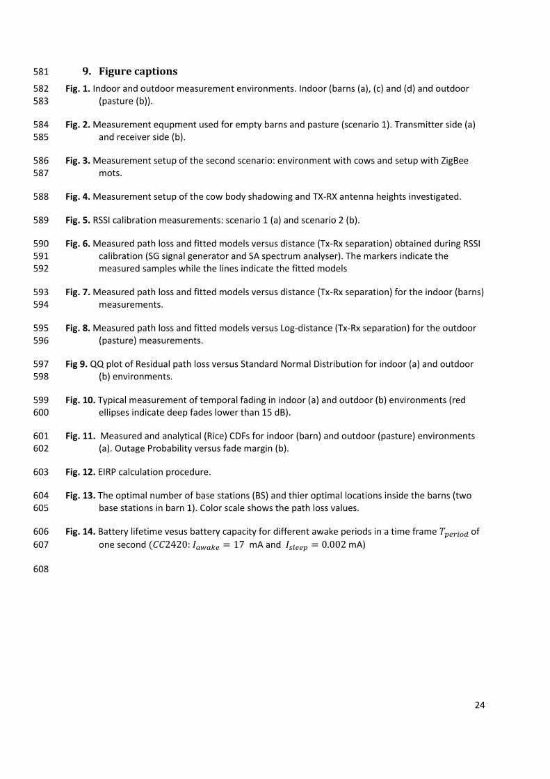
3.1 Measurement environments 145

Indoor measurements were carried out inside three barns. First, a modern barn of the Institute for 146

Agricultural and Fisheries Research (ILVO), Melle, Belgium (Fig. 1-a) was considered. This barn, which 147

7

houses approximately 144 lactating dairy cows, contains 2 milking robots, a conventional milking 148

parlour, concentrate feeders and several features enabling experimental setups. Inside the barn, four 149

similar areas are dedicated for cows lying down. These four areas have the same size and topology. 150

Therefore, measurements were performed in one single area. Each area is about 29x9 m2 and of 151

consists of 32 cubicles. Second, indoor measurements were conducted inside two other barns (UGent- 152

Biocentrum Agrivet, Melle, Belgium) as shown in Fig. 1 (c) and (d). The dimensions of barns 2 and 3 153

were 42x26 m2 and 37x21.5 m2, respectively. As barn 1, barn 2 (Fig. 1-c) is dedicated for dairy cows 154

and contains concentrate feeders and one milking robot. However, barn 3 (Fig. 1-d) is a new calf barn 155

that can accommodate about 100 animals of different ages (from the first day until the age of two 156

years when they calve for the first time). For each of these ages, appropriate boxes (individually or in 157

groups on straw and slatted floor with mats and mattresses) are provided. 158

The second investigated off-body wireless communication environment was outdoor. Outdoor 159

measurements were conducted in a pasture (Fig. 1-b) of about 33x15 m2 near the ILVO barn. All 160

measurements were carried out in the 2.4 GHz band in three barns and a pasture. The 2.4 GHz band 161

was selected because it is freely available and most practical existing technologies for WSNs work in 162

this band. 163

164

3.2 Measurement setup 165

The physical modelling of the off-body wireless channel includes different parameters. In the present 166

work, we focused on the following aspects. First, the large-scale fading due to the physical 167

environment, which is characterised by the variation of the path loss with the distance. Then, the 168

specific shadowing introduced by one cow’s body. Finally, the variation of the wireless channel over 169

time (i.e., temporal fading). 170

171

3.2.1 Large-scale fading measurements 172

8

To characterise the large-scale fading of the wireless channel, experiments were performed in both 173

indoor (barns) and outdoor (pasture) environments. For each environment, two scenarios were 174

performed, namely: without and with cows. In the first scenario, reference measurements were done 175

in empty (without cows) barns and on an empty pasture. These experiments allowed a characterisation 176

of the environments without the influence of the cows. Later, measurements with cows (second 177

scenario) determined how much the random presence of the cows affects the wireless 178

communication. 179

180

Fig. 2 shows the measurement equipment of the first scenario. The transmitter part (Fig. 2-a) consists 181

of a transmitting antenna (TX) and a signal generator. As the TX, an omnidirectional vertically polarized 182

antenna of type Jaybeam MA431Z00 (2.4 GHz, 4.2 dBi) was used. The TX antenna was mounted on a 183

plastic mast with an adjustable height. The TX antenna was connected to the Rohde & Schwarz 184

SMB100A (100 kHz - 12.75 GHz) signal generator used to inject a continuous wave signal at 2.4 GHz 185

with a constant power of 18 dBm. The receiver part (Fig. 2-b) consists of a receiving antenna (Rx) 186

mounted on a telescopic mast. At the Rx, an omnidirectional antenna of the same type as the TX was 187

used. The Rx antenna was connected to a Rohde & Schwarz FSL6 (9 kHz - 6 GHz) spectrum analyser, 188

which samples the received power level at the transmitting frequency. Sampled power values were 189

stored on a laptop through a General Purpose Interface Bus (GPIB) connection. The spectrum 190

analyser’s frequency span was set to 100 kHz. The resolution and video bandwidth were set to 3 kHz 191

and 30 kHz, respectively. According to (Tanghe et al., 2008), the resolution bandwidth has the largest 192

effect on the measured power. However, the video bandwidth has a negligible effect. The use of a 193

resolution bandwidth of 3 kHz is justified also in this paper by the small bandwidth of the continuous 194

wave signal. 195

Fig. 1 shows the transmitter and the receiver locations inside the barns and on the pasture. In the first 196

barn (Fig. 1-a), the receiver was fixed at the front right of the concerned area with an antenna height 197

9

of 4.5 m, which is a typical height of the access points. Then, the position of the transmitter was set 198

inside each box to a height ℎ𝑡𝑥 of 0.9 m above the ground. This TX height is comparable to the height 199

of a cow’s neck. The width of each box is 1.15 m. Measurements were performed for a range of 200

distances (TX-RX separation) between 7 m (nearest box) and 27 m (far box). The same TX and RX 201

heights were considered for barns 2 and 3. Inside barn 2, measurement were performed for a range 202

of distances between 4 m and 40 m. This range was 4 to 36 m for barn 3. For the outdoor 203

measurements, the receiver was fixed at the corner of the pasture, also at a height of 4.5 m. Different 204

positions of the transmitter were taken then as follows. The pasture was divided into three paths 205

separated by a distance of 4 m. Each path was divided into different measurement locations with a 206

separation of 2.5 m. Similarly to indoor environment, the height of the transmitter was set at 0.9 m. 207

The range of distances between the transmitter and the receiver was 6 to 29 m. 208

At each measurement location (indoor and outdoor), 200 samples were recorded with a sampling rate 209

of about 7 samples per second. The position of the transmitting antenna was changed a few 210

wavelengths around each measurement location (about 10 wavelengths) to obtain an average 211

received power. 212

213

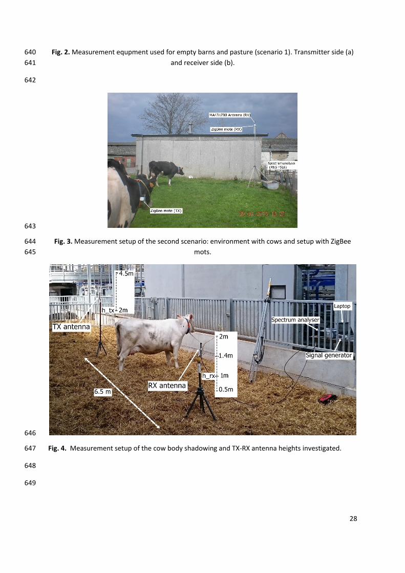
In the second scenario, the signal generator was removed and one cow was wearing a ZigBee mote 214

while fifteen other cows (indoor) and eight cows (outdoor) were moving freely inside the 215

measurement area. The ZigBee mote was configured as a transmitter and it was attached to the collar 216

around the cow’s neck (See Fig. 3). The ZigBee mote antenna separation from the cow body was fixed 217

to 5 cm. The ZigBee mote was attached to the collar because the data measured in different parts of 218

the cow’s body (e.g., leg, ear, udder) could be be gathered by a collector placed on the cow’s neck, and 219

then, transmitted to the base station. The same receiver as during the first scenario was used 220

(MA431Z00 antenna connected to spectrum analyser). In addition, a second ZigBee mote was added 221

at the same height and location as the receiving antenna. This ZigBee mote reports 150 Received Signal 222

10

Strength Indicator (RSSI) values for each measurement location by receiving the packets transmitted 223

by the other mote. The transmitting ZigBee mote (TX) was an XBee S2 (XB24-Z7WIT-004) module with 224

an omnidirectional monopole antenna (integrated whip, 1.5 dBi). The receiving ZigBee mote (RX) was 225

a RM090 module with a PCB F-antenna (1 dBi). During all measurements, the antennas were vertically 226

polarised. Fig. 3 shows an example of a measurement on the pasture. The spectrum analyser and the 227

ZigBee mote (RX) receive in parallel the signal and packets sent by the ZigBee mote (TX). The cow 228

wearing the ZigBee mote was placed at the same transmitter positions as for scenario 1. 229

3.2.2 Maximal cow body shadowing by other cows 230

In realistic cases, the communication between the on-cow device and the back-end access point will 231

be susceptible to frequent signal blocking events not only caused by the body of the cow wearing the 232

transmit node, but also by other cows, which can obscure the dominant signal path between the 233

transmitter and the receiver. In wireless communications, this well-known phenomenon is referred to 234

as body shadowing. 235

In order to quantify the impact of the cow body shadowing, a dairy cow was used and shadowing 236

measurements were conducted in an area of about 12x6 m2 inside the ILVO barn. As shown in Fig. 4, 237

the dairy cow was standing between the transmitter and the receiver. 238

The distance between the transmitter and the receiver was set to 6.5 m. This distance is sufficient to 239

be in the far-field conditions (Balanis, 2005). Then, different TX and RX antenna heights were 240

investigated as shown in Fig. 4: 2 m and 4.5 m for the transmitter and 0.5 m, 1 m, 1.4 m, and 2 m for 241

the receiver. The heights of the TX were chosen as the typical heights of the access point. However, 242

the RX heights were chosen with respect to the cow’s neck when the cow is standing, grazing, or lying 243

down. Also, to account for just the cow body shadowing, measurements were performed first without 244

cow. 245

3.2.3 Temporal fading 246

The temporal fading measurements were conducted in indoor and outdoor environments (barn 1 and 247

pasture as described in Section 3.2.1) using the same equipment as in scenario 1 (see Fig. 2). However, 248

11

the transmitter and receiver were set in stationary positions with a line of sight (LOS) condition at the 249

beginning of the experiment. The antenna heights were ℎ𝑡𝑥 = 0.9 𝑚 and ℎ𝑟𝑥 = 4.5 𝑚. These 250

scenarios were set to allow the recording of received signal power variations due to the movements 251

of the cows. For both indoor and outdoor environments, received power was recorded during 20 min, 252

including both LOS and Non-LOS (NLOS) conditions depending on the cows’ movement. The received 253

power was logged at a rate of approximately 20 samples per second. Thus, 24,000 received power 254

samples were recorded in each environment. 255

3.3 RSSI calibration 256

The RSSI reported by the receiving ZigBee mote (off-cow) is just an indication (represented by a 257

number) of the power level being received by the antenna. Thus, a calibration of the ZigBee mote using 258

the spectrum analyser (SA) has been done to determine the shift constant between the RSSI and the 259

radio-frequency (RF) power. For this aim, two experiments were performed as shown in Fig. 5. 260

In the first experiment (Fig. 5-a), a ZigBee mote was configured as a coordinator which constantly 261

broadcasts packets (Transmitter). Then, two receivers were used to sense the received power. The first 262

receiver was another ZigBee mote configured as a sniffer to capture broadcast signals (scenario 1 263

ZigBee-ZigBee). The second receiver comprised a spectrum analyser (R&S FSL6) connected to a 264

MA431Z00 antenna (scenario 1 ZigBee-SA). The antenna and ZigBee motes were placed 1 m above the 265

ground. The sniffer was used to avoid acknowledgment packets, which can affect the received power 266

of the spectrum analyser. For different distances between the transmitter and the receivers, the RF 267

power measured by the spectrum analyser and the RSSI reported by the ZigBee mote were logged 268

using laptops. 269

In the second experiment (Fig. 5-b), the ZigBee motes were removed and the signal generator (SG) 270

connected to the MA431Z00 antenna was used at the transmitter side. The same antenna type was 271

used connected to the spectrum analyser (scenario 2 SG-SA). As in Section 3.2.1, the span of the 272

spectrum analyser was set to 100 kHz. The resolution and video bandwidths were set to 3 kHz and 30 273

kHz, respectively. Exactly the same locations were measured as for the first experiment. In this way, 274

12

the RSSI values reported by the ZigBee motes were calibrated with the SA equipment in actual power 275

values (dBm or mW). In order to determine the relationship between the RSSI reported by the ZigBee 276

mote and the RF power measured by the spectrum analyser, the path loss models of the calibration 277

scenarios explained above were plotted in Fig 6, making use of equation (2). This figure shows that the 278

path loss model (red line) obtained from the RSSI values reported by the ZigBee mote is 8 dB higher 279

than the path loss model obtained from the received power of the spectrum analyser (dashed lines). 280

Also, the path loss models signal generator- spectrum analyser (SG-SA) and ZigBee-spectrum analyser 281

(ZigBee-SA) are perfectly matched. 282

Table 1 lists the parameter values of RSSI calibration path loss models. The path loss at the reference 283

distance 𝑃𝐿(𝑑0 = 1 𝑚) was approximately the same (about 41 dB) for both scenarios ZigBee-SA and 284

SG-SA. However, it shifted to 49 dB in the ZigBee-ZigBee scenario. The path loss exponents and the 285

standard deviations were nearly the same for all scenarios. In conclusion, a constant shift of 8 dB will 286

be considered between the 𝑅𝑆𝑆𝐼 reported by ZigBee mote and the RF power 𝑃𝑅𝐹 (measured by the 287

spectrum analyser as follows: 288

𝑃𝑅𝐹[𝑑𝐵𝑚] = 𝑅𝑆𝑆𝐼 − 8 𝑑𝐵 (6) 289

4. Results and discussion 290

4.1 Path loss models 291

4.1.1 Indoor path loss models 292

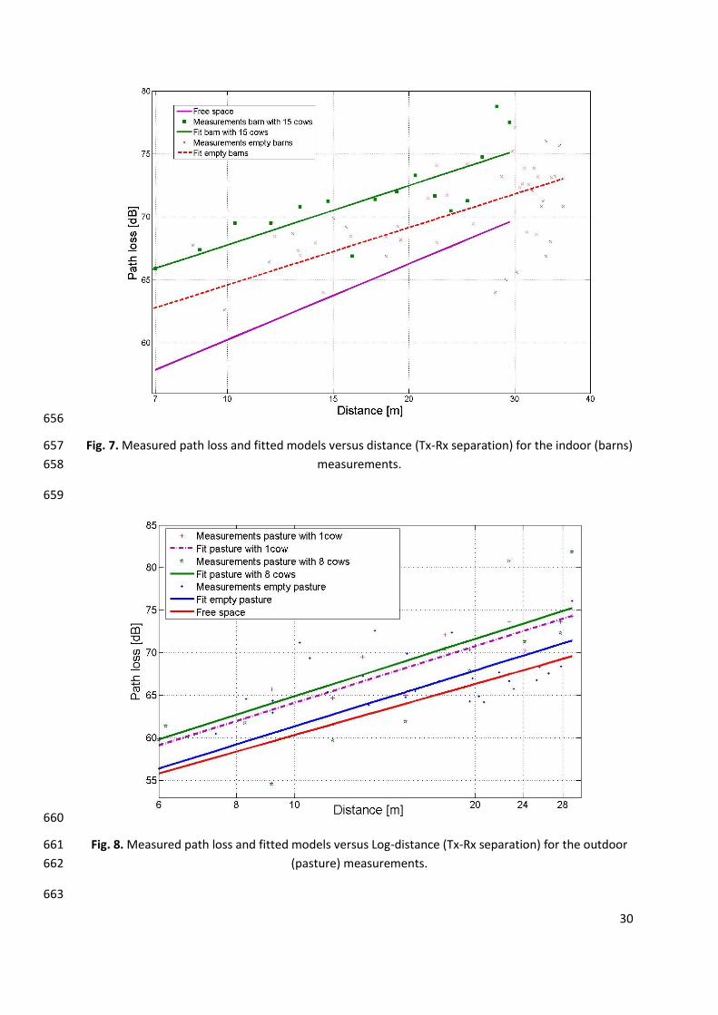
Fig. 7 shows the path loss values obtained by measurements and the fitted models versus log-distance 293

(Tx-Rx separation) for the barns. The markers indicate the individual measurements, while the lines 294

represent the path loss models obtained through fitting of the measurement data. As expected, the 295

path loss inside the empty barns was lower than the path loss when the barn contains cows (3 dB). 296

This is due to the cow’s body shadowing (the cow wearing the mote and the other cows). Table 2 lists 297

the parameter values of the obtained path loss models. The aim of the measurements performed 298

inside the barns 2 and 3 was to validate the results of the barn 1. As shown in table 2, an excellent 299

13

agreement between the path loss model parameters was obtained. Table 2 lists also the equivalent 300

path loss model gathering the obtained data from all barns. All path loss exponents were lower than 301

free space (𝑛 =2) due to the presence of multipath influence inside the barn. Similar path exponents 302

were found by (Tanghe et al., 2008) in indoor industrial environments at 2.4 GHz. The standard 303

deviations were 1.5 dB and 2.8 dB for the empty barns and barn with cows, respectively. This indicates 304

a slightly higher degree of shadow fading due to the presence of cows inside the barn. The coefficient 305

of determination 𝑅2 measures how well the path loss model (regression line) approximates the real 306

data points (measured path losses). It is defined as the square of the correlation between the 307

measured and the predicted path losses (Wang et al., 2012). As shown in Table 2, coefficients of 308

determination greater than 0.7 were obtained in both path loss models, indicating that the log-normal 309

path loss model perfectly fits the measured data. 310

4.1.2 Outdoor path loss models 311

Path loss models for the pasture are shown in Fig. 8. The difference between the empty pasture and 312

the pasture with cows is the same as the indoor (barns) case (3 dB). Table 3 lists the parameters of the 313

path loss models obtained in the outdoor pasture environment. The path loss exponents are higher 314

than for the barns (𝑛 =1.70) due to the rural environment (pasture), which is characterised by less 315

influence of multipath components (less reflecting metal materials in comparison to the barns). The 316

path loss difference between one cow and eight cows on the pasture is 0.5 dB (See Fig. 8). This means 317

that the body of the cow wearing the node is the main reason of the path loss decrease. This is due to 318

the high height of the base station (4.5 m), which makes the communication between the on-cow node 319

and the base station either in LOS conditions or obscured just by the body of the cow wearing the 320

node. Similar to the case of the indoor, the coefficients of determination (Table 3) of the outdoor are 321

also greater than 0.7, meaning that the measured data is perfectly fitted by the predicted models. 322

To verify that the path loss variations indeed follow the log-normal distribution used to fit the 323

measured path loss values, the predicted path loss is subtracted from the corresponding measured 324

path loss samples. Then, this residual path loss is used as a parameter for the Quantile-Quantile (Q-Q) 325

14

plot (Wilk and Gnanadesikan, 1968). Fig. 9 shows the Q-Q plot of residual path loss in indoor (barns) 326

and outdoor (pasture) environments versus the standard Gaussian distribution. Fig. 9 aggregates all 327

residuals path loss values of indoor scenarios (a) and outdoor scenarios (b). As shown in Fig. 9, the 328

residual path loss matches well the Gaussian distribution, although there are some small deviations in 329

the tails. 330

4.2 Cow body shadowing 331

The obtained values of the cow body shadowing for different TX and RX heights are listed in Table 4. 332

The cow body shadowing varies from 1 dB to 7 dB. In general, the shadowing increases when the height 333

of the TX and/or the RX decreases. This can be explained as follows. With high ℎ𝑇𝑋 and ℎ𝑅𝑋, the 334

transmitter and the receiver are in LOS condition and just a part of the power is shadowed by the cow 335

body (e.g., 1 dB for ℎ𝑇𝑋 = 4.5 m and ℎ𝑅𝑋 = 2 m, Table 4). However for low ℎ𝑇𝑋 and ℎ𝑅𝑋, the 336

communication is totally obscured by the cow body (e.g., 7.4 dB for ℎ𝑇𝑋 = 2 m and ℎ𝑅𝑋 = 0.5 m). This 337

validates the result obtained in Section 4.1.2 (ℎ𝑇𝑋 = 1 m and ℎ𝑅𝑋 = 4.5 m), where the body of the 338

cow wearing the node was the main reason of the path loss decrease and the other cows had less 339

influence (0.5 dB). 340

4.3 Temporal fading 341

4.3.1 Rician K-factor 342

Fig. 10 shows a typical temporal fading measurement of received power (around median) in dB over 343

time in min, executed in indoor (a) and outdoor (b) environments. Deep fades of 15 dB (15 dB below 344

the median power) occurred several times in the barn (indoor) between 6 and 8 min, as indicated by 345

the red ellipses in Fig. 10. However, this occurred only once on the pasture at the instant t=3 min. This 346

indicates that there are more fading events in barns compared to pastures especially when the cows 347

come close to the antennas. The deep fades all have a short duration, which would very unlikely 348

substantially impair communication between cow nodes and access points. 349

For each environment, the Rician K-factor is estimated based on the moment method presented in 350

Section 3.2. This method estimates the K-factor directly from the measured samples without need for 351

15

a curve fitting operation. A K-factor of 10 dB was obtained in the barn and 13 dB in the pasture. These 352

large values indicate a strong specular path LOS component in our measurements due to the TX height 353

(4.5 m). The barn (indoor) K-factor (K=10) is lower than for pasture (K=13), meaning that the 354

contribution of multipath propagation is higher inside the barns in comparison to the pasture. 355

4.3.2 Cumulative distribution function 356

The probability that the received power does not exceed a given threshold is determined by the 357

integration of the PDF and is called cumulative distribution function (CDF). Fig. 11-a shows the 358

measured and the analytical (Rice) CDF for the two investigated environments. As shown in this figure, 359

the CDFs in the considered barns and pastures environments follow a Rician distribution. 360

4.3.3 Fade margin 361

The obtained K-factors (Section 4.3.1) and the corresponding CDFs (Section 4.3.2) are used to calculate 362

a fade margin associated with temporal fading for a given outage probability. The outage probability, 363

which determines the probability that the wireless system will be out of the service (quality of service 364

not reached) and the corresponding fade margin will be used in the link budget calculation for the 365

network planning application of Section 5. 366

The details of the calculation are explained in (Andreas, 2011). Fig. 11-b shows the outage probability 367

versus the fade margin in dB. For an outage probability of 0.01 (99% of the time, the variation around 368

the median will not exceed the fade margin), a fade margin of 4 dB in pastures and 6 dB in barns should 369

be considered in the link budget analysis. 370

5. Application: Network planning 371

The primary goal of network planning is to provide connectivity, or in other words coverage at all 372

desired locations. Wireless connectivity is determined by a number of parameters such as wireless 373

channel characteristics, the number of receiving nodes, their locations, and the effective isotropic 374

radiated power (EIRP) of the sensor nodes. 375

16

In this Section, a ZigBee-based WSN is proposed for the healthcare monitoring of dairy cows. In this 376

network, the on-cow sensor nodes are considered as end nodes and the ZigBee sinks as coordinators. 377

The results and models presented above (Section 4) and the CC2420 chip specifications (CC2420 378

Datasheet, Texas Instruments 2013) are used to predict and optimise the number of sinks, their 379

locations and power, and the EIRP of the on-cow nodes inside the barns, based on the WiCa Heuristic 380

Indoor Propagation Prediction (WHIPP) tool (Plets et al., 2012). This tool has proven its use for the 381

accurate coverage prediction and optimisation in indoor environments and for optimal network 382

planning. 383

5.1 Planning tool 384

The WHIPP tool uses a heuristic planning algorithm, developed and validated for the prediction and 385

optimisation of wireless coverage in indoor environments. The tool is constructed as a web service, 386

which allows importing an existing floor plan in different formats or drawing a floor plan of a building, 387

where the user can choose between different wall materials. The web service transfers this floor plan 388

to a Java backend, after which the server predicts throughput and path loss, based on the path loss 389

model entered by the user. The drawing tool then superimposes this output over the floor plan with a 390

colour code. This gives the user a clear view on the estimated wireless connection quality (coverage) 391

in each area (Plets et al., 2010). 392

5.2 Planning parameters 393

After importing the ground plan of the barns, the network parameters and requirements should be 394

defined carefully for an accurate network planning. Table 5 summarises the parameters used for the 395

calculations. Like in the measurements, the transmitter and receiver antenna heights were set to 4.5 396

m and 1.0 m, respectively. A data rate of 250 kbps was used, which corresponds to the maximum 397

physical data rate of the ZigBee mote (Road and Minnetonka, 2009). The path loss model obtained 398

inside the barns with 15 cows is considered (Table 5). The shadowing margin is determined such that 399

95% of the locations inside the barn are covered by the wireless system. This margin is derived from 400

17

the standard deviation 𝜎 around the path loss model (Section 4.4.1) and equals 1.65𝜎. The fade margin 401

obtained inside the barns is considered (See Fig 11-b). All relevant parameters are listed in Table 5. 402

5.3 Required on-cow node EIRP 403

The procedure to determine the minimum EIRP required for the uplink (on-cow sensor to sink) wireless 404

connection is presented in Fig. 12. First, the WHIPP tool is used to determine the optimal number and 405

location of the sinks inside the barns given the ground plan of the barn, the base station EIRP, the 406

node’s sensitivity, and the path loss model parameters (Section 4.1.1). Based on the optimal placement 407

of the sinks, the maximal path loss between a base station and an on-cow node is determined by the 408

tool. The minimum EIRP required for the uplink connection (sensor node’s EIRP) is derived from the 409

maximal path loss and the sensitivity of the sink (base station). 410

The required number of base stations inside the barn 1 was 1, 2, or 3, depending on the EIRP of the 411

base station. However, barns 2 and 3 have smaller dimensions in comparison to barn 1. Therefore, the 412

required number of base stations was always one (independent of the coordinator’s EIRP). Fig. 13 413

shows the optimal design of the base station network for the three barns (case of two base stations in 414

barn 1). The colour scale illustrates the path loss values between each location and the nearest base 415

station. This maximal path loss value is used to derive the minimally required on-cow node EIRP 416

(𝐸𝐼𝑅𝑃𝑛𝑜𝑑𝑒𝑚𝑖𝑛 ) as follows: 417

𝐸𝐼𝑅𝑃𝑛𝑜𝑑𝑒𝑚𝑖𝑛 = 𝑃𝑠𝑒𝑛𝑠

𝐵𝑆 + 𝑃𝐿𝑚𝑎𝑥 + 𝑀𝐹 + 𝑀𝑆ℎ (7) 418

where 𝑃𝑠𝑒𝑛𝑠𝐵𝑆 is the base station sensitivity [dBm], 𝑃𝐿𝑚𝑎𝑥 the maximal path loss [dB], 𝑀𝐹 the fade 419

margin [dB], and 𝑀𝑆ℎ the shadowing margin [dB]. Table 6 lists the minimally required on-cow EIRP for 420

the three investigated barns for different sizes of the base station set. The calculations were performed 421

using the specifications of CC2420 chip (CC2420 Datasheet, Texas Instruments 2013). For barn 1, the 422

sensor node’s required EIRP varies between -9.5 dBm and -0.4 dBm depending on the number of base 423

stations, which is related to their EIRP. As this EIRP increases, the required number of base stations 424

decreases and the maximal path loss increases. Thus, the sensor node’s EIRP has to increase to 425

maintain a connection. The obtained on-cow node EIRPs for barn 2 and barn 3 were -6.7 dBm and -7.0 426

18

dBm, respectively. These values are lower than the transmit power provided by the specifications 427

(Zigbee Alliance, 2011), which means that power consumption reduction can be achieved to increase 428

the battery lifetime of the sensor node (Section 5.5). We note that the number of cows that can be 429

served inside each barn depends on many parameters such as the access method (MAC layer), data 430

load, number of base stations, and the nature of the data to be transferred (critical or non-critical). For 431

example, critical data requires rapid intervention of the farmer and thus real-time updating is required. 432

An on-cow node is covered by the wireless network if its transmitted signal reaches the base station 433

antenna with a power higher than the base station sensitivity. As shown in Table 6, the maximal path 434

loss is lower than 84 dB inside the three barns. Considering an 𝐸𝐼𝑅𝑃𝑛𝑜𝑑𝑒 of 3 dBm, a base station 435

sensitivity of -95 dBm, a fade margin of 6 dB (Fig. 11-b), and a shadowing margin of 5 dB (see Table 5), 436

then, a path loss 𝑃𝐿 of 84 dB indicates that this location is covered. Therefore, the three barns are 437

indeed totally covered. 438

5.4 Power consumption analysis and battery lifetime of sensor node 439

One of the key factors in determining the success of a WSN is the battery lifetime of the sensor nodes. 440

Since the battery of the sensor node is a limited resource in any WSN, an accurate network planning 441

should optimize the power consumption in order to make the network operational as long as possible. 442

The battery lifetime in hours of the sensor node is estimated as a function of the battery capacity in 443

mAh and the node’s activity (awake and sleep periods) as follows: 444

𝐵𝑎𝑡𝑡𝑒𝑟𝑦 𝑙𝑖𝑓𝑒𝑡𝑖𝑚𝑒 =𝐵𝑎𝑡𝑡𝑒𝑟𝑦 𝑐𝑎𝑝𝑎𝑐𝑖𝑡𝑦

(𝐼𝑎𝑤𝑎𝑘𝑒 . 𝑇𝑎𝑤𝑎𝑘𝑒 + 𝐼𝑠𝑙𝑒𝑒𝑝. 𝑇𝑠𝑙𝑒𝑒𝑝)(𝑇𝑎𝑤𝑎𝑘𝑒 + 𝑇𝑠𝑙𝑒𝑒𝑝) (8) 445

where 𝐼𝑎𝑤𝑎𝑘𝑒 and 𝐼𝑠𝑙𝑒𝑒𝑝 are the current consumptions in mA of the sensor node during the awake 446

period 𝑇𝑎𝑤𝑎𝑘𝑒 (transmitting or receiving data) and the sleep period 𝑇𝑠𝑙𝑒𝑒𝑝in seconds, respectively. The 447

battery lifetime was calculated based on the current consumption of CC2420 chip. According to 448

(CC2420 Datasheet Texas Instruments 2013), 𝐼𝑎𝑤𝑎𝑘𝑒 varies between 8.5 mA (for -25 dBm transmit 449

power) and 17.4 mA (for 0 dBm transmit power). During the sleep period, the CC2420 chip 450

consumes 𝐼𝑠𝑙𝑒𝑒𝑝 = 0.002 mA. The total period 𝑇𝑝𝑒𝑟𝑖𝑜𝑑 = 𝑇𝑎𝑤𝑎𝑘𝑒 + 𝑇𝑠𝑙𝑒𝑒𝑝 can be configured 451

19

depending on the WSN application. In our calculations, a realistic value of 1 second for 𝑇𝑝𝑒𝑟𝑖𝑜𝑑 was 452

used. Like in (Kwong et al., 2012), battery capacities between 1000 mAh and 5000 mAh were 453

investigated. 454

Fig. 14 shows an example of calculation of the battery lifetime as a function of the battery capacity for 455

different awake periods when 𝐼𝑎𝑤𝑎𝑘𝑒 = 17.4 mA (0 dBm transmit power). The percentage values 456

indicate the ratio 𝑇𝑎𝑤𝑎𝑘𝑒/𝑇𝑝𝑒𝑟𝑖𝑜𝑑. The battery lifetime increases as the capacity increases. Also, the 457

battery lifetime increases as the awake period decreases. The awake period determines the amount 458

of data that can be transmitted per time unit (1 second). For 𝑇𝑎𝑤𝑎𝑘𝑒 = 5 ms and a throughput of 250 459

kbps, 1250 bits can be transmitted every second. In this situation, a battery capacity of about 3000 460

mAh results in a lifetime of about three years. This is an acceptable lifetime, considering the average 461

lifetime of a cow (5 years) and the fact that most cows’ anomalies (e.g., mastitis, heat, lameness) occur 462

after the first calving (around second year).Therefore, the cows can be equipped with the healthcare 463

monitoring system during three years. 464

To estimate the battery lifetime of the on-cow nodes for the three investigated barns, the obtained 465

on-cow EIRP (Section 5.4) are considered with a typical battery capacity of 3000 mAh (Kwong et al., 466

2012). Since the transmit power of the CC2420 chip varies between -25 dBm and 0 dBm with a step of 467

5 dBm, each on-cow EIRP (Table 6) is related to the required output power level. Table 7 lists the 468

obtained battery lifetimes for a varying node activity (awake period). In fact, there is a trade-off 469

between the battery lifetime and the node activity. As the activity increases, which is related to the 470

network applications, the battery lifetime decreases. If the data load required for each cow is 471

determined (this depends on the monitored parameters e.g., cow movement, temperature, drinking 472

and eating time), Table 7 can be used then to estimate the battery lifetime for a given on-cow EIRP. 473

In case of applications that require more throughput, the awake period should be higher, decreasing 474

the battery lifetime. In such situations, wireless charging of the nodes using an inductive powering 475

system (Thoen and Stevens, 2015) can be used to avoid a costly and labour intensive battery 476

20

replacement procedure. The inductive powering elements can be installed at the drinking places, so 477

that during the time slots when the cow is drinking the power can be wirelessly transferred to the 478

node’s battery. Finally, we note that the battery lifetime calculation presented in this paper provides 479

an estimation depending upon the considered battery technology, connected peripherals, and 480

required duty cycles for each particular application. 481

6. Conclusions and future work 482

The off-body wireless channel between a node placed on the body of a dairy cow and an access point 483

inside barns and on pastures has been characterised at 2.4 GHz. The reliability of this wireless 484

connection is a key factor for the success of a cow healthcare monitoring system that facilitates herd 485

management and cow welfare. Three different barns and a pasture have been investigated. 486

Measurements of large-scale fading, cow body shadowing, and temporal fading have been performed 487

with spectrum analysis and ZigBee motes equipment. Results have shown that the large-scale fading 488

can be well described by a one-slope log-normal path loss model. In line-of-sight conditions, the 489

highest path loss increase resulted from the body of the cow wearing the sensor node (3 dB). However, 490

the other cows had less influence (0.5 dB). A cow body shadowing between 1 dB and 7 dB was 491

obtained, depending on the transmitter and receiver heights. The temporal fading was statistically 492

described by Rician distributions. The fading occurrences and depth were higher inside the barns than 493

on the pasture. Consequently, the fade margins were 6 dB and 4 dB for the barns and pasture, 494

respectively. The obtained wireless channel characteristics were then used to optimise the number of 495

the base stations, their EIRP, and their locations inside the investigated barns, based on the WHIPP 496

prediction tool. Assuming typical specifications for the sensor nodes, different network designs were 497

proposed, each with a different impact on the minimal on-cow node transmit power and lifetime. The 498

battery lifetime of the sensor nodes was estimated as a function of the battery capacity, the network 499

design, and the sensor’s activity. Battery lifetimes between 143 and 2193 days were obtained 500

depending on the network design and application. 501

21

As future research topic, multiple health parameters will be collected from different parts of the cow’s 502

body. For example, data from legs, ear, and udder can be transferred to a data collector placed on the 503

cow’s neck and then forwarded to the access point. Therefore, future work will investigate the on-504

body wireless communication between two nodes placed on the cow’s body (e.g., leg to neck, udder 505

to neck, and ear to neck). 506

7. Acknowledgments 507

This work was supported by the iMinds-MoniCow project, co-funded by iMinds, a research institute 508

founded by the Flemish Government in 2004, and the involved companies and institutions. E. Tanghe 509

is a Post-Doctoral Fellow of the FWO-V (Research Foundation-Flanders). The authors would like to 510

thank Thijs Decroos, Sara Van Lembergen, and Matthias Van den Bossche for their help during the 511

measurements. The authors would like to thank also ILVO and UGent- Biocentrum Agrivet for 512

providing the barns for the measurements. 513

8. References 514

Abdi, A., Tepedelenlioglu, C., Kaveh, M., Giannakis, G., 2001. On the estimation of the K parameter 515

for the rice fading distribution. IEEE Commun. Lett. 5, 92–94. doi:10.1109/4234.913150 516

Akyildiz, I., Su, W., Sankarasubramaniam, Y., Cayirci, E., 2002. Wireless sensor networks: a survey. 517

Comput. Networks 38, 393–422. doi:10.1016/S1389-1286(01)00302-4 518

Alemdar, H., Ersoy, C., 2010. Wireless sensor networks for healthcare: A survey. Comput. Networks 519

54, 2688–2710. doi:10.1016/j.comnet.2010.05.003 520

Andonovic, I., Michie, W., Gilroy, M.P., Goh, H.G., Kwong, K., Sasloglou, K., Wu, T.-T., 2010. Wireless 521

sensor networks for cattle health monitoring. Online 84–89. 522

doi:10.1109/MOBIQUITOUS.2005.65 523

Andreas, M.F., 2011. Wireless Communications, second. ed, Wiley Publishing. 524

doi:10.1002/9781119992806.fmatter 525

Balanis, C.A., 2005. Antenna theory: Analysis and design, 3rd ed, Wiley. 526

Barkema, H.W., Westrik, J.D., van Keulen, K.A.S., Schukken, Y.H., Brand, A., 1994. The effects of 527

lameness on reproductive performance, milk production and culling in Dutch dairy farms. Prev. 528

Vet. Med. doi:10.1016/0167-5877(94)90058-2 529

Bernadó, L., Zemen, T., Member, S., Tufvesson, F., Member, S., Molisch, A.F., Mecklenbräuker, C.F., 530

Member, S., 2015. Time- and Frequency-Varying K -Factor of Non-Stationary Vehicular Channels 531

for Safety-Relevant Scenarios. IEEE Trans. Intell. Transp. Syst. 16, 1007–1017. 532

22

CC2420 Datasheet Texas Instruments 2013, n.d. 2.4 GHz IEEE 802.15.4 / ZigBee-ready RF Transceiver, 533

downloadable at www.chipcon.com. 534

Huircán, J.I., Muñoz, C., Young, H., Von Dossow, L., Bustos, J., Vivallo, G., Toneatti, M., 2010. ZigBee-535

based wireless sensor network localization for cattle monitoring in grazing fields. Comput. 536

Electron. Agric. 74, 258–264. doi:10.1016/j.compag.2010.08.014 537

Kahn, J.M., Katz, R.H., Pister, K.S.J., 2000. Emerging Challenges: Mobile Networking for Smart Dust. J. 538

Commun. Networks 2, 188–196. 539

Kwong, K.H., Andonovic, I., Wu, T.-T., Goh, H.G., Sasloglou, K., Stephen, B., Glover, I., Shen, C., Du, 540

W., Michie, C., 2012. Practical considerations for wireless sensor networks in cattle monitoring 541

applications. Comput. Electron. Agric. 81, 33–44. doi:10.1016/j.compag.2011.10.013 542

Lee, W.C.Y., 1985. Estimate of local average power of a mobile radio signal. IEEE Trans. Veh. Technol. 543

34. doi:10.1109/T-VT.1985.24030 544

Mayer, K., Ellis, K., Taylor, K., 2004. Cattle health monitoring using wireless sensor networks.pdf. 545

Nadimi, E.S., Jørgensen, R.N., Blanes-Vidal, V., Christensen, S., 2012. Monitoring and classifying 546

animal behavior using ZigBee-based mobile ad hoc wireless sensor networks and artificial 547

neural networks. Comput. Electron. Agric. 82, 44–54. doi:10.1016/j.compag.2011.12.008 548

Nadimi, E.S., Søgaard, H.T., Bak, T., Oudshoorn, F.W., 2008. ZigBee-based wireless sensor networks 549

for monitoring animal presence and pasture time in a strip of new grass. Comput. Electron. 550

Agric. 61, 79–87. doi:10.1016/j.compag.2007.09.010 551

Parsons, J.D., 2000. The Mobile Radio Propagation Channel, Electrical Engineering. 552

doi:10.1049/ir:19920094 553

Pérez Fontán, F., Mariño Espiñeira, P., 2008. Modelling the Wireless Propagation Channel: A 554

Simulation Approach with MATLAB, Modelling the Wireless Propagation Channel: A Simulation 555

Approach with MATLAB. doi:10.1002/9780470751749 556

Plets, D., Joseph, W., Vanhecke, K., Tanghe, E., Martens, L., 2012. Coverage prediction and 557

optimization algorithms for indoor environments. EURASIP J. Wirel. Commun. Netw. 558

doi:10.1186/1687-1499-2012-123 559

Plets, D., Joseph, W., Vanhecke, K., Tanghe, E., Martens, L., 2010. Development of an accurate tool 560

for path loss and coverage prediction in indoor environments. Antennas Propag. (EuCAP), 2010 561

Proc. Fourth Eur. Conf. doi:10.1109/EUCAP.2010.5505545 562

Rappaport, T.S., 2002. Wireless communications : principles and practice, Prentice Hall 563

23

communications engineering and emerging technologies series. 564

Road, B., Minnetonka, E., 2009. XBee®/XBee-PRO® ZB RF Modules. 565

Tanghe, E., Joseph, W., Verloock, L., Martens, L., Capoen, H., Van Herwegen, K., Vantomme, W., 566

2008. The industrial indoor channel: Large-scale and temporal fading at 900, 2400, and 5200 567

MHz. IEEE Trans. Wirel. Commun. 7, 2740–2751. doi:10.1109/TWC.2008.070143 568

Thoen, B., Stevens, N., 2015. Development of a Communication Scheme for Wireless Power 569

Applications With Moving Receivers. IEEE Trans. Microw. Theory Tech. 63, 857–863. 570

doi:10.1109/TMTT.2015.2397442 571

Wang, D., Song, L., Kong, X., Zhang, Z., 2012. Near-ground path loss measurements and modeling for 572

wireless sensor networks at 2.4 GHz. Int. J. Distrib. Sens. Networks 2012. 573

doi:10.1155/2012/969712 574

Wietrzyk, B., Radenkovic, M., 2010. Realistic Large Scale ad hoc Animal Monitoring. Int. J. Adv. Life 575

Sci. 2, 1–17. 576

Wilk, M.B., Gnanadesikan, R., 1968. Probability plotting methods for the analysis of data. Biometrika 577

55, 1–17. doi:10.1093/biomet/55.1.1 578

Zigbee Alliance, 2011. ZigBee/IEEE 802.15.4 specification. 579

580

24

9. Figure captions 581

Fig. 1. Indoor and outdoor measurement environments. Indoor (barns (a), (c) and (d) and outdoor 582 (pasture (b)). 583

Fig. 2. Measurement equpment used for empty barns and pasture (scenario 1). Transmitter side (a) 584 and receiver side (b). 585

Fig. 3. Measurement setup of the second scenario: environment with cows and setup with ZigBee 586 mots. 587

Fig. 4. Measurement setup of the cow body shadowing and TX-RX antenna heights investigated. 588

Fig. 5. RSSI calibration measurements: scenario 1 (a) and scenario 2 (b). 589

Fig. 6. Measured path loss and fitted models versus distance (Tx-Rx separation) obtained during RSSI 590 calibration (SG signal generator and SA spectrum analyser). The markers indicate the 591 measured samples while the lines indicate the fitted models 592

Fig. 7. Measured path loss and fitted models versus distance (Tx-Rx separation) for the indoor (barns) 593 measurements. 594

Fig. 8. Measured path loss and fitted models versus Log-distance (Tx-Rx separation) for the outdoor 595 (pasture) measurements. 596

Fig 9. QQ plot of Residual path loss versus Standard Normal Distribution for indoor (a) and outdoor 597 (b) environments. 598

Fig. 10. Typical measurement of temporal fading in indoor (a) and outdoor (b) environments (red 599 ellipses indicate deep fades lower than 15 dB). 600

Fig. 11. Measured and analytical (Rice) CDFs for indoor (barn) and outdoor (pasture) environments 601 (a). Outage Probability versus fade margin (b). 602

Fig. 12. EIRP calculation procedure. 603

Fig. 13. The optimal number of base stations (BS) and thier optimal locations inside the barns (two 604 base stations in barn 1). Color scale shows the path loss values. 605

Fig. 14. Battery lifetime vesus battery capacity for different awake periods in a time frame 𝑇𝑝𝑒𝑟𝑖𝑜𝑑 of 606

one second (𝐶𝐶2420: 𝐼𝑎𝑤𝑎𝑘𝑒 = 17 mA and 𝐼𝑠𝑙𝑒𝑒𝑝 = 0.002 mA) 607

608

25

10. Table captions 609

Table 1. Parameter values of the path loss models. 610

𝒅𝟎[𝒎] 𝑷𝑳(𝒅𝟎) [𝒅𝑩] 𝒏[−] 𝝈[𝒅𝑩] 𝑹𝟐[−]

ZigBee-ZigBee 1 49 1.60 3.5 0.74

ZigBee- Spectrum analyser

1 41.2 1.80 3.1 0.80

Signal generator -Spectrum analyser

1 41.7 1.70 4.0 0.70

611

Table 2. Parameter values of the path loss models indoor (barns). 612

𝒅𝟎[𝒎] 𝑷𝑳(𝒅𝟎) [𝒅𝑩] 𝒏[−] 𝝈[𝒅𝑩] 𝑹𝟐[−]

Barn 1 empty 1 48.0 1.50 3.7 0.70

Barn 2 emty 1 49.8 1.58 3.8 0.78

Barn 3 empty 1 47.0 1.51 3.28 0.82

Barns empty 1 48.6 1.50 3.7 0.8

Barn 1 with 15 cows 1 52.4 1.68 2.8 0.82

613

Table 3. Parameter values of the path loss models outdoor (pasture). 614

𝒅𝟎[𝒎] 𝑷𝑳(𝒅𝟎) [𝒅𝑩] 𝒏[−] 𝝈[𝒅𝑩] 𝑹𝟐[−]

Empty pasture 1 39.5 2.18 3.8 0.73

Pasture with one cow 1 42.8 2.25 2.6 0.81

Pasture with 8 cows 1 42.4 2.3 5.3 0.71

615

Table 4. Values of the cow body shadowing. 616

Shadowing [dB] 𝒉𝑻𝑿[m]

2 4.5

𝒉𝑹𝑿[m]

0.5 7.4 4.0

1 3.7 3.1

1.4 2.8 2.4

2 1.0 1.0

617

618

619

620

621

622

623

26

Table 5. Parameters used for network planning. 624

Parameters Value Unit

Coordinator (base station)

Throughput 0.250 Mbps Sensitivity -95* dBm Elevation 4.5 m

Margins

Interference margin 0 dB Shadowing margin (95 %) 5 dB Fade margin 6 dB

Path loss model

Reference distance 1 m Reference path loss 52.4 dB Path loss exponent 1.7 [-]

End nodes (sensor nodes)

Throughput 0.250 Mbps

Sensitivity -95 dBm

Elevation 1 m

* CC2420 Datasheet, Texas Instruments, March 2013. Downloadable at www.chipcon.com 625

626

Table 6. Minimum on-cow node EIRP for the three investigated barns. 627

Base station EIRP [dBm]

Barn Number of required base stations

Maximal path loss [dB]

Minimally required on-cow node EIRP [dBm]

EIRP<0 Barn 1 3 74.5 -9.5 Barn 2 1 77.3 -6.7 Barn 3 1 77 -7.0

0<EIRP<5 Barn 1 2 79.5 -4.5 EIRP>5 Barn 1 1 83.6 -0.4

628

629

Table 7. Battery lifetime [days] estimation for different on-cow EIRP and awake periods based on 630

cc2420 power consumption and a typical battery capacity of 3000 mA. 631

Barn (number of base stations BS)

On-cow node EIRP [dBm]

Corresponding CC2420 output power [dBm]

Current Consumption (transmit mode) [mA]

Battery lifetime [days]

5 ms (0.5%)

10 ms (1.0%)

20 ms (2.0%)

50 ms (5.0%)

Barn 1 (3 BS) -9.5 -10 11 2193 1116 563 226 Barn 2 (1 BS) -6.7 -5 14 1736 880 443 178 Barn 3 (1 BS) -7.0 Barn 1 (2 BS) -4.5 Barn 1 (1 BS) -0.4 0 17 1405 710 357 143

632

633

634

27

11. Figure captions 635

636

Fig. 1. Indoor and outdoor measurement environments. Indoor (barns (a), (c) and (d) and outdoor 637

(pasture (b)). 638

639

28

Fig. 2. Measurement equpment used for empty barns and pasture (scenario 1). Transmitter side (a) 640

and receiver side (b). 641

642

643

Fig. 3. Measurement setup of the second scenario: environment with cows and setup with ZigBee 644

mots. 645

646

Fig. 4. Measurement setup of the cow body shadowing and TX-RX antenna heights investigated. 647

648

649

29

650

Fig. 5. RSSI calibration measurements: scenario 1 (a) and scenario 2 (b). 651

652

Fig. 6. Measured path loss and fitted models versus distance (Tx-Rx separation) obtained during RSSI 653

calibration (SG signal generator and SA spectrum analyser). 654

655

30

656

Fig. 7. Measured path loss and fitted models versus distance (Tx-Rx separation) for the indoor (barns) 657

measurements. 658

659

660

Fig. 8. Measured path loss and fitted models versus Log-distance (Tx-Rx separation) for the outdoor 661

(pasture) measurements. 662

663

31

664

Fig. 9. QQ plot of Residual path loss versus Standard Normal Distribution for indoor (a) and outdoor 665

(b) environments. 666

667

668

Fig. 10. Typical measurement of temporal fading in indoor (a) and outdoor (b) environments. 669

670

32

671

Fig. 11. Measured and analytical (Rice) CDFs for indoor (barns) and outdoor (pasture) environments 672

(a). Outage Probability versus fade margin (b). 673

674

Fig. 12. EIRP calculation procedure. 675

33

676

Fig. 13. The optimal number of base stations (BS) and thier optimal locations inside the barns (two 677 base stations in barn 1). Color scale shows the path loss values. 678

34

679

Fig. 14. Battery lifetime vesus battery capacity for different awake periods in a time frame 𝑇𝑝𝑒𝑟𝑖𝑜𝑑 of 680

one second (𝐶𝐶2420: 𝐼𝑎𝑤𝑎𝑘𝑒 = 17 mA and 𝐼𝑠𝑙𝑒𝑒𝑝 = 0.002 mA) 681

682

683