Experimental Characterization of Soot Formation in Diffusion Flames and Explosive Fireballs by Kevin McNesby, Barrie Homan, John Densmore, Matt Biss, Richard Benjamin, Matt Kurman, Chol-bum Kweon, Brendan McAndrew, and Zachary Quine ARL-TR-5979 April 2012 Approved for public release; distribution is unlimited.
Transcript
Experimental Characterization of Soot Formation in
Diffusion Flames and Explosive Fireballs
by Kevin McNesby, Barrie Homan, John Densmore, Matt Biss,
Richard Benjamin, Matt Kurman, Chol-bum Kweon,
Brendan McAndrew, and Zachary Quine
ARL-TR-5979 April 2012
Approved for public release; distribution is unlimited.
NOTICES
Disclaimers
The findings in this report are not to be construed as an official Department of the Army position unless
so designated by other authorized documents.
Citation of manufacturer’s or trade names does not constitute an official endorsement or approval of the
use thereof.
Destroy this report when it is no longer needed. Do not return it to the originator.
Army Research Laboratory Aberdeen Proving Ground, MD 21005-5066
ARL-TR-5979 April 2012
Experimental Characterization of Soot Formation in
Diffusion Flames and Explosive Fireballs
Kevin McNesby, Barrie Homan, John Densmore, Matt Biss, Richard
Benjamin, Matt Kurman, Chol-bum Kweon, Brendan McAndrew,
and Zachary Quine Weapons and Materials Research Directorate
Approved for public release; distribution is unlimited.
ii
REPORT DOCUMENTATION PAGE Form Approved OMB No. 0704-0188
Public reporting burden for this collection of information is estimated to average 1 hour per response, including the time for reviewing instructions, searching existing data sources, gathering and maintaining the data needed, and completing and reviewing the collection information. Send comments regarding this burden estimate or any other aspect of this collection of information, including suggestions for reducing the burden, to Department of Defense, Washington Headquarters Services, Directorate for Information Operations and Reports (0704-0188), 1215 Jefferson Davis Highway, Suite 1204, Arlington, VA 22202-4302. Respondents should be aware that notwithstanding any other provision of law, no person shall be subject to any penalty for failing to comply with a collection of information if it does not display a currently valid OMB control number.
PLEASE DO NOT RETURN YOUR FORM TO THE ABOVE ADDRESS.
1. REPORT DATE (DD-MM-YYYY)
April 2012
2. REPORT TYPE
Final
3. DATES COVERED (From - To)
September 2006–September 2010 4. TITLE AND SUBTITLE
Experimental Characterization of Soot Formation in Diffusion Flames and
Explosive Fireballs
5a. CONTRACT NUMBER
5b. GRANT NUMBER
5c. PROGRAM ELEMENT NUMBER
6. AUTHOR(S)
Kevin McNesby, Barrie Homan, John Densmore, Matt Biss, Richard Benjamin,
Matt Kurman, Chol-bum Kweon, Brendan McAndrew, and Zachary Quine
5d. PROJECT NUMBER
SERDP-1 5e. TASK NUMBER
5f. WORK UNIT NUMBER
7. PERFORMING ORGANIZATION NAME(S) AND ADDRESS(ES)
U.S. Army Research Laboratory
ATTN: RDRL-WML-C
Aberdeen Proving Ground, MD 21005-5066
8. PERFORMING ORGANIZATION REPORT NUMBER
ARL-TR-5979
9. SPONSORING/MONITORING AGENCY NAME(S) AND ADDRESS(ES)
Strategic Environmental Research and Development Program
901 North Stuart St., Ste., 303
Arlington, VA 22203
10. SPONSOR/MONITOR’S ACRONYM(S)
SERDP/DOD
11. SPONSOR/MONITOR'S REPORT NUMBER(S)
12. DISTRIBUTION/AVAILABILITY STATEMENT
Approved for public release; distribution is unlimited.
13. SUPPLEMENTARY NOTES
14. ABSTRACT
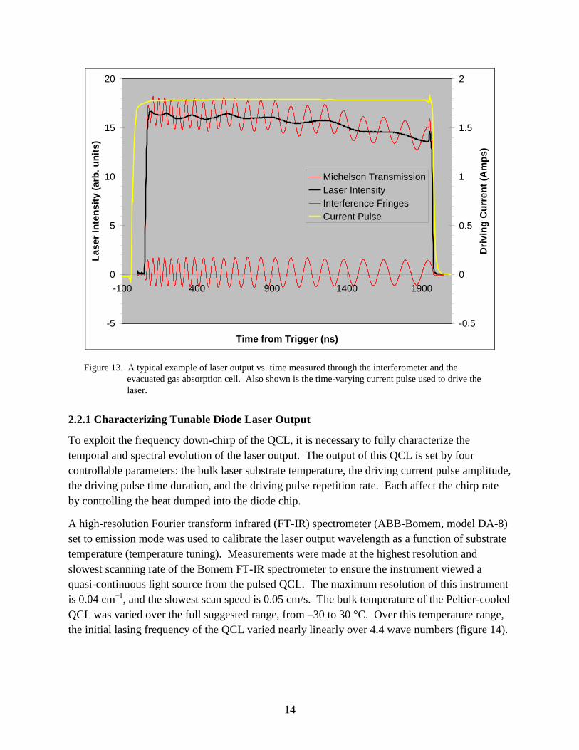
This report summarizes a 5-year effort at the U.S. Army Research Laboratory to study soot formation in diffusion flames. The
work described begins with experimental and modeling studies of atmospheric pressure ethylene (C2H4)/air (N2-O2) flames to
which metaxylene (C8H10) is added on the fuel side. Several laser-based diagnostic methods are discussed, including an
extensive effort to measure acetylene gas in flames using a quantum cascade laser. The report also describes efforts to
construct an elevated pressure-opposed flow burner and presents data on soot formation in ethylene/air flames in this burner to
a total pressure of ~3 bar. During the course of this work, new experimental techniques of high-speed digital temperature and
pressure mapping were developed. These techniques, described here in detail, became the focus of the latter part of the
research. They are also applied to flame analysis and explosion measurement as a way of illustrating the ability to measure
pressure and temperature during dynamic events. The report finishes with a discussion of unresolved or incomplete questions
and tasks, and a list of publications. 15. SUBJECT TERMS
Figure 1. A schematic of the opposed flow burner showing gas flow and flame location. ............2
Figure 2. A photograph of an ethylene/air-opposed jet flame showing the separation of sooting and combustion regions.................................................................................................3
Figure 3. A photograph of an ethylene/air flame within the burner chamber. ................................3
Figure 4. A schematic of the experimental apparatus, including some optical diagnostics. ..........4
Figure 5. Photo of elevated pressure rig in opposed flow configuration. .......................................5
Figure 6. Schematic of elevated pressure rig. .................................................................................5
Figure 7. The Collison-type atomizer. ............................................................................................6
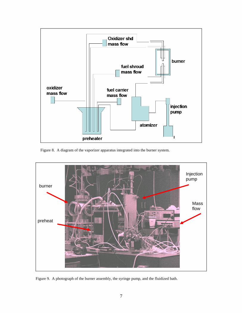
Figure 8. A diagram of the vaporizer apparatus integrated into the burner system. .......................7
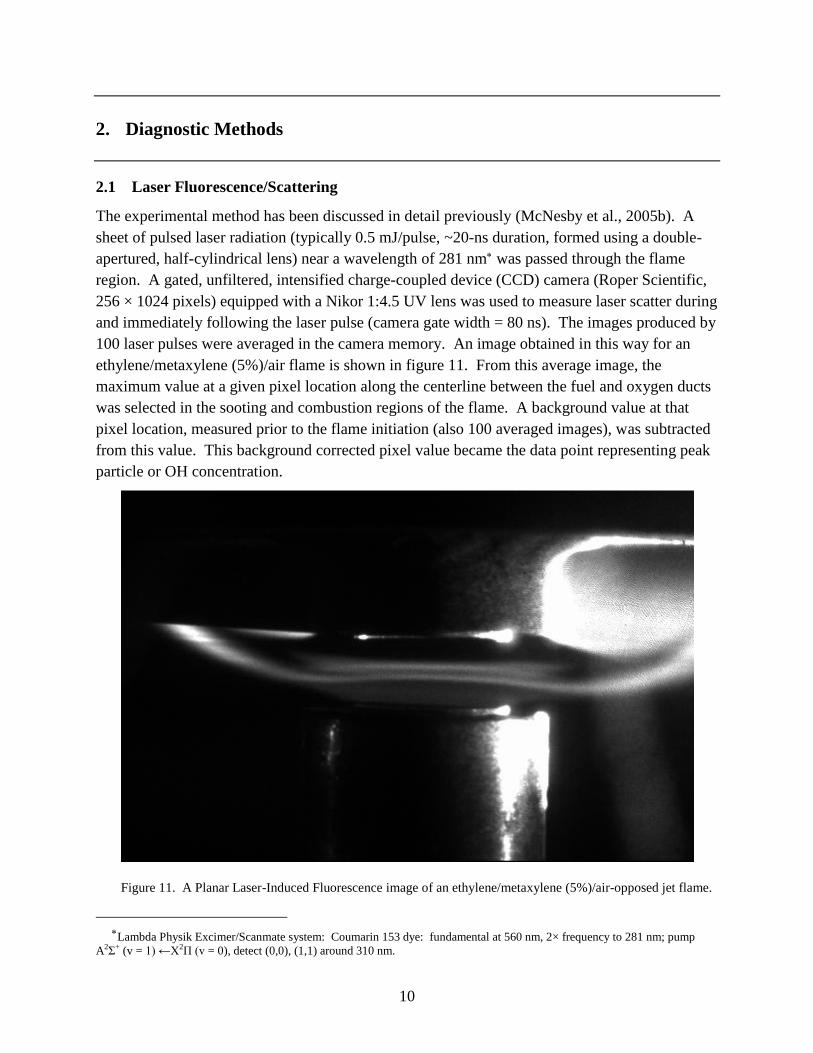
Figure 9. A photograph of the burner assembly, the syringe pump, and the fluidized bath. ..........7
Figure 10. The explosives test bed and assorted instrumentation composing the multipyrometry rig. ....................................................................................................................9
Figure 11. A Planar Laser-Induced Fluorescence image of an ethylene/metaxylene (5%)/air-opposed jet flame. ....................................................................................................................10
Figure 12. A schematic of the experimental setup for acetylene measurement by QCL. .............13
Figure 13. A typical example of laser output vs. time measured through the interferometer and the evacuated gas absorption cell. Also shown is the time-varying current pulse used to drive the laser. ......................................................................................................................14
Figure 14. Variation of initial lasing frequency with substrate temperature. ...............................15
Figure 15. The frequency down-chirp of the QCL output as a function of the amplitude of the driving current pulse. .........................................................................................................16
Figure 16. Acetylene transmission spectra converted to spectral absorbance and plotted against a calibrated frequency scale. ........................................................................................17
Figure 17. Integrated absorbance plotted against acetylene concentration and partial pressure. ...................................................................................................................................19
Figure 18. The Bayer CFA............................................................................................................22
Figure 19. The color imaging processing pipeline. A generic outline of steps that must be taken to transform light collected by a lens to reproduce a full-color image suitable for viewing. ....................................................................................................................................22
Figure 20. A Bayer CFA pattern with a (3×3) kernel used to calculate the mean values of the RGB channels at pixel (3,3). ....................................................................................................23
Figure 21. White balance is performed to correct for the spectral distribution of the light source. The intensity has been normalized at 575 nm. ...........................................................24
Figure 22. The analytical calibration curve (blue curve) and measured data from a blackbody source (red triangles)................................................................................................................24
vi
Figure 23. A power law gamma correction relating the voltage from the sensor (Vin) and the voltage out or pixel value (Vout). ......................................................................................26
Figure 24. Spectral transmittance of the filters that comprise the CFA. .......................................27
Figure 25. Ratio of the green to red channel in the temperature range expected for detonation products. ...................................................................................................................................28
Figure 26. Surface temperature maps of exploding spheres of a nitramine-based high explosive. .................................................................................................................................31
Figure 27. Predicted velocity and temperature profiles for the opposed jet burner using Unicorn and Chemkin Pro, ethylene/air flame, Wang-Colket mechanism. .............................33
Figure 28. A comparison of calculated acetylene profiles in the opposed jet ethylene/air flame (calculations are also shown using the Wang-Frenklach mechanism [Wang and Frenklach, 1997]). ....................................................................................................................33
Figure 29. Photographs of the opposed jet ethylene/air flame with increasing amounts of metaxylene added to the fuel gas. ............................................................................................34
Figure 30. Peak values of fluorescence/light scattering vs. fraction of metaxylene in fuel gas based on several series of measurements in the opposed jet burner, measured prior to rebuild of vaporizer apparatus. ................................................................................................35
Figure 31. Flame simulations using UNICORN (Katta et al., 2006), that predict increases in C6H6 (benzene) but modest changes in OH, with addition of metaxylene to the fuel side of ethylene/air flames. ..............................................................................................................36
Figure 32. (a) An example of a raw trace of centerline fluorescence intensity vs. height above fuel duct for neat (0%) and 4% fuel side addition of metaxylene to ethylene/air diffusion flames after vaporizer rebuild. (b) OH fluorescence intensity (centerline) for 0%–5% addition of metaxylene to the fuel side of the atmospheric pressure ethylene/air opposed jet flame. ....................................................................................................................37
Figure 33. Change in PAH fluorescence/light scattering along the centerline of the burner for ethylene/air opposed flow flames, with metaxylene added to the fuel side after the atomizer was rebuilt. ................................................................................................................38
Figure 34. A reconstruction of the acetylene concentration (not temperature corrected) measured in absorption in an acetylene-air flame supported by a glass blower’s torch. Concentration values are in arbitrary units. .............................................................................39
Figure 35. Measured acetylene absorption through the flame region of an ethylene/air opposed flow flame to which acetylene is added on the fuel side. ..........................................40
Figure 36. A photograph of the ethylene-air candle-like diffusion flame supported on a glass blower’s torch. .........................................................................................................................41
Figure 37. Temperature maps using the imaging pyrometer technique for acetylene-air and ethylene-air diffusion flames. ..................................................................................................41
Figure 38. The wavelength-resolved emission from three ethylene air flames ranging from a candle-like diffusion flame to a coflowing diffusion flame to an opposed jet flame. .............42
Figure 39. The imaging pyrometer technique applied to an opposed jet ethylene/air flame. .......43
Figure 40. Neat ethylene/air-opposed flow flame results from McNesby et al. (2005b). ............44
vii
Figure 41. Modeling predictions conducted at 1 atm with Cantera. .............................................45
Figure 42. Modeling predictions conducted at 2.04 atm (30 psi) with Cantera............................45
Figure 43. Modeling predictions conducted at 5 atm with Cantera. .............................................46
Figure 44. The modified high-pressure strand burner enclosure used to house the elevated pressure-opposed jet burner. ....................................................................................................47
Figure 45. The elevated pressure burner assembly in co-flow mode on the test bed. One of the sapphire window ports has been removed. ........................................................................47
Figure 46. The elevated pressure burner assembly in co-flow mode on the test bed, with the sapphire window port removed. The fuel/air duct is visible within the chamber interior. .....48
Figure 47. The elevated pressure-opposed flow rig, showing the gated intensified camera (CCD) used to image planar LIF. ............................................................................................49
Figure 48. A side view of the elevated pressure-opposed flow rig on the test stand. The IR cutoff filter is shown in front of the sapphire window through which flame images are recorded for temperature measurement. ..................................................................................49
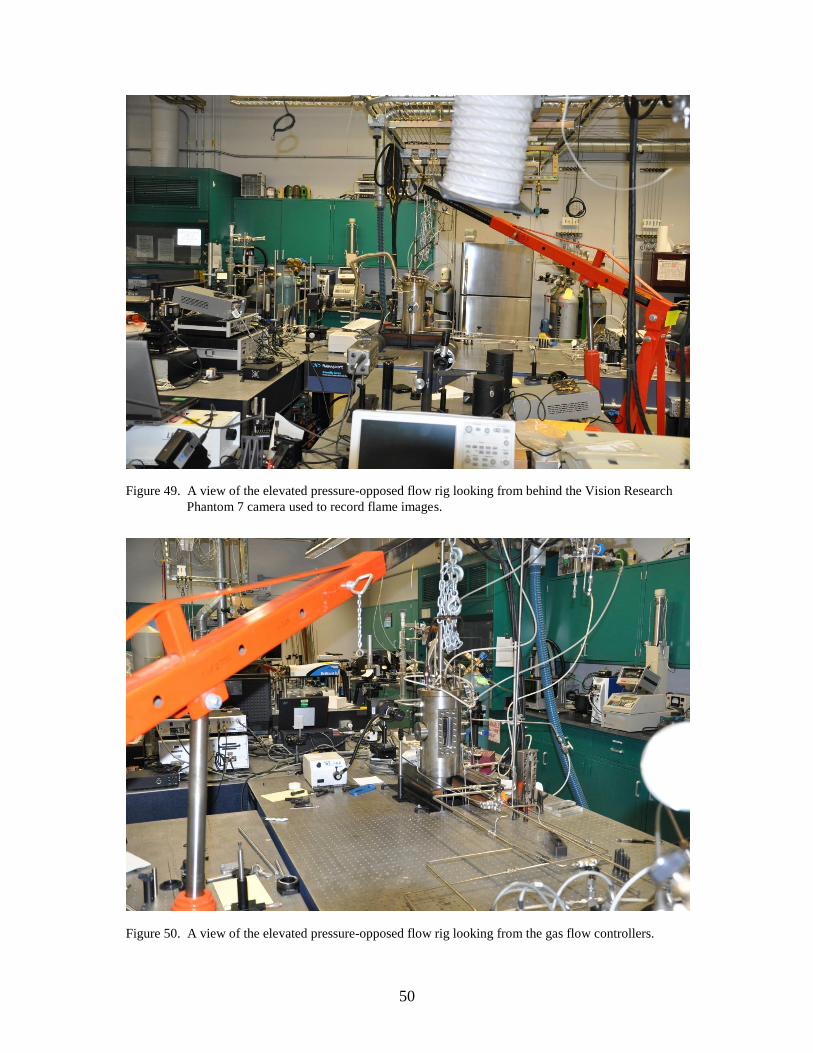
Figure 49. A view of the elevated pressure-opposed flow rig looking from behind the Vision Research Phantom 7 camera used to record flame images. .....................................................50
Figure 50. A view of the elevated pressure-opposed flow rig looking from the gas flow controllers. ...............................................................................................................................50
Figure 51. A view of the elevated pressure-opposed flow rig. The opposing fuel and air ducts are visible within the burner enclosure interior. .............................................................51
Figure 52. Raw images of elevated pressure-opposed flow flames at constant molar flow rate taken using a high-speed camera. It was necessary to adjust the camera exposure for each run to avoid saturating the camera chip. ..................................................................................52
Figure 53. Peak centerline temperatures (K) for elevated pressure ethylene/air flames at constant molar flow and at constant strain. Elevated pressure-opposed flow burner, ethylene/air flame. Temperatures are calculated using images in figures 51 and 52. ............53
Figure 54. Peak intensity per pixel per microsecond exposure along the burner centerline for the red pixel matrices (570–700 nm) from images of elevated pressure-opposed flow ethylene/air flames. ..................................................................................................................53
Figure 55. Raw images of elevated pressure-opposed flow flames at constant strain rate taken using a high-speed camera. It was necessary to adjust the camera exposure for each run to avoid saturating the camera chip. ..................................................................................54
Figure 56. (Top) Intensity ratio vs. temperature comparison of Wien’s approximation and an exact solution. (Bottom) Error vs. intensity ratio between Wien’s approximation and an exact solution. ..........................................................................................................................57
Figure 57. Wavelength of peak specific intensity vs. temperature. ..............................................59
Figure 58. Schematic of the three-color integrating pyrometer rig. .............................................60
Figure 59. Comparison of solar radiation both outside the atmosphere and at sea level with emission from an ideal blackbody at 5900 K. The baselines have been shifted for clarity. ...62
viii
Figure 60. (Top) Schematic of the single-axis two-color imaging pyrometer showing the lens and beam splitter arrangement. (Bottom) Band pass of each camera superimposed upon the emission from a blackbody near 2000 K. ..........................................................................63
Figure 61. (Top) Schematic of the full-color imaging pyrometer showing the Bayer-type mask in front of the sensor chip. (Bottom) Pixel calibration example from a Vision Research Phantom 5.1 camera. ................................................................................................65
Figure 62. (Top) Wavelength-resolved emission for three types of ethylene/air flames. (Bottom) Detail of emission from the OPPDIF flame showing emission bands due to CH and C2. ......................................................................................................................................66
Figure 63. Raw three-color integrating pyrometer data for a 227-g spherical C-4 charge, 19.0-cm standoff. .....................................................................................................................67
Figure 64. (Left) Calculated three-color integrating pyrometer temperatures for a 227-g spherical C-4 charge at 19.0-cm standoff. (Right) Average temperature profile from the three calculated temperatures. ..................................................................................................68
Figure 65. Average three-color integrating pyrometer calculated temperature profile for a 227-g spherical C-4 charge at 19.0-cm standoff. .....................................................................69
Figure 66. Average temperature profile calculated from all charges at a specified standoff distance with the three-color integrating pyrometer. ...............................................................70
Figure 67. Average three-color integrating pyrometer calculated temperature profile for the three 454-g spherical C-4 charges at 44.4-cm standoff distance, compared to the average temperature profile from the 227-g charges at that standoff....................................................71
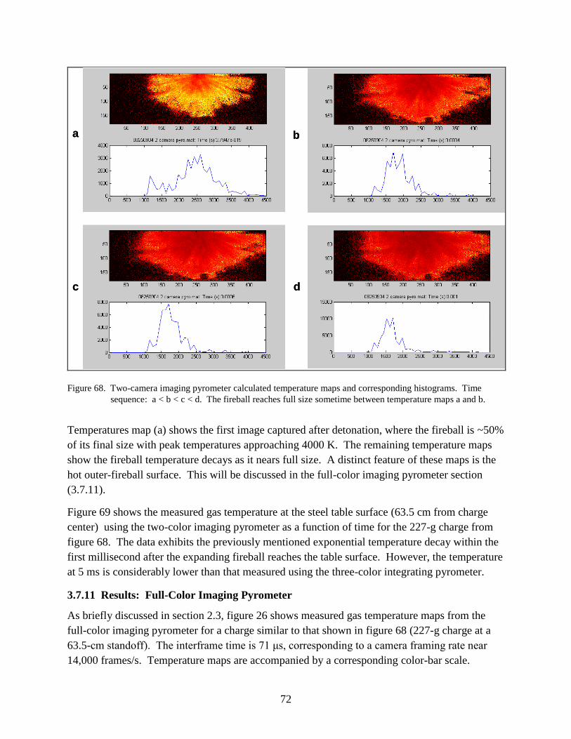
Figure 68. Two-camera imaging pyrometer calculated temperature maps and corresponding histograms. Time sequence: a < b < c < d. The fireball reaches full size sometime between temperature maps a and b. .........................................................................................72
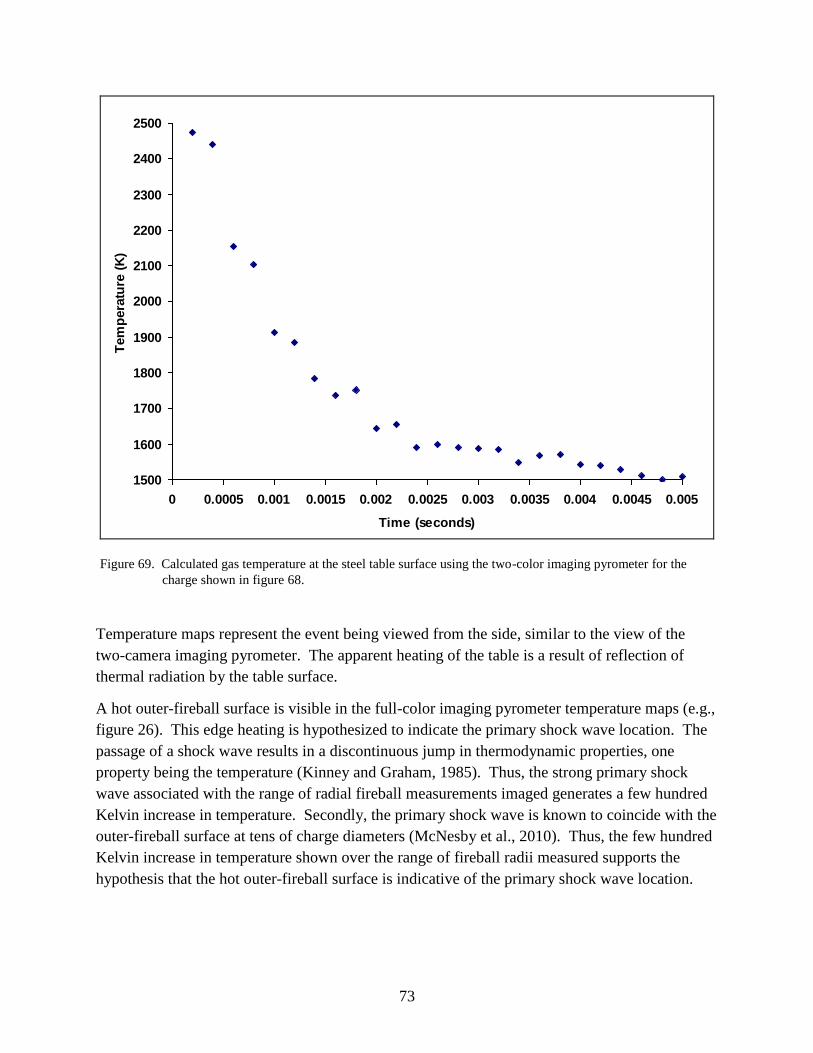
Figure 69. Calculated gas temperature at the steel table surface using the two-color imaging pyrometer for the charge shown in figure 68. ..........................................................................73
Figure 70. Full-color pyrometer extracted gas temperatures at the steel table surface vs. time for 227-g C-4 charges at the five standoff distances................................................................74
Figure 71. Gas temperatures at the steel table surface for the 227- and 454-g charges at a standoff of 44.4 cm. .................................................................................................................75
Figure 72. Average optically measured peak shock wave pressure at the steel table surface for the 227-g C-4 charges at the five standoff distances measured. ........................................76
Figure 73. Emission spectrum for the charge shown in figure 15 (227 g of C-4 at 63.5-cm standoff). The feature (doublet) near 589 nm is from sodium (Na) emission. .......................77
Figure 74. Temperatures measured for a 227-g C-4 charge at 63.5-cm standoff using each pyrometry method. ...................................................................................................................78
ix
List of Tables
Table 1. Temperature dependence of the line strength of the P(23) absorption line of the (υ4+ υ5) compound bending vibration of C2H2.........................................................................20
x
Preface
This report summarizes a 5-year effort at the U.S. Army Research Laboratory (ARL) to study
soot formation in diffusion flames. The work described in what follows begins with
experimental and modeling studies of atmospheric pressure ethylene (C2H4)/air (N2-O2) flames
to which metaxylene (C8H10) is added on the fuel side. Several laser-based diagnostic methods
are discussed, including an extensive effort to measure acetylene gas in flames using a quantum
cascade laser. The report also describes efforts to construct an elevated pressure-opposed flow
burner and presents data on soot formation in ethylene/air flames in this burner to a total pressure
of ~3 bar. During the course of this work, new experimental techniques of high-speed digital
temperature and pressure mapping were developed. These techniques, described here in detail,
became the focus of the latter part of the research. They are also applied to flame analysis and
explosion measurement as a way of illustrating the ability to measure pressure and temperature
during dynamic events. The report finishes with a discussion of unresolved or incomplete
questions and tasks, and a list of publications.
Overall, ARL’s effort on this overall task was moderately successful. The elevated pressure-
opposed flow burner required 3 years to become operational (this includes an 8-month safety
stand down at the laboratory). Several planned experiments at elevated pressure have yet to be
completed. A major accomplishment of this study is the establishment at ARL of a working
elevated pressure-opposed flow burner equipped for analysis using active laser-based methods.
The development of several new high-speed pyrometry measurements during this program
should prove valuable in the long term to the combustion and explosion community. We believe
this aspect of the work will advance the application of digital imaging to measurement of
physical parameters of flames and explosions.
xi
Acknowledgments
The authors wish to thank Dr. Mel Roquemore and Prof. Tom Litzinger for the helpful, honest
assessments of this work, and Dr. Eric Bukowski for a detailed review of this manuscript.
The authors would also like to thank the Strategic Environmental Research and Development
Program for funding the developmental work on the elevated pressure burner, the quantum
cascade laser for acetylene measurement, and the two-color and full-color pyrometer rigs. The
Department of Homeland Security provided support for some of the exterior testing. Support is
also acknowledged from the Defense Threat Reduction Agency. This research was supported in
part by an appointment to the U.S. Army Research Laboratory (ARL) Postdoctoral Fellowship
Program administered by the Oak Ridge Associated Universities and National Research Council
through a contract with ARL. Support was also provided by a grant from the National Research
Council.
xii
INTENTIONALLY LEFT BLANK.
1
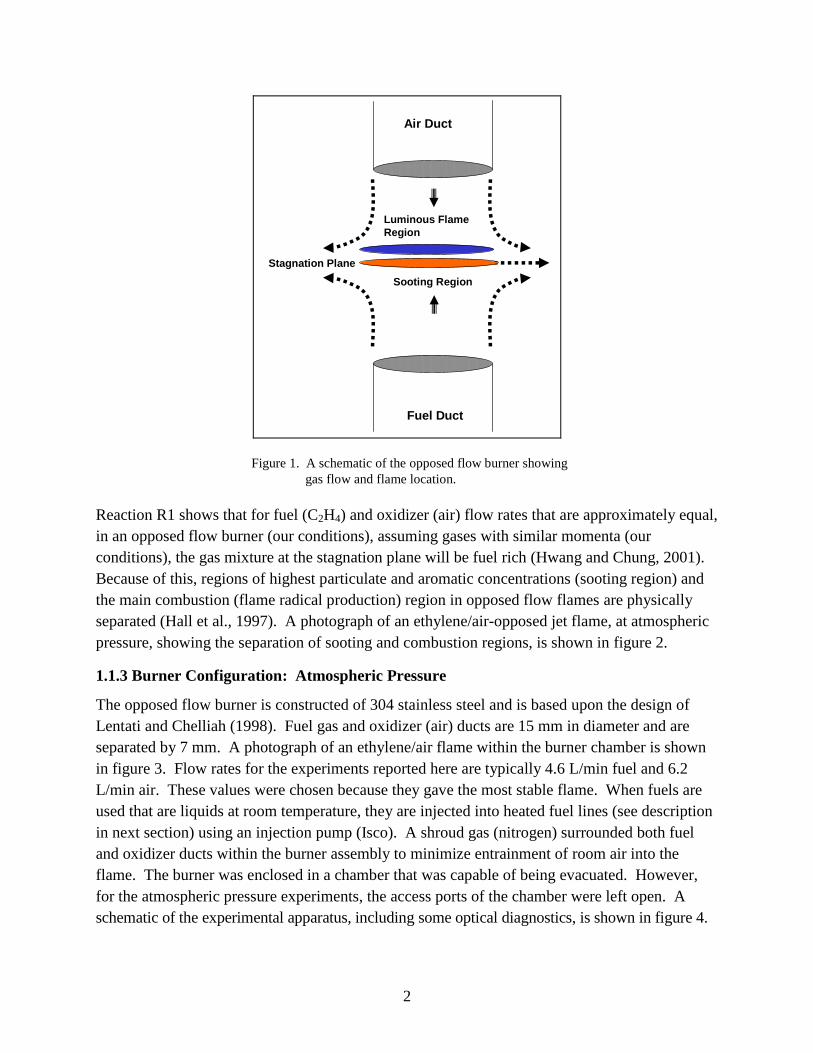
1. Testing Rigs
1.1 Opposed Jet Diffusion Flame
1.1.1 Introduction
Previous Strategic Environmental Research and Development Program (SERDP)-related studies
using the U.S. Army Research Laboratory (ARL) opposed jet diffusion flame burner have
concentrated on soot formation in atmospheric pressure ethylene/air flames (McNesby et al.,
2005b). For the current program investigating soot formation, this burner has been modified to
operate at fuel side temperatures up to 250° centigrade, enabling the use of many fuels that are
liquids at room temperature. Opposed jet diffusion ethylene/air flames have also been
investigated at elevated pressure (5-bar total pressure) using an opposed jet burner flame
apparatus constructed at ARL. The flames supported in these burners are probed using several
types of optical diagnostics, including laser-induced fluorescence (LIF), laser scattering, tunable
diode laser absorption spectroscopy (TDLAS), and multicolor pyrometry. The experimental
apparati, methods, and techniques developed for the ARL effort are described in what follows.
Experiments using our liquid-fuels-capable opposed jet burner have focused on ethylene/air
flames to which metaxylene (C8H10) has been added to the fuel side at levels up to 20% by gas
volume, by the methods described in section 1.1.4. For each flame system to which metaxylene
is added, the ethylene gas flow is reduced to maintain equal carbon content in the gas flow
entering the flame zone. When added in this manner, the visual effect of adding metaxylene to
the fuel gas is to increase the luminosity of the sooting region of the flame (figure 29) while
having limited effect on the luminous “blue” flame region. The lower “yellow” region of the
flame may contain soot particles and aromatics. For this reason, LIF from this region is referred
to as poly-aromatic hydrocarbon (PAH) fluorescence/light scattering.
Figure 29. Photographs of the opposed jet ethylene/air flame with increasing amounts of metaxylene
added to the fuel gas.
0%
5%
10%
15%
20%
35
Figure 30 shows initial results of measurements of PAH fluorescence/light scattering and of OH
fluorescence vs. fraction of metaxylene in fuel gas based on several series of measurements in
the opposed jet burner. A surprising result was that the increase in PAH fluorescence/light
scattering from this “sooting” region was accompanied by an initial large decrease in OH
fluorescence. Modeling results using the SERDP mechanism and the mechanism of Violi predict
the increase in the “sooting” region but predict little change in OH (figure 31). A close
examination of figure 30 shows that the largest decrease in measured OH occurs when going
from the neat flame (0% metaxylene) to a 4% metaxylene loading of the fuel gas (ethylene). To
double-check these initial results, the vaporizer apparatus was rebuilt and experiments rerun,
varying carrier gas flow rates to ensure that all metaxylene injected into the atomizer was being
entrained in the fuel gas.
Figure 30. Peak values of fluorescence/light scattering vs. fraction of metaxylene in fuel gas
based on several series of measurements in the opposed jet burner, measured prior to
rebuild of vaporizer apparatus.
0
5
10
15
20
25
30
0 5 10 15 20 25
Percent C8H10
Peak F
luo
rescen
ce
OH
PAH
5% metaxylene
36
Figure 31. Flame simulations using UNICORN (Katta et al., 2006), that predict increases in C6H6
(benzene) but modest changes in OH, with addition of metaxylene to the fuel side of
ethylene/air flames.
Figures 32 and 33 show results of a careful remeasurement of PAH fluorescence/light scattering
and OH fluorescence vs. fraction of metaxylene in fuel gas (holding total C constant), focusing
on the region (0%–5% metaxylene) of largest decrease in OH from initial experiments. Figure
32 shows that the initial decrease in OH with the addition of metaxylene was not repeatable, after
the atomizer was rebuilt. Figure 33 shows the increase in light scattering/soot formation for this
same range of metaxylene addition after the rebuild.
The new results are in agreement with predictions based upon UNICORN for the opposed flow
ethylene/air flames to which metaxylene is added on the fuel side. The nonrepeatability of the
initial results serves to emphasize the care with which the vaporizer system must be maintained.
37
Figure 32. (a) An example of a raw trace of centerline fluorescence intensity vs. height above fuel duct for
neat (0%) and 4% fuel side addition of metaxylene to ethylene/air diffusion flames after
vaporizer rebuild. (b) OH fluorescence intensity (centerline) for 0%–5% addition of
metaxylene to the fuel side of the atmospheric pressure ethylene/air opposed jet flame.
(a)
(b)
0
100
200
300
400
500
600
700
800
900
1000
0 1 2 3 4 5 6
% meta-xylene
OH
Flu
ore
scen
ce
0
100000
200000
300000
400000
500000
600000
700000
0 1 2 3 4 5 6 7
Height Above Fuel Duct (mm)
Flu
orescen
ce In
ten
sit
y (
arb
. u
nit
s)
neat
4 pct
38
Figure 33. Change in PAH fluorescence/light scattering along the centerline of the burner for
ethylene/air opposed flow flames, with metaxylene added to the fuel side after the
atomizer was rebuilt.
3.3 Tunable Diode Laser Absorption Spectroscopy
Acetylene measurements in flames have been measured using methods described in section 2.2.
Work describing the application of this technique to characterization of an acetylene-air diffusion
flame has been published in Applied Optics (Quine and McNesby, 2009). A reconstruction of
the acetylene concentration (not temperature corrected) measured in an acetylene-air flame
supported by a glass blower’s torch is shown in figure 34. This technique has been extended to
measurements in the opposed flow burner. Figure 35 shows a measurement of acetylene
absorption through the flame region, by the method described in section 2.2, of an ethylene/air-
opposed flow flame to which acetylene is added on the fuel side. The feature labeled as the P23
line of acetylene demonstrates the capability of the technique to measure acetylene produced in
the ethylene/air-opposed jet flame. As pointed out in section 2.2, quantitative measurement of
acetylene concentrations in the flame using IR absorption techniques requires knowledge of
temperature.
0
100
200
300
400
500
600
700
800
0 1 2 3 4 5 6
% meta-xylene
PA
H F
luo
rescen
ce
39
Figure 34. A reconstruction of the acetylene concentration (not temperature corrected)
measured in absorption in an acetylene-air flame supported by a glass blower’s
torch. Concentration values are in arbitrary units.
40
Figure 35. Measured acetylene absorption through the flame region of an ethylene/air opposed flow flame to
which acetylene is added on the fuel side.
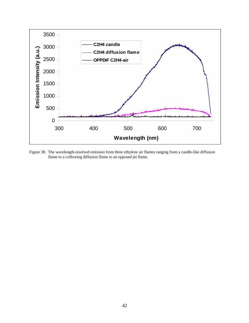
3.4 Imaging Pyrometry
The imaging pyrometer described in section 2.3 was initially tested on the diffusion flame
described in the previous section for acetylene measurement. A photograph of this flame
(ethylene-air diffusion) is shown in figure 36. Temperature maps using the imaging pyrometer
technique for acetylene-air and ethylene-air diffusion flames are shown in figure 37. (The
imaging pyrometer is best suited to measure temperatures of particle laden, i.e., sooting, flames.)
For flames that exhibit minimal graybody emitters or have significant discrete spectral emission,
the technique may report inaccurate temperatures. As an example, figure 38 shows the
wavelength-resolved emission from three ethylene/air flames ranging from a candle-like
diffusion flame to a coflowing diffusion flame to an opposed jet flame. Each flame shows
differing contributions to total emission from discrete emission. Therefore, when using this
technique, we believe it is mandatory that a measurement of wavelength-resolved emission also
be recorded. Figure 39 shows the imaging pyrometer technique applied to an opposed jet
ethylene/air flame. The pyrometer yields reasonable temperatures in the sooting region of the
flame, but the blue-green emission from CH and C2 causes the pyrometer to report inaccurate
temperatures in the combustion region of the flame.
Effect of Acetylene Doping of Ethylene Flame Opposed Flow Flame
-0.02
0.03
0.08
0.13
0.18
0.23
0 1 2 3 4 5 6
Time of Scan (us)
Ab
so
rba
nce
(A
U)
Ethylene Flame
Doped 10% Acetylene
LDoped 20% Acetylene
Ethylene Acet Off
Background
Acety
lene P
24
1273.2
6 c
m-1
Acety
lene P
22
1277.7
6 c
m-1
Acety
lene
P23
1275.5
1 c
m-1
Wate
r
Wate
r
Wate
r
Wate
r
Wate
r
Wate
r
41
Figure 36. A photograph of the ethylene-air candle-like
diffusion flame supported on a glass blower’s
torch.
Figure 37. Temperature maps using the imaging pyrometer technique for acetylene-air and ethylene-air diffusion
flames.
•Flame Temperature of Acetylene diffusion flame ~1830 °C•Flame Temperature of Ethylene diffusion flame ~1760 °C
•Flame Temperature of Acetylene diffusion flame ~1830 °C•Flame Temperature of Ethylene diffusion flame ~1760 °C
42
Figure 38. The wavelength-resolved emission from three ethylene air flames ranging from a candle-like diffusion flame to a coflowing diffusion flame to an opposed jet flame.
0
500
1000
1500
2000
2500
3000
3500
300 400 500 600 700
Wavelength (nm)
Em
issi
on
In
ten
sity
(a.
u.)
C2H4 candle
C2H4 diffusion flame
OPPDIF C2H4-air
43
Figure 39. The imaging pyrometer technique applied to an opposed jet ethylene/air flame.
3.5 Applications to Elevated Pressure Flames: Modeling
Modeling was conducted using the Appel, Bockhorn, and Frenklach (ABF) mechanism, which
contains 101 species, 544 reactions, and associated thermodynamic and transport files (Appel et
al., 2000). The ABF mechanism has been validated with ethane, ethylene, and acetylene fuels
and predicts the major, minor, and aromatic species up to pyrene. The ABF mechanism was
executed with Cantera, which is an open-source, multiplatform software code used to study
combustion behavior using the 1-D counter-flow flame configuration. Initial grid spacing
between inlets was evenly set to 0.0, 0.2, 0.4, 0.6, 0.8, 1.0 cm for 1-atm calculations and then
modified to 0.0, 0.1, 0.2, 0.3, 0.4, 0.5, 0.6, 0.8, 1.0 cm for simulations at elevated pressures.
44
Once the Newton iteration successfully converged, grid refinement was enabled and new grid
points were inserted to proceed with the calculation. Final grid count included 172, 161, and 172
points for 1, 2.04 (30 psi), and 5 atm, respectively. The computational time, using a Pentium
Dual-Core T4400 processor with a 64-bit operating system, for convergence to occur was
~180 s. Initial conditions of the model simulations were set to the following: ethylene as fuel;
air as oxidizer; fuel/oxidizer inlet temperature of 300 K; duct separation of 1 cm; initial pressure
of 1, 2.04 (30 psi), and 5 atm for each case; and mass flux of fuel and oxidizer set to 0.47 and
0.65 kg/m2/s, respectively.
Initial modeling results conducted at 1-atm pressure were compared to experimental and
modeling results from McNesby et al. (2005b) (figure 40). The experimental study consisted of
using an opposed flow burner with ethylene as fuel and air as oxidizer. Burner dimensions
consisted of a 1-cm inlet separation and 1.5-cm duct diameter. Flow rates of the fuel and
oxidizer were 4.6 and 6.2 L/min, respectively. The computational study consisted of using the
ABF mechanism with a modification to include ethanol addition. The mechanism was executed
using OPPDIF flow code, based on the Chemkin database. The modified chemical mechanism
includes 156 species and 659 reactions. When a Pentium 4–based computer was used,
convergence required 100 min. Figure 40 shows the experimental and modeling results from
the neat ethylene/air-opposed flow flames. For the ABF mechanism, A1 and A4 represent
benzene and pyrene, respectively.
Figure 40. Neat ethylene/air-opposed flow flame results from McNesby et al. (2005b).
45
The modeling results using Cantera are shown in figures 41–43. The results from the Cantera
calculations, as shown in figure 41, agree with the results from the Chemkin calculations, shown
in figure 40. Both Chemkin and Cantera simulations capture the formation of benzene near the
fuel inlet fuel-rich conditions and the formation of OH as the fuel diffuses into the oxidizer
stream. To explore the effects of pressure on the formation of species using Cantera,
calculations were also executed at 2.04 atm (2 bar) and 5 atm pressure (5 bar). Figure 42 shows
the calculations at 2.04 atm. As the pressure is doubled from 1 atm, the production of benzene
increases as the production of C3H3 decreases. In addition, an increase in temperature is also
observed as the pressure increases. These observations are more predominant as the pressure is
increased to 5 atm, as shown in figure 43.
Figure 41. Modeling predictions conducted at 1 atm with Cantera.
Figure 42. Modeling predictions conducted at 2.04 atm (30 psi) with Cantera.
0
500
1000
1500
2000
2500
0
0.1
0.2
0.3
0.4
0.5
0.6
0.7
0.8
0.9
1
0 0.2 0.4 0.6 0.8 1
Tem
pe
ratu
re (K
)
Mo
le F
ract
ion
Distance From Fuel Duct (cm)
OH X 50
C3H3 X 5000
C6H6 X 1000
Temperature
0
500
1000
1500
2000
2500
0
0.1
0.2
0.3
0.4
0.5
0.6
0.7
0.8
0.9
1
0 0.2 0.4 0.6 0.8 1
Tem
pe
ratu
re (K
)
Mo
le F
ract
ion
Distance From Fuel Duct (cm)
OH X 50
C3H3 X 5000
C6H6 X 1000
Temperature
46
Figure 43. Modeling predictions conducted at 5 atm with Cantera.
3.6 Applications to Elevated Pressure Flames: Experiments
The elevated pressure burner could be operated in co-flow or opposed flow configuration. In
co-flow mode (results not reported here), the upper duct assembly was removed and replaced
with a blank-off plate. In this mode, fuel gas was flowed through the central, lower duct, and
oxidizer (air) was flowed through the shroud duct that surrounded the fuel duct. Operation in
this mode has been verified to 4 bar. Figures 44–46 show the elevated pressure burner in
co-flow mode mounted on the test stand.
For opposed flow mode, the blank-off flange at the top of the elevated pressure burner was
replaced by a top assembly that contained fitment to allow for introduction of cooling water,
oxidizer and shroud gases, and supplemental exhaust gas ports. Figures 47–51 show the elevated
pressure burner in opposed flow mode mounted on the test stand. Several pieces of diagnostic
equipment used to measure flame temperatures and radical concentrations are also shown in
these images.
In constant molar flow mode, as the pressure is increased, the densities of the fuel and oxidizer
gasses change. For experiments reported here, we have run the burner in constant molar flow
mode and in constant strain mode. In constant molar flow mode, the flow rate set at the flow
controllers is kept constant. For the opposed flow burner configuration used here (1.4-cm
diameter, 0.6-cm duct separation), the flow rate used in constant molar flow mode was 2.7 L/min
air and 4 L/min ethylene. For a stagnation plane located midway between the burner ducts, this
corresponds to a global oxidizer strain rate of 97 s–1
at a total pressure of 1 bar.
0
500
1000
1500
2000
2500
0
0.1
0.2
0.3
0.4
0.5
0.6
0.7
0.8
0.9
1
0 0.2 0.4 0.6 0.8 1
Tem
pe
ratu
re (K
)
Mo
le F
ract
ion
Distance From Fuel Duct (cm)
OH X 50
C3H3 X 5000
C6H6 X 1000
Temperature
47
Figure 44. The modified high-pressure strand burner enclosure used to
house the elevated pressure-opposed jet burner.
Figure 45. The elevated pressure burner assembly in co-flow mode on the test bed. One of the
sapphire window ports has been removed.
48
Figure 46. The elevated pressure burner assembly in co-flow mode on the
test bed, with the sapphire window port removed. The fuel/air
duct is visible within the chamber interior.
49
Figure 47. The elevated pressure-opposed flow rig, showing the gated intensified camera (CCD) used
to image planar LIF.
Figure 48. A side view of the elevated pressure-opposed flow rig on the test stand. The IR cutoff filter
is shown in front of the sapphire window through which flame images are recorded for
temperature measurement.
50
Figure 49. A view of the elevated pressure-opposed flow rig looking from behind the Vision Research
Phantom 7 camera used to record flame images.
Figure 50. A view of the elevated pressure-opposed flow rig looking from the gas flow controllers.
51
Figure 51. A view of the elevated pressure-opposed flow rig. The opposing fuel and air ducts are visible
within the burner enclosure interior.
In constant molar flow mode, as pressure is increased, density decreases, so strain rate also
decreases. Visually, as pressure increases, the flame changes from a mixture of blue and orange
near atmospheric pressure to a bright orange at pressures >2 bar. Figure 52 shows a series of
photographs of the constant molar flow flame from atmospheric pressure to above 2 bar total
pressure. These images are all taken with the red pixel matrix near 80% of saturation. Prior to
each image being taken, the exposure was adjusted so that none of the color pixels corresponding
to a point in the flame were at saturation. From these images, the gradual change from blue to
orange is evident. Figure 53 shows a plot of temperatures measured using imaging pyrometry as
described here. As the pressure is increased for the constant molar flow flames, the measured
temperature decreases. This is in disagreement with flame temperatures predicted using Cantera.
Figure 54 shows a plot of pixel intensity along the burner centerline for the red pixel matrix
(sensitivity 530 to 700 nm). Pixel values are reported in counts per microsecond of exposure to
account for variations in exposure time used when obtaining the original images. As pressure is
increased, the pixel value per microsecond exposure increases. As soot incandescence at flame
temperatures peaks in the red pixel matrix spectral region, we imply an approximate correlation
between the pixel intensity in this spectral region and soot volume fraction. The increase in soot
volume fraction with pressure is in agreement with increases in benzene (C6H6) with pressure as
predicted using Cantera.
52
Figure 52. Raw images of elevated pressure-opposed flow flames at constant molar flow rate taken using a
high-speed camera. It was necessary to adjust the camera exposure for each run to avoid
saturating the camera chip.
530 torr
5000 usec 6000 us
870 torr 968 torr
3000 usec
1000 usec
12 psi10 psi
2500 usec
15 psi
1000 usec
800 usec
20 psi
4 l/m ethylene2.7 l/m air
53
Figure 53. Peak centerline temperatures (K) for elevated pressure ethylene/air flames at constant molar flow and
at constant strain. Elevated pressure-opposed flow burner, ethylene/air flame. Temperatures are
calculated using images in figures 51 and 52.
Figure 54. Peak intensity per pixel per microsecond exposure along the burner centerline for the red pixel
matrices (570–700 nm) from images of elevated pressure-opposed flow ethylene/air flames.
0
500
1000
1500
2000
2500
3000
0.5 1 1.5 2 2.5 3
Pe
ak C
en
terl
ine
Te
mp
era
ture
(K
)
Pressure (Bar)
T (K) constant molar flow
T (K) constant strain
0
0.05
0.1
0.15
0.2
0.25
0.3
0.35
0.4
0.45
0 0.5 1 1.5 2 2.5 3
Inte
nsi
ty p
er
pix
el/
use
c (5
70
-70
0 n
m)
Pressure (Bar)
Constant molar flow
Constant strain
54
For constant strain mode, the flow rate of fuel and oxidizer gases was varied to account for
changes in gas density as pressure was increased. At atmospheric pressure, the initial flame was
based upon a flow rate of 2 L/min oxidizer and 2.9 L/min ethylene. At our burner configuration,
this resulted in a global oxidizer strain rate of 72 s–1
. To maintain this strain rate up to a total
pressure approaching 3 bar, the oxidizer flow rate was eventually raised to 5.4 L/min (with a
concurrent increase in fuel flow rates). Images of these flames measured using the same
methodology as for constant molar flow flames are shown in figure 55. As seen for constant
molar flow rate flames, the most notable visual change with increasing pressure was an increase
in luminosity as the flames changed from a mixture of blue and orange to bright orange.
Figure 53 shows the temperature decreasing with increasing pressure for the constant strain rate
flames. Figure 54 shows the 530- to 700-nm pixel intensity per microsecond exposure
increasing with pressure. At present, we have no explanation for the disagreement between
measured temperatures and those predicted using Cantera for either of the elevated pressure-
opposed flow flames reported here.
Figure 55. Raw images of elevated pressure-opposed flow flames at constant strain rate taken using a high-
speed camera. It was necessary to adjust the camera exposure for each run to avoid saturating
the camera chip.
450usec 750 us
25 psi 20 psi
3000 us
15 psi 10 psi
4000 us
1000 torr
3000 usec 4000 usec
749 torr 637 torr
4000 usec
Ethylene/air opposed flow flame – constant strain - Raw
55
3.7 Explosives Testing
An ideal explosive releases all of its energy instantaneously, allowing the explosive impulse at
any time or distance from charge center to be determined from pressure and temperature at time
zero (Kinney and Graham, 1985). However, as pointed out by Mader (2008), “All explosives are
non-ideal.” This means that chemical processes that influence explosive impulse and fireball
temperature can occur after explosive detonation at times later than predicted by standard
numerical codes (e.g., CHEETAH [Fried et al., 1998]). Traditional methods of measuring
explosive impulse and temperature are point measurements employing mechanical, piston-type,
piezo-based pressure transducers and thermocouples. Recently, measurements and calculations
performed at ARL suggest that the release of energy by nonideal explosives after initiation is
determined by product gas composition and temperature (McNesby et al., 2010). Therefore, to
accurately measure performance of nonideal explosives, it is necessary to map out pressure and
temperature fields immediately following initiation. Over the past several years, we have been
developing an optical approach that uses high-speed imaging to retrieve temperatures and
pressures from functioning explosives. Here, we summarize our efforts to date, using the high-
As mentioned previously, spectral intensity per unit wavelength Iλ can be determined through
Planck’s law (equation 13) (Planck, 1901). It states that spectral intensity is a function of
variables: wavelength λ, temperature T, and emissivity ελ, in addition to Planck’s constant h, the
speed of light in vacuum c, and the Boltzmann constant k.
1
125
2
kThc
e
hcI
.
(13)
In principle, temperature is determinable from a single intensity measurement at a known
wavelength. However, for a remote measurement made some distance away from the source, the
measured intensity will also be a function of geometry, light collection efficiency, instrument
transmission efficiency, and detector responsivity. Because of the practical difficulty in
accurately accounting for these complicating factors, two wavelength intensity measurements are
generally used to eliminate an arduous calibration (McNesby, 2005b). The temperature is thus
calculated from the ratio of intensities at two different wavelengths (equation 2). Upon
examination of equation 14, it is clear that an assumption must be made about emissivities ε1 and
ε2 to explicitly extract a temperature. The clear choice is to assume that the ratio of emissivities
is constant and unity. In other words, the fireball is assumed to behave as a graybody. Previous
work has shown this to be a valid assumption under a range of conditions (Levendis et al., 1992;
Panagiotou et al., 1996). However, for temperature measurements using emission from hot soot
particles, a wavelength-dependent emissivity correction is available (Murphy and Shaddix,
2004).
56
1
1
1
2
2
1
2
1
5
1
5
2
kThc
kThc
e
e
I
I
.
(14)
Wavelength-specific intensities measured by the photodiodes are modified by calibration
constant Ci to account for the previously disregarded variations in light collection geometry,
transmission efficiency, and detector responsivity. The calibration constant also compensates for
differing transmission widths of the band-pass filters, as long as the transmission width Δ λ is
small relative to λ 1 – λ 2. These factors are subsumed into a single calibration constant for each
photodiode. Thus, the ratio of any two measured intensities is expressed by equation 15. The
calibration constants C1,2 are determined through measurement of a calibration source at known
temperature.
2
1
2
1
2
1
IC
IC
S
S .
(15)
3.7.2 Wien’s Approximation
Equation 14 can be solved implicitly for temperature or explicitly by invoking Wien’s
approximation (equation 16) (Mehra and Rechenberg, 1982). Temperature may then be
expressed in terms of the known physical constants, wavelengths of interest, and detector signals
with calibration constants (equation 17).
kT
hckT
hc
ee 1 . (16)
12
1
2
21
lnln5ln
11
2
1
S
S
C
Ck
hcT . (17)
For wavelengths of interest used most often by us (i.e., 700, 820, and 900 nm), the maximum
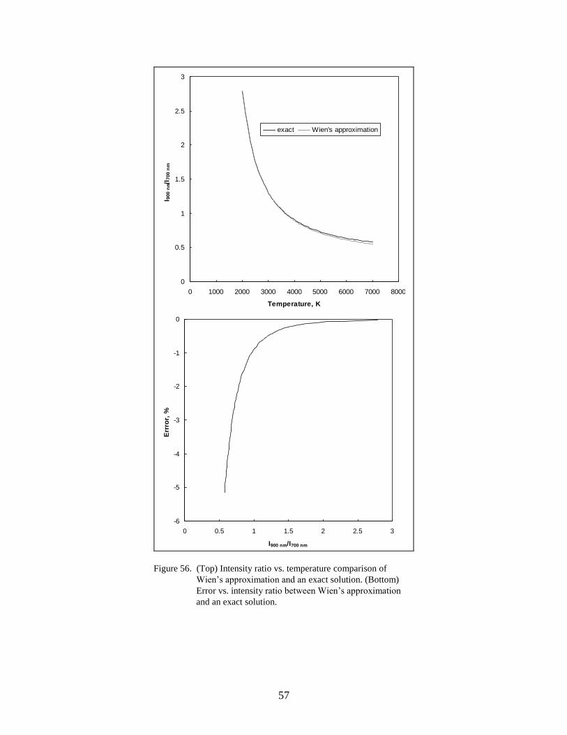
error introduced by Wien’s approximation compared to the exact solution is 5% at a temperature
of 6000 K. However, a 5% error at 6000 K is not insignificant. Figure 56 compares the intensity
ratio and resulting error as a function of temperature.
57
Figure 56. (Top) Intensity ratio vs. temperature comparison of
Wien’s approximation and an exact solution. (Bottom)
Error vs. intensity ratio between Wien’s approximation
and an exact solution.
0
0.5
1
1.5
2
2.5
3
0 1000 2000 3000 4000 5000 6000 7000 8000
Temperature, K
I 900
nm/I
700
nm
.
exact Wien's approximation
-6
-5
-4
-3
-2
-1
0
0 0.5 1 1.5 2 2.5 3
I900 nm/I700 nm
Err
ror,
%
.
58
It is possible to improve upon the calculated temperature of equation 17 and still obtain an
explicit solution. By finding an appropriate correction function for the measured intensity ratio,
21
,, 21 IIC f , the error introduced by Wien’s approximation is able to be compensated by
using equation 18.
12
2,1
21
21
lnln51
,,ln
11
2
1
S
S
cC
k
hcT
f
. (18)
The error in intensity ratio shown in figure 56 is fit with a power-law profile for temperatures
below 6000 K (equation 19). Constants a and b are dependent on the particular values of λ 1 and
λ 2 and were determined for all wavelength combinations through a linear least-squares
regression curve fit. A corrected-temperature profile is determined from equation 18 using the
correction function containing the superposition of the intensity ratio and error (equation 20).
When this method is used, the previous 300-K error at 6000 K is reduced to <4 K.
b
I
Ia
2
1
. (19)
1
2
1
2
1
b
fI
Ia
I
IC
. (20)
Spectral intensity measurements at multiple wavelengths serve as a verification of the integrating
pyrometer’s performance and validity of the assumptions outlined previously. In this case,
independent temperature calculations are made by choosing different signal pairs and checked
for agreement. The choice of wavelengths is governed by four main factors:
1. Intensity ratio at selected wavelength pairs should exhibit a strong temperature
dependence.
2. Individual intensity should be as large as possible to maximize the signal-to-noise ratio.
3. Emissivity should not vary greatly over the wavelength range of interest.
4. Any discrete emission from the system under measurement should not coincide with the
wavelengths chosen for temperature calculation.
For the three-color integrating pyrometer, a system with wavelengths of 700, 820, and 900 nm
was used. Figure 57 shows the wavelength of peak-specific intensity vs. temperature, with a
maximum in the near-IR region at temperatures of 2000–4000 K. Thus, temperatures may be
calculated as just described using any two of the three available optical-pyrometer signals.
59
Figure 57. Wavelength of peak specific intensity vs. temperature.
An equivalent temperature calculated by all three pairs adds confidence to the measurement and
decreases the likelihood that errors in the calibration or equipment malfunction will go
undiscovered.
3.7.3 Experimental
Experiments were conducted at an outdoor test range at APG. The test range consisted of a
rectangular concrete deck, 2100 m2, surrounded by barricaded control buildings. The
experimental apparatus consisted of an explosives test rig and optical diagnostics test rig
separated at the center of the concrete deck by ~12 m. The explosives test rig was centered on a
1.5 m2 table positioned 0.84 m above the concrete deck. The table surface was an 8.26-cm-thick
steel plate. Explosive charges were suspended over the table center by nylon string at standoff
distances of 12.7, 19.0, 31.8, 44.4, and 63.5 cm. Detonation was initiated by an RP-83 exploding
bridge-wire detonator. Diagnostic instrumentation was triggered by rupturing an illuminated
600-μm Si core optical fiber placed adjacent to the charge apex. Upon explosive initiation, a
trigger pulse was generated due to the abrupt loss of light transmission through the fiber.
0
200
400
600
800
1000
1200
1400
1600
0 2000 4000 6000 8000
Temperature, K
(I
max)
, n
m
.
60
The multi-imaging rig consists of four separate instruments: a three-color integrating pyrometer,
a two-camera imaging pyrometer, a full-color single-camera pyrometer (Densmore et al., 2011),
and a wavelength-resolved spectrograph (300–800 nm). Each pyrometer in the imaging rig
operates on the same scientific principle: determining temperature from spectral emission
intensity. The rig was enclosed in 1- × 1- × 2-m-tall armored enclosure (2.54-cm-thick steel)
with an ~30 cm2 viewing port positioned 1.22 m off the concrete deck. The viewing port was
uncovered to prevent the need to calibrate the pyrometers through window material and also
because there was no anticipated fragment danger from the uncased C-4 charges. A diagram of
the full test rig setup is shown below in figure 10.
3.7.4 Three-Color Integrating Pyrometer
Figure 58 shows a schematic of the three-color integrating optical pyrometer. This pyrometer rig
has the fastest time response of the pyrometer setups used here but the poorest spatial resolution.
The fixture aiming the three optical fibers at the center of the fireball is made of steel and was
specially designed for this rig in order to keep the center of line of sight of the three optical fibers
parallel.
Figure 58. Schematic of the three-color integrating pyrometer rig.
Emission from explosionFace plate
Fiber optic cables
Narrow bandpass filters
Si Photodetectors
To data acquisition
Emission from explosionFace plate
Fiber optic cables
Narrow bandpass filters
Si Photodetectors
To data acquisition
Emission from explosionFace plate
Fiber optic cables
Narrow bandpass filters
Si Photodetectors
To data acquisition
Emission from explosionFace plate
Fiber optic cables
Narrow bandpass filters
Si Photodetectors
To data acquisition
61
The three-color integrating optical pyrometer consists of three silicon-based photodiodes
(Thorlabs model DET 210), three 10-nm band-pass filters, and Si-Si fiber optic cables (22°
acceptance angle) to couple light from the event to the detectors. The pass bands of the filters
were centered at 700, 820, and 900 nm. These wavelengths were chosen to provide optimal
sensitivity in the temperature range of 2000–4000 K. The resulting voltage output from each
photodiode is recorded directly on a digital oscilloscope. Data acquisition is triggered by the
same signal used to initiate the explosive train.
Fireball emission is coupled into the fiber optics without any focusing optics. Thus, the fiber
optics collect light from a broad spatial region. Since high-temperature regions of the fireball
exhibit higher intensity (Gaydon, 1941), the temperature measured by the pyrometer is biased
toward the hottest portion of the visible surface. Little temperature information is gained from
the fireball interior as the fireball gases are optically thick; therefore, radiation from the interior
is effectively shielded from view by the outer layers. This caveat also pertains to temperature
measurements by the camera-based pyrometers, i.e., reported temperatures are surface
temperatures.
Calibration is typically performed with a well-characterized calibration lamp. However, working
under ambient conditions in the field presents difficulties in keeping calibration instrumentation
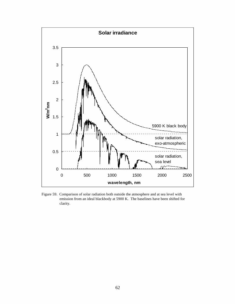
performing per its specifications. As a result, the sun was used as an alternate radiation source.
The sun is a nearly ideal blackbody source with a temperature of 5900 K (ASTM, 2003).
However, absorption by the atmosphere alters the spectral intensity received at ground level. A
comparison of solar irradiance with an ideal blackbody is shown in figure 59 (ASTM, 2003).
The chosen wavelengths were away from major water absorption lines to decrease the variability
in the calibration due to changes in atmospheric water vapor concentration.
3.7.5 Two-Color Imaging Pyrometer
The two-color imaging pyrometer employs two Vision Research Phantom 5.1 monochrome
cameras that image the explosive event along a single optical axis. A schematic of the two-color
imaging pyrometer is shown in figure 60. Focusing was accomplished using a single lens and
beam splitter assembly. The cameras were synched to a common time base by using one as the
“master,” which receives the trigger pulse and relays it to the second camera, the “slave.”
Cameras were fit with 10-nm narrow band-pass filters at 700 and 900 nm. The locations of the
filtered wavelengths relative to a blackbody at 2000 K are also shown in figure 60. System
resolution is dictated by the fixed effective focal length of the collection optics. Therefore, the
field of view (FOV) is adjusted by selecting the number of pixels in the image. The FOV must
be balanced with both the frame rate and exposure to ensure adequate signal-to-noise ratio. The
exposure time was the limiting factor in the camera setup due to the narrow band pass and
colinear optical-axis design. Cameras were set to 5000 frames/s and 196-μs exposure, with an
image size of 448 × 200 pixels. This rig was designed in-house.
62
Figure 59. Comparison of solar radiation both outside the atmosphere and at sea level with
emission from an ideal blackbody at 5900 K. The baselines have been shifted for
clarity.
Solar irradiance
0
0.5
1
1.5
2
2.5
3
3.5
0 500 1000 1500 2000 2500
wavelength, nm
W/m
2n
m
.
5900 K black body
solar radiation,
exo-atmospheric
solar radiation,
sea level
63
Figure 60. (Top) Schematic of the single-axis two-color imaging pyrometer showing the lens and
beam splitter arrangement. (Bottom) Band pass of each camera superimposed upon the
emission from a blackbody near 2000 K.
The experimental setup included a mechanism and procedure to precisely align the images from
both cameras. The procedure was repeated before each test to ensure that the passing blast wave
did not disturb the alignment. In addition, calibration images were saved to verify the alignment
offline. These images could be used to correct pixel registration but were deemed unnecessary.
Temperature calibration was achieved by recording images of a commercial blackbody source at
1255 K (Omega Engineering).
Video 1
Video
2
Filter 900nm
Filter 700 nmBeamsplitter
Lens Assembly
0
0.2
0.4
0.6
0.8
1
400 600 800 1000 1200
Wavelength (nm)
Black Body
700nm filter
900nm filter
64
3.7.6 Full-Color Imaging Pyrometer
The full-color imaging pyrometer, discussed in detail in section 2.3, uses the Bayer-type mask to
generate wavelength-specific emission data from a single camera (here, a Vision Research
Phantom 5.1 color camera) (Densmore et al., 2011). The advantage of this technique is that any
error associated with pixel registration between wavelength-specific images is virtually
eliminated. The disadvantage is that significant errors may be introduced if there is strong
discrete emission (e.g., for hydrocarbon/air flames, strong C2 or CH emission from nonsooting
flames). The Bayer-type mask generates subpixel output in red, green, and blue spectral regions
for each frame recorded by the camera. A MATLAB program generates the three separate pixel
arrays from each frame and ratios them pixel by pixel to create a 2-D temperature map from each
frame. A temperature movie is then created from the individual temperature maps.
In principle, any color camera with a digital readout may be used for temperature imaging,
provided something is known about any camera specific “on-chip” image processing. However,
each camera must go through a tedious calibration to map out the pixel response across the full
visible spectrum (Densmore et al., 2011). Camera calibration involves comparing subpixel
output with the output from a calibrated photomultiplier tube for narrow bandwidth radiation
over the full visible spectrum. Figure 61 shows a schematic of the Bayer-type mask in front of
the sensor element of a typical color camera and the resulting calibration graph for the camera
used in these measurements.
3.7.7 Wavelength-Resolved Emission Spectrograph
An often overlooked aspect of reacting systems pyrometry is the importance of discrete emission
(McNesby et al., 2004). As an example, figure 62 shows wavelength-resolved emission from
three types of ethylene/air diffusion flames (McNesby, 2005b). Most emission pyrometry
measurements assume a blackbody-like emitter with an emissivity that is invariant with
wavelength but less than unity; this is known as the graybody assumption (Planck, 1914).
However, as shown in figure 62, diffusion flames may show near-graybody behavior (the candle-
like flame) or a mixture of graybody and discrete emission (the coflow flame labeled “diffusion
flame”). They also may be nearly particulate free, in which case the emission is virtually all
from molecular and atomic emission (the opposed-flow diffusion flame labeled OPPDIF, which
shows little flame emission other than discrete C2 and CH band emission). Because this discrete
emission occurs in the visible (300–800 nm) and IR (1–30 μm) spectral regions, it presents the
greatest error source for the full-color imaging pyrometer. For this reason, a wavelength-
resolved emission spectrum is measured during every experiment using a fiber-coupled
spectrograph (Ocean Optics HR 4000, 1-nm resolution). The spectrograph collects and disperses
light for 50 ms following the received trigger. The reported spectrum will show any discrete
emission but does not tell when during the 50-ms collection window the emission occurred.
65
For results reported here, the graybody assumption was assumed to hold. As mentioned
previously, emissivity corrections for the most common particulate emitter (soot) have been
published in the open literature (Murphy and Shaddix, 2004). The explosive used here
(Composition C-4) is considered oxygen balanced, and the chemical makeup of the detonation
products is not known from experiment. Thus, wavelength-dependent emissivity corrections are
not employed here.
Figure 61. (Top) Schematic of the full-color imaging pyrometer showing the Bayer-type mask in front of the
sensor chip. (Bottom) Pixel calibration example from a Vision Research Phantom 5.1 camera.
66
Figure 62. (Top) Wavelength-resolved emission for three types of ethylene/air flames. (Bottom) Detail of emission from the OPPDIF flame showing emission bands due to CH and C2.
0
500
1000
1500
2000
2500
3000
3500
300 400 500 600 700
Wavelength (nm)
Em
issi
on
In
ten
sity
(a.
u.)
C2H4 candle
C2H4 diffusion flam e
OPPDIF C2H4-air
100
150
200
250
300
350
400
300 400 500 600 700
Wavelength (nanometers)
Em
issi
on
Inte
nsi
ty (
arb
.un
its)
C2 (Swan)
CH
67
3.7.8 Explosive Charges
Thirty-two spherical C-4 charges were exploded (twenty-nine 227-g charges and three 454-g
charges), and fireball temperature was measured using the multi-imaging rig. Five standoff
distances were used: three 12.7-cm charges, six 19.0-cm charges, six 31.8-cm charges, nine
44.4-cm charges (six 227-g charges and three 454-g charges), and eight 63.5-cm charges. Data
from three charges were incomplete due to either equipment malfunction or operator error. Only
three charges at a 12.7-cm standoff were measured, as other equipment (not reported here) was
damaged at this standoff distance. Based upon charge-to-charge variance within a test method,
we estimate temperature measurements reported here to have an uncertainty of between +/–100
K (integrating pyrometer, full-color pyrometer) to +/–200 K (two-color pyrometer).
3.7.9 Results: Three-Color Integrating Pyrometer
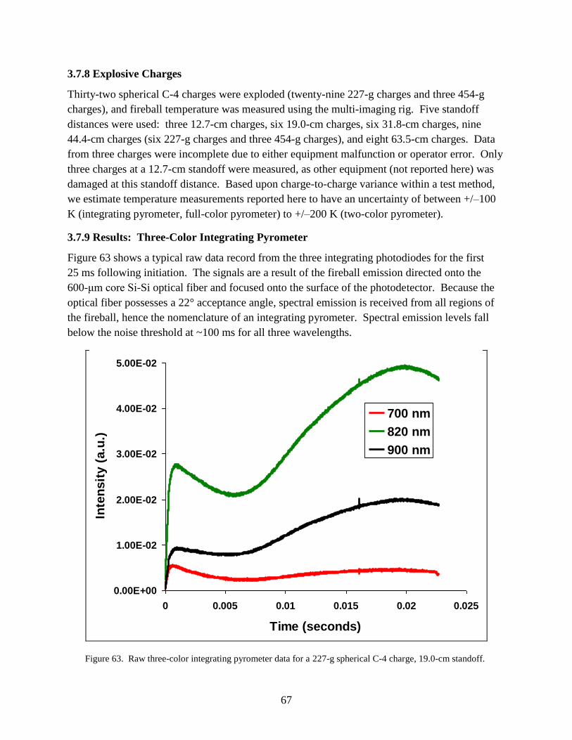
Figure 63 shows a typical raw data record from the three integrating photodiodes for the first
25 ms following initiation. The signals are a result of the fireball emission directed onto the
600-μm core Si-Si optical fiber and focused onto the surface of the photodetector. Because the
optical fiber possesses a 22° acceptance angle, spectral emission is received from all regions of
the fireball, hence the nomenclature of an integrating pyrometer. Spectral emission levels fall
below the noise threshold at ~100 ms for all three wavelengths.
Figure 63. Raw three-color integrating pyrometer data for a 227-g spherical C-4 charge, 19.0-cm standoff.
0.00E+00
1.00E-02
2.00E-02
3.00E-02
4.00E-02
5.00E-02
0 0.005 0.01 0.015 0.02 0.025
Time (seconds)
Inte
nsit
y (
a.u
.)
700 nm
820 nm
900 nm
68
Blackbody power output is governed by the Stefan-Boltzman law (equation 21) (Mehra and Rechenberg, 1982). Where W is the blackbody power output over all wavelengths, T is absolute temperature, A is the radiating surface area, and σ is the Stefan-Boltzmann constant. Because power output is proportional to the fourth power of temperature, the reported intensities will possess a larger contribution from hotter regions of the fireball. Therefore, the temperature calculated using the three-color pyrometer will be more indicative of a peak fireball temperature rather than an average fireball temperature.
4ATW . (21)
Three possible intensity ratios, and hence three possible temperature calculations, exist for the three-color integrating pyrometer: I700 nm/I820 nm – T12, I820 nm/I900 nm – T23, and I700 nm/I900 nm – T13. These three temperature calculations would be in reasonable agreement for a well-behaved experiment. In practice, however, T23 is generally in poorest agreement with the other calculated temperatures. This may be because the T23 temperature ratio possesses the smallest wavelength difference between factors in the calculation. Figure 64 shows the three calculated temperatures as a function of time for the raw data of figure 63. Additionally, the average calculated temperature profile is shown in figure 64. From here on, the remaining temperature data reported are the average calculated temperatures from the three intensity ratios.
Figure 64. (Left) Calculated three-color integrating pyrometer temperatures for a 227-g spherical C-4 charge at 19.0-cm standoff. (Right) Average temperature profile from the three calculated temperatures.
In what follows, standoff refers to the distance between the center of the unexploded charge to the table surface. As shown by figure 64, the highest temperature recorded occurs immediately after detonation. This is followed by an approximately exponential decay lasting 2 ms to a nearly constant temperature of 1/e times the initial temperature value. This constant temperature persists out to 100 ms, where the intensity signal eventually falls below the noise threshold. All charges detonated exhibited this same overall trend.
-200
1800
3800
5800
7800
9800
0 0.005 0.01 0.015 0.02
Time (seconds)
Te
mp
era
ture
(K
)
T12
T23
T13
0
2000
4000
6000
8000
0 0.005 0.01 0.015 0.02
Time (seconds)
Te
mp
era
ture
(K
)
-200
1800
3800
5800
7800
9800
0 0.005 0.01 0.015 0.02
Time (seconds)
Te
mp
era
ture
(K
)
T12
T23
T13
0
2000
4000
6000
8000
0 0.005 0.01 0.015 0.02
Time (seconds)
Te
mp
era
ture
(K
)
69
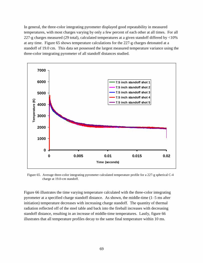
In general, the three-color integrating pyrometer displayed good repeatability in measured
temperatures, with most charges varying by only a few percent of each other at all times. For all
227-g charges measured (29 total), calculated temperatures at a given standoff differed by <10%
at any time. Figure 65 shows temperature calculations for the 227-g charges detonated at a
standoff of 19.0 cm. This data set possessed the largest measured temperature variance using the
three-color integrating pyrometer of all standoff distances studied.
Figure 65. Average three-color integrating pyrometer calculated temperature profile for a 227-g spherical C-4
charge at 19.0-cm standoff.
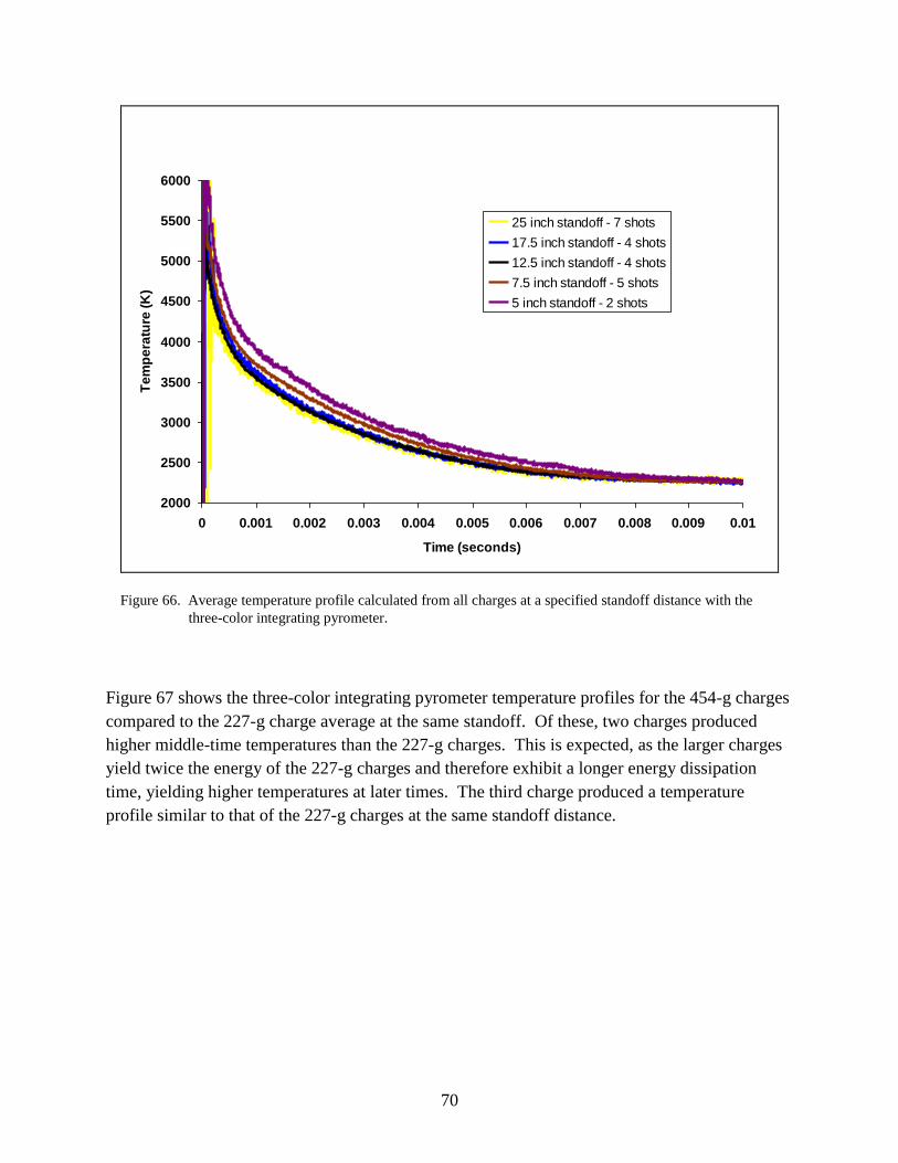
Figure 66 illustrates the time varying temperature calculated with the three-color integrating
pyrometer at a specified charge standoff distance. As shown, the middle-time (1–5 ms after
initiation) temperature decreases with increasing charge standoff. The quantity of thermal
radiation reflected off of the steel table and back into the fireball increases with decreasing
standoff distance, resulting in an increase of middle-time temperatures. Lastly, figure 66
illustrates that all temperature profiles decay to the same final temperature within 10 ms.
0
1000
2000
3000
4000
5000
6000
7000
0 0.005 0.01 0.015 0.02
Time (seconds)
Tem
pera
ture
(K
)
7.5 inch standoff shot 1
7.5 inch standoff shot 2
7.5 inch standoff shot 3
7.5 inch standoff shot 4
7.5 inch standoff shot 5
70
Figure 66. Average temperature profile calculated from all charges at a specified standoff distance with the
three-color integrating pyrometer.
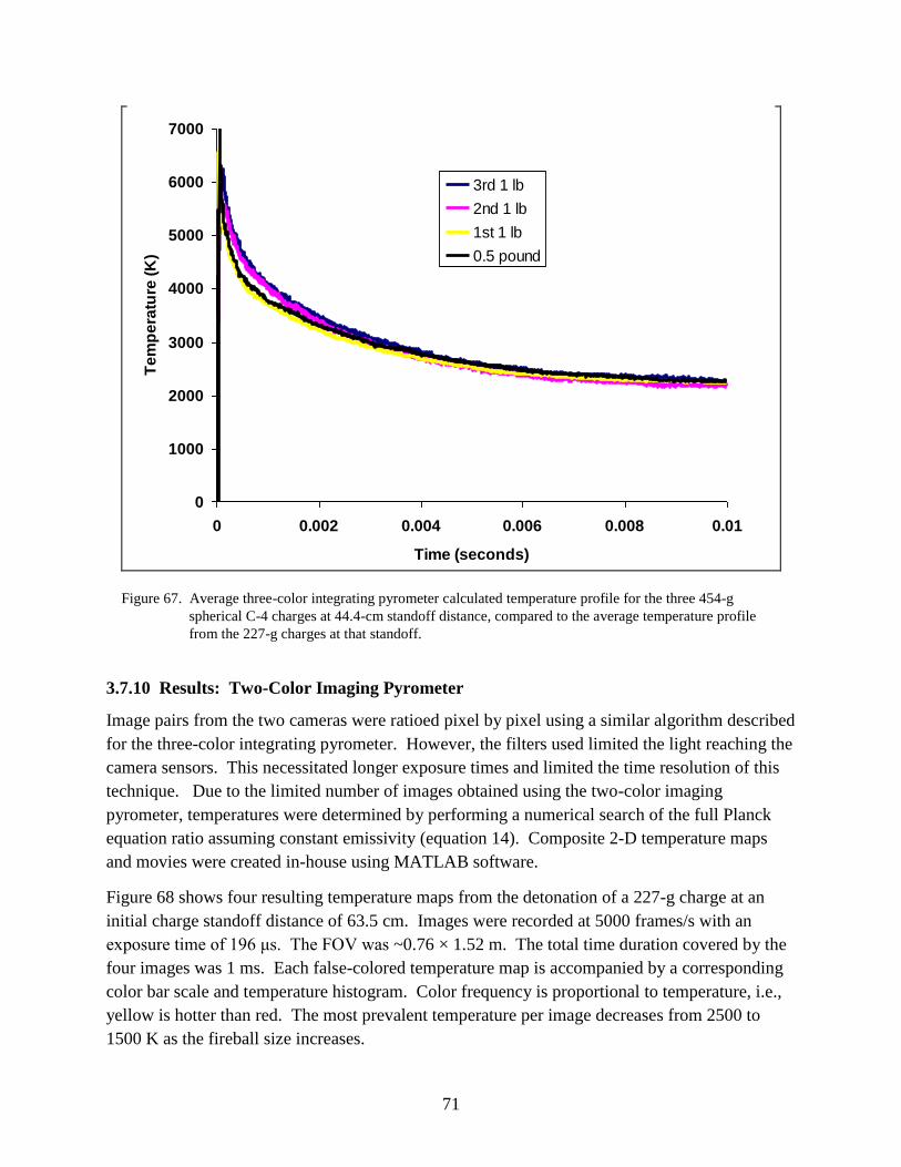
Figure 67 shows the three-color integrating pyrometer temperature profiles for the 454-g charges
compared to the 227-g charge average at the same standoff. Of these, two charges produced
higher middle-time temperatures than the 227-g charges. This is expected, as the larger charges
yield twice the energy of the 227-g charges and therefore exhibit a longer energy dissipation
time, yielding higher temperatures at later times. The third charge produced a temperature
profile similar to that of the 227-g charges at the same standoff distance.


![Nanoparticles For Soot Reduction [Div]](https://static.documents.pub/doc/80x56/61fbd2699871014c47523f3a/nanoparticles-for-soot-reduction-div.jpg)


