Experimental Protocol for Sedimentation Equilibrium Analytical Ultracentrifugation Andrea Balbo, Patrick Brown, and Peter Schuck Last updated in July 2007 This step-by-step protocol illustrates a sedimentation equilibrium (SE) study of a heterogeneous interaction between two proteins ‘A’ and ‘B’ forming a reversible complex. The goal of the experiment is the determination of the binding constant and the binding stoichiometry. It includes the determination of the molar mass of a non-interacting protein (or stable protein complex), and can be easily adapted to the study of protein self-association. Again, the details of the practical steps are given in conjunction with the workflow of the data analysis, which is closely tied to the experimental configuration. It will be assumed that a sedimentation velocity (SV) study of the same proteins and their mixture has taken place before, for example, using the SV protocol provided by us. It is essential that the reader be familiar with the document "general introduction to sedimentation equilibrium", which explains the conceptual and theoretical aspects, as well as the requirements with regard to sample preparation, purity, and amounts. The general introduction to sedimentation equilibrium also outlines the problem and strategies for the mathematical data analysis, which is a consideration indispensable for the successful experimental setup. Modern analysis techniques gain substantially in information and precision from fitting several experimental data sets globally. Since this introduces an increasing number of fitting parameters, it is imperative to take advantage of available constraints, such as mass conservation and relationships between the loading concentrations from different sample solutions, which can be generated by appropriate experimental designs. This is described in detail in Vistica et al . The protocols have been written here in an effort to make the experiment most informative. By following the protocol, one is able to generate several parameter constraints making the analysis most manageable. Much care and foresight should go into the planning, preparation, and data acquisition stages, to minimize errors and noise. Also, in the design and execution of the experiment it is important to already anticipate the later data analysis stage, in order to obtain reliable, high quality data with sufficient information to determine the thermodynamic parameters precisely. Other resources that can be found here are a flow - chart for AUC experiments , as well as tables containing a grid for buffer selection with different optical systems , configurations for SE and SV experiments with different optical systems , as well as AUC strategies commonly employed for selected typical problems . Hands-on training in the techniques described here can be obtained from the Workshop on Hydrodynamic and Thermodynamic Analysis of Macromolecules with SEDFIT and SEDPHAT at the National Institutes of Health, which takes place twice a year in Bethesda, Maryland. Page 1 of 21 SEProtocols 8/31/2009 file://D:\workshops\Uppsala\CD\Experimental\seprotocols.htm
Transcript
Experimental Protocol for Sedimentation Equilibrium AnalyticalUltracentrifugation
Andrea Balbo, Patrick Brown, and Peter Schuck
Last updated in July 2007
This step-by-step protocol illustrates a sedimentation equilibrium (SE) study of a heterogeneous interaction between two proteins ‘A’ and ‘B’ forming a reversible complex. The goal of the experiment is the determination of the binding constant and the binding stoichiometry. It includes the determinationof the molar mass of a non-interacting protein (or stable protein complex), and can be easily adapted to the study of protein self-association. Again, the details of the practical steps are given in conjunctionwith the workflow of the data analysis, which is closely tied to the experimental configuration. It willbe assumed that a sedimentation velocity (SV) study of the same proteins and their mixture has takenplace before, for example, using the SV protocol provided by us.
It is essential that the reader be familiar with the document "general introduction to sedimentation equilibrium", which explains the conceptual and theoretical aspects, as well as the requirements with regard to sample preparation, purity, and amounts. The general introduction to sedimentation equilibrium also outlines the problem and strategies for the mathematical data analysis, which is a consideration indispensable for the successful experimental setup. Modern analysis techniques gainsubstantially in information and precision from fitting several experimental data sets globally. Since thisintroduces an increasing number of fitting parameters, it is imperative to take advantage of availableconstraints, such as mass conservation and relationships between the loading concentrations fromdifferent sample solutions, which can be generated by appropriate experimental designs. This isdescribed in detail in Vistica et al.
The protocols have been written here in an effort to make the experiment most informative. Byfollowing the protocol, one is able to generate several parameter constraints making the analysis mostmanageable. Much care and foresight should go into the planning, preparation, and data acquisitionstages, to minimize errors and noise. Also, in the design and execution of the experiment it is importantto already anticipate the later data analysis stage, in order to obtain reliable, high quality data withsufficient information to determine the thermodynamic parameters precisely. Other resources that can befound here are a flow-chart for AUC experiments, as well as tables containing a grid for buffer selection with different optical systems, configurations for SE and SV experiments with different optical systems, as well as AUC strategies commonly employed for selected typical problems.
Hands-on training in the techniques described here can be obtained from the Workshop onHydrodynamic and Thermodynamic Analysis of Macromolecules with SEDFIT and SEDPHAT at theNational Institutes of Health, which takes place twice a year in Bethesda, Maryland.
0. Instrumentation needed * Analytical Ultracentrifuge (Beckman Coulter) equipped with absorption optical scanner (ABS) and
optionally Rayleigh laser interferometer (IF) imaging system * Spectrophotometer (preferably dual-beam, any supplier) may be required for the determination of the
protein concentration via UV absorbance * Densitometer (Anton Paar) may be required for measuring the solvent density if non-tabulated buffer
components are used (tabulated values are available for most common buffers and salts)
* Computer (PC) equipped with software to perform the data analysis (this should not be a PC simultaneously running the ultracentrifugal data acquisition to avoid interference):
(1) SEDFIT and SEDPHAT for transforming and analyzing the sedimentation equilibrium data;
(2) SEDNTERP for calculating the protein partial-specific volumes and extinction properties, as well as buffer density;
(3) general purpose software to store screenshots for documentation (MS Word, powerpoint or equivalent)
(4) internet connection to consult the SEDPHAT getting started tutorials, the step-by-step tutorials for sedimentation equilibrium analysis, the command reference manual, and the SEDFIT/SEDPHAT search bar. For an introductory overview, point your web-browser to http://www.analyticalultracentrifugation.com/sedphat/sedimentation_equilibrium_for_interacting_sy
I. Planning the Experiment 1. Collect all prior knowledge. Although not all of this information is essential, and some may not bepossible or fascile to obtain, it can often be helpful during and after an analysis. It helps to have thisinformation in the planning stages for determining rotor speeds, time to equilibrium, etc.; also during theanalysis stage as far as inputting starting guesses for the fitted parameters, and after an analysis todetermine if fitted parameters make sense.
a. Obtain the amino acid sequence(s) of the analytes. (Essential)
The molar mass as well as the extinction coefficient at 280 nm (and 250 nm) and the valuescan usually be calculated from a known amino acid sequence (via SEDNTERP). For proteinsthat are known not to self-associate, the buoyant molar mass (essentially the ) values of the individual proteins will be measured in this protocol, but it is useful to compare this value withthe theoretical sequence value. Also, inquire about whether any free cysteines are known to bepresent as these can lead to irreversible crosslinking.
b. Obtain mass spectrum. (Optional, but sometimes essential)
Ensure agreement between mass calculated from composition with that obtained by massspectrometry. Some possible explanations for disagreement include: proteolytic cleavage, post-translational modification, irreversible aggregation, etc. For glycoproteins, the determination ofthe carbohydrate mass fraction by mass spectrometry is desirable, in order to calculate a goodestimate of the partial-specific volume of the glycoprotein.
c. Observe size-exclusion chromatogram. (Highly desirable)
Knowing where a protein of specific molecular weight elutes can give insight into theasymmetry of the protein (not important in SE but is in SV) as well as the possible heterogeneityof the collected fractions. Even more importantly, size-exclusion chromatography should be thelast purification step, if at all possible (see below).
d. Observe a PAGE gel image. (Essential)
Native gels and denaturing gels under reducing/non-reducing conditions can be useful inestimating protein mass, and in observing the presence of higher-order complexes and/or crosslinked aggregates.
e. Understand the composition of the buffer. (Essential)
Useful information may be how the buffer was obtained, whether it is filtered dialysate or flow-through of the SEC column. Are there any additives that can be observed with the opticaldetection system which will contribute to the shape of the gradient or that will affect the mannerin which the protein sediments and diffuses. Measure or calculate buffer density and viscosityfor the temperature at which the SE experiment will be performed. See below section I.3.
f. Other information: (Optional)
Knowledge of the stability of the protein is important for designing the experiment. If theprotein is prone to degradation or aggregation at room temperature it may be more desirable toacquire data at lower temperatures or for shorter time periods (using shorter solution columns orat fewer rotor speeds). Additionally, this information may be useful in the analysis stagewherein inclusion of proteolytic fractions or discrete aggregates can be incorporated into themodel.
It can be useful to consider results from other biophysical experiments that have been performedon the system of interest (or similar systems) as a guide to reasonable estimates of affinity orstoichiometry in the planning and/or analysis stages.
It may be helpful from a troubleshooting perspective to understand the expression system, andsteps taken in the purification process.
2. Conduct a SV experiment in order to assess the purity of the sample and to gain some qualitative assessment of the concentration dependence of the association state. Generally, purity of better than95% is required for SE. Small molar mass impurities (e.g. with masses in the range of a few percent ofthe proteins of interest), which frequently go undetected by SDS-PAGE, will complicate the analysis and should be removed, if possible. Irreversible small oligomeric aggregates will generally also limitthe precision of the binding parameters to be measured. Therefore, size-exclusion chromatography is highly recommended as the last preparative step. Contamination with very large aggregates, distinctly
larger than the molar mass of the complex, can usually be tolerated. The SV run should be conducted ata wide range of sample concentrations, such that it will provide insight into the oligomeric state of eachprotein in solution and the detection of reversible self-association of the two components. It will also permit crude estimation of the binding constant (KD* – e.g., an empirical estimate of the concentration at which the AB complex is half-saturated). This will greatly help in planning the sample concentrationsand the rotor speeds for the SE experiment.
3. Consider the buffer composition. Phosphate buffers are transparent in the far UV and are suitablefor both ABS and IF detection. For example, PBS (phosphate buffered saline) will work well. Whenusing other buffers, see Table 1 and Table 2. If the buffer conditions and the protein extinction do notgovern the choice of the detection system, use the IF system. Make sure you know all the components of the buffer solution being used. Then, measure the density and viscosity of the buffer, at the actualAUC run temperatures, with the densitometer and viscosimeter, respectively, or calculate them withSEDNTERP. (The viscosity is strictly required only for SV experiments, but can be useful when usingadditives, such as glycerol or sucrose, in SE that can increase the time required to attain equilibrium.) As a preliminary step, it might be necessary to establish sedimentation/optical properties of the bufferbefore analyzing the actual proteins, if, for example, detergents or other sedimenting buffer componentsare present at concentrations leading either to signal gradients or density gradients. Buffer conditionsare slightly less restrictive for SE with regard to components that can create density gradients at thehigher rotor speeds of SV: For example, a small percentage of glycerol can be tolerable in SE using theABS optics, provided the potential effect on from preferential protein hydration and the extendedequilibration time is taken into account. As in the SV experiments (Step I.2.), a chemically identical reference buffer is required when using IF optics. Measure the buffer density or use SEDNTERP tocalculate the appropriate value.
4. Choose the rotor and centerpieces. The 8-hole rotor and double sector centerpieces are therecommended option.
The double sector centerpieces allow for longer solution columns than the 6-channel centerpieces. While requiring longer time to reach equilibrium, longer solutions columns provide for increasedcurvature and more data points in the gradient which leads to better precision in the analysis. When 6-channel centerpieces cannot be avoided due to the large number of samples that need to be run, fill themwith the maximum volume (130 – 140 microliters).
The 8-hole rotor allows for at least twice as many samples to be analyzed in one experiment than by using the 4-hole rotor. If using an 8-hole rotor, reserve one cell for each of the individual proteins to runas a control, and use the 5 (or 6) remaining cells for mixtures. With a 4-hole rotor, consider using three 6-channel centerpieces to increase the number of samples. If these options are not available and theindividual components have to be studied in a separate run, note that small differences in the purity orpresence of irreversible aggregates from different preparations or from different time-points can be confused with and correlate with the detection of putative heterogeneous complexes. In practice, thiscan be a problem, particularly for weak interactions.
5. Select approximate sample concentrations to span a range that will generate different relativepopulations of free and complex species: For hetero-associations with unknown stoichiometry, it can be advantageous to choose a constant concentration of ‘A’ 2fold to 5fold greater than the estimated KD*, and to titrate constant ‘A’ in different samples with variable amounts of ‘B’ to generate a range of molar ratios comprising the suspected possible stoichiometries. (The constancy of loaded amounts of ‘A’ can later serve as a powerful constraint on the data analysis.) This may be combined with a second set of A
and B at the same molar ratios used initially, but at a concentration of ‘A’ several-fold below KD*. In contrast, if the stoichiometry is known, it can be advantageous to make a stock mixture at aconcentration of > 10fold KD* with a molar ratio equal to the complex stoichiometry, and to generate the different samples by serial dilution to span a large range of concentrations. (Here, the constancy ofthe molar ratio generates a useful constraint for the data analysis.) If the available maximal sampleconcentrations are too low (e.g. only one tenth of KD*) adjust the following protocol by using a longer solution column, tolerating the longer equilibration time but taking advantage of the concentrating effectof the centrifugal field. The dynamic range of the optical system (see Table 1) must be considered forselecting sample concentrations.
6. Choose the optical detection and double-check the sample concentrations with regard to optical detectability. The key for selecting the optical system is to generate SE profiles in such a way that the contributions from free species, which attain relatively shallower exponential distributions, and complexspecies, which generate relatively steeper exponentials, can all be detected and distinguished (see theintroduction to SE): Proteins vary greatly in the number of tyrosine and tryptophan residues, andtherefore in their extinction spectrum in the far UV. Because the ABS system can take advantage of thisdifference to help distinguish between the components ‘A’ and ‘B’, ABS with multi-wavelength analysis is usually preferred. Obviously, this technique will be more powerful for protein/nucleic acidinteractions, or if one of the interacting components has an intrinsic chromophore in the near UV or VISor if an extrinsic label can be attached. Attaching an extrinsic label is frequently very useful if the molarmasses of ‘A’ and ‘B’ differ by less than 20% or more than 80%. However, in many cases this may not be necessary when SE data are obtained at multiple rotor speeds in conjunction with mass conservationanalysis (a technique described in the following).
For the choice of the protein concentrations for ABS detection, if consistent with the order of magnitudeof KD*, and the considerations described in Step I.5., maximize the dynamic range of the ABS system at the wavelengths of 230 nm, 250 nm, and 280 nm: This can be achieved in samples with totalabsorbances of 0.1 OD230, 0.2 OD280, 0.5 OD280, and 0.5 OD250. Note that the centrifugal field will create a gradient locally decreasing or increasing the concentrations several-fold. Higher concentrations can be used, for example, with very high KD*, but this may require the use of the IF optics to not beconstrained with the limited linearity of the ABS optics. For the two individual protein samplesincluded as controls in the same run, choose a concentration of 0.5 OD280. This will permit the determination of their extinction coefficients at 230 and 250 nm.
The use of the ABS system may be prohibited by the solvent conditions, or it may not provide asufficient dynamic range of protein concentrations for the detection of weak interactions. Also, one orboth of the proteins under study may not have a sufficiently high extinction coefficient to generatesignals > 0.05 OD at any or all of the absorbance wavelengths permitted by the buffer system. In thiscase, the IF system can be used, with the considerations for sample concentrations as outlined above(Step I.5.).
Maximum information can be gained if the IF system is used in conjunction with the ABS system,which improves the distinction between the two proteins in a multi-signal analysis. Note that the use of the IF system for SE will require the mechanical stabilization of the cell assembly (Step II.2a.). In the combination of IF with ABS data, in particular if the solution volumes and rotor speeds are used assuggested in this protocol, the radial-dependent baseline can be computationally determined and waterblanks are not essential.
7. The choice of the sample volume and rotor temperature is dictated mainly by the protein size and stability. Except when studying interacting systems with very slow chemical rates (frequentlyencountered with very high affinity systems), the sedimentation time is governed by the diffusion of theproteins throughout the solution column. As a standard choice, use 170 microliter samples and expectequilibration at the first speed within 48 hours (usually less time is required at the following,sequentially higher rotor speeds). True attainment of sedimentation equilibrium must be checkedexperimentally (see below). To avoid longer equilibration times required for larger protein complexes >200 kDa, usually the sample volume is decreased to 140 – 150 microliters. For samples that do not possess sufficient stability for attaining equilibrium at three rotor speeds, 100 – 120 microliter samples can be used. (Alternatively, shorter column techniques are available, but they only provide informationon the approximate average molecular weight as a function of loading concentration, which does notprovide as much detail as the long-column technique and requires a different analytical strategy thandescribed in this protocol [see, e.g., molecular weight isotherm analysis in SEDPHAT].) On the otherhand, when studying small proteins (e.g., < 5 kDa) or peptides, larger solution columns of up to 400microliter may be advantageous to generate equilibrium gradients with sufficient curvature at theaccessible rotor speeds. In this case, the higher diffusion coefficient of smaller species leads to an onlymoderate increase in equilibration time.
To shorten the time to attain equilibrium, an initial overspeeding period for a few hours at three-fold the first equilibrium rotor speed can be used, but the concentration profiles should be monitored so as not toexceed a value two or three times the loading concentration at the bottom of the cell (this is described inStep III.3. below).
Usually, the rotor temperature is an important factor for the stability, and unless thermodynamicconsiderations prescribe the use of a particular temperature (the binding constant is temperaturedependent following RT ln(KA) = ΔG = ΔH – TΔS), low temperatures such as 4 – 8 °C are recommended.
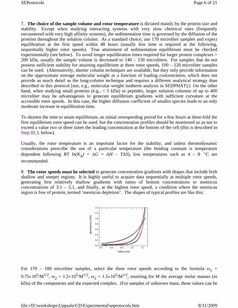
8. The rotor speeds must be selected to generate concentration gradients with shapes that include both shallow and steeper regions. It is highly useful to acquire data sequentially at multiple rotor speeds,generating first relatively shallow gradients with ratios of bottom concentrations to meniscusconcentrations of 3:1 – 5:1, and finally, at the highest rotor speed, a condition where the meniscus region is free of protein, termed ‘meniscus depletion’. The shapes of typical profiles are like this:
For 170 – 180 microliter samples, select the three rotor speeds according to the formula ω1 =
0.75×10⁵/M1/2, ω2 = 1.2×10⁵/M1/2, ω3 = 1.5×10⁵/M1/2, inserting for M the average molar masses (in kDa) of the components and the expected complex. (For samples of unknown mass, these values can be
estimated from the previous SV experiment, or from the initial slopes in an Archibald analysis of theearly experimental SE data close to the meniscus and bottom (see Schuck & Millar 1998), available in SEDFIT.) For different sample volumes, measure the new column height l from initial scans and use the
formula to correct the value from those given above. A slightly higher valuefor the highest rotor speed generating steeper gradients can be applied when using the IF optics.
9. If unsure about column lengths and rotor speeds, simulate SE data. To assist in selecting the appropriate configuration for the experiment, you can use the ‘Generate’ function of SEDFIT to assess the shape of the predicted SE profiles by simulating the approach to equilibrium at a given rotor speed. If this is based on realistic molar mass values and sedimentation coefficients of the free and complexspecies (for example, assuming equal concentrations of each), this will also indicate the expectedminimal time to attain equilibrium.
A more advanced simulation with SEDPHAT is also possible, in which realistic levels of noise areadded to theoretical equilibrium profiles calculated on the basis of hypothetical values for the bindingconstants. Re-analysis of this theoretical data set can be used to judge if the SE run will provide enoughinformation to determine the correct binding constants with acceptable error estimates. The latterrequires slightly more familiarity with the software than introduced in the present protocol, and thereader is referred to the extensive SEDPHAT help section athttp://www.analyticalultracentrifugation.com/sedphat/sedphathelp.htm. In brief: (1) Use SEDFIT to generate a template data set for a non-interacting systems using the same rotor speeds and column lengths as those to be tested, with a dummy single sedimenting species model; (2) Make the xp-files and load the data in SEDPHAT as if doing an analysis of an interacting system; (3) choose the appropriatemodel and enter hypothetical concentrations and binding constants; (4) switch off any baselineparameters in the xp-files; (5) execute a RUN command; (6) Use the function "Save Fit Data" to savethe theoretical curves. Finally, a similar procedure in SEDPHAT can be used to examine the kinetics ofthe approach to equilibrium for an interacting system with given kinetic rate constants of theinteraction. This proceeds similarly as the SE simulation, but using a sedimentation velocity templatefor the approach to equilibrium.
II. Preparing the Analytical Ultracentrifuge and the Cell Assembly 1. Assemble the cell components according to manufacturer’s instructions. For the IF optics, sapphire windows are required, for the ABS system, use quartz windows. When assembling the components,determine if the window gaskets obscure the corners at the bottom of the sample and reference sectors. Frequently, some trimming with scissors is required to eliminate any shadow in the light path from thegaskets. This is very important in SE, because otherwise the region of the steepest gradients with thehighest information content in SE cannot be observed. Select double-sector charcoal filled Epon centerpieces. (There are several alternatives: six-channel centerpieces permit more samples to be studied, but only at lower sample volume; for the IF optics, centerpieces with dual filling holes areavailable, or six-channel external loading centerpieces, which make thorough rinsing of the cellassembly easier after the ‘aging’ process (see next step)).
2a. For the IF optical detection only, mechanical stabilization of the cell assembly is required. Due to the exquisite sensitivity of the IF system to optical pathlength differences on the nanometer scale,rotor-speed and time-dependent signal offsets result from small deformation induced by the gravitationalstresses. If these offsets are not removed or are unaccounted for in the analysis it may lead to erroneous
This can be prevented by the following pre-conditioning procedure: a) Assemble the cells and torque to 120 – 140 inch×lb. Fill the cells with 200 microliters of water (the volume must be greater than the sample volume for the following SE experiment) and seal them. b) Insert the assemblies into the rotor, carefully align them, and centrifuge for 1 hour at 50,000 rpm. c) Stop the run and take the cell assemblies out of the rotor. d) Re-torque the cells, and observe if the screw rings have slightly loosenedas a result of the centrifugation. e) Repeat steps b, c and d until no movement of the screw ring is required to reach the proper torque. f) Insert the cell assemblies in the rotor, insert the rotor in the centrifuge chamber, and install the optical arm. g) Accelerate the rotor to 50,000 rpm and configure theIF optical system. h) Set up ten alternating rounds of 2 hours centrifugation at 50,000 rpm and 1 hourcentrifugation at 3,000 rpm. During each 50,000 rpm run, take a series of 10 IF scans in 5 minuteintervals. This step can be conveniently set up as an ‘equilibrium method’ in the AUC operating software to run overnight. i) Establish that the scans in successive series show no change in RMS error,indicating that no further mechanical change in the cell assembly occurs. The newest version ofSEDFIT allows users to determine whether successive scans overlay. This can be done by loading allthe IF scans and selecting “Sort EQ data” in the Loading Options menu. Answer “no” to the next two windows (‘subtract blank scan?’ and ‘make xp files?’) and a plot of appears with Y= rms error and X=time. This completes the mechanical stabilization or ‘aging’ of the cells.
If the cells are to be stored before use, leave them filled with water. Important: do not disassemble thecells before their use. Only immediately before use, the remaining water can be aspirated by suctionapplied to small diameter tubing, and then filling the sample and reference solutions, as described in thefollowing step.
2b. Acquire speed-dependent water blank scans for each cell. For the IF system only: Take ‘aged’cells (still loaded with 200 μl water per sector), insert the rotor and mount the optical arm, andcentrifuge at the first rotor speed selected for the SE experiment. Adjust the parameters for the IF opticsin the ‘Laser setup’ for each cell (for criteria see Step III.8. of the SV protocol). After 1 hour of centrifugation, take a set of 10 IF scans (in the velocity mode with time interval 10 sec). Repeat at allother rotor speeds selected for the SE experiment. These scans will serve as ‘water blanks’.
Important: The settings of the IF optics, the particular rotor used, and the timing of the laser mustremain unchanged for the remainder of the SE experiment for the water blanks to be valid. In order toreproduce these settings, make a note of each of the laser setup parameters for each cell. (This condition is certainly a weak point of using experimental water blanks, since removal and re-insertion of the cells into the rotor and the laser attachment into the rotor chamber may cause slight shifts. However, in particular when these steps are performed by thesame operator, the reproducibility is usually sufficient.)
Stop the run, carefully remove the water from the cell assemblies through the filling holes, withoutcausing any mechanical change in the assembly. For example, use suction applied through a small tubeconnected to a vacuum flask. Rinse both sectors of the cell with reference buffer and remove thebuffer. This will prevent small changes in the buffer composition from residual water when filling thecell assembly. Then load with sample and reference buffer solutions.
This step II.2b is not essential in experiments with a sufficient range of rotor speeds and column length(the default recommendations) to permit computational determination of the radial-dependent baseline, in particular when IF and ABS detection are combined. However, the experimental determination canbe both a safe-guard against unexpected profiles that do not meet the computational requirements, and atest for consistency of the data analysis.
III. Sample Preparation and Starting the Run 1. Mix the samples in Eppendorf tubes. Fill the cell assemblies with the sample at the volumesplanned in Steps I.5., I.6., and I.7. For the ABS system, fill the reference buffer to a volume 10 microliters larger than that in the sample sector. When using the IF system or a combination of ABSand IF, precisely match the reference buffer in volume (and chemical composition) to the sample. Sealthe cell assemblies as described in Step III.3 of the SV protocol.
2. Insert the cell assemblies into the rotor, weigh and install the counterbalance, and align the cells atthe scribe marks. Insert the rotor into the rotor chamber and mount the optical arm. (NOTE: whenacquiring absorbance data below 400 nm, the high-pass filter lever should be parallel with monochromator housing.) Evacuate the chamber, and set the desired temperature on the centrifugepanel.
Determine whether or not the optical system is reliably radially calibrated. If not, select a rotor speed of4,000 rpm, and perform the radial calibration of the required optical system. (Note that this can be donewith the sample in place for a SE experiment, in contrast to the SV experiment.) A new radialcalibration should be necessary only after the optical system has been changed or serviced, and withunchanged optical setup, the calibration should be valid for different rotors.
When the vacuum permits, accelerate the rotor to the first (lowest) rotor speed selected in Step I.8. Note that the equilibrium experiment does not require the temperature equilibration period that is essential forSV.
3. In exceptional cases when studying proteins of limited stability, an initial overspeeding periodmay be required to shorten the experimental time. For overspeeding, increase the rotor speed to threefold the first selected equilibrium speed, and set up a sequence of scans (e.g., absorbance at 280nm) as a velocity method to monitor the concentration gradients. After a few hours, when theabsorbance signal near the cell bottom has approximately doubled, stop the scanning and drop the rotorspeed to the first equilibrium speed. (Any sedimentation creating excess concentration at the bottom ofthe solution column will significantly prolong the experimental time and may lead to irreversible orslowly reversible aggregate formation.)
4. Prepare the scan settings file on the AUC control computer. Specify the rotor type, set the centrifugation time to ‘hold’ mode, and set the run temperature. Set the parameters of each cell to theabsorbance (and/or interference, respectively) equilibrium mode. Set the radius interval for scanningfrom 6.6 to 7.25 cm (for 180 microliter columns), and the wavelength to 280 nm.
5. In the ‘Options’ settings, select ‘Acquire intensity data instead of OD data’. This will separately store the radial-dependent light transmission through the reference and the sample sector, respectively,and provide a rational criterion for the appropriate data analysis range. The intensity scans (which willbe saved in ‘*.ri*’ files) can be transformed to absorbance scans easily at any later time with SEDFIT without loss of information. In the same menu, set the number of overlays to 3.
6. For each cell, specify the scan ‘Details’: Enter as additional wavelengths 250 nm and 230 nm. Setthe radial step size to 0.001 cm and request 20 replicates in the stepping mode. Specify if using the 2(default), 6, or 8 channel centerpieces. Specify a new directory name for data storage. When using theIF system, set the inside and outside radius to encompass the complete solution column. Do not change
the laser settings after water blanks have been acquired. Verify the ‘Laser Setup’ parameters are as noted in Step II.2b. Only if no water blanks were taken (for computational determination of the radial-dependent baseline), set up the laser timing and imaging parameters in the ‘Laser Setup’ (for criteria see III.8. of the SV protocol) and make a note of the settings for each cell.
7. Save the scan settings file and start a single scan to verify the quality of scans. When the ABS data acquisition is in intensity acquisition mode, as recommended above, two profiles will be shown foreach cell: the radial-dependent reference transmission and the sample transmission. Both meniscishould be visible; they can be identified as a local dip in the transmitted light. The scans should extendfrom the air-to-air region in front of the meniscus to the shadow region at the end of the solutioncolumn. The radial position r* near the bottom of the cell where the reference intensity starts to decline (from the shadow of components of the cell assembly) will mark the maximum radius that can bepotentially considered for analysis. Write down this value for later use. The transmitted intensitythrough the sample, at least for one of the selected wavelengths, should be between 10% and 90% of thereference intensities. With time, the intensity transmitted through the sample close to the meniscus willincrease, approaching that of the reference, and will strongly decrease or disappear close to the bottom,indicating the accumulation of the protein.
8. Set up and run a ‘Method’ for scanning. Described in the following are two alternative routines forsetting up a method scan. The first routine involves manually stepping the instrument to the nexthighest speed once data for all cells in sedimentation equilibrium has been collected. The secondroutine allows for a scheduled automatic increase in rotor speed.
8a. Routine 1: In the ‘Methods’ menu for SE, start with the lowest rotor speed and set up a sequenceof scans in six hour intervals for several days (‘delay condition’ is 6:00, ‘number of scans’setting is 1, and enter the desired run temperature). Start a ‘Method’ scan. Allow scanning to continue at this first speed until the material in the cells reach sedimentation equilibrium.
To check for this condition in real-time, all scans collected by the absorbance optics or all scanscollected by the interference optics (but not both types) can be loaded into SEDFIT. Under the“Options/ Loading Options” drop-down menu select “Test Approach to Equilibrium”, answer the resulting dialog boxes that appear accordingly (see SEDFIT help website). A plot will begenerated which shows the root-mean-squared difference between each scan acquired for eachcell and wavelength compared to the latest respective scan that was acquired. This plot will beautomatically updated once new scans become available. The experiment should be consideredto be at equilibrium once the rms difference asymptotically approaches a constant value. Further, this value should be at or below the level of noise in data acquisition (< 0.01).
A rigorous criterion can be formulated with the F-statistics, requiring that the rmsd difference between successivescans to be statistically indistinguishable. However, the visual inspection of the entire time-course of the approachto equilibrium, which should be a smooth asymptotic approach, is equally important. For an example, seehttp://www.analyticalultracentrifugation.com/eqtest.htm.
A frequent beginners mistake is to use too short time intervals for checking equilibrium (e.g., 3 hour intervals forlong solution columns leaves too little time for sedimentation to proceed), and only to consider the differencebetween two successive scans. This can easily mislead to belief sedimentation equilibrium has been reached, when,in fact, it may still be significantly different from the true final distribution. It is important to note thatconcentration gradients that are still significantly away from equilibrium may already look quite exponential, andthe deviation may not be caught in the data analysis and result in false parameter values. Therefore, getting a goodfit in the data analysis cannot be taken as a confirmation of being sufficiently close to sedimentation equilibrium.
If the rms difference does not appear to have leveled off at a constant value, sedimentation
equilibrium is not yet attained and centrifugation at the current rotor speed must be continued. Note that in this assessment the radial range considered for comparison will play a role, andshould exclude the regions of optical artifacts and non-linear instrument response.
If equilibrium is not attained after what should have safely been sufficient time (e.g., two or three times the normaltime required), consider whether proteolytic degradation or aggregation may take place, which will continuouslychange the distribution of soluble material. In this case, one may have no choice but to work with imperfectlyattained equilibrium, accept the data and to proceed with the experiment, hoping that the sample degradationproceeds at a timescale much slower than sedimentation and diffusion of the sample, such that the loss of materialis ‘adiabatically proceeding through mechanical sedimentation equilibria’ (– a case with the only disadvantage of not being able to use mass conservation constraints in the analysis). To confirm the presence of proteindegradation, see Step III.10. Finally, it is advisable in this case to perform the interaction study by sedimentationvelocity, which takes place on a much shorter time-scale and offers more tools to address the problem of slowprotein degradation.
If equilibrium has been reached, stop the scanning and in the ‘Methods’ box, replace all previous rotor speeds, with the next higher speed. When using the IF optics, verify that the laser settingsremain unchanged. Start a new set of scans and verify that this will accelerate the rotor. Repeatthis step for remaining rotor speeds.
8b. Routine 2: As an alternative to 8a: For proteins that are known to be sufficiently stable, and inthe absence of factors that could significantly extend the centrifugation time (e.g., high viscositybuffer, very large protein complexes > 200 kDa, very elongated protein shape leading to anunusually small diffusion coefficient, or working with diluted stock mixtures of reactants thatexhibit very low chemical off-rate constants), the ‘Methods’ for the SE can be configured in one step to go through a sequence of rotor speeds. For 170 microliter columns, start with the lowestrotor speed and request 8 scans in 6-hour intervals. Continue with the next higher rotor speeds,for each requesting 6 – 8 scans in 6-hour intervals. (Frequently the equilibrium at the second andthird rotor speed is attained faster than the first.) At the end of the highest rotor speed, append aline with the delay condition ‘hold’. Start the ‘methods scan’. This will automatically collectthe necessary set of scans and switch the rotor speeds during the next several days.
Attainment of equilibrium can be observed during the run with SEDFIT as described above,and/or verified after the run is finished (or better while the highest rotor speed is still on hold). The obvious disadvantage of this routine is that it does not offer the possibility of extending thesedimentation time retroactively, except for the highest rotor speed. However, if, during the run,it is found that equilibrium is not going to be properly attained (for example, if from the time-course of rmsd difference to the last scan it can be discerned that not sufficient time is availablefor the asymptotic approach, or the rmsd differences are still too high), this scan ‘Method’should be stopped, and restarted with a modified protocol that allows for sufficient scans. (Inthis case, account for the fact that a number of scans have already been taken.)
9. Stop the run, once equilibrium profiles at all rotor speeds have been acquired.
10. Check the stability of the protein. It is generally advisable to recover the sample for analysis by SDS-PAGE or mass spectrometry. This can show if proteolytic degradation has occurred. Alternatively, the solution can be re-suspended by carefully shaking the cell, and a short-column SV experiment can be conducted with the c(s) analysis indicating the solution state of the protein mixtures. (The latter is not done routinely).
At this point, if further study of the sample by dynamic light scattering is desired, the centrifugal cell can be carefully(without shaking too much) removed from the rotor, opened, and a small (20 – 30 microliters) aliquot can be drawn from the top of the solution column just underneath the meniscus. This can take place such that only laminar movement of the liquid
occurs inside the centerpiece, leaving much or most of the concentration gradient intact. It should be noted that thisprocedure will produce a sample biased towards the smaller species, but it is usually of excellent quality with regard to theremoval of aggregates and larger particles that interfere with light scattering.
11. When using the IF optics, take another water blank: Without disassembly, carefully remove the sample and reference solutions, rinse the cell assembly with water, insert water, seal, and re-centrifuge and scan the water-filled cells at the rotor speeds of the equilibrium experiment. This will generate a new set of water blank scans to be compared with the initial water blanks to verify the optical stability ofthe cells and the acquisition system. This step is not required if the computational determination of theradial-dependent baseline is chosen.
12. Clean the cell assemblies as outlined in Step IV.2 and IV.3 of the SV Protocol, except when using ‘aged’ assemblies. The cleaning of these can take place without disassembly by exhaustive rinsing. This is facilitated with six-channel external loading cells and the dual filling-hole double-sector cells. This allows the pre-conditioned ‘aged’ cells to be re-used without new ‘aging’ cycles, as long as they remain mechanically unaltered. Store the ‘aged’ cells filled with water.
IV. Data Analysis When executing this data analysis for the first time, visit the websitehttp://www.analyticalultracentrifugation.com/sedphat/sedphat.htm and familiarize yourself with the help system of SEDPHAT, the introduction to the organizational structures and the screenshots for thespecific models. It can be useful to have access to the online help system while going through thefollowing analysis steps.
Note that there is additional tutorial material available online at the SEDPHAT website athttp://www.analyticalultracentrifugation.com/sedphat/sedimentation_equilibrium_for_interacting_systems.htm. In particular, this includes the step-by-step tutorial for the study of a protein-DNA interaction at http://www.analyticalultracentrifugation.com/sedphat/DNATutorial_2.htm. Novices may want to consider downloading the example data and following simultaneously the following explanations andthe notes and screenshots at this website.
Preparing the data for analysis.
To prepare the data for analysis in SEDPHAT, they must first be sorted into “experiment” (*.xp) files. This step takes place in SEDFIT, using the “Sort EQ data to Disk” function in the “Loading Options” menu. An xp file is usually comprised of the equilibrium scans for a single cell at one wavelength. It may contain only data from a single rotor speed, or contain data from all three rotor speeds (the latter termed ‘multi-speed equilibrium experiment’). The xp files that are created in this manner (described in the following) can then be brought into SEDPHAT individually or collectively for “Local” or “Global” fitting.
1. 1a. Collect the data. Copy the data folder of the entire run, back it up, and copy the data onto a computer dedicated for the data analysis.
The location of the relevant data depends on which routine in Step III.8 was used for data
collection, i.e. whether routine 1 was used with the start of several ‘Methods’ or routine 2 withall data acquisition combined into one ‘Method’. Each time a set of scans is started, the XLA/Iprogram creates a new subdirectory with the current date and time and stores all files numberedsequentially, with different extensions for each cell. Unfortunately this makes it difficult todetermine easily the wavelength and rotor speed for each scan, and which ones were the latestones at any given rotor speed, i.e. closest to equilibrium. However, this task can beaccomplished with a SEDFIT function described in Step IV.1b.
If multiple data directories were created (i.e. multiple ‘Methods’ were used), it can be convenient to merge all data files into one folder before proceeding. In order to avoid overwriting files that have the same filename, there are two options: (1) Load the data from each folder into SEDFIT (ignore the warning about the temperature fluctuation that may occur), and use the function “Save Raw Data Set” from the Options Loading Options menu. Accept the “save data with wavelength/speed information in filename …” option. This will change the filenames and can allow files from different folders to be merged into a single folder eliminating conflicting filenames. However, if different methods were started containing data at the same rotor speed, conflicts will still arise. In this case, use the following option: (2) Using the same function, do not accept the option “save data with wavelength/speed information in filename …”. This will, instead, use the original filename but with a preceding ‘x’. These data can then be copied into the folder containing all other scans. If needed, this procedure can be repeated creating multiple preceding ‘x’ characters until no conflicting filenames exist.
Note that 6-channel centerpieces require a slightly different procedure as described below in Step IV.1e.
1b. Process the ABS scans into xp files. Load all the ABS scans from all the cells (all speeds and wavelengths) into SEDFIT (Data Load New Data). This may be *.ra* (absorbance) or *.ri* (intensity) files. Then, from Loading Options menu of the Options tab, select “Sort EQ Data to Disk” and follow the SEDFIT screen prompts to generate xp files which the analysis software SEDPHAT will recognize. This process is described in detail in the Appendix “Sort EQ Data to Disk” below. SEDFIT will again allow you to examine the scans in equilibrium and this time will give you the choice of whether to create and include specific scans in a multi-speed experiment file with a *.xp extension This step will also allow you to convert intensity scans into absorbance scans. Choose not to “subtract blank file”, but to “create xp files”.
1c. Process the IF scans without water blanks (using calculated TI noise as computational blank). If interference data have been collected at several rotor speeds creating differentcurvatures as outlined above, and/or if combined with absorbance data in a global analysis, thencumulatively there is usually enough information to computationally calculate the radially-dependent baseline (see Vistica et al.). This option is selected when fitting for TI-noise (seebelow). In this case, it is unnecessary to subtract experimental water blanks.
To sort the IF data collected on your samples, load all the scans from all cells and rotor speedsinto SEDFIT. Choose “Sort EQ data to Disk” from under the Loading Options menu as in Step IV.1b. Choose to “make xp files” and not to “subtract blank scan” from the appropriate resulting dialog boxes.
1d. Process IF scans for blank subtraction. If the radial-dependent baseline noise for your sample scan is to be corrected for by subtraction of a water blank, then it will be necessary toprocess your blank scans and sample scans separately, and then perform the subtraction in aseparate step. Water blanks are essential when data from only a single rotor speed are available. They also may be used in addition to the computational blank correction.
In this case the calculated TI noise profile should only lead to a refinement of the fit by accounting for systematichigh spatial frequency components (e.g., blips), but should not exhibit significant slopes or curvature.
Pre-process blank scans: Load IF scans of water blanks collected for a single cell and rotorspeed in SEDFIT. Select upper and lower fitting limits. The limits should be set such that theycover the entire radial range in which your analysis of protein samples will be executed (keepingaway from the artifacts near the cell bottom and meniscus). Select the “Non-interacting Discrete Species” model and choose to fit only for the baseline, RI and TI noise in the parameters box(deselect any components, and meniscus or bottom position). Perform a Run to calculate theaverage trace, which will be contained in the TI noise. Notice the rmsd should be at a value wellbelow 0.01. Save the TI Noise (in the SEDFIT menu Data Save Systematic Noise save Noise in File) into a labeled folder. Repeat this process for each cell and rotor speed.
In analogous manner, the water blanks before and after the experiment can be loaded and compared, and an averagemay be used for correction of the equilibrium scans.
Pre-process sample scans: Load all the sample IF data collected for all sample cells at all speedsinto SEDFIT and sort them as in Step IV.1c above except opting to not “make xp files”. This process will label and save the last scan at each speed into a designated directory.
Subtract blank scan from sample scan: In SEDFIT, load a sorted interference scan from thisdesignated directly (i.e. a single cell at a single rotor speed, determined in the previous step to bethe equilibrium scan) by using the SEDFIT function “Load Sedimentation Equilibrium Data”. Subtract the respective water blank scan (created as described in the preceding paragraphs), withthe function Options Loading Options Subtract Blank Scan. Save the blank-subtractedscan. Repeat this for each IF data set.
Finally, create multi-speed xp files in SEDPHAT. Open SEDPHAT, choose “Load Multi-Speed Equilibrium Data” from the Data drop-down menu and then simultaneously select the threesorted, blank-subtracted IF files corresponding to a single cell at all three rotor speeds. Thismulti-speed equilibrium file is saved as an experiment with an *.xp extension. This format willallow the user to later load this file (in multiple ways including drag-and-drop and point-and-click) for an individual analysis or as part of a global analysis.
Alternatively, one may choose to subtract a single blank scan from all sample data for a particular cell obtained atone or more rotor speeds. To do this, load all water blank IF scans (irrespective of cell number or rotor speed). Sortthem as in IV.1b. Load all sample data scans for a particular cell (multiple speeds) and sort them as previouslystated, but select to “subtract blank file”. Indicate which file should be subtracted from the sample scans and savethe blank-subtracted file into an indicated directory location.
1e. When using 6-channel centerpieces, open all scans (absorbance or interference, but not both at the same time) into SEDFIT. From the “Loading Options” menu under the “Options” tab, select “Save 6-channel Raw Data in 3 Subsets”. Then Load all scans (multiple speeds and signal) within a subset (inner, middle, outer sector) into SEDFIT (version 10.11 or newer) and“Sort EQ Data to Disk” creating multi-speed equilibrium files. For water blank subtraction,follow the Step IV.1d above for each of the separate subset files.
Analyzing the sedimentation profiles of the individual components to determine their extinction coefficients and apparent molar mass M*
2. Open SEDPHAT and assemble all the xp files associated with species “A” only. For example, load the xp file with the equilibrium scans at 280 nm (which will include scans from all 3 rotor speeds)
of the cell with the sample containing only component ‘A’. Graphically estimate the meniscus and bottom. For the left fitting limit, exclude the artifacts close to the meniscus. For ABS data, determinethe right fitting limit as the highest radius where the maximum absorbance is < 1.5 OD, but notexceeding the radius r* determined in Step III.7. Also, avoid regions of very steep gradients. For IFdata, set the right fitting limit to exclude regions of optical artifacts near the bottom of the cell. In theexperiment (‘xp’) parameters, mark the bottom to be a floating parameter. Specify the known extinction coefficient at 280 nm and the buffer density. Enter the of the component (or an estimate), or an operationally defined ; set this value both for the local parameters in the ‘xp’ parameter box, as well as for the global parameters in the Options Set vbar*rho menu.
Load the additional xp files from the other two wavelengths and the IF scans and repeat this process.
The extinction coefficients of the other wavelengths may not be known. In the xp parameter boxes ofthese data, enter an initial estimate of half the 280 nm extinction coefficient for the 250 nm data, andfivefold the 280 nm extinction coefficient for the 230 nm data, and mark this parameter to be floated inthe non-linear regression.
For the IF data, use an equivalent extinction coefficient of 2.75 times the molecular weight (e.g., 275000for a 100 kDa protein) as a starting guess. For non-glycosylated proteins, this value can also be used as a fixed, known parameter in conjunction with a floating extinction coefficient at 280 nm.
Since all data are from the same cell, there is only one unique meniscus and bottom location. Thisshould be reflected in setting up links between the floating bottom position of all ABS data sets. Note,in a global analysis like this the first xp file that you load is considered experiment 1 (in the softwareterminology), likewise, the second xp file loaded is considered experiment 2, etc. Accordingly, redirectthe floating bottom parameters of xp #2 and #3 (the 250 nm and 230 nm data, respectively) to the xp #1(the 280 nm data). Linking the bottom position of the IF data set to that of the ABS data sets is usuallynot recommended since the radial calibration of the different optical systems is usually imperfect,causing negligible errors in the normal analysis but potentially larger errors if these parameters areconstrained to be exactly the same.
Finally, save the configuration by selecting from the data drop down menu “copy all data and save asnew configuration”. Similarly, assemble a like configuration for component “B”.
3. Configure the analysis: Read the configuration for component A into SEDPHAT. Make sure all xp-files of all signals are loaded. Select the model “A (single species of an interacting system)”. In the Global Parameters: Enter an estimated molar mass, and mark it to be floated in the fit. Switch on ‘mass conservation’, and ‘vary local concentration’. Uncheck the sedimentation coefficient (which is notmeaningful for the equilibrium experiment). Set the concentrations in the Local Parameters: For theexperiment at 280 nm (or that with known extinction coefficient, respectively), link the concentration toitself, and enter the loading concentration in micromolar units. For all other experiments, link theconcentrations to the first experiment with known extinction coefficients. This redirection will ensurethat only one unambiguous value for the concentration for each cell is used, which will permitcalculation of the extinction coefficients. Update the configuration.
4. Fitting: First, test the starting estimates of all parameters with the ‘Run’ command. If necessary, change some estimates to ensure that the theoretical curves at this stage are already in the same order ofmagnitude as the experimental data. Fit the model. Repeat the fit with alternating optimization methods(Simplex and Marquardt-Levenberg). After the non-linear regression has converged, update the configuration, and document the fit by copying the SEDPHAT window display.
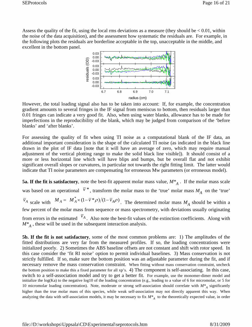
Assess the quality of the fit, using the local rms deviations as a measure (they should be < 0.01, within the noise of the data acquisition), and the assessment how systematic the residuals are. For example, in the following plots the residuals are borderline acceptable in the top, unacceptable in the middle, and excellent in the bottom panel.
However, the total loading signal also has to be taken into account: If, for example, the concentrationgradient amounts to several fringes in the IF signal from meniscus to bottom, then residuals larger than0.01 fringes can indicate a very good fit. Also, when using water blanks, allowance has to be made forimperfections in the reproducibility of the blank, which may be judged from comparison of the ‘before blanks’ and ‘after blanks’.
For assessing the quality of fit when using TI noise as a computational blank of the IF data, anadditional important consideration is the shape of the calculated TI noise (as indicated in the black linedrawn in the plot of IF data [note that it will have an average of zero, which may require manualadjustment of the vertical plotting range to make the solid black line visible]). It should consist of amore or less horizontal line which will have blips and bumps, but be overall flat and not exhibitsignificant overall slopes or curvatures, in particular not towards the right fitting limit. The latter wouldindicate that TI noise parameters are compensating for erroneous Mw parameters (or erroneous model).
5a. If the fit is satisfactory, note the best-fit apparent molar mass value, M*A . If the molar mass scale
was based on an operational , transform the molar mass to the ‘true’ molar mass MA on the ‘true’
scale with . The determined molar mass MA should be within a few percent of the molar mass from sequence or mass spectrometry, with deviations usually originating
from errors in the estimated . Also note the best-fit values of the extinction coefficients. Along with M*A , these will be used in the subsequent interaction analysis.
5b. If the fit is not satisfactory, some of the most common problems are: 1) The amplitudes of thefitted distributions are very far from the measured profiles. If so, the loading concentrations wereinitialized poorly. 2) Sometimes the ABS baseline offsets are not constant and shift with rotor speed. Inthis case consider the ‘fit RI noise’ option to permit individual baselines. 3) Mass conservation is not strictly fulfilled. If so, make sure the bottom position was an adjustable parameter during the fit, and ifnecessary remove the mass conservation constraint. When fitting without mass conservation constraint, uncheck the bottom position to make this a fixed parameter for all xp’s. 4) The component is self-associating. In this case, switch to a self-association model and try to get a better fit. For example, use the monomer-dimer model and initialize the log(Ka) to the negative log10 of the loading concentration (e.g., leading to a value of 6 for micromolar, or 5 for10 micromolar loading concentration). Note, moderate or strong self-association should correlate with M*A significantly higher than the true molar mass of this species, while weak self-association may not directly apparent this way. When analyzing the data with self-association models, it may be necessary to fix M*A to the theoretically expected value, in order
to avoid strong correlation of the Mw and log(Ka) parameters. In case of self-association, the experiment should be repeated with several loading concentrations of this component. Also, self-association, if unexpected, should be reconciled with separate sedimentation velocity experiments, where it should show in the form of a concentration-dependent weight-average s-value. This will help to discriminate the self-association model, and to distinguish self-association from the presence of impurities. 5) Impurities of small molar mass or aggregates are present; inspect SDS-PAGE, HPLC elution profiles, or c(s) SV distributions of the recovered sample. Sometimes, impurities will exhibit significantly different signals at particular wavelengths: for example, contaminations with peptides containing no aromaticamino acids will show strongly at 230 nm, not at all at 280 nm, and very little in IF – in this case, it can be advantageous to exclude the 230 nm data from consideration. 6) Thermodynamic non-ideality is affecting the sedimentation at high concentration; this will generate a distinctly lower slope of the profiles than predicted by the fittedlines at higher concentrations.
6. Repeat Steps IV.2 – IV.5 with the second component. Use the same as an operational quantity, and derive the apparent molar mass M*B of the second component based on the same scale as with the first component. In this way, although the apparent molar mass values appear differentthan the known sequence molar mass, they are valid for the interpretation of the centrifugationexperiment on the particular scale, and they are directly additive in complex formation, for example, M*AB = M*A+M*B.
Determining the equilibrium binding constant of the hetero-association
7. Load the data. For each cell with mixtures, assemble the scans at each wavelength (and IF) intoSEDPHAT configurations as described above in Step IV.2. Set the meniscus, bottom and fitting limits as before in Step IV.2. Mark the bottom position to be a floating parameter, and link different xp’s from the same cell but different ABS wavelength to have the same meniscus and bottom. Use the sameoperational and enter the predetermined extinction coefficients for the respective wavelength(unmarked as fixed parameters). Save the Configuration (use the ‘copy all data and save as new config’function).
8. Set up the parameters. Select the ‘A + B AB Hetero-Association’ model. Load xp files of all mixtures in SEDPHAT. Not all wavelengths are absolutely required, but the loaded set should containthe most informative signals (usually 230 nm for the lower concentrations, 250 nm for the highestconcentrations). If possible, IF data should be combined with at least one ABS signal from the samecell.
In the global experiment parameters, enter the predetermined values of the apparent molar masses foreach component, M*A and M*B. Mark the ‘atot’ and ‘btot’ field to optimize the local concentrations in each cell. Switch the mass conservation model on. Set the log(Ka) field to an expected value (forexample, – 5 for binding constant of KD = 10 micromolar). Uncheck the s-values for all parameters. Set the incompetent fractions to zero in the ‘incfA’ and ‘incfB’ fields, and uncheck these fields. Uncheck ‘add non-participating species’. Check ‘Mass Conservation’, if mass conservation constraint could be applied for both analyses of the individual components A and B. (But even if the mass conservation is not fulfilled for A and/or B, it is advisable to use mass conservation as an approximation in a first stage of the fit, i.e. to getthe concentration and other parameters in a good range, and then in a second stage of the fit to eliminate the massconservation constraint.)
Dependent on the choice of the titration or dilution series for the mixtures in Step I.5, in the global
parameters either toggle to the ‘both A,B in micromolar concentration’ field, or to the ‘A in micromolar conc and B/A molar ratio’ field. The former is advantageous for titration series, because it allows to use the constraint of a constant concentration in A (or B) among the data of different cells, while the latter isadvantageous for dilution series, because it allows to constrain the molar concentration ratio to remainconstant among different cells of this dilution series. (Even though it is very difficult to know exactlythe molar ratio, it is certain that the molar ratio remains constant in a dilution series.) These constrainsare extremely useful to eliminate the correlation between the estimate of the binding constant and theratio of the loading concentrations, which exists for interactions between proteins which are too similar(M*B < 2×M*A or M*A < 2×M*B) or too dissimilar (M*B > 10×M*A or M*A > 10×M*B) in size.
In the local parameters, for each cell enter the loading concentrations of both components (inmicromolar units), or component A (in micromolar units) and the ratio B/A (molar ratio), respectively. In doing so, establish links redirecting the loading concentrations for data sets of different signals fromthe same cell to point to only one ‘experiment’ (or ‘xp’ data channel) for each cell, and establish links that reflect the titration or dilution configuration among the cells (for example, in a titration series withconstant A by redirecting the concentration parameter of A of all cells to that of xp #1) .
Update the configuration (including xp’s).
9. Fitting. Use the ‘Run’ command to verify that the initial estimates of the parameter values producetheoretical distributions in the correct order of magnitude. If the solid lines indicating the theoreticalmodel do not at least appear in the same plot following the same general trends as the data, double-check that the correct extinction coefficients are used in each xp, and manually explore differentconcentration values. When it is difficult to get reasonable starting conditions, sometimes the following strategy helps: Set the bottom values for all cells to a graphically determined value (or 7.2 cm for double-sector cells), and uncheck this parameter in all xp parameter boxes. Also, uncheck the log(Ka) in the global parameter box, such that the concentrationvalues are the only unknowns to be fitted. For samples with equimolar loading concentration, set the B/A molar ratio to 1and fix this value. Then use the Fit command to ‘pre-optimize’ the concentrations and get them in the right ballpark. After that, revert back to the floating log(Ka) and floating bottom parameters. Also, if applicable, revert back to a floating B/Amolar ratio (since the precise molar ratio usually cannot be known accurately enough a priori to serve as a fix constraint).
Fit the model (execute the fit command) with alternating optimization methods (to be switched in theOptions Fitting Options menu). The simulated annealing method is particularly powerful to findglobal minima, since the error surfaces of sedimentation equilibrium models for interacting systemstypically exhibit shallow local minima that can be difficult to deal with. After parameter values haveconverged, and no improvement can be found with either optimization method, save (update) theconfiguration and document the result. Assess the quality of the fit, using the criteria outlined above inStep IV.4.
If the fit is not acceptable, there are several possible explanations: (1) A possible consideration is oftenthe existence of a subpopulation of material incompetent to associate. (This can be tested by including‘incfA’ and/or ‘incfB’ as floating global parameters. But critically inspect the returned values after fitting: A value of 0.5, for example, means that 50% of material was binding incompetent – a number that may be ruled out based on other knowledge on the protein, such as mobility shift or gel filtration data. In contrast, a value of 0.05 would indicate 5%incompetent material, which is hard to rule out by any method.). (2) In rare cases, mass conservation may not befulfilled for the mixtures, even though it is fulfilled for each individual component. To test this, switchoff mass conservation (see the additional comments in Step IV.5.b). (3) The sample may be contaminated with a contaminating species not participating in the binding reaction. This can beassessed from accompanying SV experiments, where c(s) can provide Mw estimates for this component,if the mass is outside the range of those of the individual components and the complexes. This speciescan be accounted for in the SE data analysis here using the ‘add non-participating species’ option. Note
that the loading signal (directly in signal units) for this species in each xp will need to be initialized, andshould be floated. (4) Alternatively, different association models may be explored. For example, if thetheoretical lines are systematically not steep enough compared to the data in the region close to the rightfitting limit, and if this mismatch increases with higher loading concentrations, an association modelwith larger complex is indicated.
10. Inspect the reliability of the fit in three ways: (1) If TI noise was used to calculate a baseline blank in either IF or ABS data, verify that it does not show significant overall slopes and curvaturestowards the right fitting limit. If this is the case, there is a correlation between fitting the concentrationgradients and the baseline, and the TI noise calculated blank should be switched off. (2) Visualize thecontributions of the complex to the signal. This will reveal whether for the given experimentalconcentration range and the calculated KD any significant complex formation is predicted: If not, then the KD value certainly cannot be determined from the given data, and only a lower limit can becalculated. Vice versa, visualize the contributions of the free components – if they are essentially zero, i.e. if any one is not predicted to contribute significantly to the signal, then binding cannot bedistinguished from stoichiometric binding and only an upper limit for the KD can be extracted from thedata. The respective traces for these species can be switched on in the Display menu.
11. Perform a statistical error analysis on the determined binding constant. Different methods are available in SEDPHAT, but the most reliable and most rigorous approach is the projections of the errorsurface method (Bevington and Robinson 1992). (For ‘simple’ fits, the Monte-Carlo approach works well.) Although the absolute value of χ2 (‘global red. chi-square’ in SEDPHAT) should not be interpreted without absolute knowledge on the noise in the data, the relative increase of χ2 comparing the original and the new fit is a statistical quantity that can be evaluated using the F-statistics. Calculate the critical value for χ2 (with the SEDPHAT statistics function). Set the value of the binding constant ata non-optimal value close to the best-fit parameter (for example, increase log(KA) by 0.05), fix the binding constant but float all other unknown parameters in a new fit. If the original fit was the best fit,then the current fit will have a higher χ2. If the new value exceeds the critical value, then the modified binding constant is outside of the error interval. If it is less than the critical value, fix log(KA) at a value a little bit further from the best-fit value and re-fit. Repeat this until the critical χ2 is exceeded, which indicates that one of the limits of the log(KA) error interval has been found. Reload the best-fit configuration and repeat the procedure by changing log(KA) in the other direction. An illustration of this approach can be found in (Schuck et al, 1999).
Appendix: Test approach to equilibrium
(SEDFIT version 10.11, April 2007 or newer).
1. Load all scans collected thus far (by either absorbance optics or interference detection, not both) in anew SEDFIT window.
2. Set upper and lower “fitting” limits. The lower limit should be to the right of the meniscus and the
bottom fitting limit should be located at a position where the signal is linearly dependent onconcentration. Optical artifacts must be excluded from the range between the fitting limits.
3. Reveal the drop-down menu under the loading options item of the Options tab and select “test for approach to equilibrium”.
4. Indicate whether the indicated scan (cell x, speed j) should be included in the plot of the ‘time-course to equilibrium’. This scan could be omitted for example if it appears that it will not be useful for data analysis perhaps because the signal is too low or there is insufficient curvature.
5. “Accept radial limits for comparison…” answer ‘Yes’ to this question if the limits (indicated by the red line overlaying raw data) are acceptable. Answer ‘No’ if the limits need to be adjusted.
6. Continue in this manner for the remaining scans at available rotor speeds.
7. “Real time update?” Answer ‘Yes’ if you would like the software to automatically update the ‘time-course to equilibrium’ plot with new scans that acquired at later times and rotor speeds. The user may choose whether to use the default limits already set previously for the additional scans loaded in the real-time update. The user may also choose whether to include scans that are acquired later for cells that hadnot yet been included in the time-course plot.
Appendix: SEDFIT function “Sort EQ Data to Disk”
(SEDFIT version 10.11, April 2007 or newer). For screenshots of this function, see http://www.analyticalultracentrifugation.com/eqtest.htm.
1. Load all scans (from all cells, rotor speeds, and wavelengths) collected by either interference or absorbance detection (but not both types at once).
2. With the left mouse button, double-click (and then hit ENTER) to set up initial positions for the upper and lower radial fitting limits. The fitting limits should span the entire range of radii that willlikely be included for data analysis (linear concentration range) and excluding the regions containingoptical artifacts near the meniscus and cell bottom. They will be refined later.
3. From the “Loading Options” menu under the “Options” tab, select “Sort Equilibrium Data to Disk”, point to where the data should be saved (it is recommend that the data be saved in a folder entitled“SortedEQData”). Choose not to “Subtract Blank File” (as this option only allows to select a single blank file, which is not sufficient when handling data from different cells and/or rotor speeds). Acceptthe option to “make XP Files” – this will result in the creation of a multi-speed equilibrium file comprised of the final scan at each rotor speed for a particular signal. Input buffer density, proteinpartial specific volume and molar extinction coefficients or accept default values (these can be changedlater) into the resulting dialog boxes. A plot will appear that shows the root-mean-square difference in signal between each scan and the latest respective scan acquired and a dialog box inquiring whether thesample had reached sedimentation equilibrium. For this judgment, see also the comments in Step III.8
above. Selection of “yes” will generate a data file comprised of the last scan at the indicated speed andwavelength. A new dialog box will appear inquiring whether to include that data set in a multi-speed equilibrium xp file.
4. Continue responding to the remaining dialog boxes indicating whether a particular cell attained sedimentation equilibrium at each indicated rotor speed and input signal, and whether to include thefinal scan in a multi-speed equilibrium xp-file.
References:
J. Vistica, J. Dam, A. Balbo, E. Yikilmaz, R.A. Mariuzza, T.A. Rouault, P. Schuck (2004) Sedimentation equilibrium analysis of protein interactions with global implicit mass conservation constraints and systematic noise decomposition. Analytical Biochemistry 326:234-256 P. Schuck and D. Millar (1998) Rapid determination of molar mass in modified Archibald experiments using direct fitting of the Lamm equation. Anal. Biochem. 259:48-53 P.R. Bevington an D.K. Robinson. Data Reduction and Error Analysis for the Physical Sciences. McGraw-Hill, New York, 1992 P. Schuck, C.G. Radu, and E.S. Ward (1999) Sedimentation equilibrium analysis of recombinant mouse FcRn with murine IgG1 and Fc fragment. Mol. Immunol. 36:1117-1125


![Experimental Investigation of Ba e E ect on the Flow in a ...scientiairanica.sharif.edu/article_3326_457545225e84e1ee2ed6f636… · Schroeder [15] on primary sedimentation tanks showed](https://static.documents.pub/doc/80x56/5fbb48f3fc31be42595e6bc9/experimental-investigation-of-ba-e-e-ect-on-the-flow-in-a-schroeder-15-on.jpg)

