Exploratory Analysis of Anchoveta Recruitment off Peru and Related Environmental Series* ROY MENDELSOHN PacificFisheries EnvironmentGroup Southwest FisheriesCenter P.O. Box 831 Monterey, California 93942 USA JAIME MENDO Instituto del Mar del Peru Apartado22, Callao, Peru MENDELSOHN, R. and J. MENDO. 1987. Exploratory analysis of anchoveta recruitment off Peru and related environmental series, p. 294-306. In D. Pauly and L Tsukayama (eds.) The Peruvian anchoveta and its upwelling ecosystem: three decades of change. ICLARM Studies and Reviews 15,351 p. Instituto del Mar del Peru (IMARPE), Callao, Peru; Deutsche Gesellschaft flIr Technische Zusammenarbeit (GTZ), GmbH, Eschbom, Federal Republic of Germany; and International Center for Living Aquatic Resources Management (ICLARM), Manila, Philippines. Abstract An exploratory analyzis of monthly anchoveta (Engraulis ringens) recruitment estimates and associated biological and environmental series for thn years 1953 to 1981 was performed with the aim of investigating the possibility of forecasting anchoveta recruitment three months ahead of tb .e. While the high degree of autocorrelation in the monthly recruitment serier prevented the identification of ciusal models, yearly models combining pairs of adjacent months were identified which appear promising as a means to forecast future trends in anchoveta recruitment. These models, however, do not appear to conform to any of the conventional hypotheses providing mechanisms to explain recruitment fluctuations. Introduction Recruitment is one of the most important but least understood components of fish population dynamics. Several authors have tried to empirically relate larval survivorship with environmental parameters (Bailey 1981; Lasker 1981). These efforts to relate recruitment variability with environmental variability have not been notably successful due to the very short data series generally available for empirical analysis (Bakun 1986). Major recent studies have indicated environmental-biological linkages for pelagic and demersal species of the California Current, Canary Current and Guinea Current (see Bakun 1986). Wind induced Ekman transport, a turbulent mixing index (wind speed cubed) and temperature also have been used in several studies of environmental effects on fish stocks (e.g., Collins and MacCall 1977; MacCall 1980; Bakun and Parrish 1980; Mendelsohn and Cury 1987). Similar studies have yet to be done for the Peruvian anchoveta (Engraulis ringens) which in the early 1970s generated the highest catch of any single-species fishery in the world (Tsukayama and Palomares, this vol.; Castillo and Mendo, this vol.), and whose biomass was well over 20 t x 106 by the end of the 1960s (Pauly, Palomares and Gayanilo, this vol.). The collapse of the anchoveta fishery has been attributed both to overfishing and to the influence of El Niflo which may have changed the usual spawning patterns of the anchoveta (Santander 1980). *PROCOPA Contribution No. 53. 294
Transcript
Exploratory Analysis of Anchoveta Recruitment off Peru and Related Environmental Series*
MENDELSOHN, R. and J.MENDO. 1987. Exploratory analysis of anchoveta recruitment off Peru and related environmental series, p. 294-306.In D. Pauly and L Tsukayama (eds.) The Peruvian anchoveta and its upwelling ecosystem: three decades of change. ICLARM Studiesand Reviews 15,351 p. Instituto del Mar del Peru (IMARPE), Callao, Peru; Deutsche Gesellschaft flIr Technische Zusammenarbeit(GTZ), GmbH, Eschbom, Federal Republic of Germany; and International Center for Living Aquatic Resources Management(ICLARM), Manila, Philippines.
Abstract An exploratory analyzis of monthly anchoveta (Engraulis ringens) recruitment estimates and associated biological and environmentalseries for thn years 1953 to 1981 was performed with the aim of investigating the possibility of forecasting anchoveta recruitment three monthsahead of tb .e.While the high degree of autocorrelation in the monthly recruitment serier prevented the identification of ciusal models, yearlymodels combining pairs of adjacent months were identified which appear promising as a means to forecast future trends in anchoveta recruitment.These models, however, do not appear to conform to any of the conventional hypotheses providing mechanisms to explain recruitment
fluctuations.
Introduction
Recruitment is one of the most important but least understood components of fishpopulation dynamics. Several authors have tried to empirically relate larval survivorship withenvironmental parameters (Bailey 1981; Lasker 1981). These efforts to relate recruitmentvariability with environmental variability have not been notably successful due to the very shortdata series generally available for empirical analysis (Bakun 1986). Major recent studies haveindicated environmental-biological linkages for pelagic and demersal species of the CaliforniaCurrent, Canary Current and Guinea Current (see Bakun 1986). Wind induced Ekman transport,a turbulent mixing index (wind speed cubed) and temperature also have been used in severalstudies of environmental effects on fish stocks (e.g., Collins and MacCall 1977; MacCall 1980;Bakun and Parrish 1980; Mendelsohn and Cury 1987).
Similar studies have yet to be done for the Peruvian anchoveta (Engraulisringens)which inthe early 1970s generated the highest catch of any single-species fishery in the world(Tsukayama and Palomares, this vol.; Castillo and Mendo, this vol.), and whose biomass waswell over 20 t x 106 by the end of the 1960s (Pauly, Palomares and Gayanilo, this vol.). Thecollapse of the anchoveta fishery has been attributed both to overfishing and to the influence ofEl Niflo which may have changed the usual spawning patterns of the anchoveta (Santander1980).
*PROCOPA Contribution No. 53.
294
295
The biology of the anchoveta is rather well documented (see relevant contributions in this vol.). Spawning in anchoveta tends to have two peaks per year - one in the austral winter-springand the other in austral summer. The major spawning concentrations usually occur near the coast up to around 105 km offshore. Since the 1960s, the Instituto del Mar del Peru (IMARPE) has carried out anchoveta egg and larval surveys (see Santander, this vol.), but these data do notnecessarily indicate variations in anchoveta recruitment due to density-dependent eggcannibalism, otir sources of egg mortality and fluctuations in survival of the larvae (see Pauly,this vol.).
Several authors (Santander 1980; Mendiola and Ochoa 1980; Tsukayama and Alvarez 1980;Santander and Flores 1983) have presented evidence showing that during El Niffo years, primaryproductivity decreased and the periods of peak spawning changed resulting in lower recruitment. These two factors have been thought to be the major environmental influences on recruitment variability.
In this paper we perform an exploratory data analysis of the estimated recruitment and biomass series of Pauly, Palomares and Gayanilo (this vol.), of the egg production series inPauly and Soriano (this vol.) and of several of the various environmental series gathered in thisvolume. Our interest is in determining if it is possible to forecast anchoveta recruitment at least three months ahead of time, a forecast that would be useful in managing the fishery.
Exploratory data analysis has the advantage in this situation where little is known in that we do not try to force the data into models that may not agree with the structure of the observed data. Despite the variety of fisheries models available, there is no "physics of fisheries" in the sense of known laws that have been experimentally verified. Letting the data lead us to a model structure leaves us open to alternative causal explanations as well as providing a check on the realism of the estimated series, identifying outliers in the data and flagging data points that maybe overly influential in the analysis.
The Data
The anchoveta population data used are the estimates presented by Pauly, Palomares and Gayanilo (this vol.). The environmental series consisted of sea surface temperature (SST) and oceanic wind speed cubed and offshore transport derived by Bakun (this vol.), as well as hourlywind direction and intensity recorded at Trujillo and Callao airports by CORPAC (CorporacionPeruana de Aviacion Comercial). The Trujillo and Callao data are described further in Mendo et al. (1987) and Mendo et al. (this vol.).
Offshore transport at both Trujillo and Callao were calculated as in Bakun (1973 and this vol.), as was wind speed cubed for both locations. Peterman and Bradford (1987) report using anindex reflecting Lasker's hypothesis (1978) to predict the survival of anchovy Engraulismordax larvae off California. A similar index was computed for both Trujillo and Callao; it measures the number of 4-day periods during which the wind speed did not exceed 5m/sec. These 4-dayperiods are here called "Lasker events", as suggested by D. Pauly (pers. comm.).
Spectral analysis showed that the Trujillo and Callao wind series were not significantlycoherent at all frequencies. The Trujillo wind series were only coherent with the oceanic wind series at a frequency of 6 months (though out of phase) and at frequencies longer than a year.The oceanic series show a pronounced seasonal cycle, the Callao series a smaller seasonal cycleand the Trujillo series showed essentially no seasonal cycle. The general impression is of stronglocal differences suggesting the need for care in choosing what variables to use in the analysis.
The Lasker events were problematic at best. At Callao, the wind always satisfied the criteria, while at Trujillo most months had a zero incidence of the necessary periods of calm,especially during 1955-1970, when recruitment was at high levels (see below and Table 1). The estimated recruitment following the periods of zero counts vary grealy, making Lasker events of little use for these periods. For the periods where numerous Lasker events occurred, examination of the data revealed that a high number of events tended to precede low rather than highrecruitment. Lasker's hypothesis is based on experience in California where turbulence dispersesthe food necessary for larval survival; in Peru the food concentration in the mixed layer may be
296
high enough for turbulence not to have that great an effect. All that can be said with certaintyfrom this is that the situation in Peru appears to differ from that in California.
Table 1. Monthly occurrence of "Lasker events" near Trujillo, 195 3 .19 85 .a
Year Jan Feb Mar Apr May Jun Jul Aug Sep Oct Nov Dec
abased on data in Mendo et al. (1987); a "Lasker event" is a period of calm (wind speed below 5 m/s) lasting 4 days; periods of 5 days are viewed as two partli overlapping 4-day events, etc. (see Peterman and Bradford 1987, note 16).
Based on this preliminary analysis of the environmental series, we restricted our attention to the wind variables at Trujillo. The Trujillo station has no nearby topographic interference, such as mountains, and the coastline from one degree north of Trujillo to one degree south of Trujillois almost straight. The area off Trujillo also is one of the major anchoveta spawning areas (Santander and Castillo 1973; Santander 1980, this vol.).Localized trends were calculated using the "lowess" algorithm of Cleveland (1979) for recruitment, egg and total biomass as well a- for offshore transport and wind speed cubee! atTrujillo. Both the recruitment and total biomass series exhibit three periods with distinct :+neanlevels. A pre-1960 period with low levels of biomass and recruitment, a period from 1960 to1972 when both biomass and recruitment were at high levels, and a post-1972 period foil awingthe collapse of the fishery (see Pauly, Palomares and Gayanilo, this vol.). On a log scale, for the1960-1972 period, the trend line for both recruitment and total biomass is almost flat, suggestingrandom variation around a fixed mean level.
297
RecruitmentSeries
For our initial look at anchoveta recruitment we examined the dynamics of the recruitmentseries by decomposing it into three components - localized trend, seasonal and autoregressive(AR) components (Fig. 1), using an algorithm of Gersch and Kitigawa (1983). The variation inrecruitment is dominated by longer-term behavior captured in the estimated trend, as the AR component is an order of magnitude smaller than the recruitment series and the seasonal component is almost two orders of magnitude smaller.
1.2 A 1.2 B 1.0 1.0
06 0.8
0.4 - 0.4
0.2 .__I_1_______
0.2 - /
05 3 55 57 59 61 63 65 67 69 71 73 75 77 79 81 53 55 57 59 61 I I I I I I I I".",4,,63 65 67 69 71 73 75 77 79 81
Fig. 1. Decomposition of the anchoveta recruitment time series into its component parts: (A) observed data; (B) nstimated trend;(C)autoregressive component; (D) seasonal component (see text for details).
The estimated local trend (Fig. IB) suggests three different periods: a low level ofrecruitment from 1953 to 1958, a higher level from 1959 to 1969 or 1970, followed by a sharpdrop in recruitment which preceded:(i) the El Ni-o even to 1972-1973, (ii) the collapse of thefishery, (iii) and by a year, the drop in total biomass. This suggests that the effects of El Niffos onthe population dynamics of anchoveta may be more complex than previously thought. The 1971recruitment collapse must have been due to overfishing or environmental effects the previousyears since the collapse of the fishery appears to have begun before the El Nifio.
The st asonal component (Fig. ID) is very regular but of such small magnitude as to bealmost unnoticeable in the overall variation in recruitment. The autoregressive component (Fig.1C) alsc suggests three periods: a period from 1953 to 1961 of relatively small variations, aperiod from 1961 to 1972 of large variations coinciding with the growth of a large-scale fisheryand a period from 1972 or so onwards following the collapse of the fishery which is also a periodof smaller variations in recruitment. The period of high variability from 1961 to 1972 also is aperiod of high estimated total biomass.
The autocorrelation function of recruitment both on the normal and tie log scale i;s highlynonstationary and dominated by a value of .95 at a lag of one month. A simple model thatincludes an autoregressive term of recruitment on itelf at lags 1,2, 6 and 12 months explainsalmost 96%of the variance in the monthly series. This agrees with the decomposition of the time
298
series: monthly estimates of recruitment have not increased our degrees of freedom as the seriesis not independent at monthly time spans; rather, the important variation is between years.
The high degree of autocorrelation in the monthly recruitment series is probably caused by(i) the fact that the sampled length-frequency data may not be accurate enough to resolve monthly differences in population structure so that the size information tends to be "smeared" across months, (ii) the fact that Virtual Population Analysis (VPA) uses a series of recursive equations that estimate the present biomass levels from the data from successive periods; these equations will tend to smooth the observed data towards low-order autoregressive behavior,reducing the independence of the monthly data and (iii) the fact that the version of lengthstructured VPA used by Pauly, Palomares and Gayanilo (this vol.) increases the inherent tendency of VPA to smooth data across months (D. Pauly, pers. comm.).
There are several approaches for analyzing the recruitment series given this high degree of autocorrelation. We can low-pass filter the series and then decimate the results to one or tworepresentative values a year and use these data points as the new time series. Alternatively, we can form separate annual series of seasonal segments of the annual cycle and fit separate models across years for each of the aggregate series, comparing the results of the different models. This second approach has an added advantage that it allows us to check for time-dependentrelationships in the data. In what follows we restrict ourselves to this second approach.
Bimonthly Recruitment Series
As an initial examination of the data by months across years, we constructed box plots(Velleman and Hoaglin 1981) for each of the series (Fig. 2). A plus marks the median of the data, the I's mark the hinges plus or minus 1.5 times the H-spread, where the hinges are the medians of the two halves of the series defined by the median and the H-spread is the difference between the two hinges. The lines beyond the boxes show the outer normal range of the datawhich is defined as the hinges plus or minus 3 times the H-spread. Values somewhat outside this range are marked with dots and values far outside this range with open dots. Finally, the parentheses denote a confidence limit on the medians.
Recruitment (Fig. 2A) starts ou: in January at a relatively lower level, increases gradually to a recruitment peak around May-July and then slowly decreases to the end of the year. Eggproduction, however, has a relative peak around February-March and a much larger peak around September-October. Parent biomass (Fig. 2C) has a large peak in February-March concurrent with the relative -I'eak in egg production but usually has relatively low value during the September-October period. Thus assuming the recruits to be 3-4 months old (see Palomares et al., this vol.), the larger recruitment in June-July would stem from the lesser spawning ofFebruary-March, which is based on a large parent biomass. Conversely, the lesser r..cruitment in the beginning of the year would stem from the major spawning in September-October, which is based on a relatively small parent biomass. The wind-related environmental series (Figs. 2E and2F) are at a relative minimum during the February-March period, but are at their maxima duringthe September-October period and thus generate unfavorable environmental conditions. Parrish et al. (1984) also comment on the large austral spring spawning during unfavorable conditions. One possible explanation for a large spawning during unfavorable conditions is that the conditions during this period are favorable for the adults (it is the upwelling period). A. Bakun(pers. comm.) has suggested that such a low degree of apparent adaptation of spawning effort to the normal seasonality of larval survival prospects might be in some way due to the fact that detrimental El Niiio effects may exert strongest impact during the warm austral summer period;thus the effects of intermittent reproductive failures during summer, associated with El Ninfo anomalies may have tended to counter adaptive tendencies to concentrate spawning in the normally favorable summer season.
After examination of the recruitment series and the environmental series we decided on bimonthly aggregation of the recruitment series as follows: February-March, April-May, June-July, August-September, October-November and December-January. Note thai the December-Januar aggregate crosses years: December 1953 is combined with January 1954, etc. Thesepairs of months vary across years in a similar manner and at similar levels (Fig. 3). For
299
A IIB I tnhio rcrultt Log(EggProduction) . .
T I:~ ! i IanFlt-orA May A q ep Oct Nov Dec Jon Feb~aI a u u Aug.,SopOct Nov onc
SNSpOcNov Doc Jn Feb r My Jun Jui Au S* Oct Nov
E Trujillo trenspbrtAkne Trujiltwindspeetcubed
41
.++
Jon FebMet AprMay Jun JulAug Sep Oct Nov Dec Jn Feb Mu A Myc m Jul Aug Sep Oct Nov Dec
Fig. 2. Boxplots of the monthly anchoveta and wind-based environmental series: (A) recruitment; (B) log of egg production; (C) parent biomass; (D) total biomass; (E) Trujillo offshore transport; (F) Trujillo wind speed cubed (see text for definition of ordinate and data sources).
predictors we considered parent biomass and egg production lagged 3 and 4 months (thespawning period) as well as the monthly offshore transport and wind speed cubed at Trujillo.Spectral analysis of the transport and wind speed cubed at Trujillo shows that these series arehighly coherent (> .9) at all frequencies and thus have essentially the same dynamics due tolimited variability in the wind direction (Mendo et al., this vol.). We therefore arbitrarily restrict our attention to offshore transport, though similar results can be found using wind speed cubed,i.e., turbulence.
Cross-correlation matrices as well as generalized partial correlations were calculated as inTiao and Box (1982). Model and variable selection were also examined using the multivariatesubset autoregression procedure of Akaike et al. (1979). As it is likely that the relationshipsbetween recruitment and the environment is nonlinear, final model selection and identification was done using the AVAS procedure (Tibshirani 1987). This procedure is a modification of theoptimal transformation algorithm ACE (Breiman aiid Fxredman 1985) which appears to correct
300
1.0 - 4v-0--o FebruaryMarch 0-B April0_ may ! 2
g 0. .it I 08?
I "I0 -A 1955 1960 1965 1970 1975 1980 1955 1960 1965 1970 1975 1980
Fig. 3. Monthly anchoveta recruitment across years, 1953 to 1981: (A) February-March; (B) April-May; (C) June-July; (D) August-September; (E) October-November; (F) December-January.
some of the problems with that algorithm, by restricting the transformation of the dependent vaiable to be monotone and variance stabilizing (Efron 1982).
Both the approach of Tiao and Box (1982) and the subset autoregression procedure suggested the same behavior in all the series. Each of the bimonthly recruitment series had a significant relationship with recruitment two years hence. Parent biomass 3 and 4 months earlier appears to have no significant effect on recruitment. Except in one case to be discussed below, environmental conditions during the spawnhig period also do not appear to be strongly related to recruitment. Egg production was not examined for all the bimonthly series; however, for the models in which egg production was used as a variable it also was not significantly related to recruitment 3-4 months later.
For all six bimonthly series, offshore transport during the austral spring period September-November was identified as the important predictoi of recruitment, and that the strongestrelationship appeared to be with September transport. To obtain our models, the AVAS algorithm was used on each of the six bimonthly recruitment series, using recruitment two years earlier and September-November transport as variables. The variables were selected in a stepwise fashion by first identifying the best single variable, then by finding the second variable that when added to best single predictor produces the most increase in r-square value, etc. As a partial check on our procedure, mon ly transpo;r series were chosen at random for inclusion in our analysis; at no point did any of these series produce a significant result. Since AVAS produces transformations that can improve the relationship between variables if the relationship is nonlinear, we also tested the inclusion of parent biomass and environmental conditions 3-4
301
months previous to recruitment. Again, with one exception, none of these series added significantly to our results.
The models estimated by AVAS all had estimated r-square values in the range of .75 to .80. Given the relative short length of our time series as well as the amount of searching we did overvariables, it would not surprise us if this value is inflated as a measure of prediction r-square,that is of expected error in forecasting future data rather than the error from the data used to estimate the models (see also Efron 1986; Hastie and Tibshirani 1986). AVAS findsrelationships by using smoothers to estimate condition expectations, and the parameters for thesesmoothers are chosen using generalized cross-validation which at least asymptotically shouldreflect prediction error (Friedman and Stuetzle 1982; Breiman and Friedman 1985; Hastie andTibshirani 1986). Also, as we discuss below, the models tend to fit the series by measures other than r-square, particularly in anticipating turning points in the series.
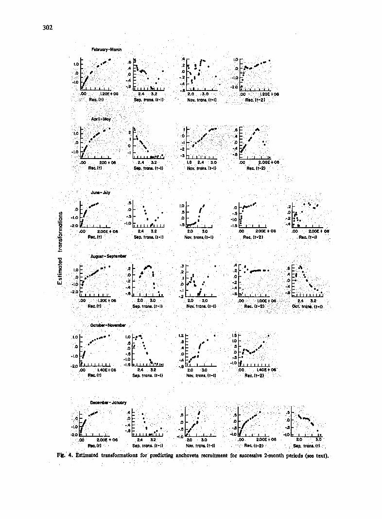
The estimated transformations (Fig. 4) are similar for each of the six models for all variables. (AVAS calculates empirical transformations so the form of the transformation isdetermined by plotting the transformed variable against the original variable. All transformations are standardized to have zero mean and variance of 1; this is necessary for identification of thetransformations.) Recruitment at time t is transformed to a form very close to a logtransformation. This agrees with our observation of the decomposed recruitment series that theseries appears to have increased variance at higher levels; the log transformation stabilizes thevariance in this instance. A log transformation also means that environmental effects are on aproportional rather than an absolute basis, which, apriori,appears to be more sensible.
The estimated transformation for recruitment at time t-2 suggests two separate regimes -periods of relatively lower recruitment and periods of higher recruitment. The transformations suggest that the behavior is almost like an indicator function - the group, rather than the exactlevel, being the important information. At first glance, a 2-year lag in recruitment would seem toreflect the effect recruitment has on the spawning biomass for the recruits at the present timeperiod. Howev, r, as previously mentioned, parent biomass during the spawning period is not a good predictor and adds little to our model. The mechanistic interpretation of the 2-year lag in recruitment therefore is an open question.
The transformation of transport during the previous September generally increases to a peakat around a value of 2.5, which corresponds to a wind speed of roughly 6 m/sec, decreases to aminimum with a value of 3, roughly corresponding to a wind speed of 7 m/sec and then increasesagain. Note that wind speeds between 6 and 7 m/sec correspond to the transitional level at which water changes from being hydrodynamically "smooth" to being hydrodynamically "rough"(Deacon and Webb 1962).
The transformation of transport in November generally increases, but behaves differentlybetween the same values of 2.5-3. The model appears to be contrasting the September andNovember conditions. Optimal conditions occur when there is some transport in Septemberfollowed by a high level of offshore transport in November. Again, the mechanistic interpretation of these variables is not clear.
The model for December-January recruitment also contains a term for September transportthree months earlier, corresponding to the spawning period. The estimated transformation decreases monotonically, with a particularly sharper slope as wi. idspeed exceeds the 6-7 m/secrange. This term appears to explain why the large egg production during the August throughOctober period does not produce a large number of recruits: egg and larval mortality may bemuch higher. It is interesting that this is the only period dit-ing where conditions duringspawning are important to the model.
On the whole, the model predictions (Figs. 5, 6 and 7) of transformed recruitment appear tobe quite satisfactory. As the estimated transtormations are close to being log transformations, thevalues are similar to taking the log of recruitment and then standardizing the variables. This will not change relative peaks and troughs and trends in the data. As is clear from both the fits and the residuals, none of the models do a very good job for the first five years, 1955-1959. Afterthat, the models appear to track the major turning points quite well, in particular by anticipatingthe major decline in recruitment during the 1969-1971 period and the subsequent increase inrecruitment later on in the 1970s. Apart from the first five years, the residuals are fairly well behaved except for the April-May residuals which show a definite trend throughout the model
Fig. 7. Observed and predicted October-November (A)and December-January (B)anchoveta recruitments, with residuals (C,D).
period. The June-July and August-September models, when recruitment appears to be at or near a maximum, appear to anticipate changes in recruitment quite well.
The biomasses and the recruitment estimates for the period 1953 to 1959 were obtained through VPA using values of residual natural mortality (Mo) which could not be calibrated against independent biomass estimates; moreover, during this period, a large proportion of the withdrawals used for the VPA were estimates of anchoveta consumption by birds and bonito (see Pauly, Palomares and Gayanilo, this vol.). These appear to be sufficient reasons for differences between this period and the succeeding ones and thus cxplain why, in terms of our models, recruitment during this time period behaved in a manner different from the rest of the model period (see also Pauly, this vol.).
Discussion and Conclusions
We have shown that while the high degree of autocorrelation in the monthly recruitment data makes it difficult to identify causal models of anchoveta recruitment, we could, however, identify yearly models for bimonthly recruitment series. These models tend to have a similar structure, predict recruitment with approximately equal success and appear promising as a means to forecast future trends in anchoveta recruitment.
The pattern of the cross and partial correlation matrices, as well as several different modelling approaches, have all suggested the same basic models. Thus we feel confident that the relationships described in our models reflect the basic structure of the data. However, there is no clear biological interpretation of this structure. As we have done an extensive amount of searching through different sets of variables and estimating transform,,'ons to increase model fit, it is likely that our estimates of the goodness of fit of our models and of the ability of the models to predict future data is somewhat inflated. We would therefore recommend to implement the following steps before attempting to implement a model similar to the one analyzed here:
305
(1)Attempt to calibrate the estimated recruitment series with independent data (i.e., data notused in obtaining the estimates) to further verify that the estimated recruitment reflects the actual changes in recruitment, at least on a yearly basis;
(ii) Calculate offshore transport and wind speed cubed from other stations near Trujillo to check on the accuracy and consistency of this data set;
(iii) Develop a better mechanistic understanding of the underlying models. We are distrustful of forecasting models that do not have a clear biological interpretation and for whichthere is no independent evidence for the relationships developed in the exploratory analysis;
(iv) For log recruitment, use techniques that estimate transformations without transformingthe dependent variable, and that allow for greater testing of model parameters, such as GAIM(Hastie and Tibshirani 1986); and finally
(v) Use generalized cross-validation or related techniques to test the stability of both thetransformations and the degree of fit of the models, in order to get a better idea of the predictivecapability of the models for data to be obtained in the future.
Despite these reservations, we feel we have shown that the series of recruitment estimatesproduced by Pauly, Palomares and Gayanilo (this vol.) have properties which enable them toforecast far enough in advance for consideration in the formulation of management actions.Further, we have indicated the impc.-tance of including variables that reflect environmental processes. However, the fact that the resulting models do not appear to conform to any of theconventional hypotheses concerning major influences on recruitment success remains unsettling.
Acknowledgements
This research was made possible through a cooperative agreement between the IMARPEPROCOPA-ICLARM Project and the Pacific Fisheries Environmental Group, SouthwestFisheries Center. In particular we thank Dr. H. Salzwedel, PROCOPA Project Leader and Dr.Schmidt of GTZ for their support of the second author's stay in Monterey. We thank Dr. R.Villanueva, Executive Director of IMARPE, and Dr. Izadore Barrett, Director, SouthwestFisheries Center for allowing this cooperative effort. We also thank Dr. Daniel Pauly ofICLARM, Drs. A. Bakun and R. Parrish and our colleagues at IMARPE and PFEG for comments and support during the completion of this work. Prof. R. Tibshirani kindly provided us with a copy of the AVAS program and answered many questions about its use.
References
Akaike, H., 0. Kitagawa, E. Arahata and F. Tada. 1979. TIMSAC-78, Computer Science Monographs. The Institute of Statistical Mathematics, Tokyo. 11.279 p.
Bailey, K. M. 1981. Larval transport and recruitment of Pacific hake Merlucciusproductus. Mar. Ecol. Prog. Ser. 6:1-9.Bakun, A. 1973. Coastal upwelling indices, west coast of North America, 1946-71. U.S. Dep. Cornmer., NOAA Tech. Rep.
NMFS SSRF-671. 103 p.Bakun, A. 1986. Comparative studies and the recruitment problem: searching for generalizations. CalCOFI Rep. 26:30-40Bakun. A. and R.H. Parrish. 1980. Environmental inputs to fishery population models for eastern boundary current regions, p. 67
104. In G.D. Sharp (ed.) Workshop on the Effects of Environmental Variation on the Survival of Larval Pelagic Fishes,Lima, Peru, April-May 1980. IOC Workshop Rep. 28. Unesco, Paris.
Breiman, L. and J.H. Friedman. 1985. Estimating optimal transformations for multiple regression and correlation. J. Amer. Stat. Assoc. 80:580-619.
Cleveland, W.S. 1979. Robust locally weighted regression and smoothing scatterplots. J. Amer. Stat. Assoc. 74:829-836. Collins, R.A. and A.D. MacCall. 1977. The California Pacific bonito resource, its status and management. Calif. Dept. Fish and
Game, Mar. Res. Tech. Rep. 35.39 p.Deacon, EL. and E.K. Webb. 1962. Small-scale interactions, Chapter 3. In M.N. Hill (ed.) The sea: ideas and observations on
progress in the study of the seas. Interscience, New York. Efron, B. 1982. Transformation theory: How normal is a family of distributions? Ann. Stat. 10:323-339.Efron,B. 1986. How biased is the apparent error rate of a prediction rule? J. Amer. Stat. Assoc. 81:461-471. Friedinan, J.H. and W. Stuetzle. 1982. Smoothing of scatterplots. Tech. Rept. Orion 3, Dept. of Statistics, Stanford University.Gersch, W. and G. Kitigawa. 1983. The prediction of time series with trends and seasonalities. J. Bus. Econ. Stat. 3:253-264. Hastie, T. and R. Tibshirani. 1986. Generalized additive models. Statistical Science 1:297-318. Lasker, R. 1978. The relation between oceanographic conditions and larval anchovy food in the California Current: identification
of factors contributing to recruitment failure. Rapp. P.-V. R~m. Cons. Int. Explor. Mer 173:212-230.
306
Lasker, R. 1981. Factors contributing to variable recruitment of the northern anchovy (Engrauisringens)in the California Current: contrasting years, 1975 through 1978. In R. Lasker and K. Sherman (eds.) The early life history of fish: recent studies. The second ICES Symposium, Woods Hole, Mass., April 1979. Rspp. P.-V. R~un. Cons. Int. Explor. Mer 178:375-378.
MacCall, A.D. 1980. The consequences o" cannibalism in the stock-recruitment relationship of planktivorous pelagic fishes such as Engraulis,p. 201-220. In G.Sharp (ed.) Workshop on th,; Effects of Environmental Variation on the Survival of Larval Pelagic Fishes, Lima, Peru. April-May 1980. IOC Workshop Rep. 28. Unesco, Paris.
Mendelsohn, R. and P. Cury. 1987. Fluctuations of a fortnightly abundance index of the Ivoirian coastal pelagic species and associated environmental conditions. Can. 1.Fish. Aquat. Sci. 44:408-421
Mendiola, B.R. and N. Ochoa. 1980. Phytoplankton and spawning of anchoveta, p. 242-253. In G.D. Sharp (ed.) Workshop on the Effects of Environmental Variation on the Survival of Larval Pelagic Fishes, Lima, Peru, April-May 1980. IOC Workshop Rep. 28. Unesco, Paris.
Mendo, J., L. Pizarro and R.Huaytalla. 1987. Peporte de datos sobre indices de afloramiento y turbulencia diaros para Trujillo y Callao, Peru, 1953-1985. Bol. Inst. Mar PerC-Callao 11:40-117.
Parrish, R.H., A. Bakun, D.M. Husby and C.S. Nelson. 1984. Comparative climatology of selected environmental process in relation to eastern boundary current pelagic fish reproduction, p. 731-777. In G.D. Sharp and J. Csirke (eds.) Proceedings of the Expert Consultation to Examine Changes in Abundance and Species of Ncritic Fish Resources, San Jos6, Costa Rica, 18-29 April 1983. FAO Fi-i. Rep. 291 (Vol. 3).
Peterman, R.M. and M.J. Bradford. 1987. Wind speed and mortality rate of a marine fish, the northern anchovy (Engraulis mordax). Science (Wash.) 235:354-356.
Santarder, H. 1980. Fluctuations in spawning of anr:hoveta and some related factors, p. 255-274. In G.D. Sharp (ed.) Workshop on the Effects of Environmer,tal Variations on the Survival of Larval Pelagic Fishes, Limna, Peru, April-May 1980. IOC Workshop Rep. 28. Unesco, Paris.
Santander, H. and R. Flores. 1983. Los desoves y distribucion larval de cuatro especies pelagicas y sus relaciones con las variaciones del ambiente marino frente al Peru. In G. D. Sharp and J. Csirke (eds.) Report of the Expert Consultation to Examine Changes in Abundance and Species Composition of Neritic Fish Resources, San Jos6, Costa Rica, 18-29 April 1983. FAO Fish. Rep. 291(1):41-54.
Santander, H. and S.de Castillo. 1973. Estudio sobre las primeras etapas de vida de ]a anchoveta. Informe. Inst. Mar Peri-Callao 41:1-30.
Tiao, G.C. AND G.E.P. Box. 1982. Modeling multiple time series with applications. J. Amer. Stat. Assoc. 76:802-816. Tibshirani, R. 1987. Estimating transformations for regression via additivity and variance stabilization. J. Amer. Stat. Assoc. (In
press)Tsukayama, I. and M. Alvarez. 1980. Fluctuaciones en el stock de anchovetas desovantes durante las temporadas reproductoras
de primavera 1964-1978, p. 23-240. In G.D. Sharp (ed.) Workshop on the Effects of Environmental Variation on the Survival of Larval Pelagic Fishes, Lima, Peru, April-May 1980. IOC Workshop Rep. 28. Unesco, Paris.
Velleman, P.F. and D.C. Hoaglin. 1981. Applications, basics, and computing of exploratory data analysis. Duxbury Press, Boston. 354 p.
The Peruvian Anchoveta and Its Upwelling Ecosystem:
Three Decades of Change
Edited by
D. Pauly and I.Tsukayama
1987
INSTITUTO DEL MAR DEL PERU (IMARPE) CALLAO, PERU
DEUTSCHE GESELLSCHAFT FUR TEPHNISCHE ZUSAMMENARBEIT (GTZ),.GmbH. ESCHBORN, FEDERAL REPUBLIC OF GERMANY
INTERNATIONAL CENTER FOR LIVING AQUATIC RESOURCES MANAGEMENT MANILA, PHILIPPINES
lii
1987
The Peruvian Anchoveta and its Upwelling Ecosystem:Three Decades of Change
EDrrh By
D. PA LY I. TsU AY~WA
Publisbd by Instituto del Mar del Peru (IMARPE). P.O. Box 22, Callao, Peru;Deutsche Gesellichaft for Technische Zusarrmmenarbeit (GTZ), GmbH, Postfach 5180,D-6236 Eschbom I bei Frankfurt/Main, Federal Republic ofGermany; andInternational Center for Living Aquatic Rescurces Management (ICLARM),MC P.O. 1501, Makati, Metro Manila, Philippines
Printed in Manila, Philippines
Pauly, D. and L Tsukayama, Editors. 1987. The Peruvian anchoveta and its upwelling ecosystem: three decades of chunge. ICLARMStudies and Reviews 15, 351 p. Instituto del Mar del Peru (IMARPE), Callao, Peru; Deutsche GesellIschaft fdr TechnLscheZusammenarbeit (G72), GmbH, Eschbom, Federal Republic of Germany; and International Center for Uving AquaticResources Management, Manila, Philippines.
ISSN 0115-4389 ISBN 971-1022.34.6
Cover, Time series of turbulence (above) and sea surface temperature (below), combined with pre-hispanic representation of Peruvian.,:fisherman, adapted from IMARPE report entitled "Research on the Anchovy: Models and Reality" (1975).Artwork by Ovidio F. Espiritu, Jr.