Exploring coral reef responses to millennial-scale ... · ster,2017), and SIMSAFADIM-CLASTIC...

Geosci. Model Dev., 11, 2093–2110, 2018https://doi.org/10.5194/gmd-11-2093-2018© Author(s) 2018. This work is distributed underthe Creative Commons Attribution 4.0 License.

Exploring coral reef responses to millennial-scale climatic forcings:insights from the 1-D numerical tool pyReef-Core v1.0Tristan Salles1, Jodie Pall1, Jody M. Webster1, and Belinda Dechnik2

1Geocoastal Research Group, School of Geosciences, University of Sydney, Sydney, NSW 2006, Australia2Department of Oceanography and Ecology, Federal University of Espirito Santo, Vitoria, ES CEP-29075-910, Brazil

Correspondence: Tristan Salles ([email protected])

Received: 5 February 2018 – Discussion started: 6 March 2018Revised: 3 May 2018 – Accepted: 14 May 2018 – Published: 8 June 2018

Abstract. Assemblages of corals characterise specific reefbiozones and the environmental conditions that change spa-tially across a reef and with depth. Drill cores through fos-sil reefs record the time and depth distribution of assem-blages, which captures a partial history of the vertical growthresponse of reefs to changing palaeoenvironmental condi-tions. The effects of environmental factors on reef growthare well understood on ecological timescales but are poorlyconstrained at centennial to geological timescales. pyReef-Core is a stratigraphic forward model designed to solve theproblem of unobservable environmental processes control-ling vertical reef development by simulating the physical, bi-ological and sedimentological processes that determine ver-tical assemblage changes in drill cores. It models the strati-graphic development of coral reefs at centennial to millen-nial timescales under environmental forcing conditions in-cluding accommodation (relative sea-level upward growth),oceanic variability (flow speed, nutrients, pH and tempera-ture), sediment input and tectonics. It also simulates com-petitive coral assemblage interactions using the generalisedLotka–Volterra system of equations (GLVEs) and can beused to infer the influence of environmental conditions on thezonation and vertical accretion and stratigraphic successionof coral assemblages over decadal timescales and greater.The tool can quantitatively test carbonate platform devel-opment under the influence of ecological and environmentalprocesses and efficiently interpret vertical growth and karsti-fication patterns observed in drill cores. We provide two re-alistic case studies illustrating the basic capabilities of themodel and use it to reconstruct (1) the Holocene history(from 8500 years to present) of coral community responsesto environmental changes and (2) the evolution of an ide-

alised coral reef core since the last interglacial (from 140 000years to present) under the influence of sea-level change, sub-sidence and karstification. We find that the model reproducesthe details of the formation of existing coral reef stratigraphicsequences both in terms of assemblages succession, accre-tion rates and depositional thicknesses. It can be applied toestimate the impact of changing environmental conditions ongrowth rates and patterns under many different settings andinitial conditions.

1 Introduction

Ecologists and geologists tend to have different spatial andtemporal perspectives of coral reefs. This is because themethods and observations which inform both fields differ.While ecologists can make direct oceanographic and bio-logical observations of coral reef ecosystems on daily todecadal timescales, reef geologists must interpret assemblagepatterns from fossil outcrops and drill cores to infer persis-tent biological or sedimentological processes on centennialto millennial timescales. This results in both fields address-ing differently the question of how coral reefs respond to en-vironmental conditions (Stocker et al., 2013). Furthermore,as Hughes (2000) argues, the most relevant spatial and tem-poral scales fall in the gap between both fields; modellingpredictions of climate change are most relevant to society onregional to global scales over hundreds of years.

Stratigraphic forward modelling (SFM) of carbonate sys-tems offer a solution by simulating sedimentary processesand carbonate production through time (Burgess and Wright,2003). In this paper, we present a deterministic, one-

Published by Copernicus Publications on behalf of the European Geosciences Union.

2094 T. Salles et al.: pyReef-Core: millennial responses of reefs to climatic forcings

dimensional (1-D) numerical model, pyReef-Core, that sim-ulates the vertical coral growth patterns observed in a drillcore, as well as the physical and environmental processesthat affect coral growth. The model is capable of integratingecological processes like coral community interactions overcentennial to millennial scales using predator–prey or gen-eralised Lotka–Volterra equations (GLVEs). pyReef-Core isthe first of its kind to incorporate coral community dynam-ics into reef growth modelling at reef-scale resolution. Wefirst describe the main model constitutive laws and forcingparameters. Then we present two realistic case studies to il-lustrate the model’s capability. First, we simulate a Holoceneshallowing-up fossil reef sequence representing a “catch-up”growth strategy observed in the Great Barrier Reef (Hopleyet al., 2007; Dechnik et al., 2017) and estimate assemblagecompositions and changes. The second case study simulatesthe long-term evolution (> 120 000 years) of an idealisedreef sequence under the influence of sea-level change andsubsidence, commonly observed on passive margins world-wide (Montaggioni, 2005; Woodroffe and Webster, 2014;Gischler, 2015).

2 SFM of carbonate systems

SFM has become a powerful tool used to predict strati-graphic architecture of sedimentary systems (Warrlich et al.,2008). SFM involves simulating processes acting over geo-logical timescales and iteratively refining parameters to im-prove the match between observed and predicted morpholo-gies and stratigraphies. Through this trial-and-error proce-dure, parameters such as sedimentation and carbonate pro-duction rates can be evaluated and quantified, where they or-dinarily cannot be directly observed from the fossil record(Dalmasso et al., 2001; Warrlich et al., 2008; Salles et al.,2011; Seard et al., 2013; Huang et al., 2015). In that sense,SFM addresses the shortcomings of qualitative investigationtechniques applied to carbonate systems (e.g. Cabioch et al.,1999; Abbey et al., 2011; Dechnik et al., 2015). Several nu-merical models have been developed since the 1960s to in-vestigate the evolution of carbonate systems; yet only re-cently have the complexity of biological interactions – spe-cific to reefs – started to be addressed (Barrett and Webster,2017; Clavera-Gispert et al., 2017).

Traditionally stratigraphic modelling of carbonate-siliciclastic systems has been applied to locate oil andgas reservoirs (Kendall et al., 1991; Burgess et al., 2006;Warrlich et al., 2008; Hill et al., 2009, 2012). However, SFMhas become a popular heuristic tool to better understand andquantify parameters regulating peritidal carbonates (Burgessand Prince, 2015), the development of coral reef envi-ronments (Bosscher and Southam, 1992; Clavera-Gispertet al., 2017) as well as microbial (Parcell, 2003) and coralreef growth (Paulay and McEdward, 1990; Bosscher andSoutham, 1992; Dalmasso et al., 2001). Early forward mod-

els were 1-D (Schwarzacher, 1966) or 2-D in formulation(Bosence and Waltham, 1990; Kendall et al., 1991), butimprovements in computing led to the development of morecomplex, 3-D models (e.g. DIONISOS, Granjeon and Joseph,1999; Seard et al., 2013 and FUZZIM, Nordlund, 1999).

Most recently, three software packages have been de-veloped that represent important antecedents to the mod-elling effort described in this paper: CARBONATE-3D(C3D) (Warrlich et al., 2008), ReefSAM (Barrett and Web-ster, 2017), and SIMSAFADIM-CLASTIC (Clavera-Gispertet al., 2017). These models are 3-D and able to simulatehydrodynamic processes, sediment transport and biologicalproduction, but with varying degrees of realism. ReefSAMand C3D are both reef-scale models; yet ReefSAM consti-tutes an improvement from C3D in prediction of more re-alistic reef growth morphologies (i.e. lagoonal patch reefsand mostly sand infilled lagoons) that depends on environ-mental factors (Barrett and Webster, 2017). However, despitethe added complexity, ReefSAM, like C3D, was found tohave overly simplistic hydrodynamic and sediment transportmodels that were unable to simulate important, small-scalemorphological features and feedbacks (Barrett and Webster,2017).

The shortcomings of both ReefSAM and C3D are notablein their inability to model bio-sedimentary facies in any com-plexity. Limited to basic sedimentary facies only, they alsofail to simulate how changing environmental conditions in-fluence the ecological requirements of different coral reefcommunities (Clavera-Gispert et al., 2017). SIMSAFADIM-CLASTIC offers the possibility to investigate carbonate pro-duction as a biological function of species interactions (basedon the Lotka–Volterra equations) as well as environmen-tal parameters (i.e. light, hydrodynamic energy and slope)(Clavera-Gispert et al., 2017). However, it has only been ap-plied to model interactions between marine organisms andnot between reef building corals. Furthermore, while the ap-proach is promising, SIMSAFADIM-CLASTIC is not appli-cable at reef scales due to its coarse > 100 m spatial resolu-tion and with a minimum time interval exceeding the lifespanof corals (500 years).

3-D SFM becomes necessary when accounting for the 3-Dnature of sediment-driven and hydrodynamic processes likelateral reef accretion and fluid flow, establishing sedimentbudgets, or investigating problems such as the influence ofinherited topography (Warrlich et al., 2008). However, thedevelopment of complex 3-D models has not necessarily im-proved the quality of carbonate system modelling. In somecases lower-dimensional and reduced-complexity models areeasier to test and constrain (Paola, 2000). Because 1-D for-ward modelling prioritises accommodation space as the fun-damental control over vertical sequences, it is a starting pointto understand and constrain other essential influences on reefgrowth before adding greater complexity. Rationalised thisway, pyReef-Core serves as a basis for constraining the bio-logical interactive aspect of carbonate production and the ef-

Geosci. Model Dev., 11, 2093–2110, 2018 www.geosci-model-dev.net/11/2093/2018/

T. Salles et al.: pyReef-Core: millennial responses of reefs to climatic forcings 2095

Fossil reef (moderate-deep)

Fossil reef (shallow)

w

c

Early ‘catch-up’ phase

Keep-up phase

Palaeo-surface

Drill coreModern reef (shallow)

Fossil reef (deep)

Fossil reef (deep or turbid)

Shallow (0–6 m)

Moderate deep

(6–20 m)

sl

Deep (>20 m)

Late ‘catch-up’ phaseModern reef (moderate deep)

Increasing wave stress

Increasing turbidity

1 0

ight

stre

ssL

Sedi

men

t

10

Light stressSedim

entWave stress

Protected seAng Exposed seAng

u/s

T nu pH

k

Figure 1. Schematic figure of a hypothetical reef with transitions from deep to shallow reef assemblages occurring up-core, illustrating acatch-up reef growth response to environmental forcing including light, sea-level changes (sl), hydrodynamic energy (w: wave conditions;c: currents), tectonics (u: uplift; s: subsidence), oceanic conditions (T : temperature; nu: nutrients; pH: acidification), karstification (k) andsediment flux.

fect of environmental influences. Once an understanding ofthe complex influence of environmental conditions on verti-cal coral accretion can be established, extending the modelto 2-D and 3-D becomes a less challenging task.

3 Environmental controls on reef development

Coral framework production is linked, through complicatedprocesses, to biological activity, such that the evolution ofreef systems is limited by the growth potential of carbonate-producing organisms and their environmental requirements(Flügel, 2004). Environmental factors affecting growth havebeen classified by Veron (2011) as latitude-correlated factors,and those that are regional or local in character. Latitude-correlated factors include sea surface temperatures (SSTs),solar radiation and water chemistry (Kleypas et al., 1999).Regional and local environmental factors include wave cli-mate, salinity, water clarity, nutrient influx, sedimentationregime and depth/composition of the initial substrate. Thesefactors affect coral species to different extents, controllingthe distribution of coral communities across a reef (Hallock,2001). Over longer timescales, they also shape the rate ofcalcium-carbonate production, framework building by coralsand the accumulation of sedimentary deposits (Done, 2011).

Despite the significant, short-term impacts cyclonic stormsand terrigenous sediment input can have on reef systems(Cubasch et al., 2013), episodic disturbances are smoothedout on geologic scales (10 000s years) where reef systemsare characterised by remarkable persistence and resilience(Precht and Aronson, 2016). The persistent factors (e.g. sed-imentation, wave climate and accommodation) are those that

exert a stronger effect on the distribution of coral commu-nities across a reef (Fig. 1). In the current study, we focuson these three main controls; however, the model can simu-late the impact of other ocean forcings (temperature, nutri-ents and pH) on coral reef development.

3.1 Accommodation

The effect of accommodation on coral growth is governedby the relationship between the rate of vertical reef accre-tion, sea-level rise, subsidence and uplift (Woodroffe andWebster, 2014). Accommodation affects coral growth in twoways (Davies et al., 1985; Braithwaite, 2016). Firstly, lightattenuates with depth in the ocean, and as corals are photo-synthetic organisms, carbonate production decreases expo-nentially with increasing water depth (Neumann and Macin-tyre, 1985; Schlager, 2005). Secondly, wave energy and wa-ter flow also decrease with depth, such that corals growingwith reduced accommodation (i.e. in shallow depth) experi-ence increased hydrodynamic energy (Montaggioni, 2005).The effect of light is assumed to dominate over the effectof water movement in limiting carbonate production (Dullo,2005) (Fig. 1); however, both effects play a role in determin-ing coral composition and, in turn, rates of vertical accretion(Cabioch et al., 1999; Kayanne et al., 2002).

3.2 Hydrodynamic energy

Currents, water flow and oscillatory motion induced bywaves are critical in modulating physiological processes incoral and thus influencing coral growth rates (Falter et al.,2004; Lowe and Falter, 2015). High water flow increases

www.geosci-model-dev.net/11/2093/2018/ Geosci. Model Dev., 11, 2093–2110, 2018


rates of photosynthesis by symbiotic algae (Bruno and Ed-munds, 1998), nutrient uptake by corals (Weitzman et al.,2013) and particle capture (Houlbrèque and Ferrier-Pagès,2009) and facilitates sediment removal from coral surfaces(Rogers, 1990), all of which contribute to enhanced primaryproduction. At the extremes, too little flow can be lethalin corals by inducing anaerobiosis, whereas extreme waveevents cause mechanical destruction (Done, 2011) and canlead to long-term changes in community diversity and struc-ture (Madin and Connolly, 2006).

Wave energy is largely dissipated on shallow reefs frombottom friction and wave breaking, with the former effectdominating the latter on reefs with high surface rugosity ofcoral communities (Grossman and Fletcher, 2004; Lowe andFalter, 2015; Rogers et al., 2016). Furthermore the geomor-phology and high rugosity of reefs cause wave refraction,such that wave energy is highest on the ocean-facing margin(Fig. 1, exposed setting) and lower in back-reef (Fig. 1, pro-tected setting) lagoonal and marginal environments that areprotected from the prevailing winds and wave energy (Harriset al., 2015, 2018). As a result, wave-induced bottom stressstrongly influences coral cover and community composition,with a clear zonation pattern from the reef crest to the reefslopes (Done, 1982; Kuffner, 2001).

3.3 Sediment input

High fluxes of both terrigenous and autochthonous sedimentsare widely identified to have both direct and indirect in-hibitory effects on coral reef growth (Larcombe et al., 2001;Erftemeijer et al., 2012; Sanders and Baron-Szabo, 2005;Salles et al., 2018a). For instance, elevated turbidity on mid–outer platform reefs caused by the suspension of sediment onthe Pleistocene reef substrate during initial flooding ∼ 9 kais hypothesised to be responsible for a delayed initiationof coral growth in the southern Great Barrier Reef (GBR)(Dechnik et al., 2015; Salles et al., 2018b). Autochthonouscarbonate gravels and sediments (i.e. aragonite, calcite andhigh-magnesium calcite), produced by the growth and me-chanical destruction of reef organisms through physical, bio-chemical and bio-erosive processes, are important determi-nants of the spatial and temporal distribution of coral com-munities on long timescales (Camoin et al., 2012; Kench,2011). The spatial variation in suspended sediment loadsis a critical environmental factor influencing coral commu-nity distribution across the reef and with depth (Perry andLarcombe, 2003) (Fig. 1). Turbid conditions are inimical tocertain communities such as shallow-water corals; yet somespecies and communities are tolerant of elevated turbidityconditions on leeward rims (Dechnik et al., 2015) or speciesthat thrive on reef slopes at depth (Perry et al., 2008). Hence,the spatial variation in turbidity is reflected in coral commu-nity distribution both across the reef and with depth.

Decades of experimentation carried out on the sensitivityof particular species to sediment have informed a generic

understanding of the threshold levels of corals to the ef-fect of natural sedimentation (Hubbard, 1986; Rogers, 1983;Stafford-Smith, 1993); however, these thresholds have onlybeen partially quantified in the literature, and tolerance atthe assemblage level is difficult to constrain due to siteand within-species variations (Erftemeijer et al., 2012). Ithas been shown that even under uniform sediment inputregimes, inter and intra-site variations in sedimentation–resuspension regimes occur depending on water depth andexposure to wave energy (Wolanski et al., 2005). Earlymeasurements supported that sedimentation rates exceeding50 mg cm2 day−1 produced lethal effects (Rogers, 1990). Yeteach coral species has its own tolerance threshold to sedi-ment stress, beyond which sedimentation produces sublethalto lethal effects (Erftemeijer et al., 2012).

4 pyReef-Core model

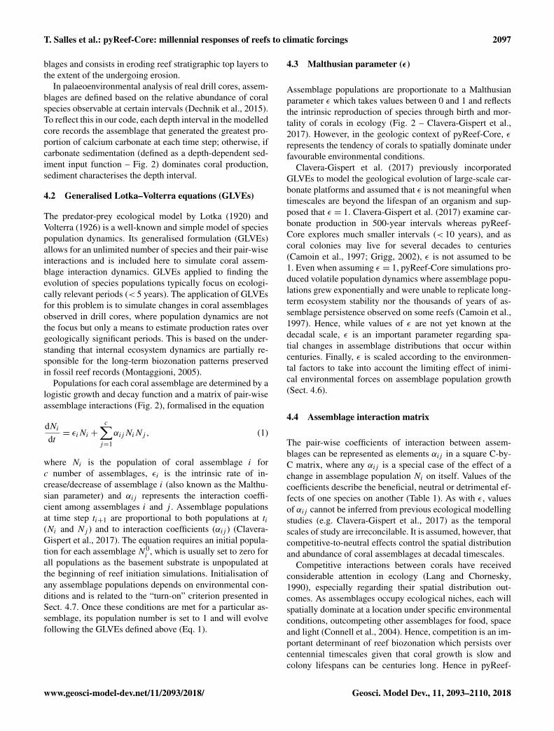
We present a 1-D deterministic, carbonate stratigraphic for-ward model called pyReef-Core that simulates vertical reefsequences comparable to those found in actual fossil reefdrill cores. pyReef-Core is a tool to represent how dy-namic biological and physical processes interact to createpredictable, stratigraphic patterns. As shown in Fig. 2, themain steps in our workflow are as follows: (i) using real geo-logical, geophysical and ecological data to establish environ-mental boundary conditions, vertical accretion rates of coralassemblages and defining assemblage tolerance thresholds toenvironmental factors and (ii) defining model input parame-ters including Malthusian and assemblage interaction matrixparameters, simulation time and those that define model res-olution; before (iii) running the model to create a verticalcore sequence that records assemblage changes and growthhistory.

4.1 Vertical reef accretion module

Carbonate production in a 1-D context, as represented bypyReef-Core, refers to the thickness of calcium carbonateproduced in a core due to vertical framework accretion thatis a result of vertical coral growth and sediment supply(Spencer, 2011). Hence, in this context carbonate productioncorresponds to reef vertical accretion. The model does notconsider the destructional processes that occur on the reefdue to physical, chemical and biological erosion but does ac-count for erosional process during phases of subaerial expo-sure (referred as karstification in the model).

In our model, carbonate production is calculated for eachtime step at a user-defined resolution based on (i) the maxi-mum vertical accretion rate for each assemblage; (ii) GLVEsdetermining assemblage populations; and (iii) the environ-mental conditions that define optimal growth for each assem-blage. During periods of subaerial exposure, karstificationoccurs at a uniform rate independent of the type of assem-



blages and consists in eroding reef stratigraphic top layers tothe extent of the undergoing erosion.

In palaeoenvironmental analysis of real drill cores, assem-blages are defined based on the relative abundance of coralspecies observable at certain intervals (Dechnik et al., 2015).To reflect this in our code, each depth interval in the modelledcore records the assemblage that generated the greatest pro-portion of calcium carbonate at each time step; otherwise, ifcarbonate sedimentation (defined as a depth-dependent sed-iment input function – Fig. 2) dominates coral production,sediment characterises the depth interval.

4.2 Generalised Lotka–Volterra equations (GLVEs)

The predator-prey ecological model by Lotka (1920) andVolterra (1926) is a well-known and simple model of speciespopulation dynamics. Its generalised formulation (GLVEs)allows for an unlimited number of species and their pair-wiseinteractions and is included here to simulate coral assem-blage interaction dynamics. GLVEs applied to finding theevolution of species populations typically focus on ecologi-cally relevant periods (< 5 years). The application of GLVEsfor this problem is to simulate changes in coral assemblagesobserved in drill cores, where population dynamics are notthe focus but only a means to estimate production rates overgeologically significant periods. This is based on the under-standing that internal ecosystem dynamics are partially re-sponsible for the long-term biozonation patterns preservedin fossil reef records (Montaggioni, 2005).

Populations for each coral assemblage are determined by alogistic growth and decay function and a matrix of pair-wiseassemblage interactions (Fig. 2), formalised in the equation

dNidt= εiNi +

c∑j=1

αijNiNj , (1)

where Ni is the population of coral assemblage i forc number of assemblages, εi is the intrinsic rate of in-crease/decrease of assemblage i (also known as the Malthu-sian parameter) and αij represents the interaction coeffi-cient among assemblages i and j . Assemblage populationsat time step ti+1 are proportional to both populations at ti(Ni and Nj ) and to interaction coefficients (αij ) (Clavera-Gispert et al., 2017). The equation requires an initial popula-tion for each assemblage N0

i , which is usually set to zero forall populations as the basement substrate is unpopulated atthe beginning of reef initiation simulations. Initialisation ofany assemblage populations depends on environmental con-ditions and is related to the “turn-on” criterion presented inSect. 4.7. Once these conditions are met for a particular as-semblage, its population number is set to 1 and will evolvefollowing the GLVEs defined above (Eq. 1).

4.3 Malthusian parameter (ε)

Assemblage populations are proportionate to a Malthusianparameter ε which takes values between 0 and 1 and reflectsthe intrinsic reproduction of species through birth and mor-tality of corals in ecology (Fig. 2 – Clavera-Gispert et al.,2017). However, in the geologic context of pyReef-Core, εrepresents the tendency of corals to spatially dominate underfavourable environmental conditions.

Clavera-Gispert et al. (2017) previously incorporatedGLVEs to model the geological evolution of large-scale car-bonate platforms and assumed that ε is not meaningful whentimescales are beyond the lifespan of an organism and sup-posed that ε = 1. Clavera-Gispert et al. (2017) examine car-bonate production in 500-year intervals whereas pyReef-Core explores much smaller intervals (< 10 years), and ascoral colonies may live for several decades to centuries(Camoin et al., 1997; Grigg, 2002), ε is not assumed to be1. Even when assuming ε = 1, pyReef-Core simulations pro-duced volatile population dynamics where assemblage popu-lations grew exponentially and were unable to replicate long-term ecosystem stability nor the thousands of years of as-semblage persistence observed on some reefs (Camoin et al.,1997). Hence, while values of ε are not yet known at thedecadal scale, ε is an important parameter regarding spa-tial changes in assemblage distributions that occur withincenturies. Finally, ε is scaled according to the environmen-tal factors to take into account the limiting effect of inimi-cal environmental forces on assemblage population growth(Sect. 4.6).

4.4 Assemblage interaction matrix

The pair-wise coefficients of interaction between assem-blages can be represented as elements αij in a square C-by-C matrix, where any αij is a special case of the effect of achange in assemblage population Ni on itself. Values of thecoefficients describe the beneficial, neutral or detrimental ef-fects of one species on another (Table 1). As with ε, valuesof αij cannot be inferred from previous ecological modellingstudies (e.g. Clavera-Gispert et al., 2017) as the temporalscales of study are irreconcilable. It is assumed, however, thatcompetitive-to-neutral effects control the spatial distributionand abundance of coral assemblages at decadal timescales.

Competitive interactions between corals have receivedconsiderable attention in ecology (Lang and Chornesky,1990), especially regarding their spatial distribution out-comes. As assemblages occupy ecological niches, each willspatially dominate at a location under specific environmentalconditions, outcompeting other assemblages for food, spaceand light (Connell et al., 2004). Hence, competition is an im-portant determinant of reef biozonation which persists overcentennial timescales given that coral growth is slow andcolony lifespans can be centuries long. Hence in pyReef-



Factor (dimensionless)

Community interac4on matrix

fdepth fsed fflow

min{fdepth, fsed, ftemp, fpH, fnu, fflow} = fenv

0 < fenv < 100 %

Environmental tolerance threshold func4ons for each assemblage Popula4on growth limited by

environmental factors

Repeat for each 4me steps

( 0.1<∆t<0.25 years) from start 4me to present.

t0

tfinal

Sim

ula4

on 4

me

Time layers

Modelled core

fenv1

fenv2

if population = 0: if fenv > fopt: begin growth

Ass

embl

age

1A

ssem

blag

e 2

GLV equa6on

Community popula6on

Carbonate produc6on

Malthusian parameter

Water velocitySediment inputSea level/tectonics

100 %

0 %

100 %

0 %

Tim

e [k

a]

Dep

th [m

bsl]

Dep

th [m

bsl]

25

0

20

15

10

5

25

0

20

15

10

5

0-6-12-10

-8

-6

-4

-2

0

Depth [mbsl]/subs.[m] Accumula4on [m a ]1.e-3 2.e-3 3.e-3

Speed [m s ]0.05 0.15 0.25

Carbonate kars6fica6on

Temperature/pH/nutrients

Tim

e [k

a]

10.50-10

-8

-6

-4

-2

0

-1 -1

(a) (b)

Figure 2. Illustration outlining pyReef-Core workflow (a) and of the resulting simulated core (b). First boundary conditions for sea level,sediment input and flow velocity are set, which describes their relationship to either depth or time. The boundary conditions are usedto establish the environment factor fenv, which describes the proportion of the maximum growth rate that an assemblage can achieve,depending on whether the environmental conditions exceed the optimal conditions for growth. The environment factor is scaled by theMalthusian parameter, which is in turn used as input in the GLVEs to determine assemblage populations. Larger assemblage populationscontribute to a faster rate of vertical accretion (here referred to as carbonate production). At the end of the time step, boundary conditions areupdated and the process is repeated.

Table 1. Interaction possibilities among coral assemblages and the associated range of matrix coefficients, adapted from Clavera-Gispertet al. (2017).

Interactions Effect on i αij range Effect on j αij range

Competition Detrimental −1≤ αij ≤ 0 Detrimental −1≤ αij ≤ 0Neutralism Neutral αij = 0 Neutral αij = 0

Core, the interaction matrix is formed by competitive-to-neutral interaction coefficients between −1 and 0 (Table 1).

4.5 Computing carbonate production based onassemblage populations

Solved GLVEs determine population growth/decline for eachassemblage, and are used to compute carbonate production(cm yr−1) for each time step. The amount of carbonate pro-duced by each coral assemblage during each time step is de-fined as

dpidt=

∑ci=1Ai ×Ni

S, (2)

where the carbonate production at every time step of eachassemblage pi for c number of assemblages is a product ofthe population distribution Ni and the maximum rate of ver-tical accretion Ai in proportion to a scalar S. The scalar isintroduced to the vertical growth equation in order to min-imise distortionary effects of exponential growth trends foreach population occurring in the absence of inter-assemblagecompetition (i.e. to prevent unreasonably large populationgrowth when only one assemblage can exist under certainconditions). Total vertical reef growth G recorded in a coreis the sum of carbonate sediment deposited psed and all cal-



cium carbonate produced by each assemblage:

dGdt=

c∑i=1

pi +psed. (3)

4.6 Environmental factors

Sediment input, water flow and accommodation are the basicenvironmental factors influencing coral growth in pyReef-Core. However, the model architecture is such that in thefuture it is possible to simulate the effect of other impor-tant environmental parameters such as ocean temperature,pH and nutrient flux. Tolerance functions are defined for eachenvironmental factor as a set of four points that indicatesboth the range in which an assemblage would reasonably ex-ist based on published empirical data (Done, 1982; Hopleyet al., 2007; Dechnik, 2016) and the rate at which vertical ac-cretion reduces as the environmental conditions exceed up-per or lower threshold limits for each assemblage (Fig. 2).As such, they define an “optimal growth window” for eachassemblage. The threshold functions for each assemblage toambient environmental conditions are combined into a singleenvironmental parameter fenv subject to the minimum valuerule:

fenv =min[f idepth,f

ised,f

itemp,f

ipH,f

inu,f

iflow

], (4)

where fdepth, fsed, ... and fflow represent the threshold func-tions for each assemblage i. Hence, fenv is seen as the com-bined effect of ambient environmental conditions on optimalgrowth conditions (Fig. 2). Finally, the Malthusian parameterε is scaled by the environmental factor such that

Ei = ε× f ienv, (5)

which reflects the limiting effect on environmental factors onthe growth potential of each assemblage.

4.7 Turn-on criterion

At the initialisation of the pyReef-Core simulations, assem-blage populations are usually set to zero. Population growthonly occurs when the initial criterion fenv > fopt is met(Fig. 2). It reflects the notion that reef turn-on events oc-cur because of a confluence of optimal conditions includ-ing a shallow substrate, favourable energy, light and watertemperature, pH, and nutrients conditions and relatively lowsediment supply (Buddemeier and Hopley, 1988; Fabricius,2005; Dechnik et al., 2015). In other words, pyReef-Coreonly initiates growth when a degree of optimality in growthconditions are met. By default, the value of fopt is set to 0.5which means that the turn-on criterion is met when environ-mental conditions enable at least 50 % of the maximum verti-cal accretion. The parameter, however, can be adjusted withinthe XML input file to reflect different assemblage populationsensitivities to environmental conditions.

5 Examples of model application

Two case studies are presented here to assess the abilityof pyReef-Core to reproduce realistic sequences found indrill core. We simulate the interactions between three assem-blages which are estimated based on water depth intervals(shallow, intermediate and deep). We also consider that coralproduction in these experiments is primarily controlled byaccommodation and exposure to sedimentation (Chappell,1980; Tudhope, 1989) and water flow (Fulton et al., 2005;Comeau et al., 2014).

5.1 Experimental settings for model simulations

5.1.1 Assemblage maximum vertical accretion rates

Maximum vertical accretion rates in the simulation are user-defined. For shallow assemblages on exposed margins, max-imum vertical accretion rates (11 m/kyr) are chosen to re-flect known average rates for robust branching coral faciesin high-energy environments established for the Indo-Pacific(Montaggioni, 2005). Moderate–deep assemblages representslightly higher maximum accretion rates (15 m/kyr) with thelowest accretion rates (9 m/kyr) for deep assemblages. Thesewere chosen to reflect the average accretion rates for Indo-Pacific tabular-branching and massive coral facies found inhigh-energy conditions (Montaggioni, 2005).

5.1.2 Ecological dynamics

pyReef-Core requires knowledge of the intrinsic rate ofassemblage population growth/decline (εi) and the matrixcoefficients (αij ) of interactions between distinct assem-blages. However, inferring ecological dynamics from ecolog-ical studies is challenging. Empirical studies of coral compe-tition and growth are often focused at the species rather thanassemblage level and explain competitive relationships qual-itatively rather than quantitatively (e.g. Connell et al., 2004).Moreover, GLVEs have not been used to model coral popula-tion dynamics at the temporal resolution (centennial to mil-lennial) we are interested in. Based on an initial sensitivityanalysis, we define a set of values for the Malthusian parame-ter (εi) and interaction coefficients among assemblages (αij )which are summarised in Table 2. Chosen coefficients definesmall competitive interactions between assemblages.

The coral assemblages defined in this study largely do notshare the same environmental setting and optimal growthconditions. Therefore, competitive interactions are restrictedto only those assemblages that may reasonably co-exist dueto overlapping depth, sediment flux or flow velocity thresh-olds. This translates to an interaction matrix with values onlyalong the main diagonal and the super- and sub-diagonals.Everywhere else, interactions are set to 0. Associated withthese interactions, we define a series of critical threshold re-sponse functions for each assemblages (Fig. 3).



Figure 3. Environmental threshold functions for shallow,moderate–deep and deep assemblages characteristic of a syn-thetic exposed margin. The x axis indicates the limitation onmaximum vertical accretion for conditions outside the optimalmaximum vertical accretion rate.

5.1.3 Depth threshold functions

Based on a statistical analysis of the depth and environmentaldistribution of modern coral communities at One Tree Reef(GBR), Dechnik et al. (2017) calibrated the palaeo-water de-positional environments of six fossil coral assemblages (threein protected and three in exposed environments). This cali-bration was also based on quantitative measurements of crus-tose coralline algae thickness and vermetid gastropod abun-dance which are reliable palaeo-depth indicators, allowingfor the depth intervals to be more accurately constrained.These assemblages are broadly consistent with shallow- anddeep-water coral facies of the Indo-Pacific (Cabioch et al.,1999; Camoin et al., 2012).

Here, three assemblages typically occurring on exposedslopes are modelled according to the estimated depth in-tervals defined by Dechnik (2016) (Table 2) and rep-resent shallow-water (< 6 m), moderate-to-deep-water (6–20 m) and deep-water (20–30 m) assemblages.

5.1.4 Water flow

The water flow function is constructed according to the the-oretical relationship defined by Chappell (1980) wherebywave stress decreases exponentially with depth (Fig. 4).Here, we rely on the velocity–depth relationships on wave-exposed reef slopes from the field study by Sebens et al.

Dept

h [m

]

Tim

e [k

y]

Water depth [m] Sediment input [m d ]Flow velocity [m s ]

1.e-3 2.e-3 3.e-31.e-1 2.e-1-10 -5 0

0

5

10

15

20

25

-8

-7

-6

-5

-4

-3

-2

-1 -1(a) (b)

Figure 4. The curve in (a) shows the Holocene sea-level curve es-timated from Sloss et al. (2007). The graphs in (b) illustrate theboundary conditions established for flow velocity and sediment in-put used in the experimental simulations.

(2003). A maximum velocity of 25 cm s−1 in region ≤ 1 mand an exponential decrease up to 25 m below which flowvelocity is set to 0. This is consistent with direct observa-tions from exposed algal flat (Davies and Hopley, 1983) andmaximum velocities (> 50 cm s−1) beyond which branchingcorals are susceptible to breakage (Baldock et al., 2014).

With specific data on the optimal flow environment forspecific corals lacking, assumptions about thresholds for dis-tinct coral assemblages are inferred from boundary condi-tions. That is, the water flow exposure threshold range foreach assemblage reflects the attenuation of water flow withdepth (Fig. 3).

5.1.5 Sediment exposure

pyReef-Core can model the vertical sedimentation rate(m day−1) as a function of either time or depth. When sedi-ment flux is dependent on depth, it implies that sediments areautochthonous (loose carbonate materials), in contrast to ter-rigenous sediments transported from outside the reef system(siliclastic materials), which may be represented by sedimentflux varying with time. In our case studies, we use a depth-dependent sedimentation rate input curve to approximate thetemporal variations in sediment accumulation along the core(Fig. 4).

Sediment tolerance thresholds for each coral assemblage(Fig. 3) are informed by Dechnik et al. (2017) before receiv-ing maximum and minimum sedimentation rates correspond-ing to the sediment input boundary condition (Fig. 4). Theboundary condition provides a broad indicator of the sedi-ment load expected at certain depths and thus what would betolerated for each depth-specific assemblage. With alternatesediment input boundary conditions, the upper and lowertolerance thresholds can be adjusted to represent how coralcommunities respond differently to site-specific suspendedsediment levels.



Table 2. Parameter values used in our two experiments. Estimates of maximum production rates for assemblages were determined based onliterature surveys of maximum growth rates for coral facies of GBR (Davies and Hopley, 1983) and Indo-Pacific reefs (Montaggioni, 2005).

Parameter Values

Malthusian parameter εi = 0.004

Assemblage interaction matrix

Main diagonal Detrimental - αii =−0.0005Sub- and super-diagonal Detrimental - αij =−0.0001

Assemblage maximum growth rate (m yr1)

Shallow-water assemblage (0–6 m) 0.011Moderate–deep-water assemblage (6–20 m) 0.012Deep-water assemblage (20–30 m) 0.009

Assemblage threshold tolerance variables

Shallow-water assemblage (0–6 m)Absolute water flow threshold range 0.05≤ fflow ≤ 0.3Absolute sediment input threshold range 0≤ fsed ≤ 0.003

Moderate–deep-water assemblage (6–20 m)Absolute water flow threshold range 0≤ fflow ≤ 0.12Absolute sediment input threshold range 0.0015≤ fsed ≤ 0.003

Deep-water assemblage (20–30 m)Absolute water flow threshold range 0≤ fflow ≤ 0.08Absolute sediment input threshold range 0.0023≤ fsed ≤ 0.0045

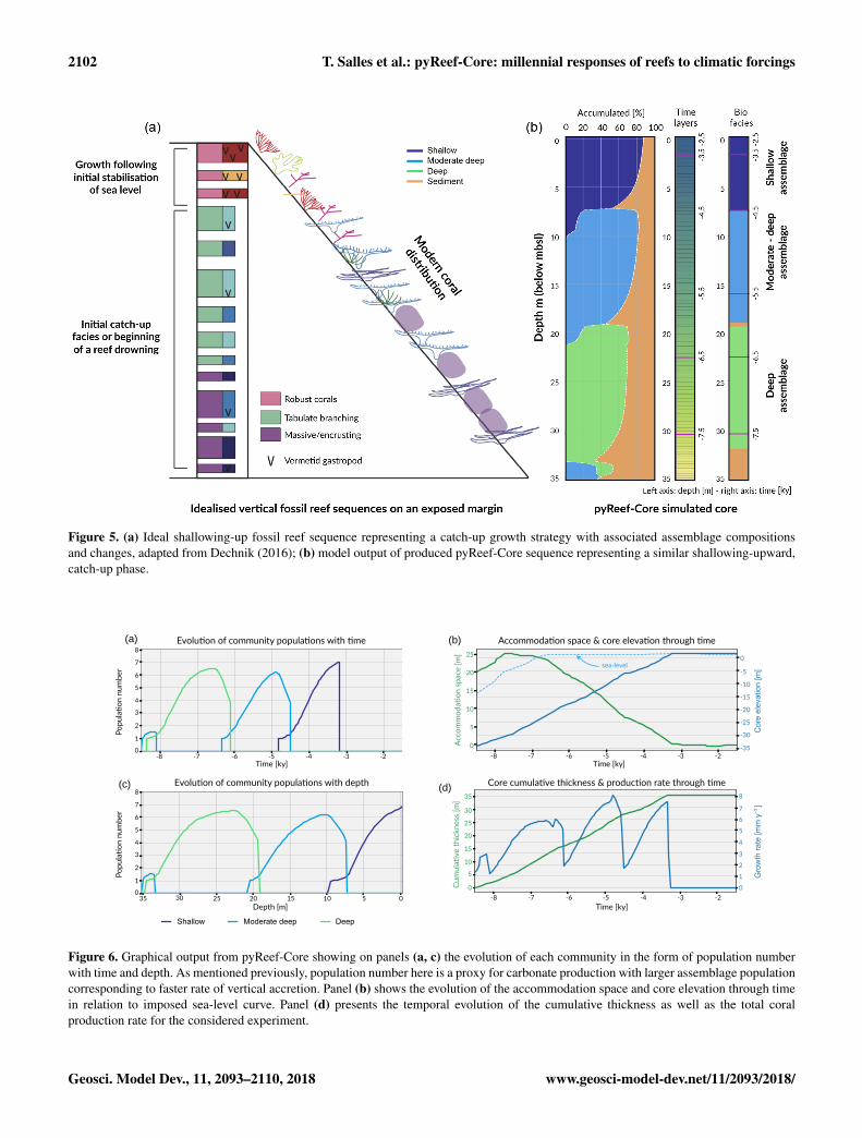
5.2 Case 1: GBR idealised windwardshallowing-upward Holocene reef sequence

Based on the afore-described experimental settings, we firstsimulate a typical shallowing-up sequence of coral assem-blages on the exposed rims of several reef in the GBR, ex-pressing a catch-up strategy of reef growth during Holocenesea-level rise (∼ 9.4 ka to present).

5.2.1 Initial parameters

Considering the simulated temporal scale, neither subsidencenor uplift are considered to be important (Hopley et al.,2007) in this experiment. Instead, accommodation is simu-lated as a function of Holocene sea-level changes and verti-cal coral reef growth only. The Holocene relative sea-level(RSL) curve from Sloss et al. (2007) is used to represent sea-level change (Fig. 4). The data suggest a RSL history that ischaracterised by a mid-Holocene highstand of 1.8 m at∼ 4 kabefore returning slowly to present sea level, matching otherestimates of RSL (Chappell, 1983; Lewis et al., 2013).

Simulation begins at 8.5 ka, which is within the take-offenvelope for Holocene growth of outer-platform GBR reefs(Hopley et al., 2007). At 8.5 ka, RSL is 15 m below sea level(Sloss et al., 2007) and substrate is at 20 m depth in order tosimulate a catch-up growth strategy from a deep substrate.We compute the GLVEs at time intervals of 2.5 years andcombine each accumulated assemblage as a stratigraphic unitwithin the core for every 50 years.

5.2.2 Communities evolution and synthetic corerepresentation

Figure 5 presents the GBR-representative assemblages sum-marised by Dechnik (2016) as well as the simulated core bypyReef-Core. The modelled core is 35 m long and is com-posed of three assemblages characteristic of an exposed mar-gin and carbonate sediments. The simulation portrays twodistinct assemblage transitions from massive assemblagesrepresenting deep (20–30 m), low-flow conditions to a faster-growing, tabular-and-branching assemblage characteristic ofthe 6–20 m depth interval, which is succeeded in shallow wa-ter (< 6 m) by a robust-branching assemblage representinghigher-energy conditions (Figs. 6, 5).

As sea level rises from 8.5 to 6.5 ka, the deeper assem-blages have sufficient accommodation space (> 20 m) andlow-flow to thrive. However, greater sediment input at depthis inhibitive in the early part of the simulation at the base ofthe core (32–35 m) (Fig. 5). As sea level begins to stabilise(Fig. 6b), accommodation space decreases and moderate–deep assemblages start to dominate the sequence up to 4.7 ka(Fig. 6c). Following stabilisation from 4.7 to 3.2 ka, shal-low assemblages develop as a result of the decreased ac-commodation space (∼ 6 m at 4.7 ka), high-velocity hydro-dynamic conditions and reduced sediment input. Assemblagegrowth rates (Fig. 6d) show a pattern similar to the popula-tion number curves with values lower than assemblage max-imum production rates (Table 2) indicative of the effects of



Figure 5. (a) Ideal shallowing-up fossil reef sequence representing a catch-up growth strategy with associated assemblage compositionsand changes, adapted from Dechnik (2016); (b) model output of produced pyReef-Core sequence representing a similar shallowing-upward,catch-up phase.

Evolu&on of community popula&ons with &me

Evolu&on of community popula&ons with depth

Accommoda&on space & core eleva&on through &me

Core cumula&ve thickness & produc&on rate through &me

Popu

la&o

n nu

mbe

rPo

pula

&on

num

ber

Time [ky]

Depth [m] Time [ky]

Time [ky]

Acco

mm

oda&

on s

pace

[m]

Cum

ula&

ve th

ickn

ess

[m]

Cor

e el

evat

ion

[m]

Gro

wth

rate

[mm

y

]

sea-level

0

1

2

3

4

5

6

7

8

0

1

2

3

4

5

6

7

8

-8 -7 -6 -5 -4 -3 -2

-8 -7 -6 -5 -4 -3 -2-8 -7 -6 -5 -4 -3 -2

35 30 25 20 15 10 5 00

5

10

15

20

25

30

35

0

1

2

3

4

5

67

8

0

5

10

15

20

25 0

-5

-10

-15

-20

-25

-30

-35

DeepModerate deepShallow

-1

(a) (b)

(c) (d)

Figure 6. Graphical output from pyReef-Core showing on panels (a, c) the evolution of each community in the form of population numberwith time and depth. As mentioned previously, population number here is a proxy for carbonate production with larger assemblage populationcorresponding to faster rate of vertical accretion. Panel (b) shows the evolution of the accommodation space and core elevation through timein relation to imposed sea-level curve. Panel (d) presents the temporal evolution of the cumulative thickness as well as the total coralproduction rate for the considered experiment.



Evolu&on of community popula&ons with &me

Evolu&on of community popula&ons with depth

Accomoda&on space & core eleva&on through &me

Core cumula&ve thickness & produc&on rate through &me

Popu

la&o

n nu

mbe

r

Shallow Moderate deep Deep

Popu

la&o

n nu

mbe

r

Time [ky]

Depth [m] Time [ky]

Time [ky]

Acco

mod

a&on

spa

ce [m

]Cu

mul

a&ve

thic

knes

s [m

]

sea-level

0

1

2

3

4

5

6

7

8

0

1

2

3

4

5

6

7

8

-140 -120 -100 -80 -60 -40 -20

80 70 60 50 40 30 10 0

0

20

40

60

80

0

2

4

6

8

-60

-40

-20

20

40

60 0

-20

-40

-60

-80

-100

0 -140 -120 -100 -80 -60 -40 -20 0

-140 -120 -100 -80 -60 -40 -20 020

0

(a) (b)

(c) (d)

Cor

e el

evat

ion

[m]

Gro

wth

rate

[mm

y

]-1

Figure 7. Similar to the previous case, these graphs shows in panels (a, c) the evolution of each community in the form of population numberwith time and depth. Panel (b) shows the evolution of the accommodation space and core elevation through time in relation to the imposedsea-level curve. Panel (d) presents the temporal evolution of the cumulative thickness as well as the total coral production rate.

environmental factors (sediment input and flow velocity) onthe growth of each assemblage. The deeper assemblage is15 m thick and is composed of 30–60 % loose sediment andis succeeded by ∼ 12 m of moderate–deep assemblages witha lesser proportion of sediment (Fig. 5). The last 6–7 m ofcore are predominantly formed by shallow assemblages withon average less than 20 % of carbonate sediments (Fig. 5).The simulated shallowing-up sequence accurately reflectsexpected shift from deep to moderately deep assemblages at∼ 15–20 m depth and from moderately deep to shallow as-semblages at ∼ 6 m depth proposed by Cabioch et al. (1999)and Dechnik (2016). The simulated sequence relates wellto the description proposed by Dechnik (2016) and repro-duces the distinct assemblages defined in the idealised reefsequences found on exposed margin along the GBR (Fig. 5).

The modelled core reaches sea level at around 2.5 ka(Fig. 6) which also correlates well with values reported forseveral reefs in the GBR (Davies and Hopley, 1983; Dechniket al., 2015; Salas-Saavedra et al., 2018). Average verticalaccretion rate implied by the model is around 4.1 m kyr−1

(Fig. 6), again in the range of actual drill cores average rates,which varies by around 3 to 5 m kyr−1 on exposed reef mar-gins (Davies and Hopley, 1983; Camoin et al., 2012; Dech-nik et al., 2015). It is also worth noting that coral growthbecomes predominant within the sequence at ∼ 7.8 ka in themodelled core, which coheres with the observed delay in reefinitiation of approximately 1 kyr (Dechnik et al., 2015) afterinitial flooding of the substrate during the Holocene trans-gression. We also notice that the transitions between assem-blages also correspond to periods where the proportion ofcarbonate sediment deposited increases (Fig. 5). It mimicsa lag between optimal conditions from one assemblage tothe other and relates to the choice of environmental thresh-old functions that were imposed in our simulation (Fig. 3).

Overall, the model reproduces the details of the formation ofshallowing-upward sequences both in terms of assemblagessuccession, accretion rates, deposited thicknesses and tim-ing of initiation. It can be applied to estimate the impact ofchanging environmental conditions on growth rates and pat-terns under many different settings and initial conditions.

5.3 Case 2: GBR idealised reef core reconstructionover the last 140 kyr

For the second study case, the experimental settings forthreshold functions, ecological dynamics, water flow andsediment exposure (presented in Sect. 5.1) remain un-changed. The goal is not to match a specific drill core butto illustrate the influence of forcing conditions on the devel-opment of a coral reef sequence with our model.

5.3.1 Initial parameters

We reconstruct using pyReef-Core the evolution of an idealcoral reef sequence since the last interglacial (LIG). LIG isrepresented by marine isotope stage (MIS) 5e, which is aproxy record of low global ice volume and high sea level(Grant et al., 2012). It is arbitrarily set to begin at approx-imately 130 ka before present and our simulation runs over140 kyr. The GLVEs which control the coral productions dy-namic are updated every 25 years and stratigraphic layers arerecorded at time interval of 100 years.

Here we use the sea-level curve proposed by Grant et al.(2012), who estimate sea-level records based on the timingof past ice-volume changes, relative to polar climate change.The relative sea-level change over the simulated period hasrates of rise reaching 12 cm yr−1 during all major phases ofice-volume reduction, with values below 7 mm yr−1 when



sea level exceeded present mean sea level (Grant et al., 2012).The applied sea-level curve is shown in Fig. 7b.

The karstification of Pleistocene reef limestone has beenidentified as a controlling factor on variations in antecedenttopography, which in turn is thought to influence the mor-phology of modern reefs (Purdy and Winterer, 2001). Ratesof karstification are a function of exposure time, rainfall,porosity and original topography of exposed carbonate reefs.Summary of karstification rates from both the Indo-Pacificand Caribbean shows values ranging from 0.01 m kyr−1 (Bar-bados, Hopley et al., 2007) to 0.14 m kyr−1 (mid–outer plat-form reefs, southern GBR; Marshall and Davies, 1982). Herewe impose a karstification rate of 0.07 m kyr−1 consistentwith estimates from Ribbon Reef 5 and outer central GBRshelf (Webster, 1999).

Over such a period of time, sea-level fluctuations are notthe only factor controlling the accommodation change anduplift–subsidence evolution has to be considered (Spencer,2011). Based on a comprehensive study of GBR reefs, Dech-nik (personal communication, 2017) estimates that a subsi-dence rate of ∼ 0.083 to 0.13 m kyr−1 is required to explainthe observed elevation of the upper surface of the LIG reefthat provides the antecedent topography of the modern mid–outer platform reefs in the GBR. The proposed range is con-sistent with values found for other reefs along the GBR (Mar-shall and Davies, 1982; Webster, 1999). In our model, we usea constant rate of subsidence set to 0.1 m kyr−1 that corre-sponds to 14 m of subsidence over the duration of the sim-ulation. In addition, the initial elevation is set 20 m abovesea-level position at the start of the simulation (140 ka), cor-responding to a depth of ∼ 70 m below the current sea-levelposition.

5.3.2 Communities evolution and synthetic corerepresentation

Prior to 135 ka, the model shows a first stage of reef growthcharacterised by shallow-water, high-energy coral commu-nity colonisation (Fig. 7a,c and Fig. 8), following the flood-ing of the antecedent platform. The cumulative thickness forthis phase is < 10 m (Fig. 7d) and is compatible with val-ues estimated for Ribbon Reef 5 and Heron Island (Dechniket al., 2017).

Following this initial phase, a deepening-upward sequenceoccurs up to 132 ka (Fig. 8). Again, this sequence has alsobeen identified in a similar time interval at One Tree Reef(southern GBR) and Stanley Reef (central GBR) (Dechniket al., 2017). A lack of significant reef framework (< 30 %)characterises the stratigraphic sequence during this interval.

The rapid sea-level rise (Grant et al., 2012) during the endof the penultimate deglaciation explains the drowning eventobserved in the core from 128 to 118 ka (Fig. 7c). Duringthis period, the accommodation increase is mainly driven bysea-level fluctuations and to a small extent (∼ 1 m) by theimposed subsidence rate.

From 118 to 107 ka, during the first stage of the regressionphase, a shallowing-upward sequence (∼ 30 m thick) is iden-tified with three distinct community populations modelledover time (Fig. 7c). During this time interval, the maximumpopulation number for the moderate–deep assemblages isrelative lower (< 3) than for the two other assemblages (> 7).Consequently, the percentage of accumulated thickness forthis assemblage is below 7 %. These assemblage transitionsare primarily controlled by high-frequency sea-level varia-tions observed in the Grant et al. (2012) curve (Fig. 7b). Mi-nor events of karstification (< 2 cm of erosion) are triggeredby short episodes of subaerial exposure around 110 ka. From107.5 to 104 ka, high-energy coral communities (shallow as-semblages) dominate the sequence with a maximum growthrate above 8 mm yr−1 (Fig. 7d).

The following stage from 107 to 12 ka is characterised bya period of subaerial exposure due to sea-level fall (Fig. 7d).Both subsidence and karstification occur and account fornearly 11 m of elevation offset with about 1 m attributedto karstification processes (Fig. 8). Applied to a real case,pyReef-Core can be used to test several scenarios with differ-ent rates of subsidence and karstification in order to explainfor example the discrepancy in age–elevation data of LIGdeposits observed in the GBR (Marshall and Davies, 1982;Dechnik et al., 2017). It can also be used to estimate the con-tribution of karst dissolution and subsidence (Hopley et al.,2007; Purdy and Winterer, 2001) with a more quantitive ap-proach.

By 13 ka, sea level re-floods the LIG reef, and Holocenereef growth initiates ∼ 10.5 ka in the experiment (Fig. 7).The lag (2.5 kyr) between flooding and reef growth initia-tion matches well with observations for the GBR (Fabricius,2005; Hopley et al., 2007; Camoin et al., 2012). However, thetiming of the initial flooding occurs 3 kyr earlier than whatis expected for the GBR. This temporal difference is relatedto both sea-level variations (Grant et al., 2012) and choseninitial starting elevation of the model. The Holocene reef se-quence is around 46 m thick (Fig. 8), which is above most ofthe GBR reef maximum vertical accretion thicknesses (usu-ally < 30 m) but correlates with thicknesses found in reefsfrom Tahiti and Huon Peninsula (Woodroffe and Webster,2014). This Holocene sequence is first composed of morethan 30 m of moderate–deep assemblage, which correspondsto the catch-up phase discussed in the first study case andis associated with the rapid sea-level rise. The reef accretionrate during this time interval is maximal and reaches valuesabove 8.2 mm y−1 (Fig. 7d). The remaining ∼ 15 m of theuppermost sequence is built of shallow assemblages that be-come predominant after 6 ka when sea-level rise decreases. Itis also worth noting the presence of short periods of subaerialexposure which coincide with two small karstification events(karst dissolution < 1 cm; Fig. 8).

The total simulated core has an overall thickness > 86 m.A complete sequence such as the one modelled here is un-likely to be found in a natural reef complex mainly due to



Thickness [m] Propor1on [%] Strat. abundance [%]

Time layers

Bio. faciesKarst. [m]

Dep

th b

elow

pre

sent

mea

n se

a-le

vel [

m]

Two last cores axes le-: depth [m] right: 7me[ky]

Shallow Moderate deep Deep Sediment

0.0 0.2 0.4 0.6 0.8 0 20 40 60 80 100 0 20 40 60 80 100 0 0.5 1

0

10

20

30

40

50

60

70

80

0

10

20

30

40

50

60

70

80

0

10

20

30

40

50

60

70

80

0

10

20

30

40

50

60

70

80

0

10

20

30

40

50

60

70

80

-138

-132

-114

-112

-110

-108

-106

-10

-8

-6

-4

-2

Figure 8. Simulated reef core reconstruction, showing the different stages of last interglacial reef growth in relation to sea level, karstificationand subsidence.

the 3-D nature of such a system (Woodroffe and Webster,2014). Nevertheless the predicted sequence represents in 1-D the idealised succession of coral assemblages producedfor a given set of initial and forcing conditions. Therefore, itcan be compared to series of drill cores at different positionsalong a given region and used as a quantitative approach toanalyse stratigraphic responses of coral reefs to a combina-tion of physical, biological and sedimentological processes.

6 Discussion

Relatively little is known about how coral reefs grow andrespond to environmental conditions at temporal scales ex-ceeding what is measurable (i.e. observational record overthe last 100 years) (Hughes et al., 2017). It has been a majorchallenge for both geological and ecological studies to ade-quately capture coral reef ecological and environmental dy-namics on centennial to millennial temporal scales and at reefscales (Stocker et al., 2013). Our new method, pyReef-Core,



operates on these scales and offers a coherent, fast and effec-tive way to predict 1-D reef core stratigraphies and assem-blages changes. It can be used to improve our understandingof coral reef response to climatic and environmental changes(Done, 2011; Harris et al., 2015). The code is most usefulin application to reef researchers examining the vertical dis-tribution of coral assemblages and coral growth dynamics(Montaggioni, 2005; Camoin et al., 2012; Dechnik, 2016) bycomparing outputs between modelling cores. This would en-able the extrapolation of knowledge gained from examiningdrill cores to areas of the reef where data are scarce. It canalso be used to understand environmental histories of coreswhere dating or classification of assemblages is difficult dueto poor core recovery. Despite its 1-D limitation, the modelcan be applied to gain a 3-D picture of the environmental,ecological and geomorphological history of a specific reef.This can be achieved by defining multiple biological and en-vironmental initial conditions representing, for example, thedifferences in assemblage types and hydrodynamic condi-tions between the windward and leeward margins of the reef(Cabioch et al., 1999; Dechnik et al., 2015; Salas-Saavedraet al., 2018).

Necessarily, pyReef-Core is also a simplified representa-tion of a coral reef system and required a number of freeparameters such as sediments, flow, Malthusian parameter,and community matrix parameter which need to be definedfor modelling. The task of finding this set of parameters thatbest describes a specific reef site and core data is challengingfor several reasons. Firstly, empirical estimates of environ-mental tolerance thresholds of given assemblages are scarcein the scientific literature making their estimation difficult(Camoin et al., 2012; Baldock et al., 2014; Dechnik et al.,2017). Therefore, results interpreted from the modelled envi-ronmental threshold represent hypotheses that must be testedand validated against additional real, physical measurementson reefs. Secondly, reefs experience a variety of natural sedi-mentation regimes due to the variable morphologies (Hopleyet al., 2007) and flow regimes due to the position of reefsin respect to the dominant swell (Dechnik, 2016) and prox-imity to the coast (Larcombe et al., 2001). Consequently, itis difficult to construct a model that fully represents com-plex reef system dynamics simultaneously. Thirdly, the esti-mation of the interaction matrix coefficients and Malthusianparameters remains difficult (Clavera-Gispert et al., 2017),specifically when considering coral assemblage dynamics atthe temporal scale (decadal to centennial) relevant to pyReef-Core. Yet interpretations of these parameters from ecolog-ical modelling studies provide a useful guide with regardto reef biozonation and assemblage competition (Lang andChornesky, 1990; Grigg, 2002; Connell et al., 2004). Finally,modelled vertical accretion or growth patterns in pyReef-Core are non-linear reflecting the natural complexity of coralreef systems and the biological and physical interactions oc-curring at reef scales. It poses the problems for calibrationsand the underlying uncertainties inherent in our simplified

approach (Burgess and Wright, 2003; Warrlich et al., 2008;Clavera-Gispert et al., 2017). Nevertheless, our model rep-resents a shift from the standard accommodation-forced ge-ometrical models (Dalmasso et al., 2001; Gale et al., 2002;Burgess et al., 2006) where coral reef stratigraphy is con-trolled mainly by changes in sea level. Even if our approachis a simplification of natural processes, the simulated strati-graphic patterns are a sum of simultaneous, interacting tec-tonic, biological, physical and sedimentological processes.

pyReef-Core can be described as a multidimensional (i.e.many parameters) and multi-modal (i.e. non-unique solu-tions) forward model where numerous combinations of in-teracting parameters could potentially produce identical se-quences (Burgess et al., 2006; Burgess and Prince, 2015).Given a specific reef core dataset and pyReef-Core, the taskof finding the model parameter space that best describes thereef core data can be defined as the inverse modelling prob-lem (Jessell, 2002). Mosegaard and Sambridge (2002) high-lighted the importance for Monte Carlo methods in analysisof non-linear inverse problems where no analytical expres-sion for the forward relation between data and model param-eters is available. Markov chain Monte Carlo (MCMC) meth-ods can straightforwardly quantify uncertainty in model as-sumptions and parameters (Andrieu et al., 2003). This is par-ticularly useful for SFM approaches (Warrlich et al., 2008)that require optimisation techniques that lack uncertaintyquantification. However, Bayesian inference methods haverarely been applied to reef modelling, despite evidence oftheir usefulness when handling models with complex, inter-relating parameters (Gallagher et al., 2009). A useful applica-tion of such approach would involve the optimisation of en-vironmental threshold and ecological modelling parametersand then parameterising the sediment input and fluid flowboundary conditions based on empirical measurements.

7 Conclusions

Bridging the gap between ecologists’ and geologists’ viewsof coral reef system dynamics is challenging. In this pa-per, we present pyReef-Core, a 1-D deterministic, carbon-ate SFM that simulates vertical reef sequences comparableto those found in actual drill cores. The model serves as abasis for investigating the relationship between the key bio-logical processes (i.e. the function of coral assemblages in-teractions based on the GLVEs) involved in coral reef growthand the influence of changing environmental factors (e.g. sealevel, tectonics, ocean temperature, pH and nutrient). Thesignificance of the approach lies in its ability to incorporatecoral community dynamics into reef growth modelling andunderstand the responses of coral reefs to environmental dis-turbances on centennial to millennial timescales at the reefscale. The exploration of these intermediate scales is crucialto better understand the enduring growth response of coralsin the face of climatic and environmental changes that are



expected to have lasting impacts on reefs into the future. Asshown in the case studies, generated model predictions co-here well with data and provide a means for explaining ob-served assemblage patterns. It can help to better constrain thetolerance of shallow-water corals to long-term environmen-tal disturbance and to quantify the relative dominance of sealevel, tectonics, as well as hydrodynamic energy and sedi-ment input on reef growth.

Code and data availability. The source code (writtenin Python 2.7.6) with examples (Jupyter Notebooks)is archived as a repository on Github and Zenodo(https://doi.org/10.5281/zenodo.1080115). The code is licensedunder the GNU General Public License v3.0. The easiest wayto use pyReef-Core is via our Docker container (searching forpyreef-docker on Kitematic), which is shipped with the completelist of dependencies and the case studies presented in this paper.

Competing interests. The authors declare that they have no conflictof interest.

Acknowledgements. We would like to thank the anonymousreviewer and Jon Hill for their insightful comments on the paper.Tristan Salles was supported by ARC IH130200012, Jody M.Webster was supported by ARC DP120101793, and Tristan Sallesand Jody M. Webster were also supported by SREI2020 grants.This research was undertaken with the assistance of resourcesfrom the National Computational Infrastructure (NCI), which issupported by the Australian Government and from Artemis HPCGrand Challenge supported by the University of Sydney.

Edited by: Guy MunhovenReviewed by: Jon Hill and one anonymous referee

References

Abbey, E., Webster, J. M., and Beaman, R. J.: Geomorphology ofsubmerged reefs on the shelf edge of the Great Barrier Reef: Theinfluence of oscillating Pleistocene sea-levels, Mar. Geol., 288,61—78, 2011.

Andrieu, C., De Freitas, N., Doucet, A., and Jordan, M. I.: An intro-duction to MCMC for machine learning, Mach. Learn., 50, 5–43,2003.

Baldock, T. E., Golshani, A., Callaghan, D. P., Saunders, M. I., andMumby, P. J.: Impact of sea-level rise and coral mortality on thewave dynamics and wave forces on barrier reefs, Mar. Pollut.Bull., 83, 155–164, 2014.

Barrett, S. J. and Webster, J. M.: Reef Sedimentary Accretion Model(ReefSAM): Understanding coral reef evolution on Holocenetime scales using 3D stratigraphic forward modelling, Mar.Geol., 391, 108–126, 2017.

Bosence, D. and Waltham, D.: Computer modeling the internal ar-chitecture of carbonate platforms, Geology, 18, 26–30, 1990.

Bosscher, H. and Southam, J.: CARBPLAT – A computer model tosimulate the development of carbonate platforms, Geology, 20,235–238, 1992.

Braithwaite, C. J. R.: Coral-reef records of Quaternary changes inclimate and sea-level, Earth-Sci. Rev., 156, 137–154, 2016.

Bruno, J. F. and Edmunds, P. J.: Metabolic consequences of pheno-typic plasticity in the coral Madracis mirabilis (Duchassaing andMichelotti): the effect of morphology and water flow on aggre-gate respiration, J. Exp. Mar. Biol. Ecol., 229, 187–195, 1998.

Buddemeier, R. and Hopley, D.: Turn-ons and turn-offs: Causesand mechanisms of the initiation and termination of coral reefgrowth, Proc. 6th International Coral Reef Symposium, 8–12 Au-gust 1988, Townsville, Australia, Plenary Addressess and Statusreview, 1988.

Burgess, P. M. and Prince, G. D.: Non-unique stratal geometries:implications for sequence stratigraphic interpretations, BasinRes., 27, 351–365, 2015.

Burgess, P. M. and Wright, V. P.: Numerical Forward Modelingof Carbonate Platform Dynamics: An Evaluation of Complex-ity and Completeness in Carbonate Strata, J. Sediment. Res., 73,637–652, 2003.

Burgess, P. M., Lammers, H., van Oosterhout, C., and Granjeon, D.:Multivariate sequence stratigraphy: Tackling complexity and un-certainty with stratigraphic forward modeling, multiple scenar-ios, and conditional frequency maps, AAPG Bulletin, 90, 1883–1901, 2006.

Cabioch, G., Camoin, G. F., and Montaggioni, L. F.: Postglacialgrowth history of a French Polynesian barrier reef tract, Tahiti,central Pacific, Sedimentology, 46, 985–1000, 1999.

Camoin, G. F., Colonna, M., Montaggioni, L. F., Casanova, J.,Faure, G., and Thomassin, B. A.: Holocene sea level changesand reef development in the southwestern Indian Ocean, CoralReefs, 16, 247–259, 1997.

Camoin, G. F., Seard, C., Deschamps, P., Webster, J. M., Abbey,E., Braga, J. C., Iryu, Y., Durand, N., Bard, E., Hamelin,B., Yokoyama, Y., Thomas, A. L., Henderson, G. M., andDussouillez, P.: Reef response to sea-level and environmentalchanges during the last deglaciation: Integrated Ocean DrillingProgram Expedition 310, Tahiti Sea Level, Geology, 40, 643–646, 2012.

Chappell, J.: Coral morphology, diversity and reef growth, Nature,286, 249–252, 1980.

Chappell, J.: A revised sea-level record for the last 300,000 yearsfrom Papua New Guinea, Search, 14, 99–101, 1983.

Clavera-Gispert, R., Gratacós, Ò., Carmona, A., and Tolosana-Delgado, R.: Process-based forward numerical ecological model-ing for carbonate sedimentary basins, Comput. Geosci., 21, 373–391, 2017.

Comeau, S., Edmunds, P. J., Lantz, C. A., and Carpenter,R. C.: Water flow modulates the response of coral reef com-munities to ocean acidification, Scientific Reports, 4, 6681,https://doi.org/10.1038/srep06681, 2014.

Connell, J. H., Hughes, T. P., Wallace, C. C., Tanner, J. E., Harms,K. E., and Kerr, A. M.: A long-term study of competition anddiversity of corals, Ecol. Monogr., 74, 179–210, 2004.

Cubasch, U., Wuebbles, D., Chen, D., Facchini, M. C., Frame, D.,Mahowald, N., and Winther, J.-G.: Climate Change 2013: ThePhysical Science Basis. Contribution of Working Group I to theFifth Assessment Report of the Intergovernmental Panel on Cli-


https://github.com/pyReef-model/pyReefCore

https://doi.org/10.5281/zenodo.1080115

https://hub.docker.com/r/pyreefmodel/pyreef-docker/

https://doi.org/10.1038/srep06681


mate Change, Cambridge University Press, Cambridge, UnitedKingdom and New York, NY, USA, 2013.

Dalmasso, H., Montaggioni, L. F., Bosence, D., and Floquet, M.:Numerical Modelling of Carbonate Platforms and Reefs: Ap-proaches and Opportunities, Energ. Explor. Exploit., 19, 315–345, 2001.

Davies, P. J. and Hopley, D.: Growth fabrics and growth-rates ofHolocene reefs in the Great Barrier-Reef, BMR J. Aust. Geol.Geop., 8, 237–251, 1983.

Davies, P. J., Marshall, J. F., and Hopley, D.: Relationship betweenreef growth and sea level in the Great Barrier Reef, ProceedingsOf The Fifth International Coral Reef Congress. Tahiti, 27 May–1 June 1985, 3, 95–103, 1985.

Dechnik, B.: Evolution of the Great Barrier Reef over the last130 ka: a multifaceted approach, integrating palaeo ecological,palaeo environmental and chronological data from cores, PhDthesis, School of Geosciences, The University of Sydney, Aus-tralia, 2016.

Dechnik, B., Webster, J., Davies, P., Braga, J., and Reimer, P.:Holocene turn-on and evolution of the Southern Great BarrierReef: Revisiting reef cores from the Capricorn Bunker Group,Mar. Geol., 363, 174–190, 2015.

Dechnik, B., Webster, J., Webb, G. E., Nothdurft, L., Dutton, A.,Braga, J.-C., Zhao, J.-X., Duce, S., and Sadler, J.: The evolu-tion of the Great Barrier Reef during the Last Interglacial Period,Global Planet. Change, 149, 53–71, 2017.

Done, T.: Patterns in the distribution of coral communities acrossthe central Great Barrier Reef, Coral Reefs, 1, 95–107, 1982.

Done, T.: Encyclopedia of Modern Coral Reefs: Structure, Formand Process, chap. Corals: environmental controls on growth,edited by: Hopley, D., Springer, Netherlands, Dordrecht, 2011.

Dullo, W.-C.: Coral growth and reef growth: a brief review, Facies,51, 33–48, 2005.

Erftemeijer, P. L. A., Riegl, B., Hoeksema, B. W., and Todd, P. A.:Environmental impacts of dredging and other sediment distur-bances on corals: A review, Mar. Pollut. Bull., 64, 1737–1765,2012.

Fabricius, K. E.: Effects of terrestrial runoff on the ecology of coralsand coral reefs: review and synthesis, Mar. Pollut. Bull., 50, 125–146, 2005.

Falter, J. L., Atkinson, M. J., and Merrifield, M. A.: Mass-transferlimitation of nutrient uptake by a wave-dominated reef flat com-munity, Limnol. Oceanogr., 49, 1820–1831, 2004.

Flügel, E.: New Perspectives in Microfacies, Springer Berlin Hei-delberg, Berlin, Heidelberg, 1–6, 2004.

Fulton, C. J., Bellwood, D. R., and Wainwright, P. C.: Wave energyand swimming performance shape coral reef fish assemblages,P. Roy. Soc. Lond. B Bio., 272, 827–832, 2005.

Gale, A. S., Hardenbol, J., Hathway, B., Kennedy, W. J., Young,J. R., and Phansalkar, V.: Global correlation of Cenomanian (Up-per Cretaceous) sequences: Evidence for Milankovitch controlon sea level, Geology, 30, 291–294, 2002.

Gallagher, K., Charvin, K., Nielsen, S., Sambridge, M., andStephenson, J.: Markov Chain Monte Carlo (MCMC) samplingmethods to determine optimal models, model resolution andmodel choice for earth science problems, Mar. Petrol. Geol., 26,525–535, 2009.

Gischler, E.: Quaternary reef response to sea-level and environmen-tal change in the western Atlantic, Sedimentology, 62, 429–465,2015.

Granjeon, D. and Joseph, P.: Numerical Experiments in Stratigra-phy: Recent Advances in Stratigraphic and Sedimentologic Com-puter Simulations, chap. Concepts and applications of a 3-D mul-tiple lithology, diffusive model in stratigraphic modeling, editedby: Harbaugh, J. W., Watney, W. L., Rankey, E. C., Slingerland,R., Goldstein, R. H., and Franseen, E. K., SEPM Special Publi-cation, 4, 2, https://doi.org/10.1126/sciadv.aao4350, 1999.

Grant, K. M., Rohling, E. J., Bar-Matthews, M., Ayalon, A.,Medina-Elizalde, M., Ramsey, C. B., Satow, C., and Roberts,A. P.: Rapid coupling between ice volume and polar temperatureover the past 150,000 years, Nature, 491, 744–747, 2012.

Grigg, R. W.: Precious corals in Hawaii: discovery of a new bed andrevised management measures for existing beds, Ecol. Monogr.,64, 13–20, 2002.

Grossman, E. E. and Fletcher, C. H.: Holocene reef developmentwhere wave energy reduces accommodation, J. Sediment. Res.,74, 49–63, 2004.

Hallock, P.: Coral Reefs, Carbonate Sediments, Nutrients, andGlobal Change, in: The History and Sedimentology of AncientReef Systems, edited by: Stanley, G. D., Springer US, Boston,MA, 387–427, 2001.

Harris, D. L., Vila-Concejo, A., Webster, J. M., and Power, H. E.:Spatial variations in wave transformation and sediment entrain-ment on a coral reef sand apron, Mar. Geol., 363, 220–229, 2015.

Harris, D. L., Rovere, A., Casella, E., Power, H. E., Canavesio,R., Collin, A., Pomeroy, A., Webster, J. M., and Parravicini, V.:Coral reef structural complexity provides important coastal pro-tection from waves under rising sea levels, Science Advance, 4,eaao4350 https://doi.org/10.1126/sciadv.aao4350, 2018.

Hill, J., Tetzlaff, D., Curtis, A., and Wood, R.: Modeling shallowmarine carbonate depositional systems, Comput. Geosci., 35,1862–1874, 2009.

Hill, J., Wood, R., Curtis, A., and Tetzlaff, D. M.: Preservation offorcing signals in shallow water carbonate sediments, Sediment.Geol., 275–276, 79–92, 2012.

Hopley, D., Smithers, S. G., and Parnell, K. E.: The Geomorphologyof the Great Barrier Reef: development, diversity and change,Cambridge, United Kingdom, 2007.

Houlbrèque, F. and Ferrier-Pagès, C.: Heterotrophy in TropicalScleractinian Corals, Biol. Rev., 84, 1–17, 2009.

Huang, X., Griffiths, C. M., and Liu, J.: Recent development instratigraphic forward modelling and its application in petroleumexploration, Australian J. Earth Sci., 62, 903–919, 2015.

Hubbard, D. K.: Sedimentation as a control of reef development: St.Croix, U.S.V.I., Coral Reefs, 5, 117–125, 1986.

Hughes, T. P.: Geology and ecology of coral reefs, Trends Ecol.Evol., 15, p. 125, 2000.

Hughes, T. P., Kerry, J. T., Álvarez-Noriega, M., Álvarez-Romero,J. G., Anderson, K. D., Baird, A. H., Babcock, R. C., Beger, M.,Bellwood, D. R., Berkelmans, R., Bridge, T. C., Butler, I. R.,Byrne, M., Cantin, N. E., Comeau, S., Connolly, S. R., Cumming,G. S., Dalton, S. J., Diaz-Pulido, G., Eakin, C. M., Figueira,W. F., Gilmour, J. P., Harrison, H. B., Heron, S. F., Hoey, A. S.,Hobbs, J.-P. A., Hoogenboom, M. O., Kennedy, E. V., Kuo, C.-y.,Lough, J. M., Lowe, R. J., Liu, G., McCulloch, M. T., Malcolm,H. A., McWilliam, M. J., Pandolfi, J. M., Pears, R. J., Pratchett,


https://doi.org/10.1126/sciadv.aao4350

https://doi.org/10.1126/sciadv.aao4350


M. S., Schoepf, V., Simpson, T., Skirving, W. J., Sommer, B.,Torda, G., Wachenfeld, D. R., Willis, B. L., and Wilson, S. K.:Global warming and recurrent mass bleaching of corals, Nature,543, 373–377, 2017.

Jessell, M.: Three-dimensional geological modelling of potential-field data, Comput. Geosci., 27, 455–465, 2002.

Kayanne, H., Yamano, H., and Randall, R. H.: Holocene sea-levelchanges and barrier reef formation on an oceanic island, PalauIslands, western Pacific, Sediment. Geol., 150, 47–60, 2002.

Kench, P.: Encyclopedia of Modern Coral Reefs: Structure, Formand Process, chap. Sediment Dynamics, edited by: Hopley, D.,Springer Netherlands, Dordrecht, 994–1005, 2011.

Kendall, C. G. S. C., Strobel, J., Cannon, R., Bezdek, J., and Biswas,G.: The simulation of the sedimentary fill of basins, J. Geophys.Res., 96, 6911–6929, 1991.

Kleypas, J. A., McManus, J. W., and Meñez, L. A. B.: Environmen-tal Limits to Coral Reef Development: Where Do We Draw theLine?, American Zoologist, 39, 146–159, 1999.

Kuffner, I. B.: Effects of ultraviolet radiation and water motion onthe reef coral Porites compressa Dana: a flume experiment, Mar.Biol., 138, 467–476, 2001.

Lang, J. C. and Chornesky, E. A.: Competition between sclerac-tinian reef corals – A review of mechanisms and effects, Else-vier Science Publishing Company, Inc., Amsterdam, The Nether-lands, 209–252, 1990.

Larcombe, P., Costen, A., and Woolfe, K. J.: The hydrodynamicand sedimentary setting of nearshore coral reefs, central GreatBarrier Reef shelf, Australia: Paluma Shoals, a case study, Sedi-mentology, 48, 811–835, 2001.

Lewis, S. E.and Sloss, C. R., Murray-Wallace, C. V., Woodroffe,C. D., and Smithers, S. G.: Post-glacial sea-level changes aroundthe Australian margin: a review, Quaternary Sci. Rev., 74, 115–138, https://doi.org/10.1016/j.quascirev.2012.09.006, 2013.

Lotka, A. J.: Elements of Physical Biology, Williams and Wilkins,Baltimore, 1920.

Lowe, R. J. and Falter, J. L.: Oceanic Forcing of Coral Reefs, Annu.Rev. Mar. Sci., 7, 43–66, 2015.

Madin, J. S. and Connolly, S. R.: Ecological consequences of ma-jor hydrodynamic disturbances on coral reefs, Nature, 444, 477–480, 2006.

Marshall, J. F. and Davies, P. J.: Internal structure and holocene evo-lution of one tree reef, southern great barrier reef, Coral Reefs,1, 21–28, 1982.

Montaggioni, L. F.: History of Indo-Pacific coral reef systems sincethe last glaciation: Development patterns and controlling factors,Earth-Sci. Rev., 71, 1–75, 2005.

Mosegaard, K. and Sambridge, M.: Monte carlo analysis of inverseproblems, Inverse Probl., 18, R29, https://doi.org/10.1088/0266-5611/18/3/201, 2002.

Neumann, A. C. and Macintyre, I. G.: Reef response to sea levelrise: Keep-up, catch-up or give-up, Proceedings Of The Fifth In-ternational Coral Reef Congress, Tahiti, 27 May–1 June 1985, 3,105–110, 1985.

Nordlund, U.: FUZZIM: forward stratigraphic modeling made sim-ple, Comput. Geosci., 25, 449–456, 1999.

Paola, C.: Quantitative models of sedimentary basin filling, Sedi-mentology, 47, 121–178, 2000.

Parcell, W. C.: Evaluating the Development of Upper Jurassic Reefsin the Smackover Formation, Eastern Gulf Coast, U.S.A. through

Fuzzy Logic Computer Modeling, J. Sediment. Res., 73, 498–515, 2003.

Paulay, G. and McEdward, L. R.: A simulation model of island reefmorphology: the effects of sea level fluctuations, growth, subsi-dence and erosion, Coral Reefs, 9, 51–62, 1990.

Perry, C. T. and Larcombe, P.: TMarginal and non-reef-buildingcoral environments, Coral Reefs, 22, 427–432, 2003.

Perry, C. T., Smithers, S. G., Palmer, S. E., Larcombe, P., and John-son, K. G.: 1200 year paleoecological record of coral communitydevelopment from the terrigenous inner shelf of the Great BarrierReef, Geology, 36, 691–694, 2008.

Precht, W. F. and Aronson, R. B.: Stability of Reef-Coral Assem-blages in the Quaternary, edited by: Hubbard, D. K., Rogers, C.S., Lipps, J. H., and Stanley Jr., G. D., Springer Netherlands, Dor-drecht, 155–173, 2016.

Purdy, E. G. and Winterer, E. L.: Origin of atoll lagoons, GSA Bul-letin, 113, 837–854, 2001.

Rogers, C. S.: Sublethal and lethal effects of sediments applied tocommon Caribbean Reef corals in the field, Mar. Pollut. Bull.,14, 378–382, 1983.

Rogers, C. S.: Responses of coral reefs and reef organisms to sedi-mentation, Mar. Ecol. Prog. Ser., 185–202, 1990.

Rogers, J. S., Monismith, S. G., Koweek, D. A., and Dunbar, R. B.:Wave dynamics of a Pacific Atoll with high frictional effects,J. Geophys. Res.-Oceans, 121, 350–367, 2016.

Salas-Saavedra, M., Dechnik, B., Webb, G. E., Webster, J. M., Zhao,J.-X., Nothdurft, L. D., Clark, T. R., Graham, T., and Duce, S.:Holocene reef growth over irregular Pleistocene karst confirmsmajor influence of hydrodynamic factors on Holocene reef de-velopment, Quaternary Sci. Rev., 180, 157–176, 2018.

Salles, T., Griffiths, C., Dyt, C., and Li, F.: Australian shelf sedi-ment transport responses to climate change-driven ocean pertur-bations, Mar. Geol., 282, 268–274, 2011.

Salles, T., Ding, X., and Brocard, G.: pyBadlands: A frameworkto simulate sediment transport, landscape dynamics and basinstratigraphic evolution through space and time, PLOS ONE, 13,1–24, 2018a.

Salles, T., Ding, X., Webster, J. M., Vila-Concejo, A., Brocard,G., and Pall, J.: A unified framework for modelling sedi-ment fate from source to sink and its interactions with reefsystems over geological times, Scientific Reports, 8, 5252,https://doi.org/10.1038/s41598-018-23519-8, 2018b.

Sanders, D. and Baron-Szabo, R. C.: Scleractinian assemblages un-der sediment input: their characteristics and relation to the nutri-ent input concept, Palaeogeogr. Palaeocl., 216, 139–181, 2005.

Schlager, W.: Carbonate Sedimentology and Sequence Stratigra-phy, SEPM Society for Sedimentary Geology, SEPM Conceptsin Sedimentology and Paleontology No. 8, 200 pp., 2005.

Schwarzacher, W.: Sedimentation in Subsiding Basins, Nature, 210,1349–1350, 1966.

Seard, C., Borgomano, J., Granjeon, D., and Camoin, G.: Impact ofenvironmental parameters on coral reef development and drown-ing: Forward modelling of the last deglacial reefs from Tahiti(French Polynesia; IODP Expedition 310), Sedimentology, 60,1357–1388, 2013.

Sebens, K. P., Helmuth, B., Carrington, E., and Agius, B.: Effectsof water flow on growth and energetics of the scleractinian coralAgaricia tenuifolia in Belize, Coral Reefs, 22, 35–47, 2003.


https://doi.org/10.1016/j.quascirev.2012.09.006

https://doi.org/10.1088/0266-5611/18/3/201

https://doi.org/10.1088/0266-5611/18/3/201

https://doi.org/10.1038/s41598-018-23519-8


Sloss, C. R., Murray-Wallace, C. V., and Jones, B. G.: Holocenesea-level change on the southeast coast of Australia: a review,The Holocene, 17, 999–1014, 2007.

Spencer, T.: Encyclopedia of Modern Coral Reefs: Structure, Formand Process, chap. Glacial Control Hypothesis, edited by: Hop-ley, D., Springer Netherlands, Netherlands, Dordrecht, 2011.

Stafford-Smith, M. G.: Sediment-rejection efficiency of 22 speciesof Australian scleractinian corals, Marine Biology, 115, 229–243, 1993.

Stocker, T., Qin, D., Plattner, G.-K., Tignor, M., Allen, S.,Boschung, J., Nauels, A., Xia, Y., Bex, V., and Midgley, P.: Cli-mate Change 2013: The Physical Science Basis. Contribution ofWorking Group I to the Fifth Assessment Report of the Inter-governmental Panel on Climate Change, Cambridge UniversityPress, Cambridge, United Kingdom and New York, NY, USA,2013.

Tudhope, A. W.: Shallowing-upwards sedimentation in a coral reeflagoon, Great Barrier Reef of Australia, J. Sediment. Res., 59,1036–1051, 1989.

Veron, J. E. N.: Encyclopedia of Modern Coral Reefs: Structure,Form and Process, chap. Corals, in: Biology, Skeletal Deposition,and Reef-Building, edited by: Hopley, D., Springer Netherlands,Dordrecht, 2011.

Volterra, V.: Fluctuations in the abundance of a species consideredmathematically, Nature, 118, 558–560, 1926.

Warrlich, G., Bosence, D., Waltham, D., Wood, C., Boylan, A., andBadenas, B.: 3D stratigraphic forward modelling for analysis andprediction of carbonate platform stratigraphies in exploration andproduction, Mar. Petrol. Geol., 25, 35–58, 2008.

Webster, J. M.: The response of coral reefs to sea level change: evi-dence from the Ryukyu islands and the Great Barrier Reef, PhDthesis, School of Geosciences, The University of Sydney, Aus-tralia, 328 pp., 1999.

Weitzman, J. S., Aveni-Deforge, K., Koseff, J. R., and Thomas,F. I. M.: Uptake of dissolved inorganic nitrogen by shallow sea-grass communities exposed to wave-driven unsteady flow, Mar.Ecol. Prog. Ser., 475, 65–83, 2013.

Wolanski, E., Fabricius, K., Spagnol, S., and Brinkman, R.: Finesediment budget on an inner-shelf coral-fringed island, GreatBarrier Reef of Australia, Estuar. Coast. Shelf S., 65, 153–158,2005.

Woodroffe, C. D. and Webster, J. M.: Coral reefs and sea-levelchange, Mar. Geol., 352, 248–267, 2014.


Date post:	31-May-2020
Category:	Documents
Upload:	others
View:	2 times
Download:	0 times

Exploring coral reef responses to millennial-scale ... · ster,2017), and SIMSAFADIM-CLASTIC...

Documents