35
Exploring Microbes in the Sea Alma Parada Postdoctoral Scholar Stanford University
| Date post: | 09-Apr-2018 |
| Category: |
Documents |
| Upload: | phungduong |
| View: | 218 times |
| Download: | 2 times |

Exploring Microbes in the Sea
Alma Parada
Postdoctoral Scholar
Stanford University

Cruising the ocean to get us some microbes

It’s all about the Microbe!
• Microbes = microorganisms• an organism that requires a microsocope to see
• These can be Bacteria, Archaea, Eukaryotes or Viruses
Archaea
Bacteria
Eukaryotes
http://www.doddhollow.com/biology/lab14.php3

How tiny is a microbe?1cm
Munn C (2011) Microbes in the Marine Environment. Mar Microbiol Ecol Appl:1–24.
4
1mm = 1/10 cm
1mm = 1/10,000 cm
= 0.000001 meter
1mm

Where do the microbes live?
Water Column
Sediment
http://io9.gizmodo.com/5874762/the-ocean-floor-is-like-a-rainforest-where-feces-and-dead-animals-rain-from-the-sky

Getting microbes from the water using Niskin bottles!

Getting Water Column Microbes
Subsample different depths

Use Pressure to push water through filters
0.2mm pore size1mm pore size

Microbial Community DirectedResearch Questions
Now that we’ve captured our microbes on filters…..
• What is the microbial community composition?• Who is there, when and why?
• How dynamic is the microbial community?• Does the community change over time or in response to environmental changes?
• What are the interactions that shape the microbial community?• How do microbes affect each other? How does the environment affect microbes?

Methods to Evaluate a Microbial Community• One important
method: DNA!• An organism’s DNA
contains all of the genes (information) it needs to live
• These genes include those that code for ribosomes!• This is where proteins
are built!• 2-unit structure made
of ribosomal RNA (rRNA) and Proteins
• The rRNA occurs in 3 chunks- one of which is the 16S
http://www.biologyexams4u.com/2013/02/difference-between-70s-and-80s-ribosomes.html#.WWvVu3qFkgs

16S rRNA Molecule• Loops are sequences that can
mutate more easily• Makes them variable between related
groups of organisms • i.e. phylogenetic group
• Therefore the sequence of 16S rDNAof the these hypervariable regions allow us to distinguish phylogenetic groups from each other
• Stems are sequence regions less prone to mutation• Makes them conserved between
groups of organisms• These are candidate regions for
Polymerase Chain Reaction (PCR) primers to target many phylogenetic groups
Yarza P, et al. (2014). Nature Reviews Microbiology 12: 635–645.
Loops
Stems

Sequencing the 16S rDNA• PCR Amplification
• Extract DNA from environment• This contains the genomes from all
microorganisms in the sample
• Uses primers to target 16S rDNA regions of each genome and make lots of copies (amplicons)
• Sequencing• Can use different platforms to
determine the sequence of all those 16S rDNA amplicons
• Bioinformatics• Use the amplicon sequences to
determine identify of the microbes
• Use information added to the primers to determine which sequences belong to different samples
Jo J, Kennedy EA, Kong HH. (2016). J Invest Dermatol 136: e23–e27.

Getting from 16S rDNA sequences to microbe identity • Because PCR and sequencing can introduce errors in the 16S rDNA sequences we
need methods to distinguish between errors and real sequence (genetic) diversity
• 16S rDNA sequences are commonly clustered by sequence similarity into • Operational Taxonomic Units (OTUs)
• The term “operational” comes form the idea, that how that taxonomic unit is defined can be flexible
• The term OTU is most commonly used in reference to groups of similar 16S rRNA gene (rDNA) sequences
• Typically an OTU is considered to define a cluster of sequences that originate from a single type of microbe • Of course this is not always true, but new methods are developed all the time to get us to approach the
coveted OTU=Species or Strain

How do we make an OTU?: Sequence Clustering• Making Operational Taxonomic Units
• Common strategies:• Reference Based: compare sequences to reference set, discard all other sequences
• De novo based: use the sequences to determine how the clusters are formed
• These common strategies require user defined similarity thresholds• Essentially, you choose an algorithm that will cluster the sequences into OTUs based on a
sequence similarity cutoff that you have chosen
• Most common similarity is 97% OTUs, but since sequences that are 97% similar can group together organisms that are quite different, it is not uncommon to require a greater similarity threshold to define an OTU (ie. 99% OTUs or Unique Sequences)
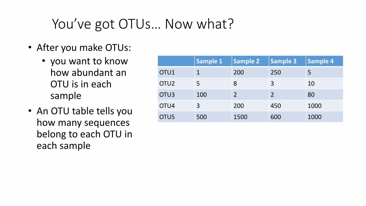
You’ve got OTUs… Now what?
Sample 1 Sample 2 Sample 3 Sample 4
OTU1 1 200 250 5
OTU2 5 8 3 10
OTU3 100 2 2 80
OTU4 3 200 450 1000
OTU5 500 1500 600 1000
• After you make OTUs:
• you want to know how abundant an OTU is in each sample
• An OTU table tells you how many sequences belong to each OTU in each sample

Making an OTU table usableOTU Sequences per Sample
Sample 1 Sample 2 Sample 3 Sample 4
OTU1 1 200 250 5
OTU2 5 8 3 10
OTU3 100 2 2 80
OTU4 3 200 450 1000
OTU5 500 1500 600 1000
• To allow us to compare the OTU abundance between samples:
• One method is to:• Rescale sequence counts to
relative abundance
• Calculate Percent Relative Abundance for each OTU in each sample
OTU % Relative Abundance per sample
= 100(𝑂𝑇𝑈 𝑆𝑒𝑞𝑢𝑒𝑛𝑐𝑒 𝐶𝑜𝑢𝑛𝑡 𝑖𝑛 𝑆𝑎𝑚𝑝𝑙𝑒
𝐴𝑙𝑙 𝑆𝑒𝑞𝑢𝑒𝑛𝑐𝑒𝑠 𝑖𝑛 𝑆𝑎𝑚𝑝𝑙𝑒)
• But what is the identity of each OTU?
OTU % Relative Abundance per Sample
Sample 1 Sample 2 Sample 3 Sample 4
OTU1 0.16 10.47 19.16 0.24
OTU2 0.82 0.42 0.23 0.48
OTU3 16.42 0.10 0.15 3.82
OTU4 0.49 10.47 34.48 47.73
OTU5 82.10 78.53 45.98 47.73
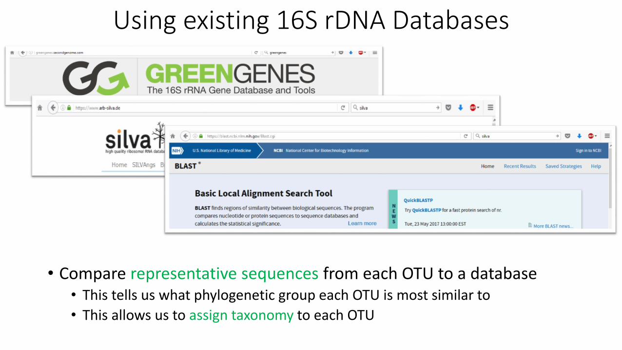
Using existing 16S rDNA Databases
• Compare representative sequences from each OTU to a database• This tells us what phylogenetic group each OTU is most similar to
• This allows us to assign taxonomy to each OTU

OTU Table becomes a window into theMicrobial Community
• Now we can get back to our research questions!
OTU % Relative Abundance per Sample
Sample 1 Sample 2 Sample 3 Sample 4
Nitrosopumilusmaritimus
0.16 10.47 19.16 0.24
Prochlorococcus 0.82 0.42 0.23 0.48
Euryarchaea 16.42 0.10 0.15 3.82
SAR11 0.49 10.47 34.48 47.73
Unknown 82.10 78.53 45.98 47.73
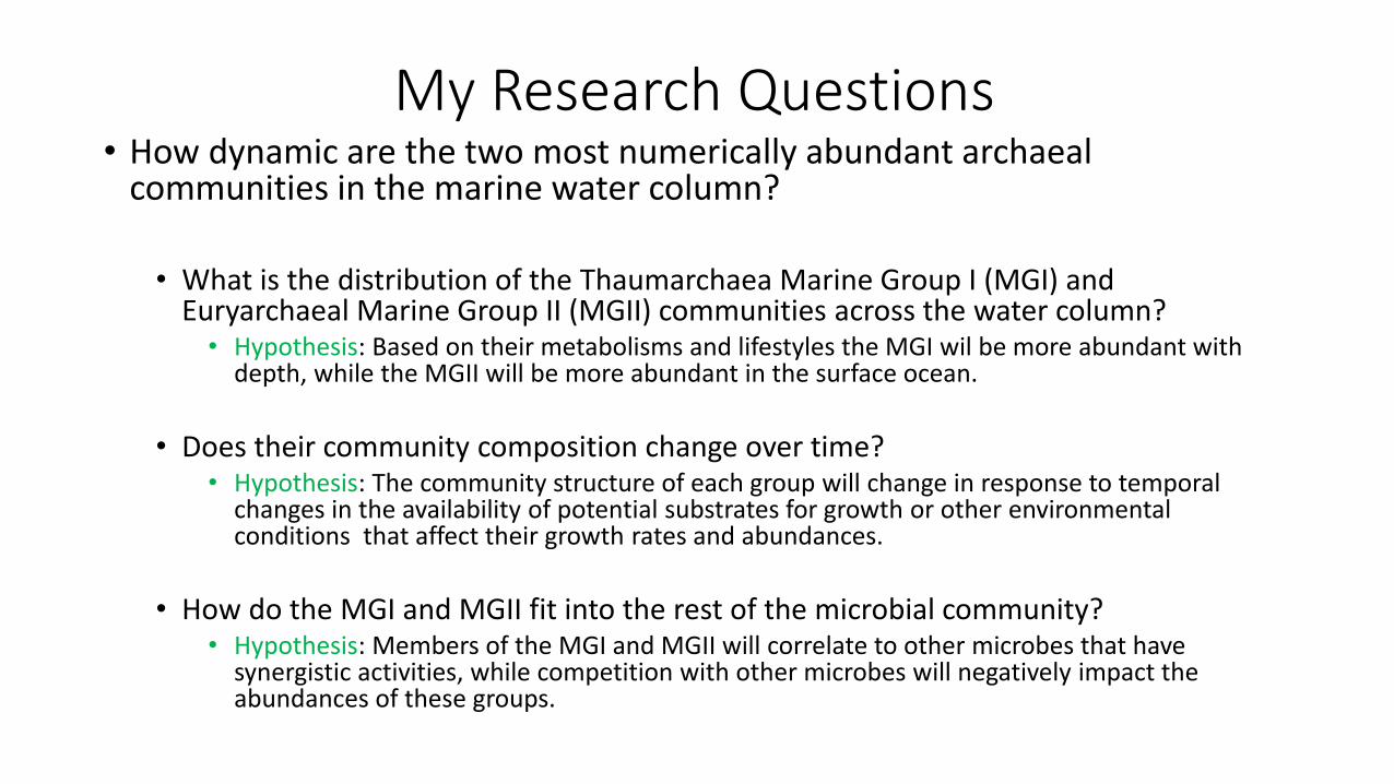
My Research Questions• How dynamic are the two most numerically abundant archaeal
communities in the marine water column?
• What is the distribution of the Thaumarchaea Marine Group I (MGI) and Euryarchaeal Marine Group II (MGII) communities across the water column?• Hypothesis: Based on their metabolisms and lifestyles the MGI wil be more abundant with
depth, while the MGII will be more abundant in the surface ocean.
• Does their community composition change over time?• Hypothesis: The community structure of each group will change in response to temporal
changes in the availability of potential substrates for growth or other environmental conditions that affect their growth rates and abundances.
• How do the MGI and MGII fit into the rest of the microbial community?• Hypothesis: Members of the MGI and MGII will correlate to other microbes that have
synergistic activities, while competition with other microbes will negatively impact the abundances of these groups.

• Let’s take a quick step back
• Who are the MGI and MGII and what do we know about them?
Thaumarchaea MGI and Euryarchaea MGII

Tree of life• A 3-domain system formally proposed by Carl Woese and colleagues 1990 (PNAS)
21
•Concept developed in 1977

• A 3-domain system proposed by Carl Woese and colleagues 1990 through use of the 16S rRNA gene
22
•All Cultured Representatives are Extremophiles
Crenarchaeota:EuryarchaeotaExclusively Thermophiles
Based on cultures
Tree of life

Thaumarchaea MGI found throughout the ocean! So not just an extremophile!
• Not only not an extremophile, evidence showed many MGI are autotrophs that have an important role in the nitrogen cycle
• (e.g. Karner et al. 2001, Pearson et al. 2001, Ouverney et al. 2000, Venter et al 2004)
Lam et al (2007). PNAS
23

Thaumarchaea MGI found throughout the ocean! So not just an extremophile!
• Not only not an extremophile, evidence showed many MGI are autotrophs that have an important role in the nitrogen cycle
• (e.g. Karner et al. 2001, Pearson et al. 2001, Ouverney et al. 2000, Venter et al 2004)
• Nitrosopumilus maritimus: isolate that performs autotrophic ammonia oxidation
• Könneke et al (2005)
Lam et al (2007). PNAS
24
Ammonia Oxidation

MGII life is more unclear
• Their genomes indicate heterotrophic lifestyles• e.g. Iverson et al. 2012, Orsi et al. 2015, Martin-Cuadrado et al. 2015
• Incubation experiments show incorporation of organic carbon• Orsi et al. 2015, 2016
• However, all of our genetic information comes from organisms living in the photic zone
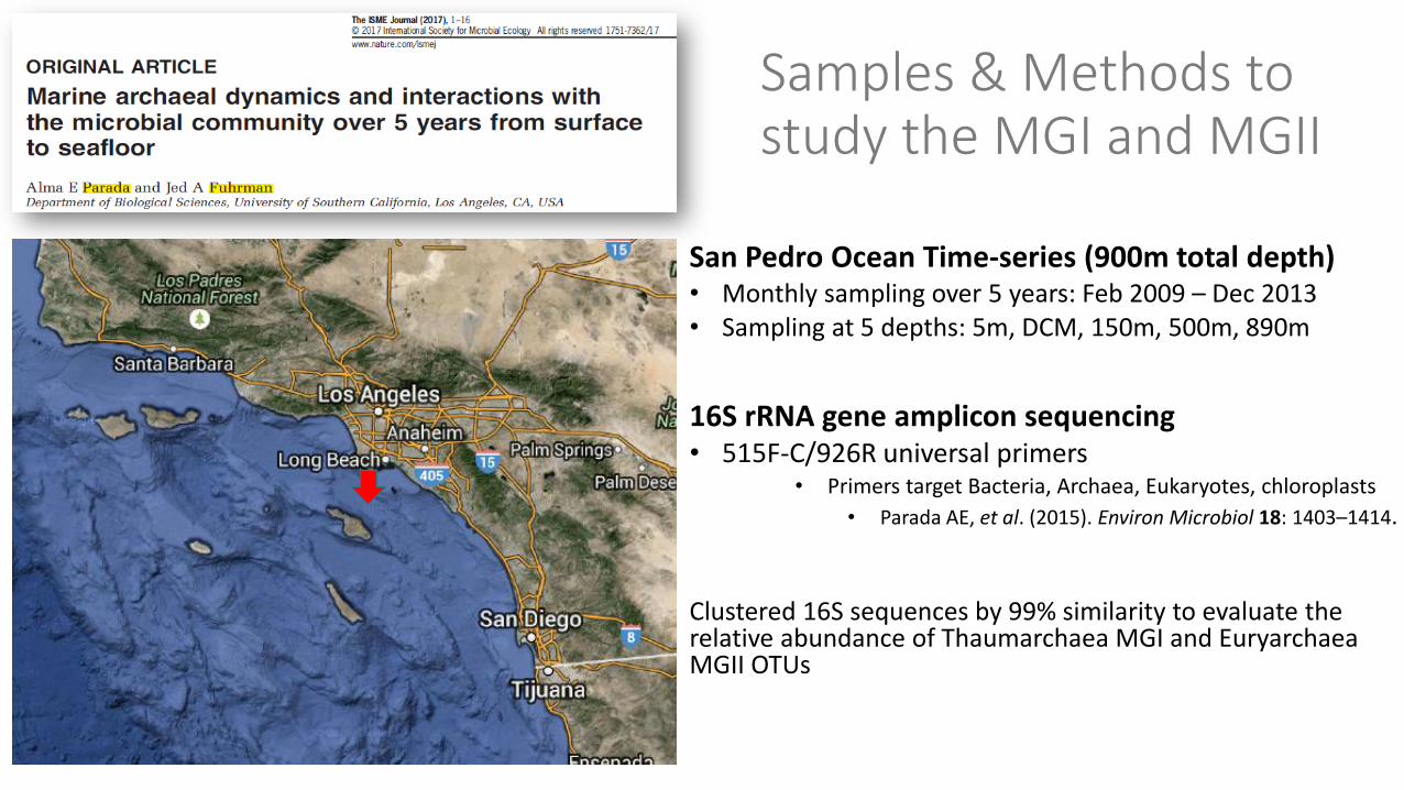
Samples & Methods to study the MGI and MGII
San Pedro Ocean Time-series (900m total depth)• Monthly sampling over 5 years: Feb 2009 – Dec 2013• Sampling at 5 depths: 5m, DCM, 150m, 500m, 890m
16S rRNA gene amplicon sequencing• 515F-C/926R universal primers
• Primers target Bacteria, Archaea, Eukaryotes, chloroplasts
• Parada AE, et al. (2015). Environ Microbiol 18: 1403–1414.
Clustered 16S sequences by 99% similarity to evaluate the relative abundance of Thaumarchaea MGI and EuryarchaeaMGII OTUs

Research Question 1: What is the distribution of the Thaumarchaea Marine Group I and Euryarchaeal Marine Group II communities across the water column?
Ordination plots visually represent the similarities between communities in each sample.
Heatmap shows abundances over time and depth as an alternative to line graphs or barcharts.
Conclusions: • The MGI and MGII display temporal dynamics.• The MGI and MGII communities are stratified across the water
column.

Research Question 2: Does their community composition change over time?
Figure shows the community similarity between every pair of samples at different time lags
Conclusions:
• All depths show increases in similarity at 12month intervals and decreases at 6month intervals
• Statistical tests show communities at all depths demonstrate seasonality.
• The MGI and MGII communities are seasonally variable at all depths at SPOT
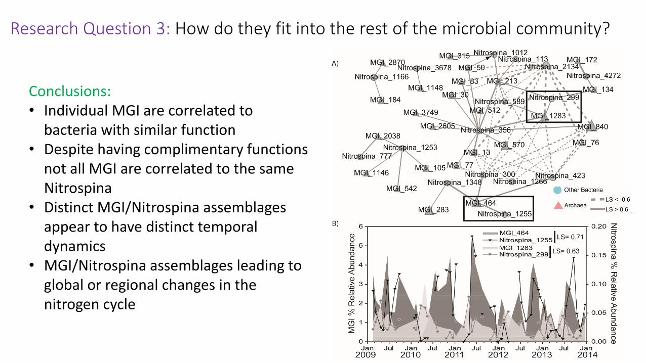
Research Question 3: How do they fit into the rest of the microbial community?
Conclusions:• Individual MGI are correlated to
bacteria with similar function• Despite having complimentary functions
not all MGI are correlated to the same Nitrospina
• Distinct MGI/Nitrospina assemblages appear to have distinct temporal dynamics
• MGI/Nitrospina assemblages leading to global or regional changes in the nitrogen cycle

Research Question 3: How do they fit into the rest of the microbial community?
Networks of microbial OTUs and environmental variables correlated to the two most abundant MGII OTUs at each depth.
But let’s focus on one depth for today!

Research Question 3: How do they fit into the rest of the microbial community?
Conclusions:• MGII are primarily correlated to
heterotrophic bacteria
• Individual members of the MGII community are correlated to distinct members of the microbial community
• Networks give a glimpse into the myriad of interactions shaping the microbial community.
Take home message• The archaeal community is much more stratified at SPOT, and potentially
elsewhere, than anticipated, indicating the large diversity responsible for such differences.
• Archaeal community seasonality reflects temporal dynamics of microbial assemblages, superimposed over stochastic variability.
• Changes in community structure may alter the rates or efficiencies with which the microbial community drives biogeochemical cycles.
• Understanding what selects for different assemblages may therefore be key in predicting changes to these cycles in response to regional and global environmental changes.

Dataset provided to you
• A reduced version of the OTU table I used
• Contains the % relative abundance of the most abundant OTUs• % is rescaled to just these
OTUs
• OTU table contains information for years: 2011-2013; and depths: 5m, 150m, and 890m.

Acknowldegments
• Jed Fuhrman (Ph.D. Advisor)
• Fuhrman Lab
• Myriad of people associated with running SPOT
• Funding:• NSF
• Gordon and Betty Moore Foundation

Questions?


