EXPONENTIAL INTEGRATORS FOR LARGE SYSTEMS OF DIFFERENTIAL EQUATIONS * MARLIS HOCHBRUCK † , CHRISTIAN LUBICH † , AND HUBERT SELHOFER † SIAM J. SCI. COMPUT. c 1998 Society for Industrial and Applied Mathematics Vol. 19, No. 5, pp. 1552–1574, September 1998 009 Abstract. We study the numerical integration of large stiff systems of differential equations by methods that use matrix–vector products with the exponential or a related function of the Jaco- bian. For large problems, these can be approximated by Krylov subspace methods, which typically converge faster than those for the solution of the linear systems arising in standard stiff integrators. The exponential methods also offer favorable properties in the integration of differential equations whose Jacobian has large imaginary eigenvalues. We derive methods up to order 4 which are exact for linear constant-coefficient equations. The implementation of the methods is discussed. Numer- ical experiments with reaction-diffusion problems and a time-dependent Schr¨odinger equation are included. Key words. numerical integrator, high-dimensional differential equations, matrix exponential, Krylov subspace methods AMS subject classifications. 65L05, 65M20, 65F10 PII. S1064827595295337 1. Introduction. The idea of using the exponential function of the Jacobian in a numerical integrator is by no means new, but it has mostly been regarded as rather impractical. Since the mid-1980s, Krylov subspace approximations to the action of the matrix exponential operator have, however, been found to be useful in chemical physics [16, 20, 22] and subsequently also in other fields [6, 8, 9, 21, 24, 29]. On the numerical analysis side, the convergence of such Krylov approximations was studied in [4, 5, 13, 26]. It was shown in [13], and previously in [4] for the symmetric case, that Krylov approximations to exp(τA)v converge substantially faster than those for the solution of linear systems (I - τA)x = v, at least unless a good preconditioner is available. Such linear systems arise in the numerical integration of stiff differential equations by standard integrators. For large problems, their solution often dominates the computational work. For nonlinear differential equations, the exponential of the Jacobian combined with Krylov approximations has previously been used in generalizations of Adams- type multistep methods in [8]. On the other hand, the use of matrix exponentials has for a long time been prominent in the exponential fitting literature; see, e.g., [7, 17], and [1, 2] as recent examples. In this paper, we study new numerical methods for the integration of large stiff systems of nonlinear initial value problems y 0 = f (y), y(t 0 )= y 0 . (1.1) The methods proposed here use matrix–vector multiplications ϕ(τA)v, where A is the Jacobian of f , τ is related to the step size, and ϕ(z)=(e z - 1)/z. This choice allows us to obtain methods that are exact for constant-coefficient linear problems y 0 = Ay + b. (1.2) * Received by the editors November 27, 1995; accepted for publication (in revised form) November 13, 1996; published electronically April 22, 1998. http://www.siam.org/journals/sisc/19-5/29533.html † Mathematisches Institut, Universit¨at T¨ ubingen, Auf der Morgenstelle 10, D–72076 T¨ ubingen, Germany ([email protected], [email protected], [email protected]). 1552 Downloaded 10/25/12 to 134.173.134.146. Redistribution subject to SIAM license or copyright; see http://www.siam.org/journals/ojsa.php
Transcript
EXPONENTIAL INTEGRATORS FOR LARGE SYSTEMS OFDIFFERENTIAL EQUATIONS∗
MARLIS HOCHBRUCK† , CHRISTIAN LUBICH† , AND HUBERT SELHOFER†
Abstract. We study the numerical integration of large stiff systems of differential equationsby methods that use matrix–vector products with the exponential or a related function of the Jaco-bian. For large problems, these can be approximated by Krylov subspace methods, which typicallyconverge faster than those for the solution of the linear systems arising in standard stiff integrators.The exponential methods also offer favorable properties in the integration of differential equationswhose Jacobian has large imaginary eigenvalues. We derive methods up to order 4 which are exactfor linear constant-coefficient equations. The implementation of the methods is discussed. Numer-ical experiments with reaction-diffusion problems and a time-dependent Schrodinger equation areincluded.
1. Introduction. The idea of using the exponential function of the Jacobian ina numerical integrator is by no means new, but it has mostly been regarded as ratherimpractical. Since the mid-1980s, Krylov subspace approximations to the action ofthe matrix exponential operator have, however, been found to be useful in chemicalphysics [16, 20, 22] and subsequently also in other fields [6, 8, 9, 21, 24, 29]. On thenumerical analysis side, the convergence of such Krylov approximations was studiedin [4, 5, 13, 26]. It was shown in [13], and previously in [4] for the symmetric case,that Krylov approximations to exp(τA)v converge substantially faster than those forthe solution of linear systems (I − τA)x = v, at least unless a good preconditioneris available. Such linear systems arise in the numerical integration of stiff differentialequations by standard integrators. For large problems, their solution often dominatesthe computational work.
For nonlinear differential equations, the exponential of the Jacobian combinedwith Krylov approximations has previously been used in generalizations of Adams-type multistep methods in [8]. On the other hand, the use of matrix exponentials hasfor a long time been prominent in the exponential fitting literature; see, e.g., [7, 17],and [1, 2] as recent examples.
In this paper, we study new numerical methods for the integration of large stiffsystems of nonlinear initial value problems
y′ = f(y), y(t0) = y0 .(1.1)
The methods proposed here use matrix–vector multiplications ϕ(τA)v, where A is theJacobian of f , τ is related to the step size, and ϕ(z) = (ez − 1)/z. This choice allowsus to obtain methods that are exact for constant-coefficient linear problems
y′ = Ay + b .(1.2)
∗Received by the editors November 27, 1995; accepted for publication (in revised form) November13, 1996; published electronically April 22, 1998.
http://www.siam.org/journals/sisc/19-5/29533.html†Mathematisches Institut, Universitat Tubingen, Auf der Morgenstelle 10, D–72076 Tubingen,
We remark that Krylov subspace approximations to ϕ(τA)v converge about as fastas those for exp(τA)v; see [13].
Potential advantages for exponential integrators can thus originate from two dif-ferent sources: computing ϕ(τA)v can be less expensive than solving (I − τA)x = v,and the exponential integration method itself may behave more favorably than stan-dard integrators. The latter case occurs in particular for mildly nonlinear differen-tial equations whose Jacobian has large imaginary eigenvalues, e.g., wave equations,Schrodinger equations, flexible mechanical systems, and oscillatory electric circuits.Standard stiff integrators either damp high frequencies or map them to one and thesame frequency (or nearly so) in the discretization, neither of which may be desirable.
In section 2 we give some simple methods of order 2 that are exact for (1.2) orfor linear second-order differential equations. They include new symmetric methods,which appear useful for long-time integration of conservative, time-reversible prob-lems.
In section 3 we consider a class of methods that would reduce to explicit Runge–Kutta methods if ϕ(z) = (ez − 1)/z were replaced by ϕ(z) ≡ 1, and to Rosenbrock–Wanner methods for ϕ(z) = 1/(1− z). We give order conditions, both for exact andinexact Jacobian, and derive sufficient and necessary conditions to ensure that (1.2)is solved exactly.
In section 4 we extend the methods to differential-algebraic systems. We deriveorder conditions up to order 3 for such problems and for singularly perturbed systems.
In section 5 we construct methods of classical order 4 which are exact for (1.2)and have further favorable properties when applied to stiff problems. In particular,we use a reformulation that reduces the computational work for the Krylov processes.
Section 6 deals with implementation issues. Important topics are how to takeinto account the computational work and storage requirements of the Krylov processin the step size control, and when to stop the Krylov process.
Based on the considerations of sections 5 and 6, we have written a code exp4,which can be obtained via anonymous ftp from na.uni-tuebingen.de in the directorypub/codes/exp4.
In section 7 we describe numerical experiments with this code for reaction-diffusionproblems and for a Schrodinger equation with time-dependent Hamiltonian, whichshow both the scope and the limitations of using Krylov approximations in exponen-tial integrators.
In a final section we discuss conclusions and perspectives for the methods proposedin this article.
We will describe the methods only for autonomous differential equations (1.1). Fornonautonomous problems y′ = f(t, y), the methods should be applied to the extendedformally autonomous system obtained by adding the trivial differential equation t′ =1. The methods are then exact for linear differential equations whose inhomogeneityis linear in t.
2. Simple methods of order 2.
2.1. The exponentially fitted Euler method. The prototype exponentialmethod, which seems to have appeared repeatedly in the literature under variousdisguises, is
y1 = y0 + hϕ(hA)f(y0) ,(2.1)
Dow
nloa
ded
10/2
5/12
to 1
34.1
73.1
34.1
46. R
edis
trib
utio
n su
bjec
t to
SIA
M li
cens
e or
cop
yrig
ht; s
ee h
ttp://
ww
w.s
iam
.org
/jour
nals
/ojs
a.ph
p
1554 M. HOCHBRUCK, C. LUBICH, AND H. SELHOFER
where h is the step size, A = f ′(y0), and
ϕ(z) =ez − 1
z.(2.2)
The method is of order 2 and is exact for linear differential equations (1.2).
2.2. A symmetric exponential method. For long-time integration of conser-vative problems, time reversibility is an important property. A symmetric method oforder 2 is given by the two-step formula
yn+1 − yn = ehA(yn−1 − yn) + 2hϕ(hA)f(yn),(2.3)
with A = f ′(yn) and ϕ given by (2.2). The method is exact for linear problems (1.2)provided that the starting values y0 and y1 are exact. The method can be viewedas a generalization of the explicit midpoint rule, to which it reduces for A = 0. Thecharacteristic roots of the method applied to y′ = λy are ehλ and −1, which showsthat the method is A-stable. The oscillatory error component (−1)n can be eliminatedby taking the average of two successive values (yn + yn+1)/2 as an approximation toy(tn + h/2).
2.3. A cosine method for second-order differential equations. We nowconsider
with A = f ′(yn), which is a symmetric method of order 2 for (2.4). Because of (2.6),the scheme is exact for linear problems (2.5).
Derivative approximations that are exact for (2.5) are obtained via
y′n+1 − y′n−1 = 2hσ(h2A)f(yn),(2.8)
where
σ(z) =sin
√−z√−z .
Dow
nloa
ded
10/2
5/12
to 1
34.1
73.1
34.1
46. R
edis
trib
utio
n su
bjec
t to
SIA
M li
cens
e or
cop
yrig
ht; s
ee h
ttp://
ww
w.s
iam
.org
/jour
nals
/ojs
a.ph
p
EXPONENTIAL INTEGRATORS 1555
3. Higher-order exponential one-step methods: Order conditions andstability. In this section we study a general class of exponential integration methodsintroduced in [13]. Starting with y0 as an approximation to y(t0), an approximationto y(t0 + h) is computed via
ki = ϕ(γhA)
f(ui) + hA
i−1∑j=1
γijkj
, i = 1, . . . , s,(3.1)
ui = y0 + hi−1∑j=1
αijkj ,(3.2)
y1 = y0 + hs∑
i=1
biki .(3.3)
Here A = f ′(y0) and γ, γij , αij , bi, with γij = αij = 0 for i ≤ j, are the coefficientsthat determine the method. The internal stages u1, . . . , us can be computed oneafter the other, with one multiplication by ϕ(γhA) and a function evaluation at eachstage. The scheme would become an explicit Runge–Kutta method for ϕ(z) ≡ 1 (andγij ≡ 0) and a Rosenbrock–Wanner method for the choice ϕ(z) = 1/(1 − z). As inthe exponential Euler method (2.1), we choose instead the function (2.2).
3.1. Order conditions when using the exact Jacobian. Our aim now is toconstruct higher-order methods. The order conditions for the exponential methodscan be derived similarly to Rosenbrock–Wanner methods; see, e.g., [12, section IV.7].Therefore, we only state the conditions here. For abbreviation we define
βij := αij + γij .(3.4)
Theorem 3.1. An exponential method (3.1)–(3.3) with A = f ′(y0) is of order piff
s∑j=1
bjΦj(τ) = Pτ (γ)
for elementary differentials τ up to order p. Here, Φj(τ) and the polynomials Pτ (γ)are listed in Table 3.1 for p ≤ 5.
The only difference in the order conditions for Rosenbrock–Wanner methods is inthe polynomials Pτ (γ).
Theorem 3.2. The method (3.1)–(3.3) is exact for linear differential equations(1.2) iff for all n = 1, 2, 3, . . .∑
bj1βj1,j2βj2,j3 · · ·βjn−1,jn = 1n
(1
n−1 − γ)(
1n−2 − γ
)· · · ( 1
2 − γ)(1− γ).(3.5)
These conditions can be fulfilled if γ is the reciprocal of an integer. Then only afinite number of these conditions are needed. The others are satisfied automaticallybecause for sufficiently large n, both sides of (3.5) then vanish.
Proof. For the linear problem (1.2), both the exact and the numerical solution de-pend analytically on h. Since only the elementary differentials f , f ′f , f ′f ′f , f ′f ′f ′f ,
Dow
nloa
ded
10/2
5/12
to 1
34.1
73.1
34.1
46. R
edis
trib
utio
n su
bjec
t to
SIA
M li
cens
e or
cop
yrig
ht; s
ee h
ttp://
ww
w.s
iam
.org
/jour
nals
/ojs
a.ph
p
1556 M. HOCHBRUCK, C. LUBICH, AND H. SELHOFER
Table 3.1Order conditions for exponential methods up to order 5.
. . . are nonvanishing for (1.2), it thus suffices to show that their order conditions aregiven by (3.5). Like for Rosenbrock methods, one obtains that they are of the form∑
bj1βj1,j2βj2,j3 · · ·βjn−1,jn = Pn−1(γ),(3.6)
where Pn−1 is a polynomial of degree at most n − 1, which depends on the choiceof ϕ but not on the method coefficients. It remains to show that Pn−1(γ) is givenby the right-hand side of (3.5). If γ = 0, then the method applied to (1.2) is just aRunge–Kutta method with coefficients βjk and weights bi. From the order conditionsfor Runge–Kutta methods, thus we have
Pn−1(0) = 1/n! .
The exponential Euler method (2.1) is a one-stage method (3.1)–(3.3) with b1 = 1,β11 = 0, and γ = 1. Obviously,∑
bj1βj1,j2βj2,j3 · · ·βjn−1,jn = 0(3.7)
for n > 1 for this method. Since we already know that the exponential Euler methodis exact for (1.2) we conclude from (3.6) that
Pn−1(1) = 0 for n > 1 .
Similarly, two consecutive steps of the exponential Euler method with step size h/2can be viewed as one step of a two-stage method (3.1)–(3.3) with γ = 1/2. For sucha method, (3.7) is valid for n > 2. As before, we conclude from (3.6) that
Pn−1(1/2) = 0 for n > 2 .
Dow
nloa
ded
10/2
5/12
to 1
34.1
73.1
34.1
46. R
edis
trib
utio
n su
bjec
t to
SIA
M li
cens
e or
cop
yrig
ht; s
ee h
ttp://
ww
w.s
iam
.org
/jour
nals
/ojs
a.ph
p
EXPONENTIAL INTEGRATORS 1557
Table 3.2Order conditions for exponential W-methods up to order 3.
Elementary Φj(τ) Pτ (γ)differential τ
f 1 1
f ′f∑
kαjk 1/2
Af∑
kγjk −γ/2
f ′′(f, f)∑
k,lαjkαjl 1/3
f ′f ′f∑
k,lαjkαkl 1/6
f ′Af∑
k,lαjkγkl −γ/4
Af ′f∑
k,lγjkαkl −γ/4
AAf∑
k,lγjkγkl γ2/3
Continuing this argument for 3, 4, . . . steps of the exponential Euler method with stepsizes h/3, h/4, . . ., we obtain
Pn−1(1/j) = 0 for j < n .
It follows that Pn−1(γ) is given by the right-hand side of (3.5).
3.2. Order conditions for inexact Jacobians. One may also want to use themethod with an approximate Jacobian A. This requires further restrictions on themethod parameters. For order 3 the conditions are given in Table 3.2. They are thesame as for W-methods, see [12, p. 124], except for different polynomials in γ.
If the first five conditions of Table 3.2 are satisfied, then the method is of order 3when A− f ′(y0) = O(h); cf. [15] for the analogous situation in W-methods.
3.3. Stability. When the method is exact for linear differential equations, it istrivially A-stable. Much more can then in fact be shown about stability, includingthe practical situation where ϕ(γhA)v is computed only approximately. Consider aperturbed method (3.1)–(3.3) applied to the linear problem (1.2):
ki = ϕ(γhA)(Ay0 + b+ hA
∑i−1j=1 βij kj
)+ δi,
y1 = y0 + h∑s
i=1 biki .
Here δi is a perturbation at the ith stage, and y0 is a perturbed starting value.Subtracting from the unperturbed scheme yields for the error ε1 = y1 − y1,
`i = ϕ(γhA)(Aε0 + hA
∑i−1j=1 βij`j
)+ δi,
ε1 = ε0 + h∑s
i=1 bi`i ,
where `j = kj − kj and ε0 = y0 − y0. It is easy to see that
ε1 = ehAε0 + hs∑
i=1
bi ps−i(eγhA − I) δi ,
where pk(z) is a polynomial of degree k with pk(0) = 1, whose coefficients are productsof βij/γ. In particular, when the numerical range of A is contained in the left half-plane, then we have the stable error recurrence
‖ε1‖ ≤ ‖ε0‖+ Chs∑
i=1
‖δi‖ .
Dow
nloa
ded
10/2
5/12
to 1
34.1
73.1
34.1
46. R
edis
trib
utio
n su
bjec
t to
SIA
M li
cens
e or
cop
yrig
ht; s
ee h
ttp://
ww
w.s
iam
.org
/jour
nals
/ojs
a.ph
p
1558 M. HOCHBRUCK, C. LUBICH, AND H. SELHOFER
The stability analysis could be extended to nonlinear problems y′ = Ay + g(y) withLipschitz-bounded g, to singularly perturbed problems, and to nonlinear parabolicproblems in a way similar to what has been done for Rosenbrock methods; cf. [10, 18,30].
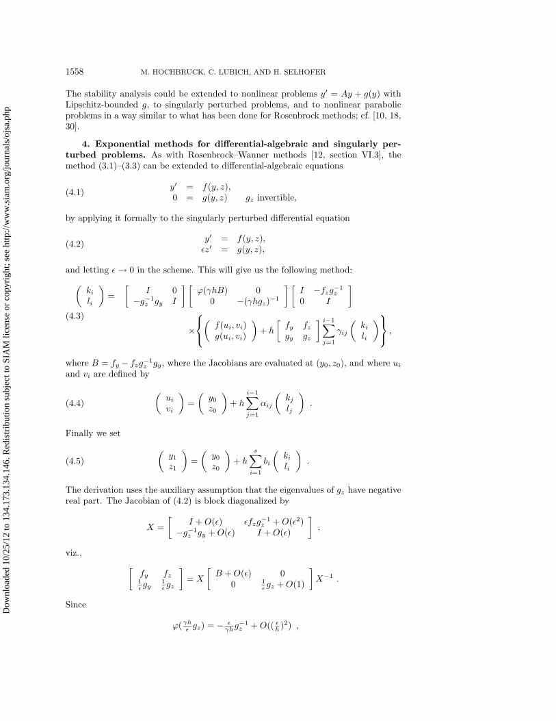
4. Exponential methods for differential-algebraic and singularly per-turbed problems. As with Rosenbrock–Wanner methods [12, section VI.3], themethod (3.1)–(3.3) can be extended to differential-algebraic equations
y′ = f(y, z),0 = g(y, z) gz invertible,
(4.1)
by applying it formally to the singularly perturbed differential equation
y′ = f(y, z),εz′ = g(y, z),
(4.2)
and letting ε→ 0 in the scheme. This will give us the following method:(kili
)=
[I 0
−g−1z gy I
] [ϕ(γhB) 0
0 −(γhgz)−1
] [I −fzg−1
z
0 I
]
×(
f(ui, vi)g(ui, vi)
)+ h
[fy fzgy gz
] i−1∑j=1
γij
(kili
) ,
(4.3)
where B = fy − fzg−1z gy, where the Jacobians are evaluated at (y0, z0), and where ui
and vi are defined by (uivi
)=
(y0
z0
)+ h
i−1∑j=1
αij
(kjlj
).(4.4)
Finally we set (y1
z1
)=
(y0
z0
)+ h
s∑i=1
bi
(kili
).(4.5)
The derivation uses the auxiliary assumption that the eigenvalues of gz have negativereal part. The Jacobian of (4.2) is block diagonalized by
X =
[I +O(ε) εfzg
−1z +O(ε2)
−g−1z gy +O(ε) I +O(ε)
],
viz., [fy fz1ε gy
1ε gz
]= X
[B +O(ε) 0
0 1ε gz +O(1)
]X−1 .
Since
ϕ(γhε gz) = − εγhg
−1z +O(( εh )2) ,
Dow
nloa
ded
10/2
5/12
to 1
34.1
73.1
34.1
46. R
edis
trib
utio
n su
bjec
t to
SIA
M li
cens
e or
cop
yrig
ht; s
ee h
ttp://
ww
w.s
iam
.org
/jour
nals
/ojs
a.ph
p
EXPONENTIAL INTEGRATORS 1559
the method (3.1)–(3.3) applied to (4.2) reads(kili
)= X
[ϕ(γhB) +O(hε) 0
0 − εγhg
−1z +O(( εh )2)
]X−1
×(
f(ui, vi)1ε g(ui, vi)
)+ h
[fy fz1ε gy
1ε gz
] i−1∑j=1
γij
(kili
) .
We note that [I 00 εI
]X−1
[I 00 1
ε I
]=
[I −fzg−1
z
0 I
]+O(ε) .
For ε→ 0, these formulas lead to the above method (4.3).Remark. The matrix B need not be computed when one uses Krylov methods
to approximate ϕ(γhB)u. Matrix–vector multiplications with B are cheap when theaction of g−1
z is inexpensive to compute. For example, this is the case in constrainedmechanical systems, cf. [12, p. 542],
q′ = v,
v′ = a,[M G(q)T
G(q) 0
](aλ
)=
(φ(q, v)ψ(q, v)
).
Here, q and v are position and velocity variables, respectively, a is acceleration, and
λ represents the Lagrange multipliers. In this system, gz corresponds to [MGGT
0 ]. Insuitable multibody formulations, linear equations with this matrix can be solved inan amount of work proportional to the dimension.
When the exponential method is exact for linear differential equations with con-stant inhomogeneity, then method (4.3)–(4.5) is exact for linear differential-algebraicequations
y′ = Fyy + Fzz + b,
0 = Gyy +Gzz + c,
with constant matrices Fy, Fz, Gy, Gz (Gz invertible) and constant vectors b, c. Apartfrom a direct calculation, this may be seen as follows: when the eigenvalues of Gz havenegative real part, the exactness is again obtained by letting ε → 0 in the singularlyperturbed problem, which is solved exactly by the method. From this case, theexactness in the general situation of invertible Gz follows by analytical continuation.
In general, the application of this scheme to differential-algebraic equations resultsin an order reduction to order 2, unless the method coefficients satisfy additionalconditions.
Theorem 4.1. The method (4.3)–(4.5) is convergent of order 3 for the differential-algebraic equation (4.1) if it satisfies the order conditions of Table 3.1 up to order 3,(3.5), and, in addition, ∑
j,k,l,m
bjωjkαklαkm = 1,(4.6)
where [ωjk] = (β + γI)−1 with β = [βjk].
Dow
nloa
ded
10/2
5/12
to 1
34.1
73.1
34.1
46. R
edis
trib
utio
n su
bjec
t to
SIA
M li
cens
e or
cop
yrig
ht; s
ee h
ttp://
ww
w.s
iam
.org
/jour
nals
/ojs
a.ph
p
1560 M. HOCHBRUCK, C. LUBICH, AND H. SELHOFER
The additional order condition is the same as for Rosenbrock methods applied to(4.1) [12, p. 446]. Instead of giving a cumbersome formal proof of the theorem, wemake the reappearance of condition (4.6) for exponential methods plausible as follows:similar to the order conditions of section 3, the differential-algebraic order conditionsare also of the same form as for Rosenbrock methods but possibly with differentright-hand sides involving γ. We know that the theorem is valid for ϕ(z) = 1/(1− z).The appearance of the ωjk is related only to the term (γhgz)
−1 in (4.3), which isindependent of ϕ. The terms αjk are also unrelated to ϕ(γhB). Therefore, thecondition remains the same as for Rosenbrock methods.
The differential-algebraic order condition (4.6) is important not only for differential-algebraic systems but also for stiff differential equations. For example, the third-ordererror bound of Rosenbrock methods for singularly perturbed problems (4.2) in The-orem 1 (case r = 3) of [10] can be shown to be valid also for exponential methods.
5. Construction of fourth-order methods.
5.1. Reduced methods. We recall that one step of the exponential methodevaluated in the form (3.1)–(3.3) contains s multiplications of ϕ(γhA) with a vector.Since this vector is different in each of these s steps, the approximation with a Krylovsubspace method requires the construction of bases of s Krylov spaces with respectto the same matrix A but with different vectors. This turns out to be prohibitivelyexpensive. One may think of exploiting techniques for solving linear systems withmultiple right-hand sides [25, 27], but in our experiments the savings achieved wereminor. Therefore, we will present an alternative formulation of the method.
A key point for the construction of efficient methods is that one can computeϕ(jz), j = 2, 3, . . ., recursively from ϕ(z):
ϕ(2z) =(
12zϕ(z) + 1
)ϕ(z),
ϕ(3z) = 23 (zϕ(z) + 1)ϕ(2z) + 1
3ϕ(z),(5.1)
ϕ(4z) = · · · .
Once we have computed ϕ(γhA), we can thus compute ϕ(jγhA)v for any integerj > 1 with the expense of matrix–vector multiplications.
The recurrence (5.1) is equally useful for the more interesting case where ϕ(jγhA)vis approximated by Krylov methods. The Krylov subspace approximation is of theform
ϕ(τA)v ≈ Vmϕ(τHm)e1 · ‖v‖2,(5.2)
where Vm = [v1, . . . , vm] is the matrix containing the Arnoldi (or Lanczos) basis ofthe mth Krylov subspace with respect to A and v, and Hm is the orthogonal (oblique)projection of A to the mth Krylov subspace, which is an m ×m upper Hessenberg(block tridiagonal, respectively) matrix. Further, e1 is the first m-dimensional unitvector.
The iteration number m is typically very small compared with the dimension ofthe matrix A, so that the matrix ϕ(γhHm) can be computed quite cheaply (see section6 for details). Then the recurrence (5.1) can be used to compute ϕ(jγhHm)e1 byperforming matrix–vector multiplications with the small matrices Hm and ϕ(γhHm).If we denote the identity matrix of dimension m by Im, thenD
ownl
oade
d 10
/25/
12 to
134
.173
.134
.146
. Red
istr
ibut
ion
subj
ect t
o SI
AM
lice
nse
or c
opyr
ight
; see
http
://w
ww
.sia
m.o
rg/jo
urna
ls/o
jsa.
php
EXPONENTIAL INTEGRATORS 1561
ϕ(2τA)v ≈ Vmϕ(2τHm)e1‖v‖2
= Vm(
12τHmϕ(τHm) + Im
)ϕ(τHm)e1‖v‖2,
ϕ(3τA)v ≈ Vm(
23 (τHmϕ(τHm) + Im)ϕ(2τHm) + 1
3ϕ(τHm))e1‖v‖2 .
We can exploit the recurrences (5.1) by reformulating the method. For this weintroduce auxiliary vectors
di = f(ui)− f(y0)− hAs∑
j=1
αijkj .(5.3)
Note that for A = f ′(y0), this corresponds to a first-degree Taylor expansion of f aty0. Hence the vectors di are usually small in norm and would vanish for linear f .With (3.4) and (5.3) we have
ki = k1 + ϕ(γhA)di + ϕ(γhA)hAs∑
j=1
βijkj .
Because of (5.1) we can choose βkl such that for γ = 1/n and i = 1, . . . , n,
ki = ϕ(iγhA)f(y0),knj+i = k1 + ϕ(iγhA)dnj+i, j ≥ 1.
(5.4)
All the coefficients βkl are uniquely determined by (5.4). In order to apply the recur-rence formulas (5.1) in (5.4) we further choose
αnj+i,l = αnj+1,l, i = 1, . . . , n, j, l ≥ 1,
which gives
unj+i = unj+1,dnj+i = dnj+1,
i = 1, . . . , n, j ≥ 1.
This reduces the number of f -evaluations and of evaluations of ϕ(γhA) by a factor ofn compared with the general scheme (3.1)–(3.3). This is particularly important whenthis reduced method is combined with a Krylov process for approximating ϕ(γhA)vsince in this case we need to compute a basis of a new Krylov space only at everynth intermediate step. Moreover, since the vectors di are usually small in norm, theKrylov approximation of ϕ(iγhA)dnj+1 (j ≥ 1) typically takes only a few iterationsto achieve the required accuracy. The cost for building up the Krylov space of A withrespect to the vector f(y0) thus dominates the computational cost.
We note finally that we can reorganize the computations in (5.4) as
ki = ki = ϕ( inhA)f(y0),
knj+i = knj+i − k1 = ϕ( inhA)dnj+1,(5.5)
for i = 1, . . . , n and j ≥ 1, and we can use the values kl in (3.2) and (3.3) withappropriately modified weights:
αk,l =
{αk,l +
∑m>n αk,m, l = 1,
αk,l, l > 1,
and
bl =
{bl +
∑m>n bm, l = 1,
bl, l > 1 .(5.6)
Dow
nloa
ded
10/2
5/12
to 1
34.1
73.1
34.1
46. R
edis
trib
utio
n su
bjec
t to
SIA
M li
cens
e or
cop
yrig
ht; s
ee h
ttp://
ww
w.s
iam
.org
/jour
nals
/ojs
a.ph
p
1562 M. HOCHBRUCK, C. LUBICH, AND H. SELHOFER
5.2. Methods of order 4. Next we show that the reduced scheme proposedabove still allows the construction of higher-order methods. Here, we concentrate onγ = 1/2 and γ = 1/3 and start with a three-stage method for γ = 1/2 that uses twofunction evaluations per step. The parameters βkl satisfying (5.4) are given by
β =
0 0 01/4 0 0
0 0 0
.To fulfill the conditions for order 4, there remain two free parameters α3,1, α3,2 and theweights bj , j = 1, . . . , 4. The order conditions from Table 3.1 have a unique solution
α =
0 0 00 0 0
3/8 3/8 0
, bT = (−16/27, 1, 16/27) .
This yields the scheme
k1 = ϕ( 12hA)f(y0),
k2 = ϕ(hA)f(y0),
w3 = 38 (k1 + k2),
u3 = y0 + hw3,
d3 = f(u3)− f(y0)− hAw3,
k3 = ϕ( 12hA)d3,
y1 = y0 + h(k2 + 1627k3) .
(5.7)
On k3 we have omitted the tilde corresponding to (5.5). This method is of order 4and is exact for linear differential equations (1.2). However, it is only of first orderwhen used with inexact Jacobian and of second order when applied to differential-algebraic equations. Moreover, it is impossible to construct an embedded methodof order 3, which makes it hard to perform a reliable estimation of local errors forstep-size control. The only cheap variant is to use the exponential Euler method (2.1),which is only of order 2 and thus tends to overestimate the local error.
The method (5.7) with embedded (2.1), however, is of interest as a very econom-ical method in situations where the time step is not restricted by accuracy but onlyby the convergence of the Krylov process for computing ϕ(hA)f(y0). We note that k3
is usually well approximated in a low-dimensional Krylov space, because d3 is oftenmuch smaller in norm than f(y0).
A more sophisticated method can be constructed with γ = 1/3 and s = 7, usingthree function evaluations per step. The parameters for (5.4) are given by
β =
0 01/6 01/9 2/9 0
0 0 0 0−1/6 0 0 1/6 0−1/3 0 0 1/9 2/9 0
0 0 0 0 0 0 0
.
With these parameters βkl, all the order conditions (3.5) for linear problems aresatisfied automatically for n ≥ 4.
Dow
nloa
ded
10/2
5/12
to 1
34.1
73.1
34.1
46. R
edis
trib
utio
n su
bjec
t to
SIA
M li
cens
e or
cop
yrig
ht; s
ee h
ttp://
ww
w.s
iam
.org
/jour
nals
/ojs
a.ph
p
EXPONENTIAL INTEGRATORS 1563
For our method we choose to evaluate the function f at both end points and atthe middle of the time interval; i.e.,
3∑j=1
α4,j :=1
2,
6∑j=1
α7,j := 1 .
The solution is obtained by first solving the order condition up to order 4 from Ta-ble 3.1. The equations for f ′′(f, f) and f ′f immediately yield b3 = 1 and b2 = 0.Next the conditions for f ′f ′f , f ′′′(f, f, f), f ′f ′′(f, f), and (4.6) result in a linearsystem with four equations for the unknowns bj , j = 4, . . . , 7. This system hasthe unique solution b4 = b6 = 1, b5 = −4/3, b7 = 1/6, which also satisfies thesecond-order W-condition. From the equation for f we obtain b1 = −5/6. It re-mains to fulfill the equation for f ′′(f ′f, f), and further we satisfy the third-orderW-condition for f ′f ′f in order to obtain order 3 when the approximation to the Jaco-bian is O(h) close to the true Jacobian. This yields α4,2 = 5/4−α4,3− 1/2α7,2−α7,3
and α7,4 = −α7,5 − α7,6 + 2. We still have some freedom so that we can solve thefifth-order conditions for f ′′′(f ′f, f, f) and f ′′(f ′f ′f, f). This gives α7,2 = 2/5+4α4,3
and α7,3 = −2α4,3 + 13/20. Since no other fifth-order conditions can be satisfied, wenow minimize
3∑j=1
α24,j +
6∑j=1
α27,j ,
which yields α4,3 = −37/300 and α7,5 = α7,6 = 2/3.This construction gives us the following method:
k1 = ϕ( 13hA)f(y0),
k2 = ϕ( 23hA)f(y0),
k3 = ϕ(hA)f(y0),
w4 = − 7300k1 + 97
150k2 − 37300k3,
u4 = y0 + hw4,
d4 = f(u4)− f(y0)− hAw4,
k4 = ϕ( 13hA)d4,(5.8)
k5 = ϕ( 23hA)d4,
k6 = ϕ(hA)d4,
w7 = 59300k1 − 7
75k2 + 269300k3 + 2
3 (k4 + k5 + k6),
u7 = y0 + hw7,
d7 = f(u7)− f(y0)− hAw7,
k7 = ϕ( 13hA)d7,
y1 = y0 + h(k3 + k4 − 43k5 + k6 + 1
6k7).
Again, we have omitted the tilde on k4, . . . , k7 as used in (5.5). We summarize theproperties of this method in a theorem.
Theorem 5.1. The scheme (5.8) is of order 4 for differential equations (1.1) andis exact for linear differential equations (1.2). It converges to order 3 for differential-algebraic equations (4.1) and to smooth solutions of singularly perturbed problems (4.2)uniformly for ε ≤ h2. For differential equations (1.1), it is of second order when used
Dow
nloa
ded
10/2
5/12
to 1
34.1
73.1
34.1
46. R
edis
trib
utio
n su
bjec
t to
SIA
M li
cens
e or
cop
yrig
ht; s
ee h
ttp://
ww
w.s
iam
.org
/jour
nals
/ojs
a.ph
p
1564 M. HOCHBRUCK, C. LUBICH, AND H. SELHOFER
with inexact Jacobian and is of order 3 when the approximation to the Jacobian isO(h) close to the true Jacobian.
The method satisfies three of the order-5 conditions. The residuals of the otherorder-5 conditions appear to be rather small, the largest one being 0.1.
Although the scheme (5.8) is a seven-stage method, it requires only three functionevaluations. When using Krylov approximations, the computational cost is dominatedby computing k1. As discussed before, the reason is that k2, k3, k5, and k6 can becomputed recursively from (5.1) or the more stable recurrence (6.2) below and thatk4 to k7 are typically well approximated in very low dimensional Krylov subspaces,because d4 and d7 are usually much smaller in norm than f(y0). For these reasons,and because of its superior theoretical properties, we prefer (5.8) to a “standard”three-stage fourth-order scheme of type (3.1)–(3.3).
5.3. Embedded methods. We have constructed two embedded methods withdifferent properties for the scheme (5.8). The first one is of order 3 for differentialequations (1.1) and differential-algebraic equations (4.1) and is exact for linear equa-tions (1.2). Solving the third-order conditions of Table 3.1 and condition (4.6) andchoosing b6 = b7 = 1/2 gives the embedded scheme
y1 = y0 + h(k3 − 12k4 − 2
3k5 + 12k6 + 1
2k7) .(5.9)
This method does not satisfy the fourth-order conditions, except for f ′f ′f ′f . It is,however, only of order 1 as a W-method, i.e., when used with inexact Jacobian.
The second embedded method is of order 2 as a W-method. It is not exact forlinear differential equations (1.2), and it does not satisfy the third-order conditions ofTable 3.1. It reads
y1 = y0 + h(−k1 + 2k2 − k4 + k7).(5.10)
5.4. Dense output. Similar to the Runge–Kutta and Rosenbrock methods, acontinuous numerical solution y(t0 + θh) is defined via
y1(θ) = y0 + hs∑
i=1
bi(θ)ki
with polynomials bi satisfying bi(0) = 0 and bi(1) = bi. This approximation is oforder p, i.e.,
y(t0 + θh)− y1(θ) = O(hp+1) ,
iff
s∑i=1
bi(θ)Φi(τ) = θρPτ (γ)
for all elementary differentials τ of order ρ ≤ p; see [12, p. 452].For the three-stage method (5.7) a continuous numerical solution of order 3 is
given by
b1(θ) = θ(1− θ − 1627θ
2),
b2(θ) = θ2,
b3(θ) = 1627θ
3.
Dow
nloa
ded
10/2
5/12
to 1
34.1
73.1
34.1
46. R
edis
trib
utio
n su
bjec
t to
SIA
M li
cens
e or
cop
yrig
ht; s
ee h
ttp://
ww
w.s
iam
.org
/jour
nals
/ojs
a.ph
p
EXPONENTIAL INTEGRATORS 1565
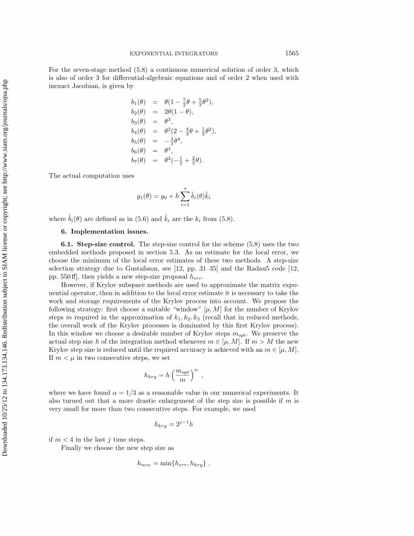
For the seven-stage method (5.8) a continuous numerical solution of order 3, whichis also of order 3 for differential-algebraic equations and of order 2 when used withinexact Jacobian, is given by
b1(θ) = θ(1− 72θ + 5
3θ2),
b2(θ) = 2θ(1− θ),
b3(θ) = θ3,
b4(θ) = θ2(2− 43θ + 1
3θ2),
b5(θ) = − 43θ
4,
b6(θ) = θ4,
b7(θ) = θ2(− 12 + 2
3θ).
The actual computation uses
y1(θ) = y0 + hs∑
i=1
bi(θ)ki
where bi(θ) are defined as in (5.6) and ki are the ki from (5.8).
6. Implementation issues.
6.1. Step-size control. The step-size control for the scheme (5.8) uses the twoembedded methods proposed in section 5.3. As an estimate for the local error, wechoose the minimum of the local error estimates of these two methods. A step-sizeselection strategy due to Gustafsson, see [12, pp. 31–35] and the Radau5 code [12,pp. 550 ff], then yields a new step-size proposal herr.
However, if Krylov subspace methods are used to approximate the matrix expo-nential operator, then in addition to the local error estimate it is necessary to take thework and storage requirements of the Krylov process into account. We propose thefollowing strategy: first choose a suitable “window” [µ,M ] for the number of Krylovsteps m required in the approximation of k1, k2, k3 (recall that in reduced methods,the overall work of the Krylov processes is dominated by this first Krylov process).In this window we choose a desirable number of Krylov steps mopt. We preserve theactual step size h of the integration method whenever m ∈ [µ,M ]. If m > M the newKrylov step size is reduced until the required accuracy is achieved with an m ∈ [µ,M ].If m < µ in two consecutive steps, we set
hkry = h(mopt
m
)α,
where we have found α = 1/3 as a reasonable value in our numerical experiments. Italso turned out that a more drastic enlargement of the step size is possible if m isvery small for more than two consecutive steps. For example, we used
hkry = 2j−1h
if m < 4 in the last j time steps.Finally we choose the new step size as
hnew = min{herr, hkry} .
Dow
nloa
ded
10/2
5/12
to 1
34.1
73.1
34.1
46. R
edis
trib
utio
n su
bjec
t to
SIA
M li
cens
e or
cop
yrig
ht; s
ee h
ttp://
ww
w.s
iam
.org
/jour
nals
/ojs
a.ph
p
1566 M. HOCHBRUCK, C. LUBICH, AND H. SELHOFER
6.2. Savings from previous steps. The scheme may reuse the Jacobian of aprevious time step as an approximation to the actual Jacobian. This is done if thelocal error of the embedded method (5.10) is acceptable and in addition hkry ≤ herr;i.e., the step size is determined by the Krylov process.
Further savings can be achieved if the Jacobian A and the step size h are thesame as in the previous time step. We then write
If f(yn) is close to f(yn−1), then the initial vector for the Krylov process is small innorm and thus the Krylov process becomes less expensive.
6.3. Stopping criterion for the Krylov method. We need to decide whenthe Krylov approximation (5.2) is to be considered sufficiently accurate. Since exacterrors are inaccessible, the stopping criterion in the iterative solution of linear systems(λI − τA)x = v is usually based on the residual
rm(λ) = v − (λI − τA)xm
instead of the error of the mth iterate
em(λ) = xm − x .
For Galerkin-type methods like FOM and BiCG, the residual vectors can be computedfrom
rm(λ) = ‖v‖2 · τhm+1,m [(λI − τHm)−1]m,1 · vm+1 ,
where hm+1,m is the (m+1,m)-entry of Hm+1, and [ · ]m,1 denotes the (m, 1)-entry ofa matrix. Using Cauchy’s integral formula, the error of the mth Krylov approximationto ϕ(τA)v can be written as
εm = Vmϕ(τHm)e1 · ‖v‖2 − ϕ(τA)v =1
2πi
∫Γ
ϕ(λ) em(λ) dλ ,
where Γ is a contour enclosing the eigenvalues of τA and τHm; cf. [13]. Thus, theerror εm can be interpreted as a linear combination of errors em(λ) of linear systems.Replacing em(λ) by rm(λ) in this formula, we get a generalized residual
ρm =1
2πi
∫Γ
ϕ(λ) rm(λ) dλ = ‖v‖2 · τhm+1,m [ϕ(τHm)]m,1 vm+1 ,
which can be computed at no additional cost. This suggests using ρm instead of theunknown error εm in the stopping criterion. The use of ρm was also proposed by Saad[26], who used a different derivation that is plausible only for small ‖τA‖.
In the scheme (5.8), the Krylov approximations to kj are multiplied by the stepsize h. It is therefore reasonable to stop the iteration if
h ‖ρm‖tol < 1 ,(6.1)
where ‖ · ‖tol is the weighted norm used in the integrator
‖d‖tol =
(1
N
N∑i=1
(di/wi)2
)1/2
Dow
nloa
ded
10/2
5/12
to 1
34.1
73.1
34.1
46. R
edis
trib
utio
n su
bjec
t to
SIA
M li
cens
e or
cop
yrig
ht; s
ee h
ttp://
ww
w.s
iam
.org
/jour
nals
/ojs
a.ph
p
EXPONENTIAL INTEGRATORS 1567
with wi = atoli+max(|yn,i|, |yn−1,i|) · rtol, where atoli and rtol are the given absoluteand relative error tolerances.
In our numerical experiments we found that (6.1) is on the safe side but is some-times rather pessimistic. Then it may pay off to apply an idea attributed to Shampinein [12, p. 134], which consists in using a smoothed residual (I − τA)−1ρm instead ofthe true residual. Since solving a linear system with coefficient matrix (I − τA)is prohibitively expensive when A is large, one can perform a smoothing in the m-dimensional subspace and use
instead of (6.1) for m ≥ 5, say. For smaller m, this criterion may be overly optimisticwhen τA has large norm.
6.4. Computation of ϕ(τHm). To reduce the computational costs, we evalu-ate ϕ(τHm) only whenm figures in an index sequence, e.g., m ∈ {1, 2, 3, 4, 6, 8, 11, 15, 20,27, 36, 48}. This sequence is chosen such that the computation of ϕ(τHm) is ap-proximately as expensive as the total of the previously computed ϕ(τHj), since thecomputation of ϕ(τHm) requires O(m3) arithmetic operations.
If A is Hermitian, then Hm is Hermitian tridiagonal. In this case, one can simplydiagonalize Hm.
In the non-Hermitian case, we suggest using a Pade approximation similar to thethird method described in [19] to compute the matrix exponential. Here the matrixis first scaled by a factor of 2−k such that ‖2−kτHm‖ < 1/2. Then we evaluate the(6, 6) Pade approximation to ϕ(z) for the scaled matrix:
ϕ(z) =1 + 1
26z + 5156z
2 + 1858z
3 + 15720z
4 + 1205920z
5 + 18648640z
6
1− 613z + 5
52z2 − 5
429z3 + 1
1144z4 − 1
25740z5 + 1
1235520z6
+O(z13) .
Next ϕ(τHm) is computed recursively from ϕ(2−kτHm) by applying the followingcoupled recurrences:
ϕ(2z) = 12 (ez + 1)ϕ(z),
e2z = ezez .(6.2)
This recurrence is stable for all z in the left half-plane, whereas (5.1) becomes unstablefor large |z| because of the multiplication with z.
Alternatively, in the non-Hermitian case, one can use a formula due to Saad [26,section 2.3]:
exp
[τHm e1
0 0
]=
[exp(τHm) ϕ(τHm)e1
0 1
].
This appears favorable when the dimension m is not too small.
7. Numerical experiments. We have implemented the method (5.8) with (andwithout) Krylov approximations in a Matlab code exp4. The program is written inthe format used in the Matlab ODE suite [28], which is available via anonymous ftpon ftp.mathworks.com in the pub/mathworks/toolbox/matlab/funfun directory. Thecode exp4 can be obtained from na.uni-tuebingen.de in the pub/codes/exp4 directory.A C version of exp4 is also available from this ftp site.
Dow
nloa
ded
10/2
5/12
to 1
34.1
73.1
34.1
46. R
edis
trib
utio
n su
bjec
t to
SIA
M li
cens
e or
cop
yrig
ht; s
ee h
ttp://
ww
w.s
iam
.org
/jour
nals
/ojs
a.ph
p
1568 M. HOCHBRUCK, C. LUBICH, AND H. SELHOFER
7.1. A reaction-diffusion equation with nonstiff chemical reaction: TheBrusselator. To illustrate the behavior of the exponential integrator with Krylovapproximations to ϕ(γhA)v in the transition from a nonstiff to a stiff problem, wehave chosen the two-dimensional Brusselator [11, pp. 248 ff]:
∂u
∂t= 1 + u2v − 4u+ α∆u,
∂v
∂t= 3u− u2v + α∆v
for 0 ≤ x, y ≤ 1 together with Neumann boundary conditions
∂u
∂n= 0,
∂v
∂n= 0
and initial conditions v(x, y, 0) = 0 and u(x, y, 0) taken from Matlab’s peak function
The Laplacian is discretized on a uniform 100×100 grid by central differences, so thatthe dimension of the resulting ODE problem is 20, 000. The eigenvalues of the dis-cretized Laplacian lie between −80, 000 and zero. We present numerical experimentswith three different values of the diffusion coefficient α = 2 · 10−4, 2 · 10−3, 2 · 10−2,which mark the transition from a nonstiff to a stiff problem.
In Figs. 7.1–7.3 we show work-precision diagrams for our exponential integratorexp4 and for the explicit Runge–Kutta integrator ode45 from the Matlab ODEsuite [28], which is based on a fifth-order method of Dormand and Prince [3]. Thevertical axis shows the error at the end point t = 1; the horizontal axis gives thenumber of flops. The markers × for exp4 and ◦ for ode45 correspond to the errortolerances atol=rtol= 10−3, 10−3.5, . . . , 10−7.5. While the computational work of thenonstiff integrator increases drastically with growing α, the performance of exp4 isconsiderably less affected.
7.2. A reaction-diffusion equation with stiff chemistry: The Robertsonexample. The following example shows the behavior of the exponential integratorfor a very stiff problem. We consider the Robertson reaction [12, pp. 3f] with one-dimensional diffusion:
ut = −0.04u+ 104vw + αuxx,
vt = 0.04u− 104vw − 3 · 107v2 + αvxx,
wt = 3 · 107v2 + αwxx
for 0 ≤ x ≤ 1, 0 ≤ t ≤ 400 together with Neumann boundary conditions ux = vx =wx = 0 at x = 0, 1 and initial values
u(x, 0) = 1 + sin(2πx), v(x, 0) = w(x, 0) = 0 .
The diffusion coefficient is chosen as α = 2 · 10−2. The second spatial derivativeis discretized on a uniform grid with 30 grid points. In this problem, the stiffnessoriginates from the reaction terms. We have chosen such a small problem becausewe intend to illustrate the influence of the Krylov approximation procedure to theperformance of the integrator. In Fig. 7.4 we show the step sizes as a function of time
Dow
nloa
ded
10/2
5/12
to 1
34.1
73.1
34.1
46. R
edis
trib
utio
n su
bjec
t to
SIA
M li
cens
e or
cop
yrig
ht; s
ee h
ttp://
ww
w.s
iam
.org
/jour
nals
/ojs
a.ph
p
EXPONENTIAL INTEGRATORS 1569
107
108
109
1010
10−9
10−8
10−7
10−6
10−5
10−4
10−3
10−2
ode45
exp4
error
flops
Fig. 7.1. Brusselator for α = 2 · 10−4.
107
108
109
1010
10−9
10−8
10−7
10−6
10−5
10−4
10−3
10−2
flops
errorexp4
ode45
Fig. 7.2. Brusselator for α = 2 · 10−3.
107
108
109
1010
10−9
10−8
10−7
10−6
10−5
10−4
10−3
10−2
ode45exp4
error
flops
Fig. 7.3. Brusselator for α = 2 · 10−2.
Dow
nloa
ded
10/2
5/12
to 1
34.1
73.1
34.1
46. R
edis
trib
utio
n su
bjec
t to
SIA
M li
cens
e or
cop
yrig
ht; s
ee h
ttp://
ww
w.s
iam
.org
/jour
nals
/ojs
a.ph
p
1570 M. HOCHBRUCK, C. LUBICH, AND H. SELHOFER
10−3
10−2
10−1
100
101
102
10−4
10−3
10−2
10−1
100
101
102
ode15s
ode45
exp4 without Krylov
exp4 with Krylov
step size
time
Fig. 7.4. Step sizes versus time for the Robertson example.
in a double logarithmic scale with and without Krylov approximation of ϕ(γhA)v. Asthis example has only dimension 90, ϕ(γhA) can here be computed by diagonalization.For comparison, we also show the step size of the explicit integrator ode45 and thestiff integrator ode15s from the Matlab ODE suite [28], which uses a variant of abackward differentiation formula (BDF) method. All the methods have been run withthe same tolerances atol=rtol= 10−6. It is seen that in this example the step size isalways limited by the Krylov process. The step-size restriction does not appear verysevere on the considered time interval. Similar step-size sequences are obtained forthe Krylov-approximated exponential method for higher-dimensional versions of theproblem. However, the limits of the Krylov approach show up when the integrationis continued for very long length’s of time. There, the step size remains essentiallyon the level seen at the rightmost part of Fig. 7.4. It has been observed that thisbehavior is largely due to roundoff error effects.
7.3. A Schrodinger equation with time-dependent potential. As an ex-ample of a problem whose Jacobian has large imaginary eigenvalues we consider,following [23], the one-dimensional Schrodinger equation for ψ = ψ(x, t):
i∂ψ
∂t= H(x, t)ψ
with the Hamiltonian
H(x, t) = −1
2
∂2
∂x2+ κ
x2
2+ µ sin2(t)x .
This equation models an atom/molecule interacting with a high intensity CW laser.The parameter values used were κ = 10 and µ = 100. The initial value was ψ(x, 0) =
e−√κx2/2, which corresponds to the eigenstate of the unforced harmonic oscillator
Dow
nloa
ded
10/2
5/12
to 1
34.1
73.1
34.1
46. R
edis
trib
utio
n su
bjec
t to
SIA
M li
cens
e or
cop
yrig
ht; s
ee h
ttp://
ww
w.s
iam
.org
/jour
nals
/ojs
a.ph
p
EXPONENTIAL INTEGRATORS 1571
to the lowest energy level. Semidiscretization in space is done by a pseudospectralmethod with N = 512 Fourier modes on the space interval x ∈ [−a, a] for a = 10with periodic boundary conditions. This leads to the nonautonomous linear systemof differential equations for y = (y1, . . . , yN )T ,
y′ = −i(− 1
2F−1N D2FN + diag
(κx2j
2 + µ sin2(t)xj
))y .
Here yj(t) is an approximation to ψ(xj , t) at xj = −a + j 2aN , FN is the discrete
Fourier-transform operator, and
D = iπa diag(0, 1, . . . , N2 − 1,−N2 ,−N
2 + 1, . . . ,−1) .
The Jacobian is full, but matrix–vector multiplications are obtained with O(N logN)flops using FFT. In Fig. 7.5 we show the work-precision diagram at t = 1 forexp4, for the standard nonstiff and stiff solvers ode45 and ode15s from the Mat-lab ODE suite, and for a Matlab implementation of Hairer and Wanner’s [12]Radau5 implicit Runge–Kutta code. The codes were used with tolerances atol=rtol=10−3, 10−4, . . . , 10−8. The surprisingly good behavior of the stiff integrators ode15s
and radau5 is due to the following matrix-free implementation: in the simplifiedNewton iterations the Jacobian was approximated by i/2F−1
N D2FN , so that the lin-ear systems could be solved in O(N logN) operations using FFT. Therefore, thecomputational cost per time step was essentially the same as for an explicit method.Using the full Jacobian would make the implicit methods completely inefficient for thisproblem. We note, however, that the performance of the versions with the simplifiedJacobian deteriorates when the parameters κ and µ increase.
The exponential code exp4 is clearly superior to the explicit integrator ode45.For accuracy requirements more stringent than 10−4, Fig. 7.5 shows an advantage forexp4 also with respect to the implicit methods in their optimized versions discussedabove. This stems from the fact that exp4 is able to take much larger time steps thanthe other integrators.
In computations with Schrodinger equations with time-independent Hamiltonian,the use of Chebyshev approximations to the matrix exponential operator is very popu-lar [16]. We therefore also implemented a version of exp4 where the Arnoldi process isreplaced by a Chebyshev approximation. In our numerical experiments the Chebyshevversion needed about twice as many flops as the Arnoldi-based implementation.
(We thank S. Gray for pointing out references [16] and [23].)
8. Conclusions and perspectives. In this paper we have introduced new in-tegration methods which use matrix–vector multiplications with the exponential ofthe Jacobian. In particular, we have studied Rosenbrock-like exponential methods.Since a straightforward implementation of these methods is computationally expen-sive, we have identified a subclass of “reduced” methods which are reformulated suchthat they allow for an efficient implementation. Two promising fourth-order methods,which are exact for linear constant-coefficient problems, have been given in formulas(5.7) and (5.8). The method (5.8), which offers superior properties at slightly highercost per time step, has been implemented with Krylov subspace approximations tothe matrix exponential operator in a code exp4. This implementation requires onlyfunction evaluations and matrix–vector multiplications with the Jacobian.
Numerical experiments and theoretical considerations indicate that exponentialintegrators are highly competitive for the following problem classes of large systemsof initial value problems.
Dow
nloa
ded
10/2
5/12
to 1
34.1
73.1
34.1
46. R
edis
trib
utio
n su
bjec
t to
SIA
M li
cens
e or
cop
yrig
ht; s
ee h
ttp://
ww
w.s
iam
.org
/jour
nals
/ojs
a.ph
p
1572 M. HOCHBRUCK, C. LUBICH, AND H. SELHOFER
108
109
1010
10−8
10−7
10−6
10−5
10−4
10−3
10−2
10−1
ode15s
ode45
radau5
exp4
error
flops
Fig. 7.5. Work-precision diagram for the Schrodinger equation.
Mildly stiff problems (e.g., reaction-convection-diffusion problems with nonstiffreaction terms). The most efficient traditional methods are explicit integrators whichare used despite stability restrictions of the step size. For the special case where theeigenvalues of the Jacobian are on the negative real axis, the high-stage Runge–Kutta–Chebyshev methods of van der Houwen and Sommeijer in [14, 31] are known to be verysuccessful. Here the theory in [5, 13] and [31] tells us that the number of necessarymatrix–vector multiplications with the Jacobian in Krylov iterations for exponentialmethods and the number of function evaluations in Runge–Kutta–Chebyshev methodsneeded to attain stability are both of the magnitude of
√h‖A‖. However, the Krylov
methods take advantage of clustered eigenvalues and of vectors with small componentsin some eigendirections. There is no restriction to problems with eigenvalues near thereal axis for the exponential methods with Krylov approximations, and much largertime steps than with standard explicit Runge–Kutta methods (such as the Dormand–Prince methods) can be taken.
Stiff problems (e.g., reaction-diffusion problems with stiff reaction terms). Forhigh-dimensional systems, the standard approach is to use implicit methods (such asBDF or Radau) where the linear systems are solved iteratively with the help of ahopefully good and cheap preconditioner. If and only if an efficient preconditioner isavailable, those methods are clearly favorable over the exponential methods proposedhere, since it is not known how to precondition the iterative computation of thematrix exponential operator. Due to the superlinear error reduction of the Krylovapproximations to the matrix exponential, exponential methods are often competitiveeven without a preconditioner. We hope that future developments will allow us toeffectively use ideas of preconditioning in the computation of the exponentials andhence further enlarge the range of stiff problems on which exponential methods areefficiently applicable.D
ownl
oade
d 10
/25/
12 to
134
.173
.134
.146
. Red
istr
ibut
ion
subj
ect t
o SI
AM
lice
nse
or c
opyr
ight
; see
http
://w
ww
.sia
m.o
rg/jo
urna
ls/o
jsa.
php
EXPONENTIAL INTEGRATORS 1573
Highly oscillatory problems (e.g., wave equations, Schrodinger equations, elasto-dynamics, and oscillatory electric circuits). Here the proposed exponential methodsare able to resolve high frequencies to the required error tolerance without the severetime-step restrictions of standard schemes. Time-step restrictions of an often mildertype still occur because of nonlinear effects and because of limitations of the iterationnumber in the Krylov process. The latter are less severe when the eigenvalues ofthe Jacobian are clustered. The good resolution of high frequencies with exponentialmethods is in contrast to usual implicit integrators used with large time steps, whicheither damp high frequencies or map them to one and the same frequency (or nearlyso) in the discretization.
It will be interesting to see how the new methods perform in real-life scientificproblems.
REFERENCES
[1] J. Carroll, Sufficient conditions for uniformly second-order convergent schemes for stiffinitial-value problems, Comput. Math. Appl., 24 (1992), pp. 105–116.
[2] G. Denk, A new efficient numerical integration scheme for highly oscillatory electric circuits,Internat. Ser. Numer. Math. 117, Birkhauser, Basel, 1994, pp. 1–15.
[3] J. R. Dormand and P. J. Prince, A family of embedded Runge-Kutta formulae, J. Comput.Appl. Math., 6 (1980), pp. 19–26.
[4] V. L. Druskin and L. A. Knizhnerman, Error bounds in the simple Lanczos procedure forcomputing functions of symmetric matrices and eigenvalues, Comput. Math. Math. Phys.,7 (1991), pp. 20–30.
[5] V. L. Druskin and L. A. Knizhnerman, Krylov subspace approximations of eigenpairs andmatrix functions in exact and computer arithmetic, Numer. Linear Algebra Appl., 2 (1995),pp. 205–217.
[6] W. S. Edwards, L. S. Tuckerman, R. A. Friesner, and D. C. Sorensen, Krylov methodsfor the incompressible Navier-Stokes equations, J. Comput. Phys., 110 (1994), pp. 82–102.
[7] A. Friedli, Verallgemeinerte Runge-Kutta Verfahren zur Losung steifer Differentialgleichun-gen, Lecture Notes in Mathematics 631, Springer-Verlag, Berlin, 1978, pp. 35–50.
[8] R. A. Friesner, L. S. Tuckerman, B. C. Dornblaser, and T. V. Russo, A method ofexponential propagation of large systems of stiff nonlinear differential equations, J. Sci.Comput., 4 (1989), pp. 327–354.
[9] E. Gallopoulos and Y. Saad, Efficient solution of parabolic equations by Krylov approxima-tion methods, SIAM J. Sci. Statist. Comput., 13 (1992), pp. 1236–1264.
[10] E. Hairer, Ch. Lubich, and M. Roche, Error of Rosenbrock methods for stiff problems studiedvia differential algebraic equations, BIT, 29 (1989), pp. 77–90.
[11] E. Hairer, S. P. Nørsett, and G. Wanner, Solving Ordinary Differential Equations I, 2nded., Springer-Verlag, Berlin, 1993.
[12] E. Hairer and G. Wanner, Solving Ordinary Differential Equations II, 2nd ed., Springer-Verlag, Berlin, 1996.
[13] M. Hochbruck and Ch. Lubich, On Krylov subspace approximations to the matrix exponentialoperator, SIAM J. Numer. Anal., 34 (1997), pp. 1911–1925.
[14] P. J. van der Houwen and B. P. Sommeijer, On the internal stability of explicit m-stageRunge-Kutta methods for large values of m, Z. Angew. Math. Mech., 60 (1980), pp. 479–485.
[15] P. Kaps and A. Ostermann, Rosenbrock methods using few LU-decompositions, IMA J. Nu-mer. Anal., 9 (1989), pp. 15–27.
[16] R. Kosloff, Propagation methods for quantum molecular dynamics, Ann. Rev. Phys. Chem.,45 (1994), pp. 145–178.
[17] J. D. Lawson, Generalized Runge-Kutta processes for stable systems with large Lipschitz con-stants, SIAM J. Numer. Anal., 4 (1967), pp. 372–380.
[18] Ch. Lubich and A. Ostermann, Linearly implicit time discretization of non-linear parabolicequations, IMA J. Numer. Anal., 15 (1995), pp. 555–583.
[19] C. B. Moler and C. F. Van Loan, Nineteen dubious ways to compute the exponential of amatrix, SIAM Rev., 20 (1979), pp. 801–836.
[20] A. Nauts and R. E. Wyatt, New approach to many-state quantum dynamics: The recursive-residue-generation method, Phys. Rev. Lett., 51 (1983), pp. 2238–2241.
Dow
nloa
ded
10/2
5/12
to 1
34.1
73.1
34.1
46. R
edis
trib
utio
n su
bjec
t to
SIA
M li
cens
e or
cop
yrig
ht; s
ee h
ttp://
ww
w.s
iam
.org
/jour
nals
/ojs
a.ph
p
1574 M. HOCHBRUCK, C. LUBICH, AND H. SELHOFER
[21] B. Nour-Omid, Applications of the Lanczos algorithm, Comput. Phys. Comm., 53 (1989),pp. 157–168.
[22] T. J. Park and J. C. Light, Unitary quantum time evolution by iterative Lanczos reduction,J. Chem. Phys., 85 (1986), pp. 5870–5876.
[23] U. Peskin, R. Kosloff, and N. Moiseyev, The solution of the time dependent Schrodingerequation by the (t, t′) method: The use of the global polynomial propagators for timedependent Hamiltonians, J. Chem. Phys., 100 (1994), pp. 8849–8855.
[24] R. P. Ratowsky and J. A. Fleck Jr., Accurate numerical solution of the Helmholtz equationby iterative Lanczos reduction, Optic Letters, 16 (1991), pp. 787–789.
[25] Y. Saad, On the Lanczos method for solving symmetric systems with several right hand sides,Math. Comp., 48 (1987), pp. 651–662.
[26] Y. Saad, Analysis of some Krylov subspace approximations to the matrix exponential operator,SIAM J. Numer. Anal., 29 (1992), pp. 209–228.
[27] B. A. Schmitt and R. Weiner, Matrix-free W-methods using a multiple Arnoldi iteration,Appl. Numer. Math., 18 (1995), pp. 307–320.
[28] L. F. Shampine and M. W. Reichelt, The Matlab ODE suite, SIAM J. Sci. Comput., 18(1997), pp. 1–22.
[29] R. B. Sidje, Expokit: Software package for computing matrix exponentials, ACM Trans. Math.Software, to appear.
[30] K. Strehmel and R. Weiner, Linear-implizite Runge-Kutta-Methoden und ihre Anwendung,Teubner, Stuttgart, Leipzig, 1992.
[31] J. G. Verwer, Explicit Runge-Kutta methods for parabolic partial differential equations, Appl.Numer. Math., 22 (1996), pp. 359–379.