1 Extending the Hidden Markov Model for Activity Scheduling Cuauhtemoc Anda ETH Zurich Singapore-ETH Centre [email protected]Sergio Arturo Ordoñez Medina ETH Zurich Singapore-ETH Centre [email protected]Abstract An extension of the Hidden Markov Model is proposed for the task of capturing the underlying distribution of activity chains, activity durations and activity start times as reported in the household travel surveys. Such a model can derive more accurate activity schedules for a synthetic population. A sample of 1 million agents was generated for a 24-h typical day and compared against the Singapore Household Travel Survey showing an accurate match for the statistics evaluated. 1 Introduction Activity/agent-based simulations are the state-of-the-art tool to understand travel patterns and support decision-making by forecasting the impacts of alternative scenarios. However, in contrast with state-of-practice four-step models, activity/agent-based simulations require a synthetic population along with a definition of activity plans for every agent in the simulation. This data requirement represents a challenge considering that the traditional input for transport forecasting models, i.e. travel diary surveys, represent the activity schedules of only a fraction of the population. In this study, we present the first step of a data-driven framework to generate a more efficient and accurate synthetic population with plans for large-scale mobility simulation models. We propose a variation of the Hidden Markov Model, a generative model from the probabilistic graphical models (PGM) framework, that considers the temporal dimension of activity chains. PGM has been effectively used to characterise travel patterns in Call Detail Records (Widhalm et al. 2015; Yin et al. 2016) The problem of activity scheduling for micro-simulations has been addressed before with methodologies such as rule-based approaches (Miller and Roorda 2003), discrete choice models (Bhat et al. 2004), and decision trees (Arentze and Timmermans 2004). However, those methodologies do not aim to capture the underlying distribution of the Household Travel Survey as a means to obtain a more representative synthetic population.
Transcript
1
Extending the Hidden Markov Model for Activity Scheduling
Abstract An extension of the Hidden Markov Model is proposed for the task of capturing the underlying distribution of activity chains, activity durations and activity start times as reported in the household travel surveys. Such a model can derive more accurate activity schedules for a synthetic population. A sample of 1 million agents was generated for a 24-h typical day and compared against the Singapore Household Travel Survey showing an accurate match for the statistics evaluated.
1 Introduction
Activity/agent-based simulations are the state-of-the-art tool to understand travel patterns and support decision-making by forecasting the impacts of alternative scenarios. However, in contrast with state-of-practice four-step models, activity/agent-based simulations require a synthetic population along with a definition of activity plans for every agent in the simulation. This data requirement represents a challenge considering that the traditional input for transport forecasting models, i.e. travel diary surveys, represent the activity schedules of only a fraction of the population.
In this study, we present the first step of a data-driven framework to generate a more efficient and accurate synthetic population with plans for large-scale mobility simulation models. We propose a variation of the Hidden Markov Model, a generative model from the probabilistic graphical models (PGM) framework, that considers the temporal dimension of activity chains. PGM has been effectively used to characterise travel patterns in Call Detail Records (Widhalm et al. 2015; Yin et al. 2016)
The problem of activity scheduling for micro-simulations has been addressed before with methodologies such as rule-based approaches (Miller and Roorda 2003), discrete choice models (Bhat et al. 2004), and decision trees (Arentze and Timmermans 2004). However, those methodologies do not aim to capture the underlying distribution of the Household Travel Survey as a means to obtain a more representative synthetic population.
2
2 Extending the Hidden Markov Model 2 . 1 R e p re s e n t a t i o n
The generative model proposed is a variation on the architecture of the Input-Output Hidden Markov Model (IO-HMM) (Bengio and Frasconi 1995) as introduced by Yin et al. (2016) for the task of inferring secondary activities from Mobile Phone Data. The model conditions the current activity on both the previous activity and the current start time, and for each activity emits a duration that also depends on the starting time of the present activity. Start time for step 𝑘 > 1 is obtained as the sum of the previous start time and the previous activity duration (Fig.1).
Fig. 1. Graphical representation of the Activity Scheduling Model. ST represents the start time of the activity, Act are the activities, and D the observed duration of the activity. Single circle nodes refer to
a probabilistic dependency while double circle nodes refer to a deterministic dependency.
Eq. 1 presents the factorization of the joint probability distribution comprised of activity chains, start times, and durations.
Where, 𝑎 = Activity 𝑑 = Duration 𝑠𝑡 = Start Time 𝑁 = Number of activities 3 . 2 L e a r n i n g
Given that the Household Travel Survey contains the information of travel purpose/activity we can train (i.e. estimate the parameters of) our model in a supervised way. This means that we can solve the Maximum Likelihood Estimation (MLE) problem for the complete log-likelihood function. Eq. 2 shows the log likelihood function of the model proposed.
𝑙 𝛩: 𝐷 = 𝑓 𝑖, 𝑥, 𝑦, 𝐷[<] 𝑙𝑜𝑔 𝜃A,B,CC∈EFB∈GFA∈H
I
<2+
(2)
3
Where,
𝑙 𝛩: 𝐷 = log-Likelihood function: probability of observing data 𝐷 given the model parameters 𝛩 𝑀 = total number of observations in the training set 𝑉 = set of random variables of the model ∈ (𝑎&, 𝑠𝑡&, 𝑎, 𝑠𝑡, 𝑑) 𝑋A = set of the values of the random variable 𝑖 𝑌A = set of the values of 𝑥’s dependents/parents 𝐷 < = Training data sample 𝑚 𝑓 ∙ = Counting function 𝜃A,B,C = parameter instance in 𝑥 and 𝑦 of random variable 𝑖; ∈ 𝛩
Optimization formulation to find parameters of the model,
arg𝑚𝑎𝑥U 𝑙 𝛩: 𝐷 𝑠. 𝑡. 𝜃A,B,C = 1
B
∀(𝑖, 𝑦) (3)
Since the log-likelihood function (Eq. 2) can be decomposed in local log-likelihood functions for each of the factors in Eq. 1, one can optimize each local log-likelihood function independently (Koller and Friedman 2009). Hence, the closed form solution for each factor realization can be compute as,
𝜃A,B,C =𝑓(𝑥, 𝑦, 𝐷[𝑚])<
𝑓(𝑥, 𝑦, 𝐷[𝑚])<B∀(𝑖, 𝑥, 𝑦)
(4)
Which confirms the intuition that for multinomial probabilities and a complete likelihood function, the MLE result is the sum of counts in which a certain event from a random variable has happened in the dataset divided by the sum of counts of the observed event space of that random variable. 3 . 3 S a m p l i n g Forward Sampling was used to generate activity chains. This method of sampling starts by assigning an outcome for the marginal distributions of the model and then continues following the order of the conditional probabilities. For our particular case, we start by defining 𝑠𝑡& as the initial time of the activity scheduling generation process. Following the structure of the graph (Fig. 1), next 𝑎𝑐𝑡& is sample from the probability distribution 𝑃(𝑎𝑐𝑡&|𝑠𝑡&). For the next step 𝑘 = 1, we start by sampling 𝑠𝑡+ as the start time of the first activity of the day, followed by sampling 𝑎𝑐𝑡+ from 𝑃(𝑎𝑐𝑡+|𝑎𝑐𝑡&, 𝑠𝑡+) and then an activity duration 𝑑+ from 𝑃(𝑑+|𝑎𝑐𝑡+, 𝑠𝑡+). For 𝑘 > 1, 𝑠𝑡0 is obtained as the sum of 𝑠𝑡01+ and 𝑑01+; 𝑎𝑐𝑡0 and 𝑑0 are sample from 𝑃(𝑎𝑐𝑡0|𝑎𝑐𝑡01+, 𝑠𝑡0) and 𝑃(𝑑0|𝑎𝑐𝑡0, 𝑠𝑡0) respectively. Following forward sampling allows to replicate the underlying distribution of activity chains as seen in the household travel surveys along with the biases coming from the sample population interviewed. If controls of the total population are provided, it is possible to apply other sampling techniques that take into account available controls or totals. For instance, rejection sampling (Jordan 1998) can be used once the known totals are matched, or the generalized raking method for survey sampling (Deville, Särndal, and Sautory 1993; Sun and Erath 2015) to resample from a pool of initial samples according to calculated weights from the totals.
4
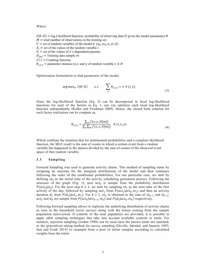
4 Results The model was trained using the Singapore Household Interview Travel Survey (HITS) 2012. Eight different activities were considered: Home, Work, Education, Eating, Shopping, Recreation, Personal, Pickup/Drop-off. Starting times and durations were discretized to an hourly basis. To validate the results, 1 million samples were generated and compared against HITS. Fig. 2 shows the results for activity transitions aggregated in the morning and the afternoon period.
(a) (b) (c)
(d) (e) (f)
Fig. 2. (a) HITS probabilities for activity transitions during the morning period (6am-12pm)
(b) Activity transitions of the 1 million samples generated during the morning period (c) Fit of the morning activity transitions of samples against HITS. SD = 0.00357
(d) HITS probabilities for activity transitions during the afternoon period (12pm-6pm) (e) Activity transitions of the 1 million samples generated during the afternoon period (f) Fit of the afternoon activity transitions of samples against HITS. SD = 0.00115
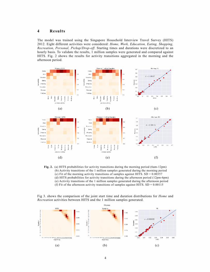
Fig 3. shows the comparison of the joint start time and duration distributions for Home and Recreation activities between HITS and the 1 million samples generated.
(a) (b) (c)
5
(d) (e) (f)
Fig. 3. (a) Joint distribution of start time and duration for Home activity in HITS
(b) Joint distribution of start time and duration for Home activity in samples (c) Fit of start time and duration joint distribution for Home. SD = 0.00103
(d) Joint distribution of start time and duration for Recreation activity in HITS (e) Joint distribution of start time and duration for Recreation activity in samples
(f) Fit of start time and duration joint distribution for Recreation. SD = 0.00045
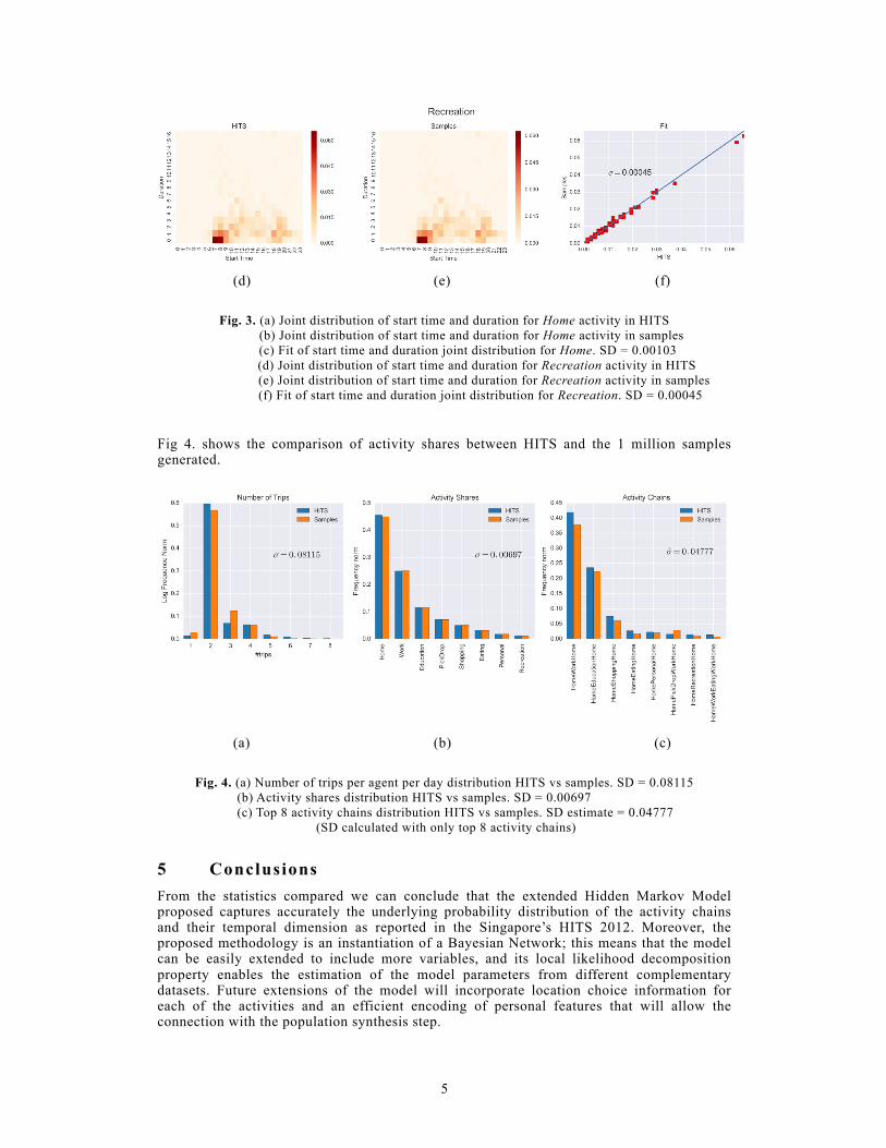
Fig 4. shows the comparison of activity shares between HITS and the 1 million samples generated.
(a) (b) (c)
Fig. 4. (a) Number of trips per agent per day distribution HITS vs samples. SD = 0.08115
(b) Activity shares distribution HITS vs samples. SD = 0.00697 (c) Top 8 activity chains distribution HITS vs samples. SD estimate = 0.04777
(SD calculated with only top 8 activity chains)
5 Conclusions From the statistics compared we can conclude that the extended Hidden Markov Model proposed captures accurately the underlying probability distribution of the activity chains and their temporal dimension as reported in the Singapore’s HITS 2012. Moreover, the proposed methodology is an instantiation of a Bayesian Network; this means that the model can be easily extended to include more variables, and its local likelihood decomposition property enables the estimation of the model parameters from different complementary datasets. Future extensions of the model will incorporate location choice information for each of the activities and an efficient encoding of personal features that will allow the connection with the population synthesis step.
6
A c k n o w l e d g m e n t s
This research has been conducted at the Singapore-ETH Centre for Global Environmental Sustainability (SEC), co-funded by the Singapore National Research Foundation (NRF) and ETH Zurich.
R e f e re n c e s Arentze, Theo A, and Harry J P Timmermans. 2004. “A Learning-Based Transportation Oriented Simulation
System.” Transportation Research Part B: Methodological 38 (7): 613–33. doi:10.1016/j.trb.2002.10.001.
Bengio, Yoshua, and Paolo Frasconi. 1995. “An Input Output HMM Architecture.” Neural Information Processing Systems, 427–34. doi:10.1093/europace/euq350.
Bhat, Chandra, Jessica Guo, Sivaramakrishnan Srinivasan, and Aruna Sivakumar. 2004. “Comprehensive Econometric Microsimulator for Daily Activity-Travel Patterns.” Transportation Research Record 1894 (1): 57–66. doi:10.3141/1894-07.
Deville, J. C., C. E. Särndal, and O Sautory. 1993. “Generalized Raking Procedures in Survey Sampling.” Journal of the American Statistical Association 88 (423): 1013–20. doi:10.1080/01621459.1993.10476369.
Jordan, Michael I. 1998. “Learning in Graphical Models.” MIT Press Cambridge Massachussets 89: 355–68. doi:10.1.1.114.4996.
Koller, Daphne, and Nir Friedman. 2009. Probabilistic Graphical Models: Principles and Techniques. Foundations. Vol. 2009. doi:10.1016/j.ccl.2010.07.006.
Miller, Eric, and Matthew Roorda. 2003. “Prototype Model of Household Activity-Travel Scheduling.” Transportation Research Record: Journal of the Transportation Research Board 1831: 114–21. doi:10.3141/1831-13.
Sun, Lijun, and Alexander Erath. 2015. “A Bayesian Network Approach for Population Synthesis.” Transportation Research Part C: Emerging Technologies 61: 49–62. doi:10.1016/j.trc.2015.10.010.
Widhalm, Peter, Bullet Yingxiang Yang, Bullet Michael Ulm, Shounak Athavale, and Bullet C Marta González. 2015. “Discovering Urban Activity Patterns in Cell Phone Data.” Transportation 42: 597–623. doi:10.1007/s11116-015-9598-x.
Yin, Mogeng, Madeleine Sheehan, Sidney Feygin, Jean-Francois Paiement, and Alexei Pozdnoukhov. 2016. “A Generative Model of Urban Activities from Cellular Data.” In ACM - KDD, 1–16. https://media.wix.com/ugd/ea3995_7ed343b025a44b0d96144622011add91.pdf.