F-16XL Hybrid Reynolds-Averaged Navier{Stokes… · F-16XL Hybrid Reynolds-Averaged...

F-16XL Hybrid Reynolds-Averaged

Navier–Stokes/Large Eddy Simulation on

Unstructured Grids

Michael A. Park,∗ Khaled S. Abdol-Hamid,† and Alaa Elmiligui‡

NASA Langley Research Center, Hampton, VA 23681

This study continues the Cranked Arrow Wing Aerodynamics Program, International(CAWAPI) investigation with the FUN3D and USM3D flow solvers. CAWAPI was estab-lished to study the F-16XL, because it provides a unique opportunity to fuse flight test,wind tunnel test, and simulation to understand the aerodynamic features of swept wings.The high-lift performance of the cranked-arrow wing planform is critical for recent and pastsupersonic transport design concepts. Simulations of the low speed high angle of attackFlight Condition 25 are compared: Detached Eddy Simulation (DES), Modified DelayedDetached Eddy Simulation (MDDES), and the Spalart-Allmaras (SA) RANS model. Iso-surfaces of Q criterion show the development of coherent primary and secondary vorticeson the upper surface of the wing that spiral, burst, and commingle. SA produces higherpressure peaks nearer to the leading-edge of the wing than flight test measurements. MeanDES and MDDES pressures better predict the flight test measurements, especially on theouter wing section. Vorticies and vortex-vortex interaction impact unsteady surface pres-sures. USM3D showed many sharp tones in volume points spectra near the wing apexwith low broadband noise and FUN3D showed more broadband noise with weaker tones.Spectra of the volume points near the outer wing leading-edge was primarily broadbandfor both codes. Without unsteady flight measurements, the flight pressure environmentcan not be used to validate the simulations containing tonal or broadband spectra. Meanforces and moment are very similar between FUN3D models and between USM3D models.Spectra of the unsteady forces and moment are broadband with a few sharp peaks forUSM3D.

I. Introduction

The Cranked-Arrow Wing Aerodynamics Project (CAWAP) was established to document upper-surfaceflow physics at high-lift and transonic test conditions and to characterize the stability and control of the F-16XL aircraft.1 Ship one, F-16XL-1, provides a unique opportunity to fuse flight test, wind tunnel test, andcomputational fluid dynamics (CFD) to understand the aerodynamic features of swept wings.2 The High-Speed Research (HSR) program identified a need to improve understanding of swept-wing aerodynamicperformance.1 High lift prediction during takeoff and landing continues to be a critical element of viablequiet supersonic aircraft concepts.3,4 Studying the high lift performance of the cranked-arrow wing planformhas been a focus for supersonic transports for decades5 and this study addresses a flow condition that isimportant for understanding pitch-up.6 Low-boom supersonic transport concepts recently developed includehighly swept7 and cranked-arrow planforms,8 which is the focus of this study.

The original CAWAP project grew into an international collaboration: the Cranked Arrow Wing Aerody-namics Program, International (CAWAPI).1 An assessment at the competition of CAWAPI9 indicated that“Overall, it can be said that the technology readiness of computational fluid dynamics simulation technologyfor the study of vehicle performance has matured since 2001, such that it can be used today with a reason-able level of confidence for complex configurations.” However, simulations at two Flight Conditions (FC),

∗Research Scientist, Computational AeroSciences Branch, AIAA Senior Member.†Research Aerospace Engineer, Configuration Aerodynamics Branch, AIAA Associate Fellow.‡Research Aerospace Engineer, Configuration Aerodynamics Branch, AIAA Senior Member.

1 of 37

American Institute of Aeronautics and Astronautics

numbered 25 and 70, did not compare as well to flight measurements as the other FCs near the center of theMach/angle of attack flight envelope. FC 25 is low speed and high angle of attack and exhibits unsteadyvortex burst phenomenon. FC 70 is a high speed case dominated by vortex-shock interaction. With theexception of two papers,10,11 analysis was performed with steady Reynolds-averaged Navier–Stokes (RANS)and Euler methods for CAWAPI.

A subsequent program12 (CAWAPI-2) targeted additional FCs near FC 25 and FC 70. These nearbyconditions were chosen primarily to help establish trends in the measured pressures associated with the vor-tex and shock structures near FC 25 and 70.12 Sensitivities to aeroelasticity and control surface deflectionwere noted.13 Finer grids and improved physics simulation due to advanced turbulence models and unsteadyhybrid RANS/Large Eddy Simulation (HRLES) resulted in improved predictions of flight test measure-ments.13 This study continues the CAWAPI-2 investigation with two simulation tools and focuses on FC25 and HRLES methods. Continued evaluation and development of HRLES models is a recommendationof the CFD Vision 2030 Study, “The use of CFD in the aerospace design process is severely limited by theinability to accurately and reliably predict turbulent flows with significant regions of separation. . . HybridRANS-LES and wall-modeled LES offer the best prospects for overcoming this obstacle although significantmodeling issues remain to be addressed here as well.”14 The study recommendation suggests this work iscritical for the development of future aerospace design methods.

Previous CAWAPI and CAWAPI-2 investigations used USM3D (Unstructured Mesh Three-Dimensional),which is also applied in this study. Lamar and Abdol-Hamid15 compared surface pressures and boundarylayer profiles computed with three RANS models to flight test measurements. Elmiligui et al.16 applied gridadaptation to these same three RANS models. Elmiligui, Abdol-Hamid, and Parlette17 applied unsteadyRANS and HRLES. This study expands the HRLES study to include FUN3D (Fully Unstructured Navier-Stokes Three-Dimensional) and examine the fluctuating pressure frequency spectra to better understand theapplication of HRLES to a cranked-arrow wing planform.

II. Flight Condition 25 and Instrumentation

This report focuses solely on FC 25, a subsonic high angle-of-attack case. The freestream flow conditionsare Mach M = 0.242, 19.84 angle of attack, and 32.22 × 106 Reynolds number based on the referencechord length. The freestream conditions are the U.S. Standard Atmosphere18 at 10,000 ft. pressure altitude.Propulsion boundary conditions are obtained from Obara and Lamar.1 FUN3D19,20 and USM3D21 nondi-mensionalize the propulsion boundary conditions with freestream conditions to produce the ratios listed inTable 1.

Table 1. Propulsion measurements and boundary conditions.

Inlet static temperature 470.1 RInlet Mach number 0.447Inlet static pressure 8.72 psia Inlet static pressure ratio 0.86265Exit total pressure 26.3 psia Exit total pressure ratio 2.6018Exit total temperature 1209 R Exit total temperature ratio 2.5029

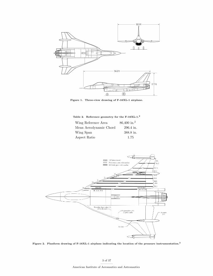
A three-view drawing of F-16XL-1 is shown in Fig. 1. The cranked-arrow planform (more sweep on theinner wing than the outer wing) is clearly evident. The geometry of the configuration is summarized inTable 2. Dummy wing tip missiles and rails are attached to each wing tip. There is an actuator pod andair dam located at the wing trailing-edge break, which is slightly inboard of the wing leading-edge break.Details of the F-16XL-1 instrumentation is available in Lamar et al.2 and the pressure measurement locationsare shown in Fig. 2. The heavy black lines denote the location of pressure belts of 0.028 in. inner diametertubing used to measure surface pressure. These pressure belts are placed at constant butt lines (BL) andhave orifices at common fuselage stations (FS), which allows comparison to simulation in either plane. Nomeasurement uncertainties or unsteady pressure measurements are available from the flight tests.

2 of 37


54.2 ft

17.7 ft

32.5 ft

Figure 1. Three-view drawing of F-16XL-1 airplane.

Table 2. Reference geometry for the F-16XL-1.2

Wing Reference Area 86,400 in.2

Mean Aerodynamic Chord 296.4 in.Wing Span 388.8 in.Aspect Ratio 1.75

Figure 2. Planform drawing of F-16XL-1 airplane indicating the location of the pressure instrumentation.2

3 of 37


III. Numerical Approach

The focus of this report is applying the HRLES capabilities of FUN3D and USM3D. First, these flowsolvers and the HRLES methods are described. Then details on the time step and grids are provided.

III.A. FUN3D

FUN3D20 is a node-centered finite volume scheme (the solution is stored at grid nodes). Anderson andBonhaus22 describe the reconstruction scheme for inviscid terms, the viscous discretization, and solutionscheme, which results in a nominally second-order spatial discretization. The Roe23 approximate Riemannsolver is used in this study. The Optimized Second Order Backward Difference (BDF2OPT)24 is used for timeadvancement of the unsteady simulations. Steady results are computed with the Spalart-Allmaras25 (SA)turbulence model. Both DES26 (Detached Eddy Simulation) and MDDES27 (Modified DDES28 (DelayedDES)) are used for the unsteady results. MDDES was developed to alleviate pockets of large eddy viscosity inregions upstream of a cylinder in testing.27 The MDDES simulations use SA-R29,30 and the DES simulationsuse SA for the RANS portion of HRLES. The advantage of using SA-R with MDDES is that the eddy viscosityis reduced in the regions that have higher vorticity than strain rate, such as in the vortex core where thepure rotation should suppress the turbulence.29 These HRLES capabilities in FUN3D have been comparedto wind tunnel and flight measurement for aeroacoustics,27,31 unsteady launch vehicle aerodynamics,32 andF-15 vertical tail buffet.33

III.B. USM3D

USM3D34 is a cell-centered finite volume flow solver (the solution is stored at tetrahedra centers). Thespatial discretization in nominally second-order and it is part of TetrUSS (Tetrahedral Unstructured SoftwareSystem).35 USM3D uses advanced turbulence models36 and second-order temporal schemes for unsteadyflows.37 Three-point backward differencing and pseudo-time subiterations are used for time integration,which is referred to as Option-1 in Elmiligui, Abdol-Hamid, and Parlette.17 Frink38 describes the inviscidinterface reconstruction scheme used with the Roe23 flux and the viscous discretization. Forces, moments,and spectra of unsteady pressure for DES cases examined in Elmiligui, Abdol-Hamid, and Parlette17 aredetailed in this report. The mean values of surface pressures at BL and FS are provided by Elmiligui,Abdol-Hamid, and Parlette,17 but not reproduced in this report. In this study, USM3D results use the DESHRLES model and are explicitly labeled with the flow solver name.

III.C. Temporal Integration

FUN3D uses the BDF2OPT24,39 time advancement scheme for the HRLES cases. USM3D uses the three-point backward differencing and pseudo-time subiteration scheme described by Elmiligui et al.17 as Option-1.The surface pressures computed with Option-1 showed a small sensitivity to time step.17 Both FUN3D20

and USM3D37 nondimensionalize time with the freestream speed of sound and the grid unit length. A timestep ∆t is typically chosen by selecting a fraction (1/N) of the nondimensional time required for a particleto travel at freestream Mach number M a characteristic distance L,

∆t =L

MN, (1)

where L is the mean aerodynamic chord. All the unsteady FUN3D results used ∆t = 1.2248 = 296.4/(0.242×1000). The USM3D results used ∆t = 5 and ∆t = 1. The FUN3D physical time step is ∆t = 9.4747× 10−5

seconds assuming a freestream speed of sound of 12, 927 in. per second (1,077.2 ft. per second) at standard-day 10,000 ft. pressure altitude. The two USM3D physical time steps are ∆t = 7.7358 × 10−5 and ∆t =3.8679 × 10−4 seconds. The FUN3D averaging windows are 8,000 time steps, which is approximately 0.76seconds or eight free stream passages of the mean aerodynamic chord. USM3D used 16,000 time steps or1.24 seconds for the fine time step size and 6,000 time steps or 2.32 seconds for the coarse time step size.These data are extracted after the initial start up transients have decayed.

III.D. Grids

Details of the half domain grids used in this study (including images of the surface grid and volume slices)are provided by Elmiligui et al.16 and are summarized in Table 3. The sides of the outer domain box are

4 of 37


approximately 50 mean aerodynamic chords in length. Elmiligui et al.17 provides further details of thehalf domain grids (denoted Grid-1) and shows that mirroring the grids to include both starboard and porthalves of the aircraft (denoted Grid-2) had a negligible effect on the averaged HRLES surface pressures.As a result of this observation, only the half domain grids will be used for the zero sideslip cases in thisarticle. FUN3D stores the flow solution at the nodes of the mesh and USM3D stores the the flow solutionat the tetrahedra centers. Therefore, nodes indicates the resolution of the FUN3D solutions and tetrahedraindicates the resolution USM3D solutions. The USM3D results labeled with 19M indicate the number oftetrahedra in the coarse grid. The FUN3D results are labeled with 11M and 24M to indicate the numberof nodes in the medium and fine grids. The given first cell heights result in an average y+ = 1.1 for thecoarse grid and less on the finer meshes.16,17 The grids were constructed with guidelines from the AIAADrag Prediction and High Lift Prediction Workshops16 and no additional refinement was added to resolveoff-body vorticies or turbulent structures. The grid is in full-scale inches, which corresponds to the units ofBL, FS, and water line (WL).

Table 3. Grids.

Description Nodes Tetrahedra First cell height (in.)Coarse 3,302,181 19,369,037 0.00092Medium 10,635,136 62,472,142 0.00061Fine 24,330,073 143,034,292 0.00041

IV. Results

Isosurfaces colored with pressure coefficient are provided to show a global view of the upper wind flowfeatures and qualitative differences between a RANS and the two HRLES methods. Medium and fine gridsare shown to indicate how grid refinement helps to resolve the features. Next, mean pressure coefficient isshown at constant BL and FS. This is a typical comparison that is made to flight test measurements inCAWAPI reports.

Unsteady results begin with surface plots of standard deviation of fluctuating surface pressure coefficient.This provides a global view of the relative magnitude of unsteadiness on the upper fuselage, lower fuselage,engine inlet, and exhaust plume. More details are provided at FS and BL by showing one standard deviationof pressure coefficient around the mean.

Points are sampled in the volume to compute standard deviation. Frequency spectra are examined atpoints that exhibit large standard deviation magnitude and changes in magnitude between medium and finegrids. Statistics and frequency spectra of integrated forces and moment complete the examination of theunsteady solution.

IV.A. Isosurfaces

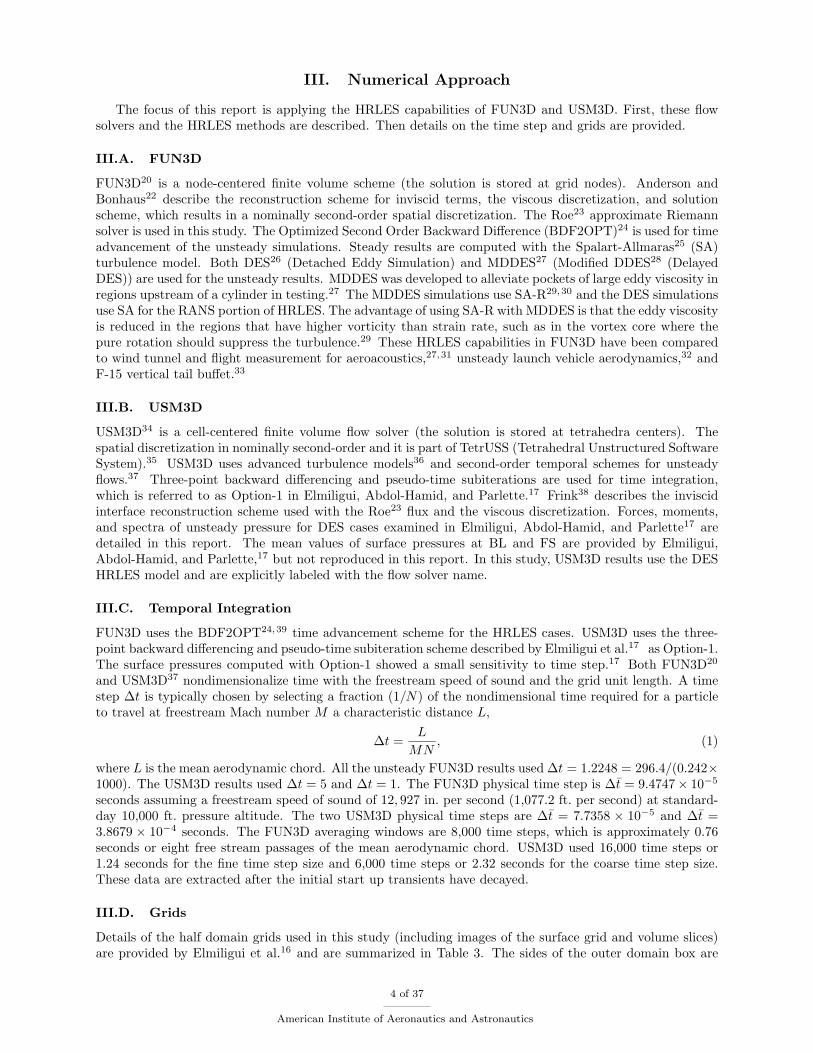
Isosurfaces of Q criterion40 are provided for FUN3D to gain a global intuition for the location of vorticespredicted by each turbulence model. Q criterion is defined as,

Q =12

(||Ω||2 − ||S||2

), (2)

where Ω is the rotation rate tensor, S is the strain rate tensor, and || · || is the Frobenius norm. Positive Qdefines regions where the vorticity magnitude is greater than the strain-rate magnitude. Snapshots, at theend of the simulation, are shown for the Q = 0.001 isosurface colored with pressure coefficient in Fig. 3 toFig. 7. The wing upper surface is shown for four models. Only one half of the domain is simulated withthe surfaces mirrored in the x–z plane to provide two views of the vortical structures and depict the entiresymmetric domain. The steady-state solution with SA is shown for two grid resolutions in Fig. 3. Distinctsets of vortices are observed at the wing apex, air dam, outer wing, and surrounding the dummy missile.The isosurfaces of the SA solution appear to be insensitive to grid resolution for these two grid resolutions.The extent of the vorticies is the smallest for all models. The vorticity-based source term of SA predicts anexcessive level of eddy viscosity, which dissipates the vorticies.

5 of 37


Snapshots of the DES simulations are shown in Fig. 4. Vortices are maintained for a longer distance downstream as compared to SA. The main wing leading-edge vortices spiral and break into filaments. Secondaryvortices are seen below the main vortex, near the wing leading-edge. The significant difference between DESon the medium and fine grids indicates a strong dependence on grid resolution for these 11M and 24M nodegrids. On the fine grid, the secondary vortices are breaking into filaments and becoming entrained on themain vortex. Vortex breakup is evident in the outer wing and the distinct vortices seen on the medium gridcommingle.

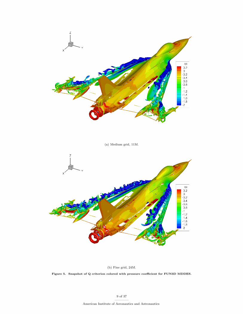
Snapshots of the MDDES simulations are shown in Fig. 5. The medium grid simulation exhibits thebreakup of the secondary vortices seen in the fine DES simulation. The topology of the medium and finegrid flow structures is similar with the fine grid exhibiting finer details. The main vortex begins to spiral verynear the wing apex. The secondary wing leading-edge vortices are clearly entrained into the main vortex.Secondary wing leading-edge vortex filaments are transported down the wing leading-edge and disrupt thecoherence of the outer wing vortex. Vortices that surround the dummy wing tip missile rail, body, and finsmix with the outer wing vortex filaments.

Views of the top and starboard side are shown for the half of the aircraft simulated with the HRLESmethods DES (Fig. 6) and MDDES (Fig. 7). The coherent secondary wing leading-edge vortex of the mediumgrid is seen in Fig. 6(b), which breaks up on the fine grid, Fig. 6(c and d). The entrainment of the secondaryvortex around the main vortex is seen in Fig. 7(c) and the commingling of the vortex filaments is seen inFig. 7(d). The pressure footprint of the vortex filaments can also be seen in Fig. 7(d) snapshot with pressuresalternating above and below freestream pressure on the outer wing section.

6 of 37


(a) Medium grid, 11M.

(b) Fine grid, 24M.

Figure 3. Snapshot of Q criterion colored with pressure coefficient for FUN3D SA.

7 of 37



(b) Fine grid, 24M.

Figure 4. Snapshot of Q criterion colored with pressure coefficient for FUN3D DES.

8 of 37



(b) Fine grid, 24M.

Figure 5. Snapshot of Q criterion colored with pressure coefficient for FUN3D MDDES.

9 of 37


(a) Medium grid, 11M, side view.

(b) Medium grid, 11M, top-down view.

(c) Fine grid, 24M, side view.

(d) Fine grid, 24M, top-down view.

Figure 6. Snapshot of Q criterion colored with pressure coefficient for FUN3D DES.

10 of 37


(a) Medium grid, 11M, side view.

(b) Medium grid, 11M, top-down view.

(c) Fine grid, 24M, side view.

(d) Fine grid, 24M, top-down view.

Figure 7. Snapshot of Q criterion colored with pressure coefficient for FUN3D MDDES.

11 of 37


IV.B. Mean Section Cut Pressures

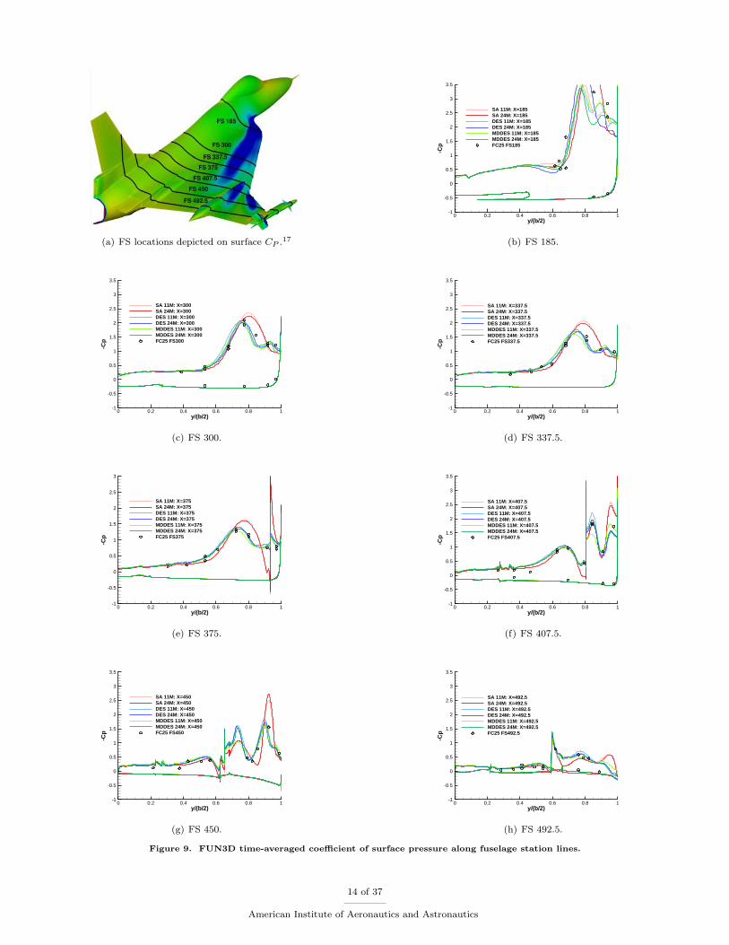
The mean surface pressure coefficient is shown for constant BL slices in Fig. 8 and constant FS slices in Fig. 9.The negative pressure coefficient is depicted; a positive value is suction. The x position is nondimensionalizedwith local chord and the y position with local wing span, which excludes the dummy missile and rail. Thedummy missile and rail are excluded from this presentation because their location is y/(b/2) > 1. The peakvalues of BL 55 and FS 185 negative pressure coefficient are clipped to use the same −CP scale as companionCAWAPI papers. The BL 55 SA 24M has a peak of −CP = 3.75 at x/c = 0.045, the FS 185 DES 24M has apeak of −CP = 4.30 at y/(b/2) = 0.79, and the FS 185 SA 24M has a peak of −CP = 4.45 at y/(b/2) = 0.84.The heights of these clipped peaks are higher than the values reported by other CAWAPI participants andthe flight test measurements.

Overall, SA on both grids overpredicts the suction peaks and displaces these peaks forward or outboard(nearer to the wing leading-edge). Elmiligui, Abdol-Hamid, and Parlette17 show in their Fig. 9 that the peakof USM3D SA results are also more forward and outboard of the DES mean pressure and flight measurements,but these peaks are lower for the 62M tetrahedra medium grid than the FUN3D SA results. The HRLESmethods are closer to the flight test measurements (circles) than SA for a majority of the measurements.The most variation between methods is seen in the wing apex region, the forward portion of BL 55 and BL70.

The air dam is seen in FS 375 and greater as a vertical line in the simulations. This air dam, describedas a wing fence by Grafton,41 was added to improve lateral and pitch stability at high angles of attack, butis detrimental to vortex lift. This report shows that more suction is maintained on the outer wing uppersurface outboard of the air dam, which has a favorable impact on pitch-up and lateral stability. Two meansuction peaks are seen in FS 407.5 and FS 450 outboard of the air dam, which are due to the air dam vortexand outer wing leading-edge vortex. SA has very different −CP levels in the outer section of the wing, BL184.5, where MDDES 11M has a slightly higher mean than the other HRLES methods.

12 of 37


(a) BL locations depicted on surface CP .17

x/c

-Cp

0 0.2 0.4 0.6 0.8 1-1

-0.5

0

0.5

1

1.5

2

2.5

3

3.5

SA 11M: Y=55SA 24M: Y=55DES 11M: Y=55DES 24M: Y=55MDDES 11M: Y=55MDDES 24M: Y=55FC25 BL55

(b) BL 55.

x/c

-Cp

0 0.2 0.4 0.6 0.8 1-1

-0.5

0

0.5

1

1.5

2

2.5

3

3.5


(c) BL 70.

x/c

-Cp

0 0.2 0.4 0.6 0.8 1-1

-0.5

0

0.5

1

1.5

2

2.5

3

3.5


(d) BL 80.

x/c

-Cp

0 0.2 0.4 0.6 0.8 1-1

-0.5

0

0.5

1

1.5

2

2.5

3

3.5


(e) BL 95.

x/c

-Cp

0 0.2 0.4 0.6 0.8 1-1

-0.5

0

0.5

1

1.5

2

2.5

3

3.5


(f) BL 105.

x/c

-Cp

0 0.2 0.4 0.6 0.8 1-1

-0.5

0

0.5

1

1.5

2

2.5

3

3.5

SA 11M: Y=153.5SA 24M: Y=153.5DES 11M: Y=153.5DES 24M: Y=153.5MDDES 11M: Y=153.5MDDES 24M: Y=153.5FC25 BL153.5

(g) BL 153.5.

x/c

-Cp

0 0.2 0.4 0.6 0.8 1-1

-0.5

0

0.5

1

1.5

2

2.5

3

3.5

SA 11M: Y=184.5SA 24M: Y=184.5DES 11M: Y=184.5DES 24M: Y=184.5MDDES 11M: Y=184.5MDDES 24M: Y=184.5FC25 BL184.5

(h) BL 184.5.

Figure 8. FUN3D time-averaged coefficient of surface pressure along butt lines.

13 of 37


(a) FS locations depicted on surface CP .17

y/(b/2)

-Cp

0 0.2 0.4 0.6 0.8 1-1

-0.5

0

0.5

1

1.5

2

2.5

3

3.5

SA 11M: X=185SA 24M: X=185DES 11M: X=185DES 24M: X=185MDDES 11M: X=185MDDES 24M: X=185FC25 FS185

(b) FS 185.

y/(b/2)

-Cp

0 0.2 0.4 0.6 0.8 1-1

-0.5

0

0.5

1

1.5

2

2.5

3

3.5


(c) FS 300.

y/(b/2)

-Cp

0 0.2 0.4 0.6 0.8 1-1

-0.5

0

0.5

1

1.5

2

2.5

3

3.5

SA 11M: X=337.5SA 24M: X=337.5DES 11M: X=337.5DES 24M: X=337.5MDDES 11M: X=337.5MDDES 24M: X=337.5FC25 FS337.5

(d) FS 337.5.

y/(b/2)

-Cp

0 0.2 0.4 0.6 0.8 1-1

-0.5

0

0.5

1

1.5

2

2.5

3


(e) FS 375.

y/(b/2)

-Cp

0 0.2 0.4 0.6 0.8 1-1

-0.5

0

0.5

1

1.5

2

2.5

3

3.5


(f) FS 407.5.

y/(b/2)

-Cp

0 0.2 0.4 0.6 0.8 1-1

-0.5

0

0.5

1

1.5

2

2.5

3

3.5


(g) FS 450.

y/(b/2)

-Cp

0 0.2 0.4 0.6 0.8 1-1

-0.5

0

0.5

1

1.5

2

2.5

3

3.5


(h) FS 492.5.

Figure 9. FUN3D time-averaged coefficient of surface pressure along fuselage station lines.

14 of 37


IV.C. Surface Pressure Fluctuations

Unfortunately, there were no unsteady flow measurements made during the flight tests, but unsteady pres-sures are examined here to illustrate the differences in the HRLES methods and the effect of increasinggrid resolution. These results also provide a database for code-to-code comparison with other CAWAPIparticipants. To gain a global picture of the unsteady pressure loads on the vehicle, the standard deviationof pressure coefficient is studied for the HRLES methods. This standard deviation is also referred to as theroot mean square (RMS) of the pressure coefficient variation from the mean.

RMS pressure coefficient on the upper surface and symmetry plane is shown for DES in Fig. 10 with alogarithmic color scale. The footprint of the unsteady vorticies are seen at the apex, air dam, and outer wingsection. A high level of unsteadiness is also seen in the engine exhaust plume diamond shock pattern. TheRMS levels are higher for the fine grid. RMS pressure coefficient on the lower surface and symmetry planeis shown for DES in Fig. 11. The engine inlet, wing leading-edge, wing trailing-edge, and engine exhaustplume have the highest levels of unsteadiness. The medium grid has an unexplained patch of unsteadinessin front of the wing, below the leading-edge of the canopy. There is no vortex indicated in Fig. 6(a) nearthis patch, which is not seen on the fine grid.

RMS pressure coefficient on the upper surface and symmetry plane is shown for MDDES in Fig. 12. Thestructures are the same as DES, but the levels are higher. The medium grid (Fig. 12(a)) has a lower levelof RMS pressure at the wing apex than the fine grid (Fig. 12(b)), but the medium grid has a higher level ofunsteadiness on the outer wing section. This MDDES case on the medium 11M node grid also has slightlydifferent mean values at outer wing section as seen in Fig. 8(f and g) and Fig. 9(e, f, and g). The mediumgrid MDDES has the same unexplained patch of unsteadiness in front of the wing as seen on the mediumgrid DES.

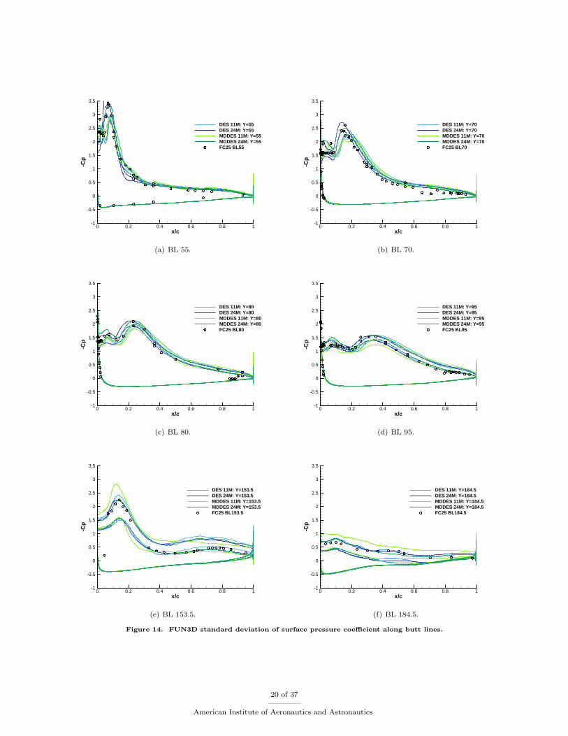
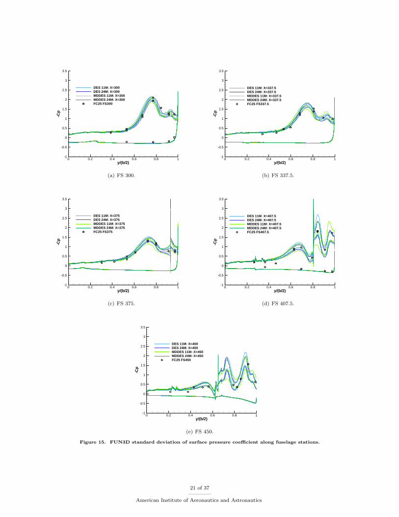
One standard deviation of unsteady pressures is shown above and below the mean for constant BL andFS stations in Fig. 14 and Fig. 15. The BL 55 DES 24M mean plus RMS peak of −CP = 3.76 at x/c = 0.05was clipped to have a consistent range with companion CAWAPI report plots. The variation of lower wingsurface pressures is much lower than the upper surface pressures. The lowest level of variation on the uppersurface is inboard, particularly over the fuselage. The variation range of methods on both grid is similarfor the inner wing, but the MDDES 11M medium grid has a slightly higher range on the outer wing, seeFig. 14(e and f) and Fig. 15(d and e). Most of the the flight test measurements are within the unsteadyvariation of the HRLES methods on both grids. The flight measurements are assumed to be time-averagedmean data, but the unsteady flight pressure may be filtered by the long lengths of 0.028 in. inner diametertubing used for instrumentation.2

15 of 37



(b) Fine grid, 24M.

Figure 10. Upper surface pressure coefficient RMS variation for FUN3D DES.

16 of 37



(b) Fine grid, 24M.

Figure 11. Lower surface pressure coefficient RMS variation for FUN3D DES.

17 of 37



(b) Fine grid, 24M.

Figure 12. Upper surface pressure coefficient RMS variation for FUN3D MDDES.

18 of 37



(b) Fine grid, 24M.

Figure 13. Lower surface pressure coefficient RMS variation for FUN3D MDDES.

19 of 37


x/c

-Cp

0 0.2 0.4 0.6 0.8 1-1

-0.5

0

0.5

1

1.5

2

2.5

3

3.5

DES 11M: Y=55DES 24M: Y=55MDDES 11M: Y=55MDDES 24M: Y=55FC25 BL55

(a) BL 55.

x/c

-Cp

0 0.2 0.4 0.6 0.8 1-1

-0.5

0

0.5

1

1.5

2

2.5

3

3.5


(b) BL 70.

x/c

-Cp

0 0.2 0.4 0.6 0.8 1-1

-0.5

0

0.5

1

1.5

2

2.5

3

3.5


(c) BL 80.

x/c

-Cp

0 0.2 0.4 0.6 0.8 1-1

-0.5

0

0.5

1

1.5

2

2.5

3

3.5


(d) BL 95.

x/c

-Cp

0 0.2 0.4 0.6 0.8 1-1

-0.5

0

0.5

1

1.5

2

2.5

3

3.5

DES 11M: Y=153.5DES 24M: Y=153.5MDDES 11M: Y=153.5MDDES 24M: Y=153.5FC25 BL153.5

(e) BL 153.5.

x/c

-Cp

0 0.2 0.4 0.6 0.8 1-1

-0.5

0

0.5

1

1.5

2

2.5

3

3.5

DES 11M: Y=184.5DES 24M: Y=184.5MDDES 11M: Y=184.5MDDES 24M: Y=184.5FC25 BL184.5

(f) BL 184.5.

Figure 14. FUN3D standard deviation of surface pressure coefficient along butt lines.

20 of 37


y/(b/2)

-Cp

0 0.2 0.4 0.6 0.8 1-1

-0.5

0

0.5

1

1.5

2

2.5

3

3.5

DES 11M: X=300DES 24M: X=300MDDES 11M: X=300MDDES 24M: X=300FC25 FS300

(a) FS 300.

y/(b/2)

-Cp

0 0.2 0.4 0.6 0.8 1-1

-0.5

0

0.5

1

1.5

2

2.5

3

3.5

DES 11M: X=337.5DES 24M: X=337.5MDDES 11M: X=337.5MDDES 24M: X=337.5FC25 FS337.5

(b) FS 337.5.

y/(b/2)

-Cp

0 0.2 0.4 0.6 0.8 1-1

-0.5

0

0.5

1

1.5

2

2.5

3

3.5


(c) FS 375.

y/(b/2)

-Cp

0 0.2 0.4 0.6 0.8 1-1

-0.5

0

0.5

1

1.5

2

2.5

3

3.5

DES 11M: X=407.5DES 24M: X=407.5MDDES 11M: X=407.5MDDES 24M: X=407.5FC25 FS407.5

(d) FS 407.5.

y/(b/2)

-Cp

0 0.2 0.4 0.6 0.8 1-1

-0.5

0

0.5

1

1.5

2

2.5

3

3.5


(e) FS 450.

Figure 15. FUN3D standard deviation of surface pressure coefficient along fuselage stations.

21 of 37


IV.D. Volume Point Pressure Fluctuations

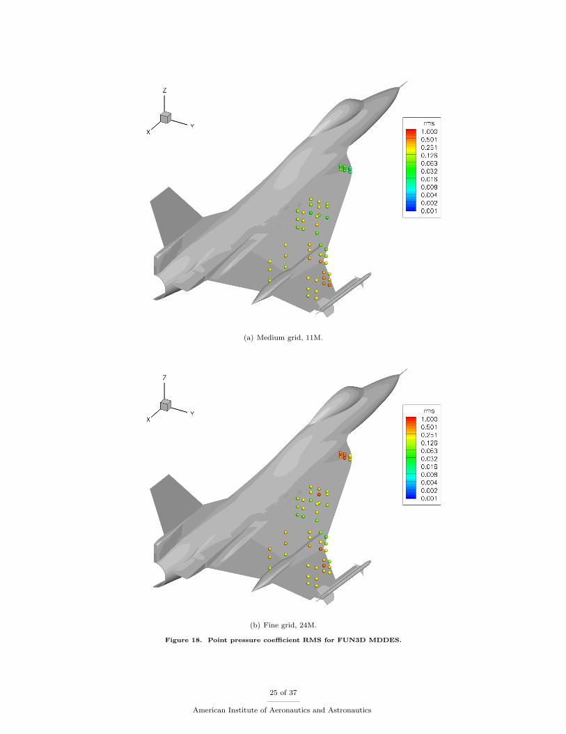
Pressure coefficient is sampled at a number of points in the domain to examine the off-body flow unsteadiness.These points are arranged in groups of three that extend in the WL direction at constant BL and FS. RMSof pressure coefficient is shown for USM3D DES on the coarse 19M tetrahedra grid in Fig. 16 for two timestep sizes. The level of unsteadiness appears uniform for this logarithmic color scale of RMS. The FUN3DDES results in Fig. 17 show a higher RMS level than USM3D, particularly on the outer wing section andfine grid apex. The FUN3D MDDES results in Fig. 18 show similar RMS levels as the DES results.

Spectra are computed via the method of Welch42 as implemented in the Octave-Forge pwelsh function.43

Segments of 211 = 2048 points are used with 50% overlap between segments with the mean subtracted andthe application of a Hamming window. The spectra for two groups of point samples denoted “Apex” and“Outer Wing Leading-Edge” in Fig. 19 are detailed. Sound pressure level (SPL) is computed with a referencesound pressure of 20µPa. These groups are selected because they have a high RMS level on the fine grid andthere is significant variation in the levels between methods and grid resolutions. Frequencies are reported infull-scale, see Section III.C for simulation time step information and Section III.D for grid descriptions. Theapex spectra are examined first.

The USM3D apex spectra are shown in Fig. 20. A series of strong tones are depicted. The three largestpeak tones are 116 Hz, 233 Hz, and 350 Hz for ∆t = 5 and 130 Hz, 260 Hz, 389 Hz for ∆t = 1. The FUN3DDES is primarily broadband noise with a weak tone at 164 Hz for the medium grid and 130 Hz for the finegrid, Fig. 21. MDDES shows a significant peak at 144 Hz for the medium grid at 165 Hz and 371 Hz forthe fine grid, Fig. 22. There does not appear to be a single tone that is predicted consistently by thesecombinations of methods and grids. DES and MDDES on the fine grid show very similar broadband noisespectra.

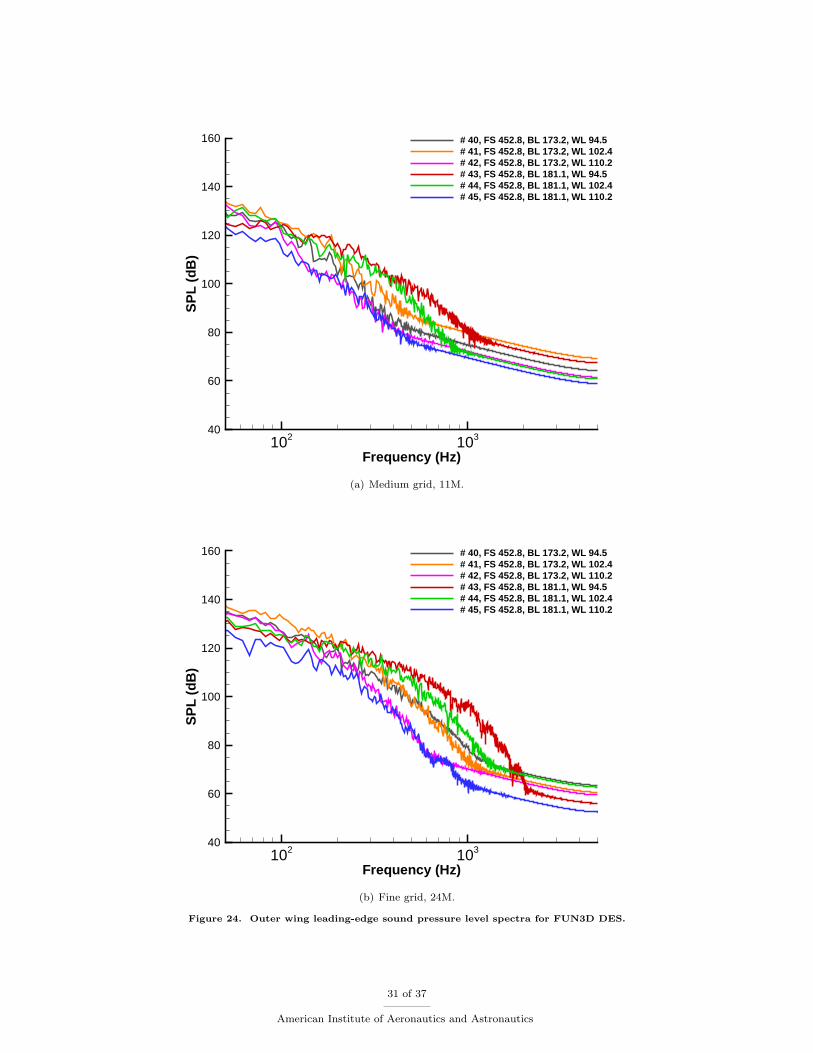
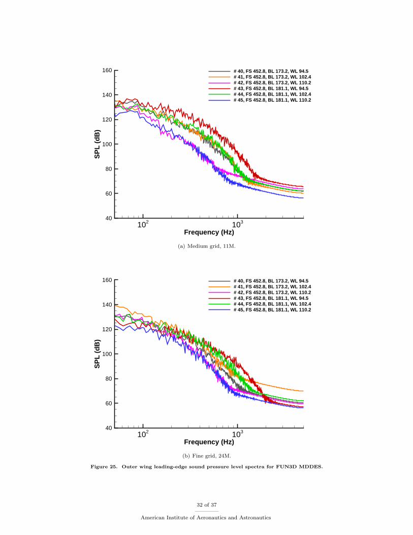
The USM3D outer wing leading-edge spectra are shown in Fig. 23. The ∆t = 5 simulation exhibits onetone at 76 Hz and a steep roll-off at 200 Hz. The FUN3D DES (Fig. 24) and FUN3D MDDES (Fig. 25)signals are broadband for the outer wing leading-edge spectra. MDDES 11M has the most energy between100 and 1,000 Hz of all the methods. Both USM3D DES time steps and FUN3D DES 11M spectra dropbelow 80 dB at 1,000 Hz, but the other FUN3D results have energy above 80 dB at 1,000 Hz.

Without unsteady flight measurements, the flight pressure environment can not be used to determinewhether broadband spectra or tonal spectra predictions are appropriate for these locations. A lack ofconsistent tone frequency predictions may indicate that the tones are an artifact of the simulation or thatthe flow features have not been sufficiently resolved in space or time.

22 of 37


(a) Large time step, ∆t = 5.

(b) Small time step, ∆t = 1.

Figure 16. Point pressure coefficient RMS for USM3D DES, coarse grid, 19M.

23 of 37



(b) Fine grid, 24M.

Figure 17. Point pressure coefficient RMS for FUN3D DES.

24 of 37



(b) Fine grid, 24M.

Figure 18. Point pressure coefficient RMS for FUN3D MDDES.

25 of 37


(a) Apex point group.

(b) Outer wing leading-edge point group.

Figure 19. Point pressure coefficient RMS groups.

26 of 37


Frequency (Hz)

SP

L (

dB

)

102 10340

60

80

100

120

140

160

# 1, FS 196.9, BL 49.2, WL 94.5# 2, FS 196.9, BL 49.2, WL 98.4# 3, FS 196.9, BL 49.2, WL 100.4# 4, FS 196.9, BL 55.1, WL 94.5# 5, FS 196.9, BL 55.1, WL 98.4# 6, FS 196.9, BL 55.1, WL 100.4# 7, FS 196.9, BL 63.0, WL 94.5# 8, FS 196.9, BL 63.0, WL 98.4# 9, FS 196.9, BL 63.0, WL 100.4


Frequency (Hz)

SP

L (

dB

)

102 10340

60

80

100

120

140

160



Figure 20. Apex sound pressure level spectra for USM3D DES, coarse grid, 19M.

27 of 37


Frequency (Hz)

SP

L (

dB

)

102 10340

60

80

100

120

140

160



Frequency (Hz)

SP

L (

dB

)

102 10340

60

80

100

120

140

160


(b) Fine grid, 24M.

Figure 21. Apex sound pressure level spectra for FUN3D DES.

28 of 37


Frequency (Hz)

SP

L (

dB

)

102 10340

60

80

100

120

140

160



Frequency (Hz)

SP

L (

dB

)

102 10340

60

80

100

120

140

160


(b) Fine grid, 24M.

Figure 22. Apex sound pressure level spectra for FUN3D MDDES.

29 of 37


Frequency (Hz)

SP

L (

dB

)

102 10340

60

80

100

120

140

160 # 40, FS 452.8, BL 173.2, WL 94.5# 41, FS 452.8, BL 173.2, WL 102.4# 42, FS 452.8, BL 173.2, WL 110.2# 43, FS 452.8, BL 181.1, WL 94.5# 44, FS 452.8, BL 181.1, WL 102.4# 45, FS 452.8, BL 181.1, WL 110.2


Frequency (Hz)

SP

L (

dB

)

102 10340

60

80

100

120

140



Figure 23. Outer wing leading-edge sound pressure level spectra for USM3D DES, coarse grid, 19M.

30 of 37


Frequency (Hz)

SP

L (

dB

)

102 10340

60

80

100

120

140



Frequency (Hz)

SP

L (

dB

)

102 10340

60

80

100

120

140


(b) Fine grid, 24M.

Figure 24. Outer wing leading-edge sound pressure level spectra for FUN3D DES.

31 of 37


Frequency (Hz)

SP

L (

dB

)

102 10340

60

80

100

120

140



Frequency (Hz)

SP

L (

dB

)

102 10340

60

80

100

120

140


(b) Fine grid, 24M.

Figure 25. Outer wing leading-edge sound pressure level spectra for FUN3D MDDES.

32 of 37


IV.E. Forces and Moment

Mean, RMS, minimum, and maximum integrated coefficient of lift CL, drag CD, and pitching moment CM

are examined for the entire sampling window in Table 4. For reference, an F-16XL wind tunnel test withflow thorough inlet, wing fence (air dam), nose boom, and missiles at Reynolds number 2.1× 106 based onmean aerodynamic chord, 20 angle of attack, and 0 angle of sideslip is provided. This test point is fromrun 200 by Hahne44 and differs from the simulation in Reynolds number and propulsion modeling. Lift isslightly higher and drag is significantly lower than the mean simulation forces. The mean forces are similarbetween the SA and HRLES FUN3D results. The USM3D DES has slightly lower lift and higher drag thanthe FUN3D results. The large time step USM3D has the lowest RMS levels. The FUN3D MDDES 11M hasthe highest RMS levels. The remaining HRLES methods are within 15% for RMS CL and CD.

Table 4. Forces and moment.

Case CmeanL Crms

L (CminL − Cmax

L ) CmeanD Crms

D (CminD − Cmax

D ) CmeanM Crms

M (CminM − Cmax

M )

WT 0.8405 0.2693 -0.0052

FUN3D SA 11M 0.8036 0.4478 0.0025

FUN3D SA 24M 0.8041 0.4507 0.0024

USM3D DES 19M ∆t = 5 0.7605 0.0037 (0.7503-0.7725) 0.4823 0.0012 (0.4791-0.4860) 0.0072 0.0022 (-0.0002-0.0124)

USM3D DES 19M ∆t = 1 0.7507 0.0055 (0.7347-0.7656) 0.4801 0.0018 (0.4753-0.4845) 0.0062 0.0034 (-0.0025-0.0163)

FUN3D DES 11M 0.8015 0.0054 (0.7880-0.8138) 0.4513 0.0017 (0.4462-0.4555) -0.0057 0.0030 (-0.0145-0.0013)

FUN3D DES 24M 0.8021 0.0058 (0.7868-0.8180) 0.4526 0.0020 (0.4476-0.4577) -0.0037 0.0026 (-0.0115-0.0022)

FUN3D MDDES 11M 0.7939 0.0088 (0.7688-0.8159) 0.4463 0.0030 (0.4375-0.4528) -0.0021 0.0041 (-0.0121-0.0090)

FUN3D MDDES 24M 0.8020 0.0054 (0.7870-0.8180) 0.4528 0.0020 (0.4472-0.4585) -0.0021 0.0025 (-0.0108-0.0044)

The same method is used to compute the spectra of integrated forces and moments as the volumepressures. Spectra are computed via the method of Welch42 as implemented in the Octave-Forge pwelshfunction.43 Segments of 211 = 2048 points are used with 50% overlap between segments with the meansubtracted and the application of a Hamming window. USM3D has the lowest broadband noise levels withpeaks at 76 Hz, 116 Hz, and 232 Hz for ∆t = 5 and 130 Hz ∆t = 1. The peaks of force and moment spectraat 116 Hz and 232 Hz at the same frequencies the 116 Hz and 233 Hz observed in the ∆t = 5 volume apexpoint spectra. The unsteady forces are broadband for FUN3D with the levels increasing with grid refinementand from DES to MDDES.

33 of 37


Frequency (Hz)

CL2 /H

z

101 102 10310-15

10-13

10-11

10-9

10-7

10-5

USM3D 19M dt=5USM3D 19M dt=1FUN3D DES 11MFUN3D DES 24MFUN3D MDDES 11MFUN3D MDDES 24M

(a) Lift coefficient.

Frequency (Hz)

CD2 /H

z

101 102 10310-15

10-13

10-11

10-9

10-7

10-5


(b) Drag coefficient.

Frequency (Hz)

CM2 /H

z

101 102 10310-15

10-13

10-11

10-9

10-7

10-5


(c) Pitching moment coefficient.

Figure 26. Power spectral density of forces.

34 of 37


V. Conclusions

The HRLES model in FUN3D and USM3D are applied to the F-16XL-1 in the framework of the CAWAPIproject. Q criteria isosurfaces provide a global view of the vortex structures, their coherency, and how thesevortices interact. Mean surface pressure coefficient at constant BL and FS indicated that steady RANS SAoverpredicted the maximum value of suction peak and predicted it too near the wing leading-edge. MeanHRLES pressures provide a better comparison to flight test measurements. The mean pressure coefficienthas the most spread between methods in the wing apex region. The outer wing has clear indication of theaverage suction peaks of both air dam and wing leading-edge vortices. The medium 11M node MDDESsolution has a different mean value than the other HRLES models for outer wing upper surface. Both SAresolutions have a stronger wing leading-edge vortex suction and weaker air dam vortex suction than theHRLES mean pressure.

RMS values of unsteady surface pressure coefficients provide a global view of the unsteadiness and therelative magnitude of the variation over the entire aircraft. The medium grid HRLES simulations have aquieter wing apex and higher levels of unsteadiness in the outer wing section than fine grid HRLES. Themedium grid HRLES simulations have a patch of unsteadiness on the side of the forward fuselage not seenon the fine grid or the Q criteria isosurface.

USM3D had lower levels of RMS pressure at sampled volume points. The fine grid FUN3D HRLES hashigher RMS values for the apex than medium grid HRLES or USM3D. Many of the volume points over theouter portion of the wing exhibited high RMS values, particularly at the wing leading-edge and near theair dam. These high levels are most likely due to vorticies in those regions that can be seen to be spiralingand commingling in the Q criteria isosurfaces. USM3D apex volume points have many pure tones withlow broadband noise. FUN3D shows weak tones and a dramatic increase in apex broadband noise with gridrefinement. The outer wing leading-edge spectra has a similar broadband shape for all methods. These outerwing points are less sensitive to time step and grid refinement. The medium 11M node grid MDDES has thehighest level of outer-wing leading-edge broadband noise, which is also seen in RMS surface pressures. Themedium 11M MDDES also has a slightly different mean coefficient pressure than the other three FUN3DHRLES simulations.

The forces and moment spectra are primarily broadband. The exceptions are the tones seen in the largetime step USM3D apex volume points are present in the forces and moments for that model. The meanvalues of lift and drag of the FUN3D models are very similar. The mean USM3D lift, drag, and pitchingmoment are similar for the two different time step sizes, but lower in lift, higher in drag, and higher inpitching moment than the FUN3D means.

As seen in previous CAWAPI studies, the HRLES methods provided an improved prediction of steadysurface pressure flight measurements over RANS (in this case SA). The Q criterion snapshots allowed for aninterpretation of how the important flow structures generate, evolve, and interact. The fusion of Q criterionand standard deviation of pressure fluctuation permitted the interpretation of the effects of these coherent orcommingled vortical structures. The interpretation of pressure and force fluctuation spectra is still ongoingand may be aided by examining the simulations in other CAWAPI reports, because unsteady flight or windtunnel measurements are not available for comparison.

Acknowledgments

Veer Vatsa, NASA Langley Research Center, and David Lockhard, NASA Langley Research Center,shared their extensive experience on unsteady simulation and data reduction. Bil Kleb, NASA LangleyResearch Center, provided assistance on data reduction and a review of the manuscript. Craig Streett,NASA Langley Research Center, made constructive suggestions, which improved the clarity and presentationof unsteady data. Beth Lee-Rausch, NASA Langley Research Center, Troy Lake, University of Wyoming,and Steve Bauer, NASA Langley Research Center, provided insightful feedback on this article.

References

1Obara, C. J. and Lamar, J. E., “Overview of the Cranked-Arrow Wing Aerodynamics Project International,” AIAAJournal of Aircraft , Vol. 46, No. 2, March–April 2009, pp. 355–368.

2Lamar, J. E., Obara, C. J., Fisher, B. D., and Fisher, D. F., “Flight, Wind-Tunnel, and Computational Fluid Dynamics

35 of 37


Comparison for Cranked Arrow Wing (F-16XL-1) at Subsonic and Transonic Speeds,” NASA TP-2001-21062, Langley ResearchCenter, Feb. 2001.

3Sakata, K., “Japan’s Supersonic Technology and Business Jet Perspectives,” AIAA Paper 2013–21, 2013.4Herrmann, U., “Low-Speed High-Lift Performance Improvements Obtained and Validated by the EC-Project EPISTLE,”

24th International Congress of the Aeronautical Sciences (ICAS), ICAS Paper 2004-4.1.1, Sept. 2004.5Antani, D. L. and Morgenstern, J. M., “HSCT High-Lift Aerodynamic Technology Requirements,” AIAA Paper 92–4228,

1992.6Benoliel, A. M., Aerodynamic Pitch-up of Cranked Arrow Wings: Estimation, Trim, and Configuration Design, Master’s

thesis, Virginia Polytechnic Institute and State University, May 1994.7Morgenstern, J., Norstrud, N., Sokhey, J., Martens, S., and Alonso, J. J., “Advanced Concept Studies for Supersonic

Commercial Transports Entering Service in the 2018 to 2020 Period,” NASA CR-2013-217820, Langley Research Center, Feb.2013.

8Magee, T. E., Wilcox, P. A., Fugal, S. R., Acheson, K. E., Adamson, E. E., Bidwell, A. L., and Shaw, S. G., “System-Level Experimental Validations for Supersonic Commercial Transport Aircraft Entering Service in the 2018-2020 Time Period,”NASA CR-2013-217797, Langley Research Center, Feb. 2013.

9Rizzi, A., Jirasek, A., Lamar, J. E., Crippa, S., Badcock, K. J., and Boelens, O. J., “Lessons Learned from NumericalSimulations of the F-16XL Aircraft at Flight Conditions,” AIAA Journal of Aircraft , Vol. 46, No. 2, March–April 2009,pp. 423–441.

10Morton, S. A., McDaniel, D. R., and Cummings, R. M., “F-16XL Unsteady Simulations for the CAWAPI Facet of RTOTask Group AVT-113,” AIAA Paper 2007–493, 2007.

11Gortz, S. and Jirasek, A., “Steady and Unsteady CFD Analysis of the F-16XL using the Unstructured Edge Code,”AIAA Paper 2007–678, 2007.

12Luckring, J. M., Rizzi, A., and Davis, M. B., “Toward Improved CFD Predictions of Slender Airframe AerodynamicsUsing the F-16XL Aircraft (CAWAPI-2),” AIAA Paper 2014–419, 2014.

13Rizzi, A. and Luckring, J. M., “What was Learned in Predicting Slender Airframe Aerodynamics with the F16-XLAircraft,” AIAA Paper 2014–759, 2014.

14Slotnick, J., Khodadoust, A., Alonso, J., Darmofal, D., Gropp, W., Lurie, E., and Mavriplis, D., “CFD Vision 2030Study: A Path to Revolutionary Computational Aerosciences,” NASA CR-2014-218178, Langley Research Center, March 2014.

15Lamar, J. E. and Abdol-Hamid, K. S., “USM3D Unstructured Grid Solutions for CAWAPI at NASA LaRC,” AIAAPaper 2007–682, 2007.

16Elmiligui, A., Abdol-Hamid, K., Cavallo, P. A., and Parlette, E. B., “Numerical Simulations For the F-16XL AircraftConfiguration,” AIAA Paper 2014–756, 2014.

17Elmiligui, A., Abdol-Hamid, K., and Parlette, E. B., “Detached Eddy Simulation for the F-16XL Aircraft Configuration,”AIAA Paper 2015–1496, 2015.

18U.S. Standard Atmosphere, 1976 , U.S. Government Printing Office, 1976.19Carlson, J.-R., “Inflow/Outflow Boundary Conditions with Application to FUN3D,” NASA TM-2011-217181, Langley

Research Center, Oct. 2011.20Biedron, R. T., Carlson, J.-R., Derlaga, J. M., Gnoffo, P. A., Hammond, D. P., Jones, W. T., Kleb, B., Lee-Rausch, E. M.,

Nielsen, E. J., Park, M. A., Rumsey, C. L., Thomas, J. L., and Wood, W. A., “FUN3D Manual: 12.7,” NASA TM-2015-218761,Langley Research Center, May 2015.

21Hartwich, P. M. and Frink, N. T., “Estimation of Propulsion-Induced Effects on Transonic Flows Over a HypersonicConfiguration,” AIAA Paper 1992–523, 1992.

22Anderson, W. K. and Bonhaus, D. L., “An Implicit Upwind Algorithm for Computing Turbulent Flows on UnstructuredGrids,” Computers and Fluids, Vol. 23, No. 1, 1994, pp. 1–22.

23Roe, P. L., “Approximate Riemann Solvers, Parameter Vectors, and Difference Schemes,” Journal of ComputationalPhysics, Vol. 43, No. 2, Oct. 1981, pp. 357–372.

24Vatsa, V. N., Carpenter, M. H., and Lockard, D. P., “Re-evaluation of an Optimized Second Order Backward Difference(BDF2OPT) Scheme for Unsteady Flow Applications,” AIAA Paper 2010–122, 2010.

25Spalart, P. R. and Allmaras, S. R., “A One-Equation Turbulence Model for Aerodynamic Flows,” La Recherche Aerospa-tiale, Vol. 1, No. 1, 1994, pp. 5–21.

26Spalart, P. R., Jou, W.-H., Strelets, M., and Allmaras, S. R., “Comments on the Feasibility of LES for Wings, and on aHybrid RANS/LES Approach,” Proceedings of the First ASOSR Conference on DNS/LES , Aug. 1997.

27Vatsa, V. N. and Lockard, D. P., “Assessment of Hybrid RANS/LES Turbulence Models for Aeroacoustics Applications,”AIAA Paper 2010–4001, 2010.

28Spalart, P. R., Deck, S., Shur, M. L., Squires, K. D., Strelets, M. K., and Travin, A., “A New Version of Detached-eddySimulation, Resistant to Ambiguous Grid Densities,” Theoretical and Computational Fluid Dynamics, Vol. 20, No. 3, July2006, pp. 181–195.

29Dacles-Mariani, J., Zilliac, G. G., Chow, J. S., and Bradshaw, P., “Numerical/Experimental Study of a Wingtip Vortexin the Near Field,” AIAA Journal , Vol. 33, No. 9, Sept. 1995, pp. 1561–1568.

30Dacles-Mariani, J., Kwak, D., and Zilliac, G., “On Numerical Errors and Turbulence Modeling in Tip Vortex FlowPrediction,” International Journal for Numerical Methods in Fluids, Vol. 30, No. 1, 1999, pp. 65–82.

31Vatsa, V., Khorrami, M. R., Park, M. A., and Lockard, D. P., “Aeroacoustic Simulation of Nose Landing Gear onAdaptive Unstructured Grids With FUN3D,” AIAA Paper 2013–2071, 2013.

32Brauckmann, G. J., Streett, C. L., Kleb, W. L., Alter, S. J., Murphy, K. J., and Glass, C. E., “Computational andExperimental Unsteady Pressures for Alternate SLS Booster Nose Shapes,” AIAA Paper 2015–559, 2015.

33Yang, S., Chen, P. C., Wang, X. Q., Mignolet, M. P., and Pitt, D. M., “Aerodynamics of the F-15 at High Angle ofAttack,” AIAA Paper 2015–549, 2015.

36 of 37


34Frink, N. T., “Tetrahedral Unstructured Navier-Stokes Method for Turbulent Flow,” AIAA Journal , Vol. 36, No. 11,Nov. 1998, pp. 1975–1982.

35Frink, N. T., Pirzadeh, S. Z., Parikh, P., Pandya, M. J., and Bhat, M. K., “The NASA Tetrahedral Unstructured SoftwareSystem,” The Aeronautical Journal , Vol. 104, No. 1040, Oct. 2000, pp. 491–499.

36Pandya, M. J., Abdol-Hamid, K. S., and Frink, N. T., “Enhancement of USM3D Unstructured Flow Solver for High-SpeedHigh-Temperature Shear Flows,” AIAA Paper 2009–1329, 2010.

37Pandya, M. J., Frink, N. T., Abdol-Hamid, K. S., and Chung, J. J., “Recent Enhancements to USM3D UnstructuredFlow Solver for Unsteady Flows,” AIAA Paper 2004–5201, 2004.

38Frink, N. T., “Recent Progress Toward a Three-Dimensional Unstructured Navier-Stokes Flow Solver,” AIAA Paper94–61, 1994.

39Vatsa, V. N. and Carpenter, M. H., “Higher-Order Temporal Schemes with Error Controllers for Unsteady Navier-StokesEquations,” AIAA Paper 2005–5245, 2005.

40Hunt, J. C. R., Wray, A. A., and Moin, P., “Eddies, Streams, and Convergence Zones in Turbulent Flows,” StudyingTurbulence Using Numerical Simulation Databases, 2. Proceedings of the 1988 Summer Program, Stanford University, Dec.1988, pp. 193–208.

41Grafton, S. B., “Low-Speed Wind-Tunnel Study of the High-Angle-of-Attack Stability and Control Characteristics of aCranked-Arrow-Wing Fighter Configuration,” NASA TM-85776, Langley Research Center, May 1984.

42Welch, P. D., “The Use of Fast Fourier Transform for the Estimation of Power Spectra: A Method Based on TimeAveraging Over Short, Modified Periodograms,” IEEE Transactions on Audio and Electroacoustics, Vol. 15, No. 2, June 1967,pp. 70–73.

43http://octave.sourceforge.net/signal/function/pwelch.html [cited 21 April 2015].44Hahne, D. E., “Low-Speed Aerodynamic Data for an 0.18-Scale Model of an F-16XL with Various Leading-Edge Modifi-

cations,” NASA TM-1999-209703, Langley Research Center, Dec. 1999.

37 of 37


Date post:	05-Jun-2018
Category:	Documents
Upload:	phamnga
View:	214 times
Download:	0 times

F-16XL Hybrid Reynolds-Averaged Navier{Stokes… · F-16XL Hybrid Reynolds-Averaged...

Documents