Preliminary, comments welcome! Facial Attractiveness and Lifetime Earnings: Evidence from a Cohort Study John Karl Scholz [email protected]Department of Economics University of Wisconsin – Madison 1180 Observatory Drive Madison, Wisconsin 53706 and Kamil Sicinski [email protected]Center for Demography of Health and Aging and the Wisconsin Longitudinal Study University of Wisconsin – Madison 1180 Observatory Drive Madison, Wisconsin 53706 February 2011 We are grateful to the Center for Demography of Health and Aging at UW-Madison for supporting our work. We also thank Bob and Tess Hauser and many other professionals who developed the Wisconsin Longitudinal Study since its inception in 1957. The Wisconsin Longitudinal Study receives its principal support from the National Institute of Aging, the William Vilas Estate Trust, and the Graduate School at the University of Wisconsin. We also thank participants in the public economics student workshop at Wisconsin for helpful comments.
Transcript
Preliminary, comments welcome!
Facial Attractiveness and Lifetime Earnings: Evidence from a Cohort Study
Center for Demography of Health and Aging and the Wisconsin Longitudinal Study University of Wisconsin – Madison
1180 Observatory Drive Madison, Wisconsin 53706
February 2011
We are grateful to the Center for Demography of Health and Aging at UW-Madison for supporting our work. We also thank Bob and Tess Hauser and many other professionals who developed the Wisconsin Longitudinal Study since its inception in 1957. The Wisconsin Longitudinal Study receives its principal support from the National Institute of Aging, the William Vilas Estate Trust, and the Graduate School at the University of Wisconsin. We also thank participants in the public economics student workshop at Wisconsin for helpful comments.
Abstract
We use unique data from the Wisconsin Longitudinal Study to document an economically and statistically significant positive correlation between the facial attractiveness of men in their senior year in high school and their labor market earnings when they are in their mid-30s and early-50s. There does not appear to be any link between facial attractiveness and direct measures of cognitive skills, such as IQ or high school class rank, or between facial attractiveness and measures of health, including mortality and self-reported health status. While attractiveness is positively related to participation in high school sports and other activities, these experiences do not affect the size of the attractiveness premium in earnings. Attractiveness is also strongly, significantly correlated with proxy measures of confidence and two of the “big five” personality traits: extroversion and the absence of neuroticism. But even after including a lengthy set of characteristics, including IQ, high school experiences, proxy measures for confidence and personality, and family background and additional respondent characteristics in an empirical model of earnings, the attractiveness premium is present in the respondents’ early-50s. Our findings are consistent with attractiveness being an enduringly valuable labor market characteristic.
Beauty is a pervasive interest of many in U.S. and other societies. Worldwide annual
expenditures on cosmetics, for example, were around $18 billion in 2004 and fashion receives
daily coverage in the nation’s leading newspapers and on television.1 Academics also pay
considerable attention to beauty. A ten-year-old meta-analysis in psychology reviewed 1,800
empirical articles on beauty, ultimately including 919 in the published study (Langlois, et al.,
2000).
Beauty has received far less attention in the economics literature than in psychology,
presumably because high quality data on beauty, augmented with household economic and
demographic characteristics, are rare. The limited existing evidence suggests that beauty is
rewarded in the labor market, as good-looking people receive wage premiums (Hamermesh and
Biddle, 1994; Biddle and Hamermesh, 1998; and Harper, 2000) and ugly people are more likely
than others to be criminals (Mocan and Tekin, 2010). Mobius and Rosenblat (2006) develop
evidence from an experimental labor market that suggests statistical discrimination may account
for the attractiveness premium.
No prior paper examines the long-run relationship between facial attractiveness, the most
commonly used measure of beauty in the literature, and earnings. This long-run relationship
provides insight into the causes of the beauty premium. For example, ideas in the psychology
literature, also emphasized by Mobius and Rosenblat (2006), suggest that employers and others
attribute unobserved characteristics such as work ethic, intelligence, or productivity to people
based on observable characteristics like attractiveness (Feingold, 1992). If this type of “status
generalization” underlies the beauty premium, we would expect the correlation of beauty and
earnings to dissipate with age, as individuals develop documentable, observed signals of true 1See http://news.nationalgeographic.com/news/2004/01/0111_040112_consumerism_2.html
2
productivity. We particularly think this type of learning would take place for individuals
employed in the same firm over time.2 In contrast, if facial attractiveness is truly productive in
the workplace, whether though childhood experiences that develop confidence and leadership
skills or through advantages in communication as adults, we would expect the empirical
relationship between beauty and earnings to be durable.
In this paper we examine the effects of beauty using the experiences of a representative
sample of 1957 high school graduates from Wisconsin, drawn from the Wisconsin Longitudinal
Study (WLS). The WLS contains an exceptional beauty measure, developed from high school
yearbook photos. For almost every WLS observation, senior-year high school yearbooks were
procured and 12 independent, trained coders rated, on a one to eleven scale, the respondent’s
facial attractiveness. Coders had the same training and were given examples of attractive and
unattractive subjects. The WLS also has detailed interviews with sample members in 1975
(when they typically were in their mid-30s) and in 1992 (when they typically were in their early
50s). Thus, we are the first to look at the long-run correlations of facial attractiveness measured
in high school and adult labor market earnings.
The WLS also has a high quality measure of IQ so, unlike previous observational studies of
beauty, we condition on a widely-used proxy for ability. Case and Paxson (2006) emphasize the
importance of conditioning on ability/IQ in the closely related literature on the labor market
returns to height. The WLS also has many unusual background and other characteristics of the
respondent and his or her family that are useful in examining underlying sources of the beauty
premium.
Our analysis focuses on men for two reasons. First, labor force participation rates for
2 Also see the models of employer learning in Farber and Gibbons (1996) and Altonji and Pierret (2001).
3
women in this cohort are lower than they are for men.3 Selection into the labor market
complicates efforts to examine the relationship between beauty and wages for women. Second,
the returns to beauty may differ for men and women. In Becker (1973) and Bergstrom and
Bagnoli (1993) beautiful women marry wealthier and more successful men. Sicinski (2009)
provides WLS-based evidence consistent with these models. If marriage is a critical channel
through which beauty affects economic outcomes for women, the relationship between beauty
and women’s labor market earnings will be more complicated than it is for men. We leave new
empirical work on the effect of beauty in the marriage market to a subsequent paper.
We find a robust, positive correlation between beauty measured late in high school and
earnings of men in their mid-30s and early 50s, even after conditioning on IQ. These results also
hold conditioning on IQ and other family background and individual characteristics. The
magnitude, particularly when men are in their early 50s, is roughly the same magnitude as the
height premium, which has received considerable attention in the literature. Previous studies
also document a beauty premium in earnings, though we are the first to show a long-run,
persistent effect.
The positive correlation between attractiveness and earnings is not driven by attractive
men’s superior cognitive skills or health, since attractiveness is not significantly correlated with
IQ, high school class rank, total years of schooling, mortality, or self-reported health status.
There is a link between attractiveness and extracurricular high school activities, such as
varsity sports and student government. These activities may help develop skills that are valued
in adult labor markets (Persico, Postlewaite and Silverman, 2004). Attractiveness is also
positively correlated with proxy measures of confidence, which is the channel emphasized in the
3 In 1975 95.1 percent of WLS men were employed while only 57.0 percent of women were employed. In 1992, 92.8 percent of men were employed and 78.3 percent of women were employed.
4
experimental labor market paper of Mobius and Rosenblatt (2006), and with some of the “big 5”
personality traits, particularly extroversion and the absence of neuroticism.4 These measures of
high-school experience, confidence, and personality fully account for the attractiveness premium
in earnings when WLS respondents are in their mid-30s. These covariates, however, have little
effect on the magnitude of the attractiveness premium when WLS respondents are in their early
50s. We conclude that attractiveness appears to be an intrinsically productive attribute in the
workforce, distinct from skills acquired in high school, personality traits, and cognitive ability.
Consistent with this interpretation, the premium for facial attractiveness does not diminish
significantly with tenure on the job. If beauty were simply a noisy signal of unobservable
productive characteristics, the correlation between facial attractiveness and earnings should
diminish with job tenure. We discuss other potential explanations for the attractiveness-earnings
correlation below.
I. Beauty Data in the WLS
The WLS is a cohort study of 10,317 graduates of Wisconsin public, private, or parochial
high schools in 1957. The survey data were collected from the original respondents or their
parents in 1957, 1964, 1975, 1992, and 2004 (Sewell et al., 2004). They contain a wide variety
of socioeconomic background measures as well as complete educational, occupational and
marital histories. The directly-elicited data are supplemented with information obtained from
school and public records on IQ, school performance, communities, and characteristics of
employers.5
The WLS attractiveness measure was constructed by rating yearbook photographs from the
4 See Borghans, Duckworth, Heckman and Weel (2008) for a thorough, fascinating discussion of personality traits and their potential relevance for economic analysis. 5 The IQ measure is the 11th grade Henmon-Nelson test score. For students who did not take the test that year, we use the 9th grade test that is made equivalent to the 11th grade score using the Wisconsin or National centile rank. IQ is available for every respondent in the sample.
5
respondent’s senior year in high school. The photos used in our study were collected in two
rounds. The first, which took place in 2001, was based on probability-proportional-to-size
sampling with schools serving as the sampling unit. A total of 3,138 WLS participants from 93
randomly selected schools were in this first round. Yearbooks from 1957 for the chosen schools
were obtained from local libraries and scanned. Senior photographs were later extracted,
cropped to uniform size, and converted to grayscale to eliminate sepia tones or color variation in
the underlying paper. The final sample consisted of 3,017 cases, due to 121 missing, damaged or
otherwise problematic photographs. In the second round, which took place in 2007-08,
yearbooks were collected from 222 schools representing 5,786 respondents. Of those, 5,606
photos were successfully processed. Combined, the two samples include 315 of the 434 high
schools covered in the WLS. The 119 schools not coded were small, averaging fewer than 12
WLS participants per school.6
The yearbook photographs were coded using an 11-point scale, ranging from “not at all
attractive” (n=1) to “extremely attractive” (n=11). Separate scales were developed for men and
women, each anchored with five photographs representing scores of 2, 4, 6, 8, and 10 on the 11-
point scale.7 Yearbook photos for WLS respondents were then coded using custom-designed
software that displayed the photographs to be rated, one at a time, underneath the scale
augmented with the anchoring photographs. A coding session consisted of 300 pictures, and
judges were required to have at least one 12-hour break between sessions. Each respondent was
rated 12 times, by 6 male and 6 female judges, whose ages ranged from 61 to 89 for the first
6 A two-sample Kolmogorov-Smirnov test fails to reject the null hypothesis that the two subsamples are drawn from the same distribution (the corrected P-value is 0.28). We will therefore treat the two subsamples as coming from a single, consistent sample. 7 The anchors were chosen through comparisons of 190 pairs of photos evaluated by 29 judges, who placed pictures in the relevant location of the attractiveness distribution. For more details on the attractiveness measures, see Meland (2001).
6
subsample and 64 to 71 for the second subsample.8
We take the raw attractiveness scores and subtract the specific judge’s mean rating across all
photographs to minimize potential biases that might arise from nice or harsh judges. We then
drop the highest and lowest rating and average the remaining 10 scores. We standardize the
variable, normalizing aggregate scores to have a mean of zero and a standard deviation of one.
The WLS measures of attractiveness have three significant advantages relative to measures
used in prior population-based studies. First, anchoring the WLS beauty measures across coders
is likely important. In the three surveys used in Hamermesh and Biddle (1994), physical
appearance was rated by a single person during a home interview.9 These scores may be
contaminated by the perceived, or more likely known, socioeconomic status of the respondent.
They also lack a uniform frame of reference. Different interviewers might use different
thresholds while assigning respondents to one of the five beauty categories found in these
surveys. If the anchoring is influenced by the socioeconomic status of the subject, a spurious
correlation could arise between attractiveness and earnings. Having specific examples for each
coder of photos rated 2, 4, 6, 8, and 10 should mitigate anchoring concerns.10
Second, having multiple judges for the WLS attractiveness measures is likely to be
important. Attractiveness measures generated by a single judge will have greater idiosyncratic
variance than the WLS measures. For WLS measures, the median difference between the 8 The idea here was to have people of roughly similar ages to the respondents rating the attractiveness of the 1957 high school yearbook photos. Meland (2001) finds that younger judges gave systematically lower attractiveness scores to the photographs. It is likely that the peer assessment of attractiveness more closely corresponds to the perceptions of employers and coworkers in the labor market. 9 There were 700 men in the Hamermesh and Biddle’s regressions using the 1977 Quality of Employment Survey, 476 men in their regressions using the 1971 Quality of American Life Survey, and 887 men in their regressions using the 1981 Canadian Quality of Life Survey. 10 The attractiveness measure in Harper (2000) is even more problematic. The data were collected at ages seven and eleven (prior to puberty) and was provided by the child’s teacher. The specific measure conflated appearance and health (responses were based in part, for example, on whether the student looks “underfed”). The measure used in Biddle and Hamermesh (1998) shares some characteristics of the WLS attractiveness measure (it is based, for example, on yearbook photos), but the sample is composed of graduates of a top ten law school, which raises concerns about whether their results generalize to broader populations.
7
highest and the lowest rating a photograph received is 5 points (on an 11-point scale) and the
median standard deviation of a rating calculated from the twelve scores is 1.5, after correcting
for the judge’s average rating. The variability of attractiveness measures based on a single score,
combined with the relatively small samples in the Hamermesh and Biddle datasets, may account
for the large differences in results across samples reported in their study. They found penalties
for below-average looks that ranged from 1 to 15 percent. Premiums for above-average looks
ranged from 1 to 13 percent across the three datasets. As we discuss below, our results are much
noisier when we take beauty scores from a single judge, even when we include a judge-specific
effect.
Third, there are reasons to think photo-based beauty measures are more reliable than face-
to-face assessments of beauty. If one’s dress or physical surroundings influence perceptions of
people’s attractiveness, black and white studio photos reduce this concern.11
The WLS beauty measure, based on appearance in high school, may not reflect respondents’
attractiveness in their mid-30s or early 50s. Physical appearance changes over time. While there
is not definitive evidence on this issue, the existing evidence suggests that measures of facial
attractiveness seem to be quite stable over time in a relative sense (Zebrowitz et al., 1993;
Adams, 1977; and Tatarunaite et al., 2005). Physical attractiveness typically declines with age,
but an advantage of a cohort study, like the WLS, is that the deterioration of beauty has occurred
for the same length of time for all sample members.
While there are reasons based on the literature to believe the WLS provides an excellent
measure of adult attractiveness, our main argument about its validity is empirical. If we found
no link between high school attractiveness and adult earnings, it would be impossible to
11 Bob Hauser, the WLS PI for much of the survey’s history, tells us that yearbook photos in 1957 were taken at school by a visiting photographer.
8
distinguish competing hypotheses: namely, that we uncovered the “true,” nonexistent link
between beauty and earnings with our arguably superior data versus the competing hypothesis
that facial attractiveness in high school bears little relationship to facial attractiveness as an adult,
so our central dependent variable is simply noisy. Results consistent with the prior literature,
however, suggest that the measure is valid. The richness and longitudinal design of the WLS
then provides insight into sources of the beauty premium.
II. Beauty and Earnings
There are three important issues to consider before examining the relationship between
beauty and labor market earnings: what measure of earnings should be used, how should the
sample be defined, and what factors should be conditioned on when examining the
attractiveness-earnings relationship? We discuss these in turn.
The WLS includes information needed to calculate log hourly wages of individuals and
annual earnings in 1975 and 1992.12 In our central specifications we use the log of annual
earnings, since it has less measurement error than hourly wages, which must be computed from
“typical” compensation and hours worked, leading to potential division bias (Borjas, 1980).
Moreover, annual earnings must be reported to tax authorities, which may help respondents
recall it accurately. We nevertheless are concerned with measurement error in earnings.
Consequently, we drop households with the highest and lowest 2 percent of reported earnings in
the sample.
Facial attractiveness may result in different opportunities for men and for women. Becker
(1973), for example, writes “the popular belief [is] that more beautiful, charming, and talented
women tend to marry wealthier and more successful men.” Particularly for this cohort, where
12 A substantial fraction of the WLS sample was retired in the 2004 interview wave. We avoid complications arises with endogenous decisions to retire by focusing on the 1975 and 1992 interview waves.
9
women’s labor force participation was substantially lower than it was for later cohorts of women,
we are concerned about choices women make to participate in the paid labor market.
Consequently, as mentioned earlier, our central specifications focus on men. Interestingly, in
describing their seminal results, Hamermesh and Biddle (1994) write “If anything, the evidence
goes in the opposite direction: men’s looks may have slightly larger effects on their earnings
than do women’s.” By focusing on men, we can ignore labor force participation decisions since
almost all WLS men are employed in their mid 30s and early 50s.
Following Neal and Johnson (1996) and Heckman (1998), our choice of conditioning
variables differs from prior related papers on beauty. Our central specification estimates the
correlation of beauty and earnings conditioning only on facial attractiveness and ability (through
IQ). Beauty and ability may influence subsequent schooling, work experience, and occupational
choices. By excluding these covariates, which have been used in all prior studies of beauty and
earnings with population-based samples, we avoid the problems that arise with potentially
endogenous control variables. For comparability with prior empirical work, however, we also
estimate empirical models that include father’s and mother’s education, family income in 1957,
indicators for the size of the community of residence, number of brothers and sisters,
employment status of the mother, the size of the high school class, and indicators for subsequent
schooling, work experience, and occupational choices. The lengthy set of covariates rarely
affects the magnitude and significance of the estimated coefficients of facial attractiveness.
a. Facial attractiveness is significantly correlated with mid- and late-career earnings
Table 1 shows results for our baseline empirical models.13 Columns 1 and 2 show the
coefficients of a regression of log earnings in 1975 (column 1) and 1992 (column 2) on beauty,
standardized to have a mean of 0 and standard deviation of 1, and IQ, also standardized to have a 13 Descriptive statistics for variables used in our analyses are given in the appendix.
10
mean of 0 and standard deviation of 1. Facial attractiveness measured as a senior in high school
is significantly correlated (at a 1 percent level) with earnings, both in the respondent’s middle
30s and in their early 50s. A one standard deviation increase in facial attractiveness is associated
with log earnings that are 2.0 percentage points higher than those with average attractiveness in
1975 and 3.2 percentage points higher in 1992. It is striking that the attractiveness premium
increases with age, despite the fact that high school attractiveness presumably becomes an
increasingly noisy measure of attractiveness as people age. Our estimates are at the lower end of
the range reported by Hamermesh and Biddle (1994) for men’s log hourly earnings, which
ranged from 1 to 10.9 percent (but several estimates were not significant at usual levels of
confidence). The major conceptual difference between our estimates and others in the literature
is that we document a significant correlation between beauty and earnings many years after
beauty was assessed.
IQ is strongly associated with earnings. The coefficient estimates are roughly five times the
size of the attractiveness coefficient in 1975 and 1992. The estimates suggest ability, as proxied
by IQ, is an increasingly important determinant of earnings as men age.
Columns 3 and 4 of Table 1 include covariates that commonly have been included in
regressions of beauty and earnings as well as a set of unique family background characteristics.14
Consistent with the arguments of Neal and Johnson (1996), including educational attainment, job
tenure, marital status, and other covariates sharply reduces the correlation between IQ and
earnings. It is interesting, however, that the extensive set of characteristics included in columns
14 Zax and Rees (2002) examine the correlation of earnings in 1975 and 1992 in the WLS with a broad range of individual and family characteristics and school and community contextual variables. Not surprisingly, our empirical estimates of these characteristics are similar to their earlier results. Our analysis of facial attractiveness is new, however.
11
3 and 4 do not substantially affect the facial attractiveness coefficient.15
b. The correlation between facial attractiveness and earnings is robust
Recent papers examine the relationship between another immediately identifiable physical
characteristic, height, and labor market outcomes (see, for example, Persico, Postlewaite and
Silverman, 2004; and Case and Paxson, 2006). Self-reported height data are collected in a 1992
WLS mail interview. Response rates to the mail questionnaire were not as high as the response
rates to the phone interview, so we lose 312 to 755 cases when adding height to the empirical
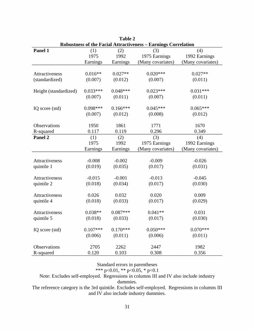
specifications in Table 1. Nevertheless, as shown in the top panel of Table 2, including height
has only minor effects on the estimated correlation between facial attractiveness and earnings.
Height also has very little effect on other estimated coefficients in the empirical model (the
results are not shown, but are available on request). The magnitude of the facial attractiveness
coefficient is roughly half the size of the height premium when only IQ and height are included
in the empirical models, and the facial attractiveness and height premia are similar when the
lengthy set of covariates are included.
Mocan and Tekin (2010) emphasize that ugliness may be a hindrance rather than beauty
being valuable. Hamermesh and Biddle (1994) also note, in 2 of 3 datasets they examine, that
while attractive people are paid more, “the premia for good looks are considerably smaller than
the penalties for bad looks and they are not statistically significant.” In the bottom panel of
Table 2, we break beauty into quintiles, with quintile one being the portion of the population in
the bottom 20th percentile of the facial attractiveness distribution. The WLS results are striking.
There appears to be no ugliness/plainness penalty for those in the bottom quintile of the
15 The estimates for facial attractiveness for women, after restricting the sample to women working 35 to 70 hours a week, are 0.005 in a regression analogous to column (1), and 0.048 (and significant at 1 percent) in a regression analogous to column (2). Including covariates, as done in columns (3) and (4) result in coefficients of 0.059 and 0.053 (both significant at 1 percent). All results not included in tables are available for the authors on request.
12
attractiveness distribution. Rather, there is a substantial, significant attractiveness premium for
those in the top quintile, particularly in the preferred specifications shown in columns (1) and
(2).16
Having multiple assessments of a respondent’s facial attractiveness is important for
understanding the results in Tables 1 and 2, particularly in the context of the prior literature. If
we estimate the column 3 empirical model 10,000 times when in each draw we take one random
coder of the available 12 attractiveness assessments, we get coefficients ranging from -0.006 to
0.039. The mean estimate is 0.012, or 40 percent smaller than the preferred estimates in Table 1.
The attractiveness estimate is significant at the 5 percent level only 62 percent of the time when a
single assessment is used.17 When a single assessment is used and we split attractiveness into
quintile indicators, we find the average ugliness penalty is larger than the top-quintile premium
(specifically, the average coefficient in the lowest attractiveness quintile is -0.019 and the
average coefficient is 0.013 in the highest). The lowest quintile estimate is significant roughly
twice as frequently at 5 percent (roughly 16 percent of the time) than the highest quintile
indicator. This raises the possibility that cross-coder variation may play some role in prior
findings of a substantial unattractiveness penalty.
III. The Source of the Earnings Premium Associated with Facial Attractiveness
The literature provides several explanations for a beauty premium in earnings. Harper
(2000), who found a penalty for plainness using the British National Child Development Study,
16 The attractiveness premium disappears in 1992 when we break attractiveness into quintiles and condition on the extensive set of characteristics – some of these may be affected by attractiveness. In the next section we examine factors that may account for the attractiveness premium. 17 In marriage markets one might think that the maximum of the attractiveness scores might be particularly important, since people are matching with only a single mate (though an average score might be a better indicator of the arrival rate of potential suitors). In labor markets, the extreme minimum and maximum scores may be less salient than the average. We find the average and maximum score behave similarly in 1975 and 1992, while the correlation between the minimum score and earnings is positive, but smaller in magnitude and insignificant. The standard deviation of beauty is also insignificantly correlated with earnings once the average level of beauty is included in the specification.
13
attributed the bulk of the pay differential to general employer discrimination. Biddle and
Hamermesh (1998) argue that customer discrimination, either driven by pure taste discrimination
or the (correct) belief that attractive attorneys are more effective than other attorneys in front of
judges and juries, explains the beauty premium among lawyers. Consistent with the idea that the
beauty premium may reflect true productivity differences, Reingen and Kernan (1993) describe a
series of personal selling experiments that show customers respond more favorably to physically
attractive salespeople. Landry et al. (2006) also found attractive female solicitors were more
effective in collecting contributions for a charitable organization in a door-to-door fund-raising
field experiment. Hamermesh and Biddle (1994) raise a number of possible ways that
attractiveness may affect earnings, but write “The strongest support is for pure Becker-type
discrimination based on beauty and stemming from employer/employee tastes.” Ruffle and
Shtudiner (2010) show, based on a field experiment in Israel, that attractive men were over twice
as likely as identically qualified plain men to get called back in response to a job application.
The most detailed inquiry into the source of the beauty premium comes from Mobius and
Rosenblat (2006), who find a sizeable beauty premium in an experimental labor market. In their
experiment, the “visual interaction channel,” where attractive people are perceived as being more
productive, and an “oral interaction channel,” where attractive people receive a wage premium
based solely on an anonymous telephone interview, each account for 40 percent of the pay
differential. The remaining 20 percent is attributed to higher confidence of attractive people: the
attractive simply believe they are more productive than others even when, as a group, they are
not. The visual interaction channel described by Mobius and Rosenblat is consistent with
Jackson et al. (1995) and many other studies in psychology that suggest attractive people will be
viewed as being more competent than those with average looks. Moreover, this effect will be
14
stronger when a direct measure of competence is absent than when it is present. What is striking
about the Mobius and Rosenblat results is that attractive people were no more productive than
others – the task being compensated was solving a maze – but beauty was rewarded by 12 to 17
percent higher compensation for a one-standard deviation increase in attractiveness. Thus,
Mobius and Rosenblat point to statistical discrimination that is unrelated to true productivity to
explain the attractiveness premium.
The WLS data open up new possibilities for investigating the reasons why there is a durable
earnings premium for facial attractiveness. The results from a series of empirical models
described below are consistent with facial attractiveness being an intrinsically valuable labor
market characteristic.
a. The attractiveness premium: it does not appear driven by cognitive skills or health
The most direct way that facial attractiveness might be linked to earnings would be if those
with greater facial attractiveness had better cognitive skills. Case and Paxson (2006), for
example, show across several datasets that there is a positive correlation between height and IQ.
A more subtle but related mechanism is suggested in the psychology literature, where it is
conjectured that teachers in K-12 schools give preferential treatment to attractive children.18
Hence, it might be the case in observational data that there is no link between attractiveness and
ability, but attractive children nevertheless have higher class rank than otherwise identical but
less attractive peers. This could lead to more total years of education or labor market
opportunities that are not available to their peers.
We examine these potential links estimating the correlation between facial attractiveness
and attributes mentioned above: IQ, high school class rank, and years of completed schooling.
In bivariate regressions, the correlation between attractiveness and IQ is 0.029 (with a standard 18 An early paper along these lines is Clifford and Walster (1973).
15
error of 0.017), significant at the 10 percent level. It is negatively but insignificantly correlated
with class rank -0.212 (0.246) and insignificantly correlated with educational attainment 0.015
(0.042). When we include family background measures there is no evidence that facial
attractiveness is positively, significantly correlated with IQ for males or with class rank: there is
no evidence that teachers bestowed advantage on attractive males, at least in this cohort of
Wisconsin students. Facial attractiveness is also not correlated with total years of schooling.
This fact is at least mildly surprising. Given there is an attractiveness premium, one might
expect attractive men to try to further exploit this labor advantage by acquiring additional human
capital.
Another possibility is that facial attractiveness is correlated with health. Healthy people
may command a labor market premium relative to otherwise identical workers, if only because
they have fewer work absences and have lower health insurance costs (Bhattacharya and
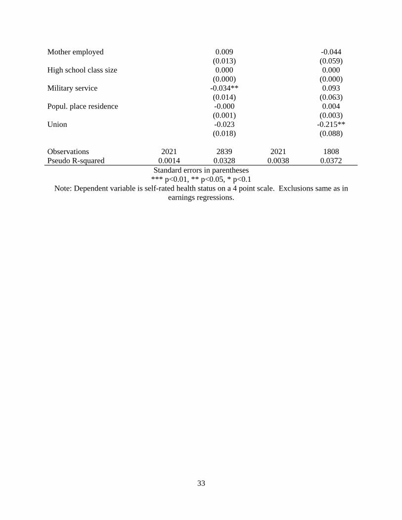
Bundorf, 2009). We examine two measures of health: mortality and self-reported health on a 4-
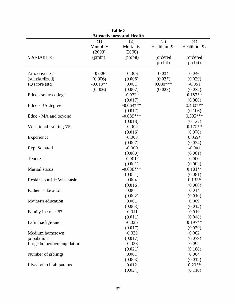
point scale (poor, fair, good, and excellent).19 In columns 1 and 2 of Table 3, we examine
correlates of mortality (marginal effects from the probit regression are reported in the table).
Three factors are significantly (at least at the 10 percent level), negatively correlated with
mortality: IQ, family income when in high school, and having a farm background. Facial
attractiveness in high school is uncorrelated with mortality. There is also no relationship
between facial attractiveness and self-reported measures of health in the ordered probit
regressions shown in columns 3 and 4.
To summarize, there does not appear to be any link between facial attractiveness and
measures of cognitive skills or health. Attractiveness is not positively, significantly correlated
19 In 2008 the WLS sample was matched to the National Death Index. 16.8 percent of the sample has died by 2008, when the typical WLS respondent was 68.
16
with IQ once family background is accounted for, with class rank, with total years of educational
attainment, with mortality, or with self-reported health status.
b. The attractiveness premium: the “visual interaction” channel and employer discrimination
Given we find no evidence for a direct link between attractiveness and cognitive ability,
there are four remaining broad explanations for the beauty premium. The first suggests that
others attribute characteristics to attractive people that they may or may not possess (the so-
called visual interaction channel). But if (perhaps mistaken) beliefs persist about the superior
productivity or communication skills of attractive people, they can earn more in the labor market
than their less attractive peers. The second holds that employers may simply choose to
discriminate by paying attractive men more than otherwise identical less attractive men. The
third suggests suggest that attractive people have better early-in-life experiences, confidence,
personality, and other skills than less attractive people and these attributes are productive in the
labor market. The fourth is that attractiveness itself enhances productivity in the labor market.
In this subsection we comment on the first two of these explanations.
The persistence of the attractiveness premium in Table 1 provides indirect evidence on the
visual interaction channel in observational data. It is not difficult to imagine that those with
physically appealing characteristics may receive higher initial compensation, but over time,
employers can observe true productivity. As in Farber and Gibbons (1996) and Altonji and
Pierret (2001), one would expect to see the effect of observable characteristics on earnings, such
as race or beauty, to become less important as true productivity can be observed, if race or
beauty is not correlated with true productivity after conditioning on other observable
characteristics.
We provide additional evidence on the durability of the beauty premium using WLS data on
17
job tenure. Specifically, we estimate the empirical models in Table 1, but add an interaction
term between facial attractiveness (and IQ) and tenure on the current job. Following the intuition
of Farber and Gibbons (1996) and Altonji and Pierret (2001), if employers are engaging in
statistical discrimination by assuming attractive men are more productive than less attractive
employees (who are otherwise observationally equivalent), then the correlation of attractiveness
and earnings should diminish with tenure on the job, and the correlation between measures of
true ability, such as IQ, should increase.
Table 4 presents evidence on this idea. Column 1 shows earnings in 1975 with tenure
interacted with facial attractiveness and IQ. Column 2 shows a similar specification for earnings
in 1992. By 1992 the interaction coefficients have the anticipated signs (positive for IQ*tenure,
and negative for beauty*tenure), though none of the tenure interactions are statistically or
economically significant.20 Though the evidence base for this conclusion is not overwhelming,
we do not see evidence in the WLS that supports the “visual interaction channel” explanation for
the facial attractiveness premium.
A favored explanation from early papers on the beauty premium is employer discrimination.
As Heckman (1998) notes, “Discrimination can persist in the long run, as long as entrepreneurs
with profitable opportunities choose to spend their money on discrimination.” We cannot rule
out the possibility that earnings are higher for attractive males relative to others simply because
profitable employers choose to pay attractive men more. We would find it puzzling that earnings
fail to reflect underlying productivity over the entire career of attractive men and the premium
appears independent of tenure with a given employer. We are particularly skeptical of this
explanation given results in the next subsection on links between attractiveness and high school
20 Recall, however, that this is a cohort dataset, so men in the sample have similar total years of labor market experience (though tenure with a given employer certainly differs across individuals).
18
experience, confidence, and personality. We nevertheless acknowledge that employer
discrimination could explain a portion of the attractiveness premium.
c. The attractiveness premium: high-school experiences, confidence, and personality
There are few occupations where height is an obvious productivity-enhancing attribute, but
Persico, Postlewaite, and Silverman (2004) and Case and Paxson (2006) document a height
premium in earnings. Persico et al. raise the possibility that tall children in K-12 school have
disproportionate access to leadership-building activities that are remunerative in later careers.21
Mocan and Tekin (2010) also point to experiences in K-12 schools as being the factor likely
explaining the results of their study of criminality: they conclude “the level of beauty in high
school has an effect on criminal propensity seven or eight years later, which seems due to the
impact of the level of beauty on human capital formation.”22 The WLS data, by having a high-
quality measure of IQ and a rich set of high school activities, provide an ideal opportunity to
look at links between facial attractiveness and high school experiences beyond class rank.
High school experiences
In Table 5 we present empirical models examining correlates of participation in varsity
sports (column 1), participation in student government (column 2), participation in service
organizations (column 3), and the total number of high school activities (column 4) for male
respondents.23 We include only family and community background characteristics in the
empirical models that were predetermined at the time WLS respondents were in high school. We
estimate columns 1-3 with probit regression (marginal effects are reported in the table). Column
21 As noted elsewhere, Case and Paxson argue that height is correlated with ability and has little independent effect on earnings. 22 The Mocan and Tekin results apply only to females, however. 23 Our social participation measures were also coded from high school yearbooks. The yearbooks were searched for any occurrence of the respondent’s name. When a match was found, the nature of the corresponding activity was coded into sports teams, pep activities, performance activities, subject clubs, etc. Yearbooks were coded for about 90 percent of the WLS sample.
19
1 shows that facial attractiveness is strongly, positively correlated with participation in varsity
sports for high school males. There is no a priori reason to think that facial attractiveness has
any innate relationship to athletic ability. Rather, we conjecture that handsome young men get
signaled out by coaches for extra attention when playing youth sports. Note that IQ has no
relationship, positive or negative, with participation in varsity sports. Similarly, facial
attractiveness is strongly correlated with participation in student government and the total
number of high school activities. As argued by Persico et al. (2006), high school activities may
enhance leadership skills, develop discipline and interpersonal skills that are valuable in adult
labor markets. Our results are consistent with the Persico et al. (2006) and Mocan and Tekin
(2010) evidence – facial attractiveness in high school appears to convey benefits to students that
may have a lifetime payoff.
The correlations between facial attractiveness and high school activities, while fairly strong,
do not fully explain the attractiveness premium in earnings, however. Table 6 repeats the
empirical specifications in Table 1 but includes indicators for participating in varsity sports,
student government, and a count of the total number of high school activities. These covariates
reduce sharply the magnitude (and significance) of the attractiveness premium in 1975, but has
no effect on the premium in 1992 (in fact, the coefficient estimates are larger). We nevertheless
think these results explain a piece of the attractiveness premium puzzle.
Confidence
Confidence plays a key role in generating the wage premium documented in the
experimental labor market described in Mobius and Rosenblat (2006). Attractive people were
more confident, which accounted for 20 percent of their wage premium. Attractive people also
did substantially better in a telephone interview (where their appearance could not be judged),
20
which accounted for an additional 40 percent of the wage premium. We suspect heightened
confidence played a role in the superior communication skills of attractive participants.
Confidence may also be a channel through which high school experiences result in improved
labor market performance.
The WLS includes proxy variables related to confidence. We focus on two composite
measures, one for “self acceptance,” and the other for “purpose in life.”24 Facial attractiveness is
strongly, significantly correlated with both measures. We then include these covariates in a
specification analogous to Table 1: results are given in Table 7. As with high school activities,
the proxy measures for confidence are generally positively, marginally significantly correlated
with earnings. Relative to the results in Table 1, they reduce the size and significance of the
coefficients in the specification where we condition only on IQ and the confidence measures. If
confidence is a personality trait, then it is not clear that we want to condition on the extensive set
of covariates included in columns 3 and 4, since these factors may be influenced by confidence.
Nevertheless, the results in columns 3 and 4 suggest that the greater confidence of attractive men
does not fully explain the attractiveness premium in earnings.
The “Big 5” Personality Traits
24 The underlying questions for “self acceptance” are “To what extent do you agree that you feel like many of the people you know have gotten more out of life than you have?” “To what extent do you agree that, in general, you feel confident and positive about yourself?” “To what extent do you agree that when you compare yourself to friends and acquaintances, it makes you feel good about who you are?” “To what extent do you agree that your attitude about yourself is probably not as positive as most people feel about themselves?” “To what extent do you agree that you made some mistakes in the past, but you feel that all in all everything has worked out for the best?” “To what extent do you agree that the past had its ups and downs, but in general, you wouldn't want to change it?” And “To what extent do you agree that in many ways you feel disappointed about your achievements in life?” The underlying questions for “purpose in life” are “To what extent do you agree that you enjoy making plans for the future and working to make them a reality?” “To what extent do you agree that your daily activities often seem trivial and unimportant to you?” “To what extent do you agree that you are an active person in carrying out the plans you set for yourself?” “To what extent do you agree that you tend to focus on the present, because the future nearly always brings you problems?” “To what extent do you agree that you don't have a good sense of what it is you are trying to accomplish in life?” “To what extent do you agree that you sometimes feel as if you've done all there is to do in life?” And “To what extent do you agree that you used to set goals for yourself, but that now seems like a waste of time?”
21
Recent papers have explored the relationship between personality and economic outcomes
(see, for example, Duckworth and Weir, 2010, and the overview paper of Borghans et al., 2008).
The WLS contains a 29-question abbreviated version of the 44-question big five personality”
inventory.25 Four dimensions – extroversion, agreeableness, conscientiousness, and openness –
are assessed with 6 questions. Neuroticism is assessed with 5 questions. Typical questions are
exemplified by the items used to assess extroversion, such as “To what extent do you agree that
you see yourself as someone who is full of energy?” Or “To what extent do you agree that you
see yourself as someone who tends to be quiet?” Respondents are asked to rate themselves on a
1 (agree strongly) to 6 (disagree strongly) scale for each of the various underlying questions.
The single-item responses are then coded into average scores.26
Table 8 shows the correlations between the WLS personality measures and attractiveness,
conditioning on a set of family background characteristics. Attractiveness is positively,
significantly correlated with extroversion, which reflects gregariousness, assertiveness, energy,
adventurousness, enthusiasm, and outgoingness. It is negatively, significantly correlated with
neuroticism, so attractive men are less tense, irritable, discontented, shy, moody, and are more
confident. Attractiveness is also positively correlated with conscientiousness and openness to
experience, though these correlations are significant at only the 10 percent level. We also find
IQ is strongly positively correlated with openness to experience, and strongly negatively
correlated with extroversion, agreeableness, and conscientiousness. It seems likely that
extroversion and emotional stability are valuable characteristics in the labor market. Hence,
25 Mueller and Plug (2006) describe the WLS personality measures and examine the links between personality and WLS earnings in 1992 for men and women. 26 Mueller and Plug (2006) report measures for Cronbach’s alpha reliabilities of 0.76 for extroversion, 0.71 for agreeableness, 0.66 for conscientiousness, 0.77 for neuroticism, and 0.60 for openness. Accounting for the smaller set of questions underlying the personality trait scores, the reliability ratings are very similar to those found in other datasets.
22
these correlations may help explain the attractiveness premium.
In Table 9 we repeat the specification in Table 1, but include the “big 5” personality traits.
As expected, extroversion is positively correlated with earnings as is emotional stability (the
absence of neuroticism). The big five personality traits, however, have relatively small effects
on the estimated attractiveness premium. In the specification that only includes IQ, the
magnitude of the coefficient is reduced by about one-third – from a 2 percent premium to 1.3
percent, in 1975, and from 3.2 percent to 2.3 percent in 1992. The precision of the estimates
falls as well, from estimates that are significant at 1 percent to estimates that are significant at 10
percent. When the lengthy set of characteristics, including family background, educational
attainment, household characteristics, and occupational choices are included, the magnitude and
significance of the attractiveness coefficient is essentially unchanged by including proxy
measures for the big-five personality traits. Consequently, while prior work has established a
relationship between personality traits and earnings, attractiveness appears to be a distinct factor
positively correlated with labor market earnings.
Can all measures together account for the attractiveness premium?
In Table 10 we combine the main high school experience measures, the confidence proxy
variables, and the summary big 5 confidence measures. The combined effect of these covariates
eliminates the attractiveness premium in 1975 earnings. Thus, we think at least a portion of the
attractiveness premium can be accounted for by its effects on high-school experiences, as
suggested by Persico, Postlewaite, and Silverman (2004) in the case of height; greater confidence
that attractive men have, as in experimental labor market described in Mobius and Rosenblat
(2006); and the ways that attractiveness and personality may interact. What is striking about the
Table 10 results, however, is that even accounting for the set of factors that largely account for
23
the attractiveness premium in 1975, attractiveness is positively, significantly (at the 10 percent
level) correlated with earnings in 1992. Moreover, the size of the estimated correlation is only
slightly smaller than the estimates in Table 1 when we do not account for these channels.
By process of elimination, we think there are two viable potential explanations for the
attractiveness premium for WLS males in their early 50s. The first, as mentioned earlier, is
employer discrimination, where profitable employers just choose to pay a premium to attractive
men. While we cannot definitely rule out this explanation, we think it is less compelling than the
competing explanation: attractiveness is an intrinsically productive characteristic in the labor
market. This may occur through superior communication or leadership skills or through other
channels. It is not fully accounted for by high school experiences, proxy measures of
confidence, or measures of the big 5 personality traits.
A striking WLS result provides indirect support for the idea that attractiveness is related to
intrinsic productivity: facial attractiveness of men is positively, significantly correlated with the
number of employers men have between 1975 and 1992. A household in the top 20 percent of
the facial attractiveness distribution has between 0.15 (with few covariates) to 0.18 (with
extensive covariates) more employers than men in the middle three quintiles of the attractiveness
distribution.27 While facial attractiveness is unrelated to job tenure in 1975, by 1992, facial
attractiveness is negatively, significantly associated with job tenure. Attractive men are
changing jobs more frequently than otherwise equivalent less attractive men. If employers were
simply willing to discriminate by paying an attractiveness premium, we would expect attractive
men to match with those employers and stay. Instead, it appears that attractive men exhibit
greater mobility in the labor market, where they move into jobs where their appearance
commands a wage premium. 27 The mean is 1.89.
24
IV. Conclusions
There is a durable, persistent economically large correlation between the facial
attractiveness of men, as measured by their high school yearbook photos, and their earnings in
their mid 30s and their early 50s. The magnitude and significance of the correlation is similar
whether we condition only on IQ or we condition on an extensive set of characteristics, including
family background, educational attainment, household characteristics, and occupational choices.
We are the first to document a long-run correlation between facial attractiveness and earnings.
One concern in interpreting our results is that attractiveness is measured in the WLS using
photos taken 18 and 35 years earlier than the observations on earnings that we study. While
longitudinal studies on the topic are scarce, the literature offers some insight into how
attractiveness evolves over time. As mentioned earlier, the general finding is that while facial
attractiveness declines with age from puberty onward, the relative ranking vis-à-vis peers is more
stable.28
The correlation between adolescent and middle-age beauty reported in the literature is
clearly not perfect. To explore how measurement error in the attractiveness variable might affect
our results, we take our actual attractiveness measure, a , and create an “updated” measure
2, where (0,1)
1updatea a Nρ σ σ
ρ= × +
−∼ and ρ is the assumed correlation between
attractiveness in high school and a later age. We estimate the 1992 regression with the
augmented list of covariates (the empirical model in column 4 of Table 1) taking 10,000 draws
for the “updated” attractiveness measure. We summarize the results below.
28 Neither facial expression nor orthodontic treatment seems to meaningfully change a person’s perceived attractiveness (Tatarunaite et al., 2005, and Zebrowitz, Olson, and Hoffman, 1993).
25
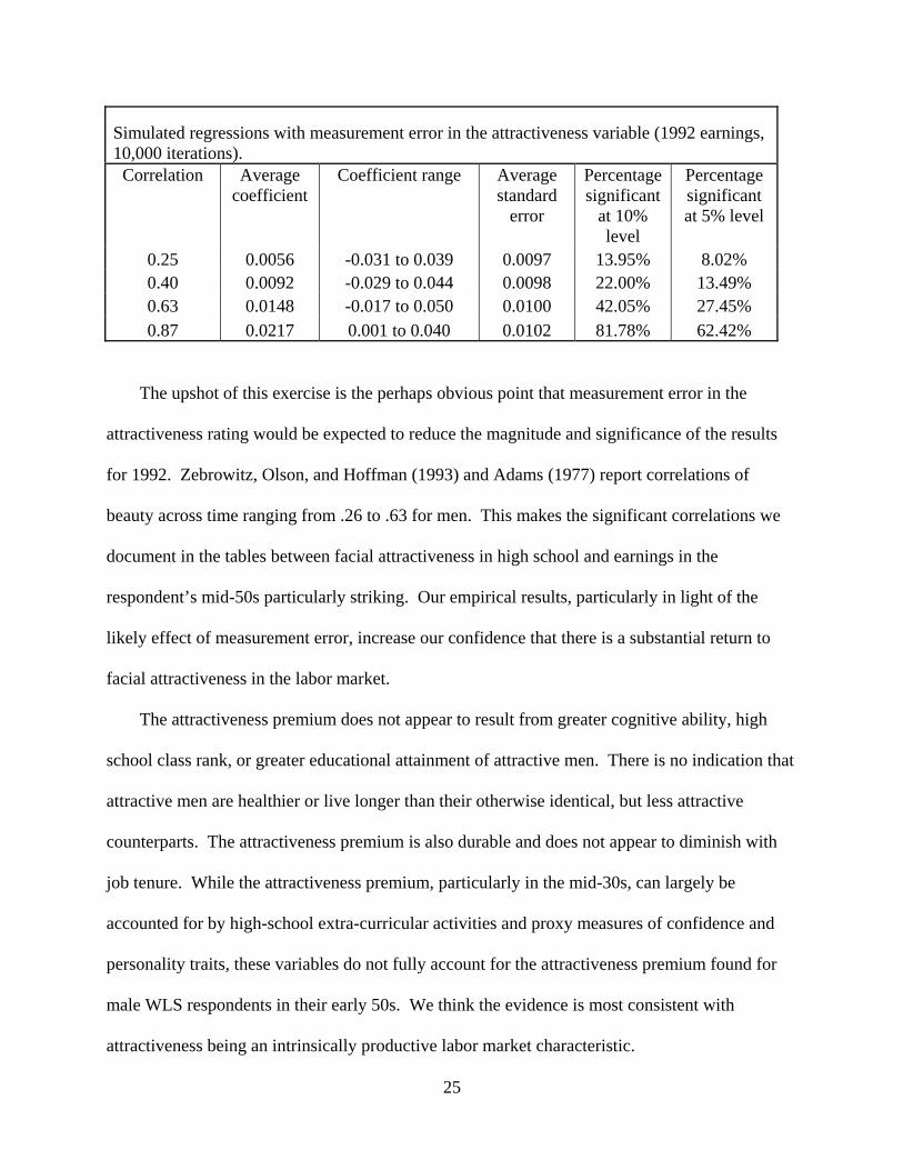
Simulated regressions with measurement error in the attractiveness variable (1992 earnings, 10,000 iterations).
Correlation Average coefficient
Coefficient range Average standard
error
Percentage significant
at 10% level
Percentage significant at 5% level
0.25 0.0056 -0.031 to 0.039 0.0097 13.95% 8.02% 0.40 0.0092 -0.029 to 0.044 0.0098 22.00% 13.49% 0.63 0.0148 -0.017 to 0.050 0.0100 42.05% 27.45% 0.87 0.0217 0.001 to 0.040 0.0102 81.78% 62.42%
The upshot of this exercise is the perhaps obvious point that measurement error in the
attractiveness rating would be expected to reduce the magnitude and significance of the results
for 1992. Zebrowitz, Olson, and Hoffman (1993) and Adams (1977) report correlations of
beauty across time ranging from .26 to .63 for men. This makes the significant correlations we
document in the tables between facial attractiveness in high school and earnings in the
respondent’s mid-50s particularly striking. Our empirical results, particularly in light of the
likely effect of measurement error, increase our confidence that there is a substantial return to
facial attractiveness in the labor market.
The attractiveness premium does not appear to result from greater cognitive ability, high
school class rank, or greater educational attainment of attractive men. There is no indication that
attractive men are healthier or live longer than their otherwise identical, but less attractive
counterparts. The attractiveness premium is also durable and does not appear to diminish with
job tenure. While the attractiveness premium, particularly in the mid-30s, can largely be
accounted for by high-school extra-curricular activities and proxy measures of confidence and
personality traits, these variables do not fully account for the attractiveness premium found for
male WLS respondents in their early 50s. We think the evidence is most consistent with
attractiveness being an intrinsically productive labor market characteristic.
26
References
Adams, Gerald. 1977. "Physical Attractiveness Research: Toward a Developmental Social Psychology of Beauty," Human Development, 20: 217-239.
Altonji, Joseph G. and Charles R. Pierret. 2001. “Employer Learning and Statistical Discrimination.” Quarterly Journal of Economics, February, 116(1), 313-350.
Becker, Gary S. 1973. “A Theory of Marriage: Part I,” Journal of Political Economy, August, 81(4), 813-846.
Bergstrom, Theodore C. and Mark Bagnoli. 1993. “Courtship as a Waiting Game,” Journal of Political Economy, February, 101(1), 185-202.
Bhattacharya, Jay and M. Kate Bundorf. 2009. “The Incidence of the Healthcare Costs of Obesity,” Journal of Health Economics, May, 28(3), 649-658
Biddle, Jeff E. and Daniel S. Hamermesh. 1998. “Beauty, Productivity, and Discrimination: Lawyers’ Looks and Lucre.” Journal of Labor Economics. January, 16(1), 172-201.
Borghans, Lex, Angela Lee Duckworth, James J. Heckman, and Bas ter Weel. 2008. “The Economics and Psychology of Personality Traits,” Journal of Human Resources, Fall, 43(4), 972-1059.
Borjas, George J. 1980. "The Relationship Between Wages and Weekly Hours of Work: The Role of Division Bias." Journal of Human Resources Fall, 15(3), 409-423.
Case, Anne and Christina Paxson. 2008. “Stature and Status: Height, Ability, and Labor Market Outcomes.” Journal of Political Economy, June, 116(3), 499-532.
Caspi, Avshalom and Brent W. Roberts. 1990. “Personality continuity and change across the life course,” in Handbook of Personality: Theory and Research, LA Pervin, OP John, Guilford Press New York.
Clifford, Margaret M. and Elaine Walster. 1973. “The Effect of Physical Attractiveness on Teacher Expectations,” Sociology of Education, Spring, 46(2), 248-258.
Duckworth, Angela Lee and David R. Weir. 2010. “Personality, Lifetime Earnings, and Retirement Wealth,” Michigan Retirement Research Center Working Paper, 2010-235, http://www.mrrc.isr.umich.edu/publications/papers/pdf/wp235.pdf (accessed 12/31/2010).
Farber, Henry S. and Robert Gibbons. 1996. “Learning and Wage Dynamics.” Quarterly Journal of Economics, February, 111(4), 1007-1047.
Feingold, Alan. 1992. “Good-Looking People Are Not What We Think.” Psychological Bulletin. March, 111(2). 304-341.
27
Hamermesh, Daniel S. and Jeff E. Biddle. 1994. “Beauty and the Labor Market.” American Economic Review. December, 84(5), 1174-1194.
Harper, Barry. 2000. “Beauty, Stature and the Labour Market: A British Cohort Study.” Oxford Bulletin of Economics and Statistics, Special Issue (62), 771-800.
Heckman, James J. 1998. “Detecting Discrimination.” The Journal of Economic Perspectives. Spring, 12(2), 101-116.
Hosoda, Megumi, Eugene F. Stone-Romero, and Gwen Coats. 2003. “The Effects of Physical Attractiveness on Job-Related Outcomes: A Meta-Analysis of Experimental Studies.” Personal Psychology. 56, 431-462.
Jackson, Linda A., John E. Hunter, and Carole N. Hodge. 1995. “Physical Attractiveness and Intellectual Competence: A Meta-Analytic Review,” Social Psychology Quarterly, June, 58(2), 108-122.
Landry, Craig E., Andreas Lange, John A. List, Michael K. Price, and Nicholas G. Rupp. 2006. “Toward and Understanding of the Economics of Charity: Evidence from a Field Experiment,” Quarterly Journal of Economics, May, 121(2), 747-782.
Langlois, Judith H., Lisa Kalakanis, Adam J. Rubenstein, Andrea Larson, Monica Hallum, and Monica Smoot. 2000. “Maxims or Myths of Beauty? A Meta-Analytic and Theoretical Review.” Psychological Bulletin. May, 126(3). 390-423.
Meland, Sheri A. 2002. “Objectivity in Perceived Attractiveness: Development of a New Methodology for Rating Facial Attractiveness,” M.A. Thesis: Department of Sociology, University of Wisconsin – Madison
Mobius, Markus M. and Tanya Rosenblat. 2006. “Why Beauty Matters.” American Economic Review, March, 96(1), 222-235.
Mocan, Naci and Erdal Tekin. 2010. “Ugly Criminals.” Review of Economics and Statistics, February, 92(1), 15-30.
Mueller, Gerrit and Erik J.S. Plug. 2006. “Estimating the Effect of Personality on Male and Female Earnings,” Industrial and Labor Relations Review, October, 60(1), 3-22.
Neal, Derek A. and William R. Johnson. 1996. “The Role of Premarket Factors in Black-White Wage Differences.” Journal of Political Economy. October. 104(5), 869-895.
Persico, Nicola, Andrew Postlewaite, and Dan Silverman. 2004. “The Effect of Adolescent Experience on Labor Market Outcomes: The Case of Height.” Journal of Political Economy. October, 112(5). 1019-1053.
28
Reingen, Peter H. and Jerome B. Kerman. 1993. “Social Perception and Interpersonal Influence: Some Consequences of the Physical Attractiveness Stereotype in a Personal Selling Setting,” Journal of Consumer Psychology, 2(1), 25-38.
Ruffle, Bradley J. and Ze’ev Shtudiner. 2010. “Are Good-Looking People More Employable?” Manuscript, Ben-Gurion University, November. http://papers.ssrn.com/sol3/papers.cfm?abstract_id=1705244
Sewell, William H., Robert M. Hauser, Kristen W. Springer, and Taissa S. Hauser. 2004. “As We Age: A Review of the Wisconsin Longitudinal Study, 1957-2001.” In Research in Social Stratification and Mobility, K.T. Leicht (ed), New York: Elsevier, 3-116.
Sicinski, Kamil. 2009. “Beauty and Marriage.” Chapter 2 of Ph.D. Dissertation in Economics, University of Wisconsin – Madison. 46-77.
Tatarunaite, Egle, Rebecca Playle, Kerry Hood, William Shaw and Stephen Richmond. 2005. “Facial attractiveness: A longitudinal study,” American Journal of Orthodontics and Dentofacial Orthopedics, 127(6), 676-682.
Zax, Jeffrey S. and Daniel I. Rees. 2002. “IQ, Academic Performance, Environment, and Earnings,” Review of Economic Statistics, November, 84(4). 600-161.
Zebrowitz, Leslie A., Karen Olson, and Karen Hoffman. 1993. “Stability of Babyfaceness and Attractiveness Across the Life Span,” Journal of Personality and Social Psychology, 64(3), 453-466.
29
Table 1
Attractiveness and Log Earnings of Men (1) (2) (3) (4) 1975
Earnings 1992
Earnings 1975 Earnings 1992 Earnings
Attractiveness (std) 0.020*** 0.032*** 0.020*** 0.026** (0.006) (0.011) (0.006) (0.010) IQ score (std) 0.107*** 0.171*** 0.050*** 0.070*** (0.006) (0.010) (0.006) (0.011) Educ - some college 0.077*** 0.197*** (0.020) (0.031) Educ - BA degree 0.257*** 0.484*** (0.023) (0.037) Educ - MA and beyond 0.308*** 0.594*** (0.028) (0.044) Vocational training '75 0.050*** 0.097*** (0.014) (0.025) Experience 0.018*** -0.015 (0.005) (0.012) Exp. Squared -0.000* 0.001** (0.000) (0.000) Tenure 0.006*** 0.009*** (0.001) (0.001) Marital status 0.130*** 0.176*** (0.017) (0.028) Resides out of WI 0.154*** 0.197*** (0.014) (0.024) Father's education -0.002 0.003 (0.002) (0.004) Mother's education 0.003 0.007* (0.002) (0.004) Family income '57 0.024** 0.048*** (0.010) (0.017) Farm background -0.001 0.029 (0.016) (0.028) Medium hometown pop. 0.021 0.068** (0.015) (0.027) Large hometown pop. 0.091*** 0.049 (0.022) (0.038) Number of siblings 0.006** 0.008* (0.002) (0.004) Lived with both parents -0.010 -0.015 (0.023) (0.040) Mother employed 0.010 -0.005
30
(0.012) (0.021) High school class size 0.000* -0.000 (0.000) (0.000) Military service 0.037*** 0.062*** (0.013) (0.022) Popul. place residence -0.001 0.002** (0.001) (0.001) Union -0.040*** -0.037 (0.013) (0.031) Constant 10.618*** 10.635*** 9.955*** 9.385*** (0.006) (0.011) (0.088) (0.200) Observations 2705 2224 2447 1982 R-squared 0.120 0.112 0.307 0.355
Standard errors in parentheses *** p<0.01, ** p<0.05, * p<0.1
Note: Excludes self-employed. Regressions in columns III and IV also include industry dummies.
31
Table 2
Robustness of the Facial Attractiveness – Earnings Correlation Panel 1 (1) (2) (3) (4) 1975
*** p<0.01, ** p<0.05, * p<0.1 Note: Excludes self-employed. Regressions in columns III and IV also include industry
dummies. The reference category is the 3rd quintile. Excludes self-employed. Regressions in columns III
and IV also include industry dummies.
32
Table 3 Attractiveness and Health
(1) (2) (3) (4) Mortality
(2008) Mortality
(2008) Health in ‘92 Health in ‘92
VARIABLES (probit) (probit) (ordered probit)
(ordered probit)
Attractiveness (standardized)
-0.006 (0.006)
-0.006 (0.006)
0.034 (0.027)
0.046 (0.029)
IQ score (std) -0.013** 0.001 0.088*** -0.051 (0.006) (0.007) (0.025) (0.032) Educ - some college -0.032* 0.187** (0.017) (0.088) Educ - BA degree -0.064*** 0.430*** (0.017) (0.106) Educ - MA and beyond -0.089*** 0.595*** (0.018) (0.127) Vocational training '75 -0.004 0.172** (0.016) (0.070) Experience -0.003 0.059* (0.007) (0.034) Exp. Squared -0.000 -0.001 (0.000) (0.001) Tenure -0.001* 0.000 (0.001) (0.003) Marital status -0.088*** 0.181** (0.021) (0.081) Resides outside Wisconsin 0.004 0.133* (0.016) (0.068) Father's education 0.001 0.014 (0.002) (0.010) Mother's education 0.001 0.009 (0.003) (0.012) Family income '57 -0.011 0.019 (0.011) (0.048) Farm background -0.025 0.197** (0.017) (0.079) Medium hometown population
-0.022 (0.017)
0.002 (0.079)
Large hometown population -0.033 0.092 (0.021) (0.108) Number of siblings 0.001 0.004 (0.003) (0.012) Lived with both parents 0.012 0.205* (0.024) (0.116)
33
Mother employed 0.009 -0.044 (0.013) (0.059) High school class size 0.000 0.000 (0.000) (0.000) Military service -0.034** 0.093 (0.014) (0.063) Popul. place residence -0.000 0.004 (0.001) (0.003) Union -0.023 -0.215** (0.018) (0.088) Observations 2021 2839 2021 1808 Pseudo R-squared 0.0014 0.0328 0.0038 0.0372
Standard errors in parentheses *** p<0.01, ** p<0.05, * p<0.1
Note: Dependent variable is self-rated health status on a 4 point scale. Exclusions same as in earnings regressions.
measure of neuroticism -0.001 -0.005 -0.000 -0.005 (0.002) (0.003) (0.002) (0.003) measure of openness 0.001 0.007** -0.001 0.004 (0.002) (0.003) (0.002) (0.003) IQ score (std) 0.100*** 0.151*** 0.058*** 0.071*** (0.009) (0.015) (0.010) (0.016) Educ - some college 0.083*** 0.219*** (0.029) (0.041) Educ - BA degree 0.241*** 0.508*** (0.033) (0.048) Educ - MA and beyond 0.252*** 0.566*** (0.040) (0.059) Vocational training '75 0.042** 0.067** (0.020) (0.031) Experience 0.015** -0.072*** (0.007) (0.018) Exp. Squared -0.000 0.002*** (0.000) (0.000) Tenure 0.005*** 0.009*** (0.002) (0.001) Marital status 0.108*** 0.165*** (0.027) (0.038) Resides outside Wisconsin 0.128*** 0.180*** (0.020) (0.031)
44
Father's education -0.005 -0.006 (0.003) (0.005) Mother's education 0.004 0.009* (0.003) (0.005) Family income '57 0.021 0.054** (0.014) (0.023) Farm background 0.026 0.032 (0.026) (0.041) Medium hometown population
0.051** (0.021)
0.088*** (0.034)
Large hometown population
0.126*** (0.032)
0.110** (0.050)
Number of siblings 0.006* 0.006 (0.003) (0.005) Lived with both parents -0.013 -0.027 (0.032) (0.051) Mother employed -0.004 -0.004 (0.017) (0.027) High school class size 0.000* -0.000 (0.000) (0.000) Military service 0.041** 0.093*** (0.019) (0.029) Popul. place residence -0.004** 0.004*** (0.002) (0.001) Union -0.061*** -0.072* (0.019) (0.042) Constant 10.276*** 10.304*** 9.654*** 9.834*** (0.106) (0.176) (0.178) (0.356) Observations 1299 1241 1178 1128 R-squared 0.161 0.175 0.323 0.403
Standard errors in parentheses *** p<0.01, ** p<0.05, * p<0.1
Note: Excludes self-employed. Regressions in columns III and IV also include industry dummies.
45
Appendix Descriptive Statistics of Important Variables
Collection Wave
Variable Mean SD Min Max N
1957 Attractiveness (std) 0.045 0.973 -2.734 2.856 39981957 Family income '57 (log, in 100's of nominal dollars) 3.929 0.687 0 6.906 37931957 Farm background 0.209 0.407 0 1 39981957 Female 0 0 0 0 39981957 High school class size 180.137 134.783 6 482 39981957 High school rank 97.303 14.632 61 139 37761957 In student government 0.149 0.356 0 1 29941957 In varsity sports 0.468 0.499 0 1 29941957 IQ 0.025 1.028 -2.661 2.984 39981957 Large hometown population 0.125 0.331 0 1 39981957 Medium hometown population 0.368 0.482 0 1 39981957 Total # of activities 3.516 3.103 0 19 29941975 Educ - BA degree 0.146 0.354 0 1 27051975 Educ - MA and beyond 0.165 0.371 0 1 27051975 Educ - some college 0.142 0.349 0 1 27051975 Experience 12.474 4.954 0 18 27051975 Father's education 9.786 3.207 4 17 26491975 Industry 6.354 3.243 1 12 27041975 Lived with both parents 0.912 0.283 0 1 27041975 Marital status 0.886 0.318 0 1 27021975 Military service 0.583 0.493 0 1 27051975 Mother employed 0.372 0.483 0 1 26991975 Mother's education 10.619 2.677 5 16 26801975 Number of siblings 3.153 2.498 0 26 27041975 People functions 0.726 0.446 0 1 26751975 Popul. place residence 1.214 3.823 0.001 78.949 25911975 Prefers business contact 0.19 0.392 0 1 26751975 Resides outside Wisconsin 0.305 0.46 0 1 27051975 Tenure 7.349 5.06 0 18.25 27031975 Union membership 0.39 0.488 0 1 27051975 Vocational training 0.197 0.398 0 1 27051975 Wages (log, in 1992 dollars) 10.625 0.323 9.584 11.566 27051975 Works in service industry 0.178 0.382 0 1 27041975 Years of education 13.872 2.439 12 20 27051992 Educ - BA degree 0.156 0.363 0 1 22231992 Educ - MA and beyond 0.19 0.392 0 1 22231992 Educ - some college 0.161 0.367 0 1 22231992 Experience 30.27 5.792 0 37 21971992 Feels positive & confident 5.255 0.893 1 6 1858
46
1992 Health status (self rating) 4.155 0.629 1 5 18691992 Height (std) -0.007 1.016 -5.479 4.829 18611992 Industry 6.6 3.311 1 12 22181992 Makes plans a reality 4.94 1.088 1 6 18591992 Marital status 0.857 0.351 0 1 22241992 Measure of agreeableness 27.63 4.432 8 36 17921992 Measure of conscientiousness 29.316 4.06 14 36 17841992 Measure of extraversion 22.449 5.253 6 36 17601992 Measure of neuroticism 15.274 4.681 5 29 17891992 Measure of openness 21.873 4.486 8 35 17561992 Number of employers 75-92 1.833 1.072 1 5 22211992 People functions 0.762 0.426 0 1 22141992 Popul. place residence 4.569 10.087 0.046 88.632 22151992 Prefers business contact 0.174 0.379 0 1 22141992 Purpose-in-life score 33.685 5.711 3 42 18661992 Resides outside Wisconsin 0.33 0.47 0 1 22241992 Self-acceptance score 32.85 6.016 2 42 18661992 Tenure 17.377 10.974 0.5 40 22121992 Union membership 0.137 0.344 0 1 22241992 Wages (log, in 1992 dollars) 10.654 0.523 8.987 12.206 22241992 Works in service industry 0.22 0.415 0 1 22181992 Years of education 14.111 2.506 12 20 22232008 Mortality status 0.12 0.325 0 1 2224
Note: All statistics are for men only. For the 1975 and 1992 collection waves the sample was further restricted to respondents that were not self employed and for whom earnings were not missing.


![Computational Photography - TU Wien · 7 Beautification [Deussen et al.] DataData--Driven Enhancement Driven Enhancement of Facial Attractiveness Tommer Leyvand, Daniel Cohen-Or,](https://static.documents.pub/doc/80x56/5b80fcee7f8b9aeb088e75cc/computational-photography-tu-wien-7-beautification-deussen-et-al-datadata-driven.jpg)


