Factor market distortion in China’s manufacturing industry Hang Gao * University of Leuven March 2013 Abstract Hsieh and Klenow (2009) link overall firm-level dispersions in marginal products to potential improvement of aggregate TFP in a monopolistic competition model. In this paper I extend their strategy on two counts. First, I decompose total distortions into systematic components and idiosyncratic residuals. Systematic components iden- tify the sources of distortion in the structure of factor markets, i.e. labour distortion across regions, capital distortions across segments and across sectors. Second, I mea- sure distortion components as the impact on aggregate output. Aggregate TFP used by Hsieh and Klenow (2009) fails to capture distortions across sectors. Measuring distortions in China’s manufacturing sectors from 1998 to 2007 elicits two important findings. The evolution of the measures shows clear reduction of labour distortion across regions and capital distortion across segments, but limited unwinding of capital misallocation across sectors. In addition, the large magnitude of the remaining dis- tortions in 2007 suggests policies to further reduce systematic distortions, especially for capital distortion across sectors. JEL codes: O4, R2, L5 Keywords: Productivity, Factor market distortion, China * I would like to thank Johannes Van Biesebroeck, Frank Verboven, and Joep Konings for helpful comments and suggestions. All remaining errors are my own. E-mail: [email protected].
Transcript
Factor market distortion in China’s manufacturing industry
Hang Gao∗
University of Leuven
March 2013
Abstract
Hsieh and Klenow (2009) link overall firm-level dispersions in marginal products
to potential improvement of aggregate TFP in a monopolistic competition model. In
this paper I extend their strategy on two counts. First, I decompose total distortions
into systematic components and idiosyncratic residuals. Systematic components iden-
tify the sources of distortion in the structure of factor markets, i.e. labour distortion
across regions, capital distortions across segments and across sectors. Second, I mea-
sure distortion components as the impact on aggregate output. Aggregate TFP used
by Hsieh and Klenow (2009) fails to capture distortions across sectors. Measuring
distortions in China’s manufacturing sectors from 1998 to 2007 elicits two important
findings. The evolution of the measures shows clear reduction of labour distortion
across regions and capital distortion across segments, but limited unwinding of capital
misallocation across sectors. In addition, the large magnitude of the remaining dis-
tortions in 2007 suggests policies to further reduce systematic distortions, especially
for capital distortion across sectors.
JEL codes: O4, R2, L5
Keywords: Productivity, Factor market distortion, China
∗I would like to thank Johannes Van Biesebroeck, Frank Verboven, and Joep Konings for helpful
comments and suggestions. All remaining errors are my own. E-mail: [email protected].
1 Introduction
As input growth slows down1 and the technology gap with advanced countries narrows2,
more efficient factor allocation becomes critical to develop the growth potential of China’s
manufacturing sectors. Product and factor market distortions squeezed out in the process
of economic transformation have promoted the aggregate productivity growth to some
extent, e.g. migration of surplus labour from low-productive agriculture to industry, and
joint-stock reform of state-owned banks. However, there remain some structural barriers
that hinder the further population movement across regions, such as the Hukou system
(Chan and Zhang, 1999). Since governments at various levels actively interfere in the
functioning of capital market, state-dominated banks often employ credit policies biased
towards urban state-owned firms or selective manufacturing sectors (Boyreau-Debray and
Wei, 2004). In contrary, product markets have become more integrated since the early
1990s when government took measures to remove the interregional trade barriers (Holz,
2009). Remaining output distortions might stem from local protectionism (Young, 2000),
size restriction (Guner et al., 2008) or geographical constraints on transportation costs.
All these market impediments systematically give rise to dispersions in labour and
capital productivity across firms. In this paper, I decompose firm-specific distortions
into a systematic part that is associated with misallocation in the structure of economy,
and a residual idiosyncratic part. Measuring the systematic distortions helps identify
the underlying sources and magnitude of factor market distortions and suggest policy
directions to improve economic efficiency. Hsieh and Klenow (2009) develop a theoretical
model to link overall firm-level dispersions in marginal products of labour and capital to
aggregate TFP. Using the same framework, I measure each component of distortions as
its impact on aggregate output.
Each systematic distortion subdivides the factor market into clearly identifiable seg-
ments. Factor immobility across segments incites disparity in factor returns. Suppressing
return differentials across segments would leave the remaining distortions in idiosyncratic
residuals within segments. Idiosyncratic residuals within segment are likely to involve oth-
er systematic distortions and a hypothetical random error. By normalizing idiosyncratic
residuals, I divide total labour distortions of each manufacturing sector into the systematic
1National Population and Birth Control Committee predicts that the size of Chinese population peaks
in 2033 and is quickly aging afterwards. On the other hand, manufacturing investment growth declines
9.8% in 2012. Higher labour costs or particular political pressures are shifting assembly lines of some
international manufacturing out of China, e.g. Nike and Apple.2China’s FDI outflows, part of which is used to procure western businesses for technology, brands and
know-how, increase rapidly from US$0.9 billion in 1991 to US$77.2 billion in 2012. Mergers and acquisitions
account for US$37.8 billion, or 49% of the total.
1
component across regions and the idiosyncratic component within regions. Capital dis-
tortions of each sector are separated into differentials between and within firm-segments,
where firms in each segment are exposed to similar financing cost of capital, e.g. big
state-owned enterprises (SOEs) in urban areas vs. small private businesses in rural areas.
Hsieh and Klenow (2009) assume different technology for each industry and aggre-
gate industrial TFP gains of total distortion reduction across manufacturing sectors using
Cobb-Douglas. Since aggregate TFP of each industry is linked to marginal product disper-
sions within the sector, aggregate manufacturing TFP used in Hsieh and Klenow (2009)
neglects measuring distortions across sectors and understates the potential economic effi-
ciency in full liberalization. I measure the distortion across sectors as the impact on aggre-
gate output, taking into account factor allocations across sectors. Government-directed
manufacturing investment makes capital distortion across sectors an important source of
systematic distortions in China.
In a similar framework, Brandt et al. (2013) construct province-level data and measure
the distortions across provinces and between state and nonstate sector with aggregate TFP,
assuming all sectors use technologies that have the same factor elasticities. My work differs
in three aspects. First, I use firm-level information. Capital segments categorize firms
in different level of ownership, urbanization, and size, rather than the simple state and
nonstate classification. Second, I additionally measure the systematic distortions across
sectors. Each industry is assumed to use different technology on production. Third, I
also measure the idiosyncratic distortions that are excluded in macro-data. Idiosyncratic
distortions incorporate policy distortions, random shocks and the remaining sources of
misallocation.
The evolution of the distortion measures reflects the improvement of allocative effi-
ciency. Using firm census data in China’s manufacturing sectors for period 1998-2007,
I find a clear reduction of labour distortion across regions and capital distortion across
segments. Within manufacturing sectors, labour distortion across regions and capital dis-
tortion across segments account for less than one-fifth of total labour and capital distortion
in 2007, but contribute to more than two-thirds of the total distortion reductions over the
period. In contrast, unwinding of the capital misallocation across sectors is limited.
The large magnitude of the existing systematic distortions indicates that improvement
of labour mobility across regions and capital mobility across segments and across sec-
tors is still important to promote overall economic efficiency. In 2007, about one-fifth of
total growth potential in efficient allocation is able to be achieved by eliminating these
systematic distortions. I investigate the dispersions in factor products across those three
dimensions and propose realistic policies, e.g. inland shift of labour-intensive manufactur-
2
ing, development of small credit markets, and a reduced role of government in financing
manufacturing sectors.
This paper is related to the literature that measures the effects of misallocation on
aggregate productivity. Early studies on misallocation in China examine the dispersions
in factor returns and provide insights of specific systematic distortions in factor markets.
Gong and Xie (2006) and Boyreau-Debray and Wei (2004) reveal low capital mobility
across the provinces in the 1990s. Zhang and Tan (2007) suggest that labour markets are
becoming more integrated, but capital markets have become more fragmented between
urban and rural and between farm and nonfarm sectors. Dollar and Wei (2007) highlight
the capital misallocation between state and nonstate sectors. In the studies that examine
the impact of other sources of misallocation on aggregate productivity, Restuccia et al.
(2008) and Vollrath (2009) analyze cross-country differences in aggregate TFP due to
the misallocation between agriculture and industry. Restuccia and Rogerson (2008) and
Bartelsman et al. (2009) assess the impact of idiosyncratic policy distortions in accounting
for cross-country differentials.
The rest of the paper is organized as follows. The next section illustrates the method-
ologies that decompose and measure distortions. In section 3, I will describe the micro-
level data set and approaches to calibrate the model parameters. Section 4 decomposes
total distortions into idiosyncratic and systematic components. Section 5 simulates the
counterfactual factor reallocations and offers policy implications. I conclude in section 6.
2 Methodology
2.1 Model
Hsieh and Klenow (2009) derive industrial aggregate TFP as a function of factor distortions
in a monopolistic competition model. I break down the total distortion into systematic
components and idiosyncratic residuals. All distortion components are incorporated into
aggregate output.
Following Hsieh and Klenow (2009), I assume the total output of economy Y aggregates
each industry i’s output Yi, (i = 1, ..., N), using a Cobb-Douglas technology:
Y =N∏i=1
Y θii , where
N∑i=1
θi = 1
Profit maximization implies PiYi = θiPY where P ≡N∏i=1
(Pi/θi)θi .
3
The industry output Yi itself is a CES aggregate of Mi differentiated products
Yi =
Mi∑j=1
Yσ−1σ
ij
σσ−1
Profit maximization yieldsYijYi
=(PijPi
)−σwhere Pi ≡
(Mi∑j=1
P 1−σij
) 11−σ
. The elasticity of
demand for Yij approximately equals −σ given very small share of one single firm in the
total industry.3
Each industry uses different technology to produce the differentiated products
Yij = AijLαiij K
1−αiij
Each firm j in industry i maximizes the profit
πij = PijYij −WLij
(1− τ li )(1− τ lir)(1− τ lij)− RKij
(1− τki )(1− τkis)(1− τkij)
which yields Pij = σσ−1
(W
αi(1−τ li )(1−τ lir)(1−τ lij)
)αi (R
(1−αi)(1−τki )(1−τkis)(1−τkij)
)1−αi1Aij
. Hsieh
and Klenow (2009) set constant W and R and infer the total distortion across firms from
the first order conditions of inputs. Here I allow a location specific wage W ir = W
(1−τ li )(1−τ lir)for region r in industry i and segment specific cost of capital Ris = R
(1−τki )(1−τkis)for segment
s in industry i. τ li and τki capture the distortions that marginal products of factor differ
across sectors. For instance, τki would be low for the industries that have easy access
to government aids, and high for industries with long payback period or long-term cash
flow. τ lir measures regional disparity of labour productivity. It would be low for inland
provinces and high for the coastal regions in China. τkis reflects the dispersion of capital
returns in different firm segments. It would be low for large state-owned firms, but high
for small private businesses. τ lij and τkij thus are the remaining idiosyncratic labour or
capital (relative to output) distortions.4 Those distortions bring about the dispersions in
marginal revenue product of labour and capital, i.e. MRPL and MRPK. First order
conditions of labour and capital give
MRPLij = αiσ − 1
σ
PijYijLij
=W ir
1− τ lij(1)
MRPKij = (1− αi)σ − 1
σ
PijYijKij
=Ris
1− τkij(2)
3The elasticity of demand for Yij is −ηij = −σ + Si(σ − ηi) ≈ −σ, where Si =PijYijPiYi
and ηi is the
elasticity of industry output Yi.4In the equivalent full settings, I separately define an output distortion together with pure labour and
capital distortions. maxLij ,Kij
{(1 − τyij)PijYij −
W ir
1−τl∗ijLij − Ris
1−τk∗ijKij
}Therefore, 1
1−τlij= 1
(1−τyij)(1−τl∗ij )
and 1
1−τkij= 1
(1−τyij)(1−τk∗ij )
.
4
Specific distributional assumptions of idiosyncratic distortions are required to separate
the systematic and idiosyncratic components, i.e. W ir and τ lij in (1), and Ris and τkij
in (2). Suppose average idiosyncratic distortions weighted by revenue are normalized
to zero for each sector-region and each sector-segment, i.e.∑
j∈r,j∈iτ lij
PijYij∑j∈r,j∈i
PijYij= 0 and∑
j∈s,j∈iτkij
PijYij∑j∈s,j∈i
PijYij= 0.5 Lir =
∑j∈r Lij and Ki
s =∑
j∈sKij aggregate demand of labour
in sector-regions and capital in sector-segments. W ir and Ris are solved as revenue-weighted
average MRPL in region r and MRPK in segment s respectively.
W ir =
σ − 1
σ
αi∑j∈r
PijYij
Lir
∑j∈r
(1− τ lij)PijYij∑
j∈rPijYij
=σ − 1
σ
αi∑j∈r
PijYij
Lir
=1∑
j∈r
1MRPLij
PijYij∑j∈r
PijYij
,MRPLir
Similarly,
Ris =σ − 1
σ
αi∑j∈s
PijYij
Kir
=1∑
j∈s
1MRPKij
PijYij∑j∈s
PijYij
,MRPKis
Idiosyncratic distortions τ lij , τkij can then be calculated from (1) and (2),
1
1− τ lij= αi
σ − 1
σ
PijYijW irLij
1
1− τkij= (1− αi)
σ − 1
σ
PijYijRisKij
Analogously normalizing systematic distortions within each industry i, i.e.∑rτ lir
∑j∈r
PijYij
PiYi=
0 for labour and∑sτkis
∑j∈s
PijYij
PiYi= 0 for capital, we have industrial weighted average
marginal products that are determined only by cross-sector distortions.
MRPLi ,1
Mi∑j=1
1MRPLij
PijYijPiYi
=W
(1− τ li )∑r
[(1− τ lir)
∑j∈r
PijYij
PiYi
∑j∈r
(1− τ lij)PijYij∑
j∈rPijYij
] =W
1− τ li
MRPKi ,1
Mi∑j=1
1MRPKij
PijYijPiYi
=R
1− τki
5Namely, Eir[τ lijPijYij
]= 0 and Eis
[τkijPijYij
]= 0.
5
Cross-region labour distortion τ lir and cross-segment capital distortion τkis can then be
solved as
1
1− τ lir=
MRPLir
MRPLi
1
1− τkis=
MRPKis
MRPKi
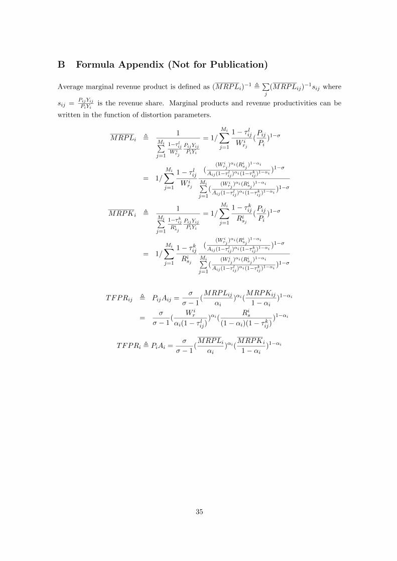
Now define revenue productivity for the firms and industry
TFPRij , PijAij =σ
σ − 1(MRPLij
αi)αi(
MRPKij
1− αi)1−αi
TFPRi , PiAi =σ
σ − 1(MRPLi
αi)αi(
MRPKi
1− αi)1−αi
We can calculate the aggregate TFP for the industry6:
Ai =Yi
Lαii K1−αii
=
Mi∑j=1
(Aij
TFPRiTFPRij
)σ−1 1σ−1
This equation translates the dispersions of revenue productivity into the aggregate TFP.
Revenue productivities are written as a function of distortion parameters. Reducing dis-
persion in marginal product for any improvement of distortions within sectors will lead
to a higher aggregate TFP. In this framework, firm productivity is taken exogenously
and does not vary with distortions. In the model specification we know firm productivity
Aij = κi(PijYij)
σσ−1
Lαiij K
1−αiij
where κi = (PiYi)− 1σ−1 /Pi is industry constant. Although it is not
directly observed, I can simply set κi = 1 as reallocation gains depend only on the ratios
of aggregate TFP and output change. We can also infer the price vs. quantity using the
assumed elasticity of demand. High real output is demanded when price is low. Hsieh
and Klenow (2009) simply proxy the real output Yij by (PijYij)σσ−1 , which equalizes the
demand factors across all the sectors.
2.2 Distortion Measures
Given any set of distortions W ir , R
is, τ
lij , and τkij , we obtain the unique competitive allo-
cations within and between the industries.7
Li =
Mi∑j=1
Lij = Lαiθi/MRPLi∑N
i′=1αi′θi′/MRPLi′
Ki =
Mi∑j=1
Kij = K(1− αi)θi/MRPKi∑N
i′=1(1− αi′ )θi′/MRPKi′
6See formula appendix for the derivation.7I do not show the formula of equilibrium allocation within the industries Lij/Li and Kij/Ki because
it is not used in the following calculations. Available upon request.
6
where L and K are aggregate supply of labour and capital.
For any improvement of distortions, I can calculate the aggregate output Y′
and com-
pare it with the actual level. All the industries’ outputs are aggregated with the unit
elasticity of substitution.
Y′
Y=
N∏i=1
(A′iL′αii K
′1−αii
AiLαii K
1−αii
)θiHolding the cross-sector distortions τi, eliminating overall within-sector distortions only
equalizes the marginal products of individual firms at the industrial average and does not
change factor allocations cross sectors. The increase of aggregate outputs then reproduces
the aggregate TFP gain of full liberalization in Hsieh and Klenow (2009):
A∗/A =
N∏i=1
Mi∑j=1
(A∗iAij
TFPRiTFPRij
)σ−1θiσ−1
where A∗i =Mi∑j=1
(Aσ−1ij
) 1σ−1
is the aggregate TFP for industry i when marginal products
are equalized across firms. Aggregating the ratios of A∗i /Ai across sectors in Hsieh and
Klenow (2009) thereby failed to capture the improvement of cross-sector allocative effi-
ciency8, but is appropriate to measure total within-sector distortions. Eliminating part
of the within-sector distortions could cause slight reallocation across sectors as industrial
average marginal revenue products vary in a function of distortion parameters.9
In my extension, I can calculate the counterfactual aggregate output of eliminating
any particular distortion and measure its contribution to the actual aggregate output.
Simultaneously eliminating τ lir and τ lij removes all the labour distortion in the industry
while eliminating τ lir itself only drops the regional disparity in marginal product of labour.
Accordingly, eliminating τkis excludes the segmental disparity in capital returns. Capital
distortions within sectors are rooted out when τkij is additionally removed. The dispersion
of marginal products or TFPR is lessened by either entirely or partially removing these
within-sector distortions, which increases the aggregate TFP of all the industries. The
most efficient TFP is achieved when we simultaneously wipe out all the within-sector
distortions τ lir, τlij , τ
kis and τkij . This is equivalent to the full liberalization case in Hsieh
and Klenow (2009). Additionally eliminating distortions across sectors τ li and τki results
in efficient allocation across sectors and reflects the largest economic growth potential for
allocative efficiency improvement.
8Hsieh and Klenow (2009) claim that cross-sector allocation are unchanged in full liberalization because
of the unit elastic demand. However, this implicitly assumes fixed aggregate output revenue.9See the formula appendix. Average of the remaining within-sector distortions weighted by the changed
revenue shares does not necessarily equal zero.
7
Borrowing the definition of Brandt et al. (2013), I measure distortions in log-points.
The overall distortion is measured as
D = ln(Y ∗/Y )
where Y ∗ is the aggregate output of full liberalization. Y is the actual aggregate output.
The advantage of this log-point measure is that it can be divided into additive distortion
components, e.g. ln(Y ∗/Y ) = ln(Y ∗/Ynwi) + ln(Ynwi/Y ) where Ynwi is the aggregate
output when all the within-sector distortions are eliminated. The first term measures
the cost of distortions across sectors from the efficient allocation. The second one is
the contribution of distortions within sectors. The disadvantage is that log-points might
understate the potential improvement of aggregate output for large magnitude.
I can measure regional labour distortion and segmental capital distortion within sectors
as the contribution of eliminating between- distortions to the actual aggregate output:
dbr = ln(Ynbr/Y )
dbs = ln(Ynbs/Y )
Corresponding idiosyncratic distortion measures are
dwr = ln(Ynwr/Y )
dws = ln(Ynws/Y )
Let Ynbr and Ynbs be the aggregate output when only between-region labour distortion or
between-segment capital distortion is eliminated. Ynwr and Ynws are the aggregate output
when there is no within-region labour distortion or within-segment capital distortion.
The alternative measures are to quantify the aggregate output losses (in log-points)
that existence of the distortions will beget from the factor market liberalization.
Dbr = ln(Y lnwi/Ynwr) and Dwr = ln(Y l
nwi/Ynbr)
Dbs = ln(Y knwi/Ynws) and Dws = ln(Y k
nwi/Ynbs)
where Y lnwi and Y k
nwi are the aggregate output eliminating all within-sector labour and
capital distortions respectively. Between- measures indicate the costs of the aggregate
distortions in factor market when factor returns within region or segment are equalized.
Within- measures are the costs of the remaining distortions when regional or segmental
disparity is removed.
Given the exogenous firm-level productivity, eliminating distortions across sectors does
not alter the aggregate TFP for each industry but could improve the allocation across
8
sectors and enhance aggregate output. I measure the effects of reallocation across sectors
as follows.
dlbi = ln(Y lnbi/Y )
dlbi = ln(Y knbi/Y )
Y lnbi and Y k
nbi are the total output when industrial average marginal products of labour or
capital are equalized.
Cost measures of the cross-sector distortions are
Dlbi = ln(Y l/Y l
nwi)
Dkbi = ln(Y k/Y k
nwi)
Y l and Y k are the aggregate output for eliminating all labour and capital distortions
respectively. Cost and contribution measures are exactly the same for the distortions
across sectors since they both improve from the actual sectoral allocation to efficient
allocation across sectors, i.e. Li = L αiθi∑N
i′=1
αi′ θi′
or Ki = K (1−αi)θi∑N
i′=1
(1−αi′ )θ
i′, with unchanged
aggregate TFP for each industry.
Measuring distortions using aggregate output especially for allocative efficiency across
sectors is somehow sensitive to the model specification. It relies on the Cobb-Douglas ag-
gregation of final output. Expenditure share on each industry is assumed to be fixed. This
appears to fit China’s manufacturing data well. Correlation of 4-digit sector shares in total
value-added between 1998 and 2007 is 0.83.10 Most of the manufacturing sectors share the
booming in the past ten years and it may be also foreseen for the next decade. Relaxing
the Cobb-Douglas aggregator alters the allocation equilibrium across industries.1112 In
a robustness check, I use a general CES function as a closer depiction of reality to test
distortions across sectors.
3 Data
I use the firm-level census data from 1998 to 2007 for all manufacturing sectors. It consists
of all the state-owned firms and nonstate firms with more than 5 million RMB revenue. The
10Correlation of sector shares in total value-added between 1998 and 2007 is 0.92 at 2-digit level.
11For a CES aggregator of final output, Y =
(N∑i=1
θiYφ−1φ
i
) φφ−1
, the allocation equilibrium is Li =
Lαiθ
φi P
1−φi /MRPLi∑N
i′=1
αi′ θφ
i′ P
1−φi′ /MRPL
i′
and Ki = K(1−αi)θ
φi P
1−φi /MRPKi∑N
i′=1
(1−αi′ )θ
φ
i′ P
1−φi′ /MRPK
i′.
12For a CES aggregator, I can still approximately aggregate gains of within-sector allocative efficiency,∑i θi ln(A∗i /Ai). However, it no longer matches the output change of eliminating total within-sector
distortions.
9
number of firms in census increases from slightly less than 150,000 in 1998 to over 310,000
in 2007. The variables include firm’s industry code, location, ownership, employment,
wage payment, value-added and capital stock. Hsieh and Klenow (2009) simply use the
fixed capital stock reported by firm at the original purchase prices. I follow the method
of Brandt et al. (2012) converting the book value of capital stock into the real values that
are comparable across time and across firms. Real capital stock is calculated using the
perpetual inventory method with a 9% depreciation rate and Brandt-Rawski investment
deflator.13
⇒ Insert Table 1 approximately here ⇐
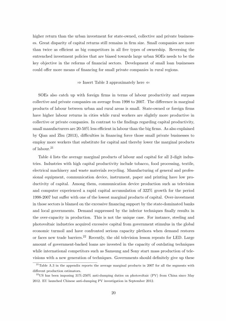
Table 1 provides the descriptive statistics on the underlying data set. Value-added and
output are translated into 1998 price level with a discount factor reflecting the factory
price indices of industrial goods. Input growth, i.e. 48% for employment and 111% for
fixed capital, is insufficient to explain the fivefold increase of value-added or output from
1998 to 2007. Using China’s industrial data for the same period, Brandt et al. (2012)
and Gan and Zheng (2009) both report an annual TFP growth of 8% on average. Most
of them seem to be attributed to the improvement of technical efficiency as Hsieh and
Klenow (2009) report only 2% per year TFP growth associated with better allocations of
resources. This suggests the considerable importance to investigate the systematic part of
total factor market distortions.
To estimate the effects of misallocation, I first need to pin down the key parameters of
the model, i.e. industry output share θi, industry labour share αi, and the elasticity of
substitution between firms σ. θi = PiYiPY is the industry share in total output revenue. But
since the model allows little room for the measurement error, I trim the top and bottom 1%
tails of labour and capital distortions and (revenue) productivity respectively within each
industry before calculating the shares. Hsieh and Klenow (2009) and Brandt et al. (2013)
set αi directly as the industrial labour share in the United States14, because the labour
share in China deviates from the labour production elasticity due to the distortions.15
Likewise, I map all NAICS industries into Chinese industry coding (CIC) and scale up
labour shares in US ASM data by 3/2 to take into account all the other fringe benefits
and Social Security contributions. Without the price information, I could not estimate
the elasticity of substitution per industry. The easy way is to set a conservative σ for all
13Brandt et al. (2012) provide an online appendix to describe all the methodology to construct the panel
data.14This implicitly assumes that labour shares in fixed costs covered by markup is the same as the labour
shares in variable costs.15Qian and Zhu (2013) find low correlation between labour income shares in China and in US using
alternative measures of labour share and explain the differentials by capital market distortions.
10
the industries, i.e. σ = 3 in Hsieh and Klenow (2009). A robustness check can be made
for a more aggressive σ.
I observe both employment and wage bills. Labour share as the wage bill over value-
added has a median only about 30% in the data set. So following Hsieh and Klenow (2009)
I assume a constant proportion of benefits added into wage such that total labour benefits
of all the firms in the sector equal 50% of aggregate value-added. One important issue is the
labour heterogeneity across firms. Employment in different firms could be quite different.
Wage per worker may vary within the region due to more the differences of work hours or
human capital than the rents shared by company. In the benchmark estimation, I measure
labour with normalized wage bill,WijLij∑rWijLij
Lir, to control for the labour heterogeneity
within the region. In a robustness test, I also measure labour simply using employment.
Labour between regions is perfectly substitutable in the same sector. This is not an
irrational surmise. Although the labour in Eastern regions could be better educated
than those in the West, the gap should not be wide especially for the manufacturing
sectors. Western workers are considered more hardworking than those from the East. The
longer working hours may fill in the small gap in quality. Workers are also assumed to
substitute across sectors. Labour differentials across sectors are simply ignored, which
might overestimate the labour distortion across sectors.
Regions are defined as 31 officially classified provinces excluding Hong Kong, Macau
and Taiwan. Segment category is the combination of 5 ownership types, urban/rural
classification and big/small firm size. Ownership includes state-owned, collective, private,
foreign-funded companies and Hong Kong, Macau and Taiwan (HMT) joint ventures.
Urban and rural classification depends on the administrative division. All the counties
are regarded as rural because of the high proportion of agriculture population while the
other county-level cities and municipal districts are treated as urban. Big firms have the
capital stock higher than the median in 4-digit industries. Observations are categorized in
425 4-digit CIC sectors in 2007. 2-digit CIC aggregation can further reduce the number
of sectors to 30.
⇒ Insert Figure 1 approximately here ⇐
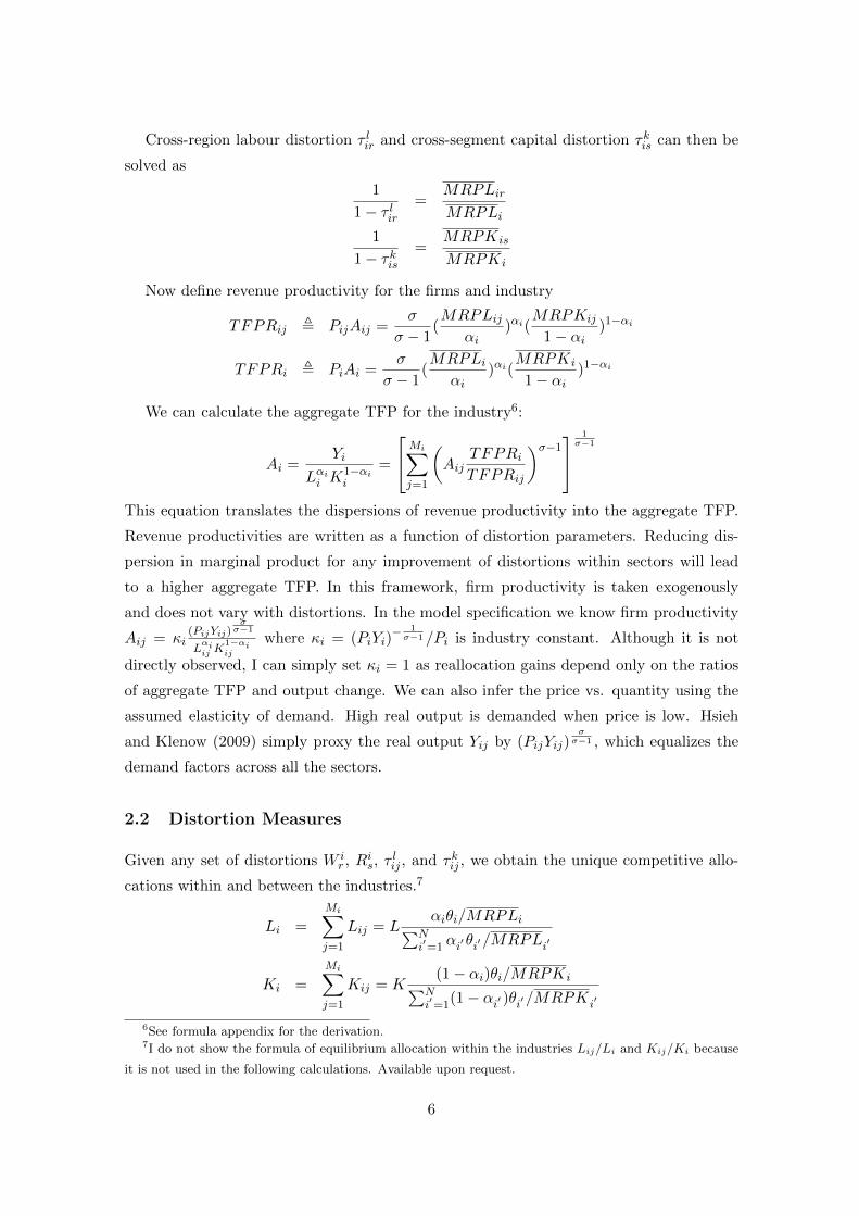
Figure 1 illustrates the input allocations by different firm types over the period. Fig-
ure 1(a) shows that most of the new jobs in manufacturing sectors are located in the
Eastern region that includes all the coastal provinces, whereas manufacturing employ-
ment slightly drops in Northeast, Middle and West. Since firms in the Eastern regions are
considered to have the highest labour productivity in the country, labour migration from
inland to coastal provinces could have mitigated distortions across regions and promote
11
the overall economic growth. Figure 1(b) shows that capital accumulation slightly rises
for state-owned firms but declines for collective companies. In contrast, private and for-
eign investment has experienced huge development. In 1998 SOEs dominate the economic
activities with 64% of total accumulated capital and 58% of total employment while in
2007 state-owned, collective/private, and foreign/HMT firms possess 45%, 21% and 34%
of total capital respectively and each provide about one-third of total employment. The
increase of private businesses is partly related with the privatization of SOEs. Lower
proportion of inefficient state-owned firms in economy could have improved the resource
allocations across ownership. Figure 1(c) shows that urban firms account for about 84%
of total capital in manufacturing sectors with 73% of total observations. Big firms provide
80% employment but 96% capital stock in total manufacturing. This might be associated
with the investment policies biased toward big urban companies. Allocative distortions
arise when big differentials in productivity exist between firms with different size in urban
or rural areas. Figure 1(d) shows that capital accumulation in metallurgy and equipment
manufacturing is more than 30% faster than the other industries in the period, i.e. met-
allurgy of 131%, equipment of 132% vs. chemistry of 99% and the other manufacturing
of 91%. Excessive financing support could create over-capacity and lower productivity in
those selective sectors. In section 5, I will investigate the differentials in marginal products
of input across 2-digit manufacturing sectors.
4 Distortion decomposition
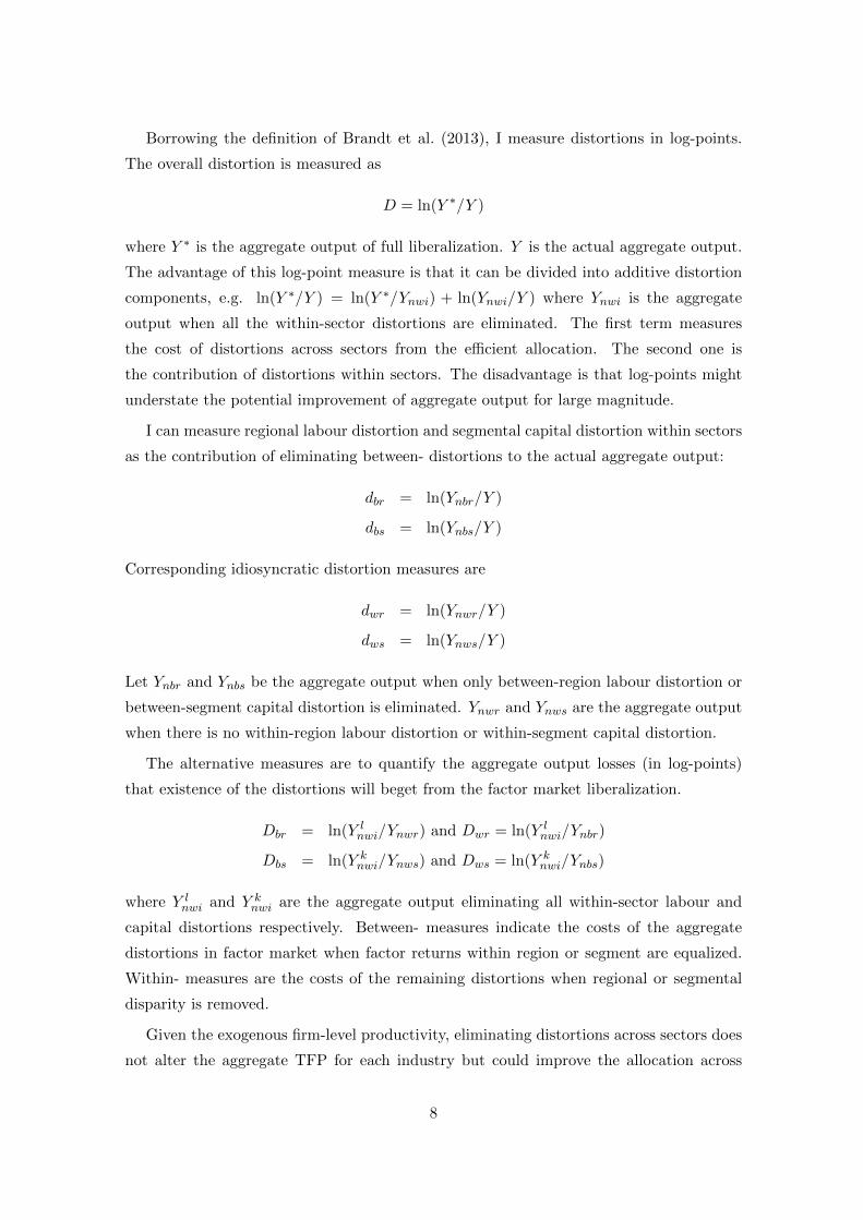
Figure 2(a) displays aggregate output gains (in log-points) associated with eradication of
total labour or capital distortions and full liberalization of both inputs over time. Overall
distortion drops dramatically in the beginning years and rise slightly at the end of pe-
riod. Eliminating total labour and capital distortions both significantly boost aggregate
output while the contribution of total labour distortion is a bit higher than that of total
capital distortion. Figure 2(b) and 2(c) plot the decomposition of total labour and cap-
ital distortions over time. Each component of distortion is measured as its contribution
to the actual aggregate output. The cost measures exhibit the same evolution patterns
but in slightly lower magnitude for within-sector distortions. Both measures coincide for
cross-sector distortions.
⇒ Insert Figure 2 approximately here ⇐
12
4.1 Misallocation within Sectors
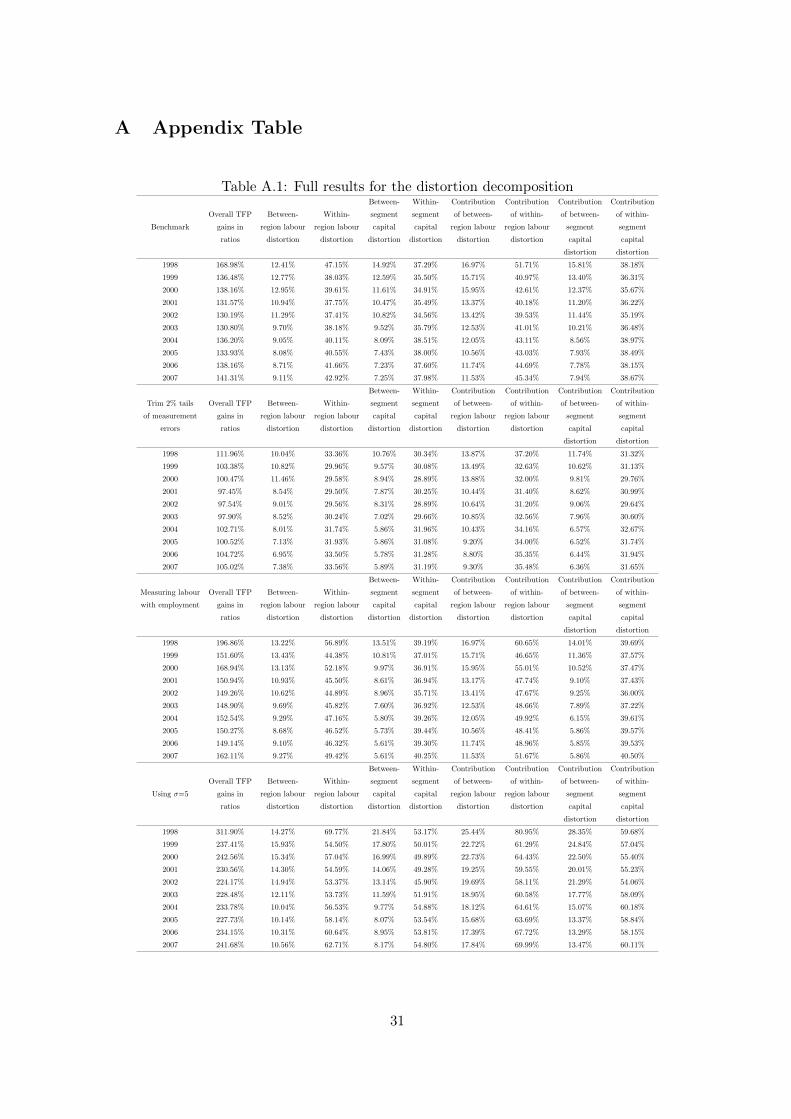
Hsieh and Klenow (2009) find that TFP gains (in change-ratios) of a full liberalization
within industries of China drop from 115.1% in 1998 to 86.6% in 2005, which gives an
allocative efficiency improvement of 15% (2.115/1.87), or 2% per year. I extend the data to
ten years’ period and obtain TFP gains of eliminating all within-sector distortions about
50% higher than reported by Hsieh and Klenow (2009), i.e. 169% in 1998, 130% in 2002,
134% in 2005, and 141% in 2007. These differentials in TFP gains are probably ascribed
to different industry composition or data truncation for measurement errors. My results
also infer 15% (2.69/2.34) within-sector allocative efficiency improvement from 1998 to
2005 but reveal a rise of TFP gains after 2002.
Figure 2(b) shows the evolution of labour distortions between and within regions in
the industries. In contrast to the between-region curve, idiosyncratic labour distortion
within regions is more than three times as large. Its reduction is slightly larger than
the fall of between-region distortion over the period, i.e. 6.3% vs. 5.5% in contribution
measures. However, within-region labour distortion exhibits a stable climbing after 2002
following a big drop in the first year. Between-region labour distortion takes a persistent
downward trend which is flattening after 2005. Population movement from interior to
coastal provinces has continuously reduced the labour distortion across regions. This
might also be associated with the national ”West Development Strategy” published in the
late 1990s to lessen regional imbalance in labour and capital productivity. Further labour
migration is meaningful as the between-region labour distortion at the end of period is
still significant, i.e. 9.1% in cost measure and 11.5% in contribution measure. In addition,
the greater TFP gain is able to be achieved by exploiting the big rising within-region
labour distortion. As τ lij also captures policy distortions on output markets, this might
be associated with the more government intervention in production.
Figure 2(c) depicts capital distortions between and within segments in the industries.
Idiosyncratic capital distortion within segments accounts for more than two-thirds of
total capital misallocation but the improvement of between-segment capital allocation
contributes to most of the capital distortion reduction between 1998 and 2007. Within-
segment capital distortion slightly increases while between-segment capital distortion is
roughly reduced by half in the decade. Deepening reforms of the financial system, i.e.
privatizing state-owned banks and developing stock and bond markets, are targeting for a
more efficient capital market where the gap of financing costs shrinks across firms of dif-
ferent types. The improvement of capital mobility across segments is still important as in
2007 between-segment capital distortion is 7.3% in cost measure and 7.9% in contribution
measure. Moreover, capital reallocation within segments might provide more potential
13
gains, e.g. the interprovincial imbalance of capital accumulation and efficiency.
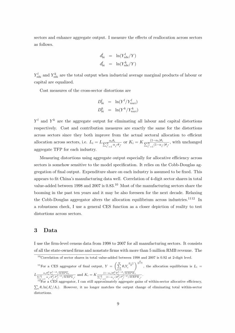
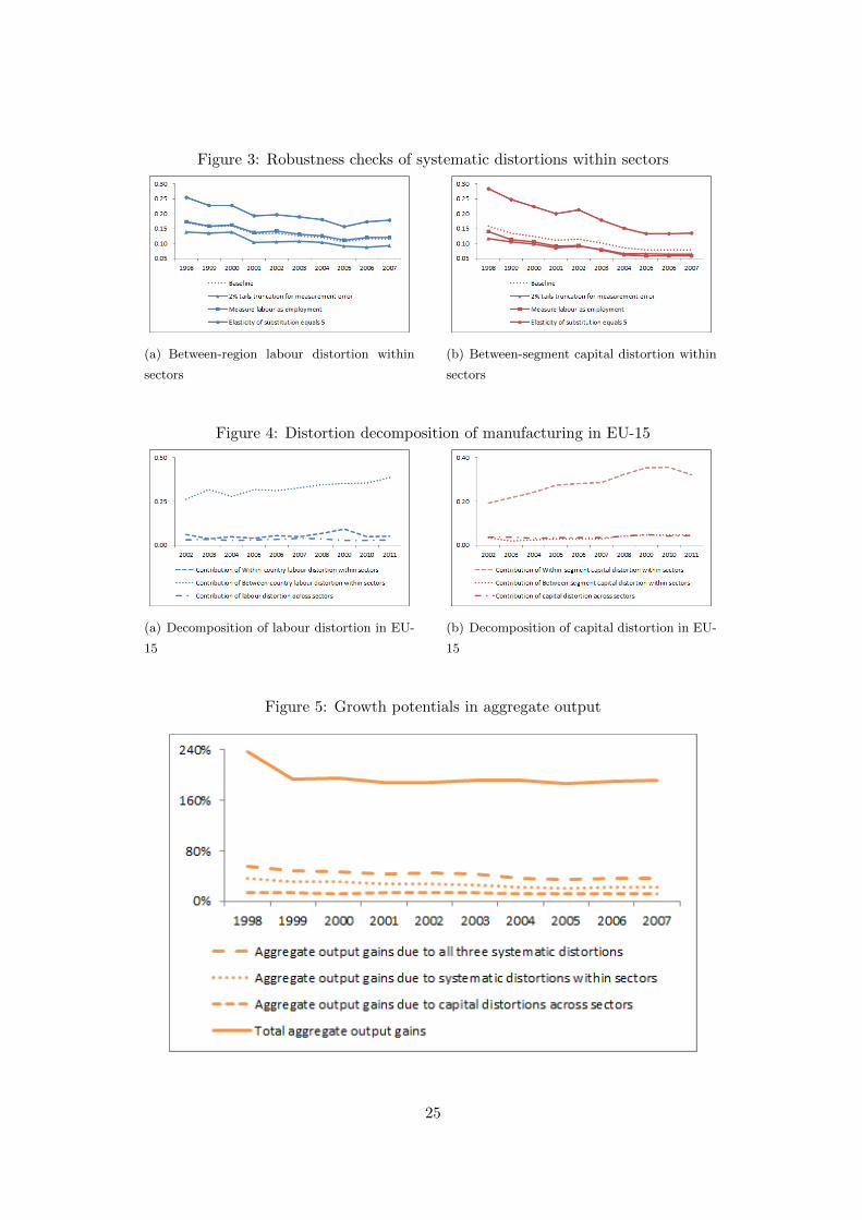
I perform three robustness checks on the distortion decompositions. All these ro-
bustness checks confirms rising idiosyncratic distortions and falling systematic distortions
within the sectors. In the end of data period, great economic growth is still able to be
achieved by eliminating the existing systematic distortions. Figure 3(a) and 3(b) illustrate
the evolution of systematic distortions within sectors for each robustness check.16
⇒ Insert Figure 3 approximately here ⇐
The framework of Hsieh and Klenow (2009) is vulnerable to measurement error. To
get rid of the possible outliers that enlarge the return dispersions within each industry, in
the benchmark results I trimmed top and bottom 1% tails of MRPL, MRPK and TFPR
which add up to 6% of total observations. Doubling the data truncation to 2% tails or
12% of observations lowers the total TFP gains from 169% to 112% in 1998 and from 141%
to 105% in 2007. Data of 1998 might have greater measurement errors in the remaining
1% tails than the other years. More importantly, the evolution of the distortions does not
differ from the benchmark results. Most of the reductions in TFP gains are reflected in
the idiosyncratic distortions. Idiosyncratic distortions are reduced by about one-fifth but
also show a rebound after 2002. The gains of eliminating systematic distortions within
sectors still follow a clear downward trend and end with 9.3% for labour and 6.4% for
capital in contribution measures.
To control for the labour heterogeneity within industries, I measure labour as the
normalized wage by assuming that the wage per worker differs only because of the work
hours and human capital. However, the more productive firms might be willing to share
the rents with workers and pay higher wages. Therefore, the benchmark results might be
underestimating the dispersion of marginal product of labour. Simply using employment
as the measure of labour input indeed raises the labour distortions. Since I assume the
perfect substitution of labour across regions, all the additional labour heterogeneity is
added into the idiosyncratic labour distortions within regions. Aggregate TFP gains of
eliminating overall distortions decline from 197% in 1998 to 162% in 2007, about 20%-
30% higher than the benchmark results. Neglecting the labour heterogeneity amplifies
the idiosyncratic labour distortion but still generates a similar pattern of evolution for all
distortion components.
I assume a constant elasticity of substitution for all industries, σ = 3. Hsieh and
Klenow (2009) address that this is conservatively at the low end of empirical estimates
16Table A.1 in the appendix reports the full results of the distortion decomposition for baseline model
and three robustness checks.
14
and when σ is higher, productivity dispersions are closed more slowly in response to the
efficient reallocation, enabling bigger gains from eliminating distortions. Full liberalization
TFP gains under σ = 5 skyrocket from 169% to 312% in 1998 and from 141% to 242%
in 2007. All labour and capital distortions soar as well by more than a half over the
benchmark results. In 2007, the contribution of within-sector systematic distortions is
17.8% for labour and 13.5% for capital.
Brandt et al. (2013) report the opposite findings that capital distortion between state
and nonstate sectors increases and labour distortion across provinces does not decline after
1998. However, they make a strong assumption that all the sectors use the same production
technology. As SOEs might have been shifting toward capital-intensive industries within
the manufacturing sector (Song et al., 2011), their result is likely to underestimate the
capital productivity of state sector and thereby overestimate the capital market distortions
in the recent years. In addition, they use aggregate non-agricultural data and argue that
the industry composition of the state sector has become slightly more labour intensive.
But the rising labour shares of the state sector actually stem from health, education and
government sectors rather than the manufacturing sectors.
4.2 Misallocation across Sectors
Figure 2 also measures the labour and capital distortions across sectors. They reflect
the inter-sector reallocation effects on aggregate output when industrial average marginal
revenue products of labour or capital are equalized. Since TFP of individual firms is
assumed to be exogenous in the model, aggregate TFP of each industry is not affected by
the distortions across sectors. However, in reality, capital distortions across sectors could
arouse over-capacity and lower TFP of the firms in some industries. Therefore, taking
individual productivity as an exogenous variable in the model is likely to underestimate
the reallocation effect across sectors on the aggregate output.
The evolution of cross-sector capital distortions reveals a limited improvement of capital
misallocation across sectors, i.e. 2.3% reduction from 1998 to 2007. Empirical studies
that investigate inter-sector reallocation effects in the real aggregate productivity growth
confirm the poor improvement of capital misallocation across sectors in China’s industrial
growth, e.g. Lin and Ge (2012) and Lu (2002) using the strategy of Syrquin (1984). More
importantly, capital distortion across sectors even has higher magnitude than between-
segment capital distortion within sectors at the end of period, i.e. 10.9% vs. 7.9% in
contribution measures. Excessive investment directed by the government over selected
sectors has negative impacts on inter-sector allocative efficiency. Large capital distortions
across sectors raise the importance of formulating policies to improve the capital mobility
15
across sectors, i.e. reducing the role of government in financing manufacturing industries.
Less than 1% reduction is found for labour distortions across sectors over the period.
Distortion measures have modest magnitude, i.e. 8.2% in 2007. However, I do not em-
phasize this source of misallocation based on two counts of concerns. First, as industries
cluster across provinces, labour distortion across sectors would mix up with part of re-
gional dispersions in labour productivity. This issue is less severe for capital as most of
the manufacturing sectors are open to alternative ownership. Second, industries require
different labour skills. Failure to identify the labour heterogeneity across sectors would
also overestimate the sectoral distortions on labour.
The robustness checks in the previous section hardly affect the distortions across sectors.
They are more sensitive to the Cobb-Douglas aggregation of sectoral outputs. However,
unobserved demand factor κi no longer cancels out in the change of CES aggregations.
Following Hsieh and Klenow (2009), here I ignore this cross-sector variations and simply
set κi = 1 for all the sectors. Suppose that final good is a CES aggregate of sector outputs:
Y =
(N∑i=1
θiYφ−1φ
i
) φφ−1
When sector outputs are more complementary (φ = 0.5), the contribution of capital
distortion across sectors becomes much smaller, i.e. 5.5% vs. 10.9% in 2007. Sectors with
high productivity obtain less capital in the reallocation. When sector outputs are more
substitutable (φ = 1.5), the contribution of capital distortion across sectors becomes much
larger, i.e. 16.6% vs. 10.9% in 2007. Since sector outputs are better substitutes, more
capital is reallocated toward the sectors with high productivity. CES aggregator of sector
outputs does not alter aggregate TFP gains of each industry. Within-sector distortion
measures slightly differ with the new cross-sector allocative equilibrium.
4.3 Comparison with EU-15
Another robustness check is to apply the same method on the developed countries that
are supposed to have less distortions on both product and factor markets. Brandt et al.
(2013) find that between-state distortions in the United States is significantly smaller
than between-province distortions in China. I compare my results of China with the
decomposed distortions in EU-15 countries.17
I extract all manufacturing firms in EU-15 countries from Amadeus database that
includes comprehensive company information across Europe. After trimming observations
17EU-15 refers to the first 15 Member States of the European Union before the new Member States joined
the EU after 2004. The 15 Member States are Austria, Belgium, Denmark, Finland, France, Germany,
Greece, Ireland, Italy, Luxembourg, Netherlands, Portugal, Spain, Sweden, and the United Kingdom.
16
with missing value in fixed assets, employment, wage bill and value-added, I obtain the
number of firms increasing from over 168,000 in 2002 to about 282,000 in 2011. Nominal
aggregate value-added grows 4.25% per year in the ten years’ period. Sectors are defined
at 4-digit NAICS.
Country/territory is the most important segment in EU labour market. Cultural and
language differences are major causes of worker immobility across borders. National sys-
tems that safeguard employment, e.g. long-term unemployment benefits, early retirement
packages, subsidized career break schemes and so on, encourage employees to stay put in
the country rather than looking for outside job. Benefits of purchasing houses with tax
breaks, interest subsidies and premium, and indirect tax of property sales provide other
disincentives to moving out of the country. With regard to capital segment, I combine
five types of ownership and four firm size categories. Amadeus database defines the ul-
timate owner as the largest owner in a firm with total or direct ownership of over 25%.
Following OECD (2006), I make a distinction of five different types of ultimate owners: (i)
state, when the ultimate owner is government or a public authority; (ii) family, when the
ultimate owner is either a family or an individual; (iii) industrial company; (iv) financial
company, when the ultimate owner is either a financial institute, an insurance company,
or a bank; and (v) other, when the ultimate owner does not exist or is one of the following:
employees/managers, foundation, or mutual pension fund/trust. All firms in Amadeus are
categorized into ’very large’, ’large’, ’medium sized’ and ’small’ groups, which account for
3%, 13%, 37% and 47% of total observations respectively.
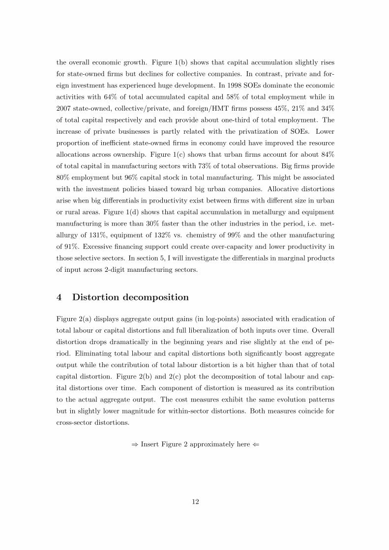
The contemporary total aggregate output gain due to distortions in EU-15 manufactur-
ing is only 50%-60% of that in China. The decomposition of labour and capital distortions
in EU-15 is reported in figure 4. Labour distortion across countries in EU of more than
25% is much larger than the between-province distortions in China (11.5%-17%). More-
over, it turns out to uprise after 2007. Manufacturing sectors in Southern Europe might
have suffered more in the global economic downturn. However, labour distortion within
countries contributes only about 5% of aggregate output loss and is roughly stable over
time. Figure 4(b) indicates that capital distortions across firm segments and across sectors
in Europe are significantly smaller than in China as expected. Both distortions exhibit
comparable magnitude persistently over the period. Eliminating each systematic capital
distortions only promotes the aggregate output by nearly 4%.
⇒ Insert Figure 4 approximately here ⇐
17
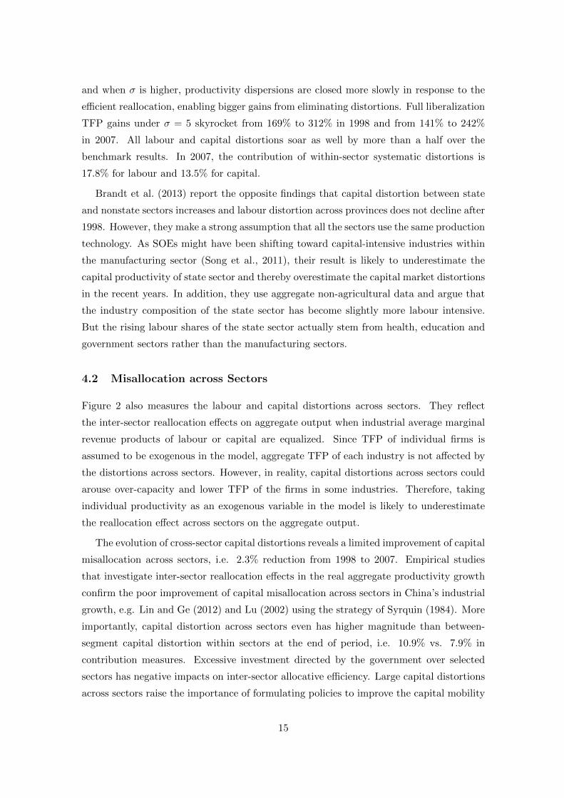
5 Policy Implication
Decomposition of total factor market distortions across different dimensions brings for-
ward important policy implications. In the previous section, distortion measures strongly
suggest further improvement of labour mobility across regions and capital mobility across
segments and across sectors. Figure 5 reports the potential aggregate output gains in
change-ratios associated with systematic and overall distortions. Over one-fifth of coun-
terfactual aggregate output growth in efficient factor allocation can be achieved by reduc-
ing three systematic distortions. Labour distortion across regions and capital distortions
across segments and across sectors account for 38%, 26% and 36% of overall systematic
distortion in 2007. F-tests in a three-way factorial ANOVA of firms’ marginal products
significantly reject the null hypothesis that the means of labour and capital return are
equal between sectors, regions or segments. In this section, I investigate dispersions in av-
erage marginal products of labour and capital across these three dimensions and evaluate
the potential room to enhance the economic growth.
⇒ Insert Figure 5 approximately here ⇐
Hsieh and Klenow (2009) set constant return to scale production. The availability of
rich firm-level panel data makes it possible to estimate marginal products of labour and
capital more accurately with semi-parametric production estimators, e.g. Olley and Pakes
(1996), Levinsohn and Petrin (2003), Ackerberg et al. (2006), and Wooldridge (2009).
They control carefully for the simultaneity and selection bias with proxy variables, i.e.
investment and intermediate inputs, in estimating productivities. Alternative production
estimations might result in quite different marginal products. For instance, food and
timber manufacturing could be more capital-intensive in US than in China. Assuming
the same technology and using the average labour share of US could overestimate the
capital productivity in China. Henceforth I compare the marginal products estimated by
the approach of Ackerberg et al. (2006). Ackerberg et al. (2006) suggest a more solid
identification. Labour and capital coefficients are both recovered in the second stage using
a GMM estimator.
⇒ Insert Figure 6 approximately here ⇐
Figure 6 demonstrates the development of the coefficient of variation for the marginal
products of labour and capital across provinces, firm segments and 2-digit industries. The
results are quite in line with the evolution of systematic distortions in figure 2. Dispersions
in labour and capital returns across regions and segments decline by more than 30% while
the reduction of return variations across sectors is much less.
18
Between-region labour distortion has been dramatically reduced by the enormous inter-
province migrant flows.18 Figure 1(a) shows that manufacturing sectors in coastal provinces
provide 91% more job positions in 2007 compared to 1998 while the according employ-
ment in the other regions slightly drops by 3%. However, the inland provinces are quickly
catching up in terms of labour productivity. Table 2 lists the average marginal products of
labour and capital for all 31 provinces. Marginal products of labour in Beijing, Shanghai
and Guangdong19 grew 264%, 246% and 111% respectively in the period 1998-2007 while
some migrant-exporting provinces increased their marginal products by more than four
times, e.g. Anhui for 490%, Henan for 627%, and Sichuan for 483%. In 2007 Beijing and
Shanghai still had a labour productivity 10-20% higher than the other provinces. The
congestion of labour-intensive sectors with slow efficiency improvement in Guangdong and
Zhejiang provinces makes labour productivity below the national average. New migration
policies are required to attract the labour-intensive manufacturing and workforce towards
Central and Western provinces with relatively high labour productivities, such as Anhui,
Henan, Sichuan and Yunnan.
⇒ Insert Table 2 approximately here ⇐
Despite the reduction of between-region capital return dispersion shown in Figure 6,
capital productivities in Beijing, Shanghai and Guangdong become 10-50% lower than
the national average in 2007. Capital accumulation in those three provinces accounts for
21% of national total. Easy access to the local financing channels might have caused
abuse of capital in manufacturing. State-dominated banks could be advised to enlarge the
interprovincial credit grants for provinces with high capital returns, e.g. Henan, Yunnan
and Guangxi.20
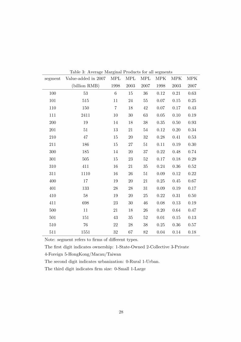
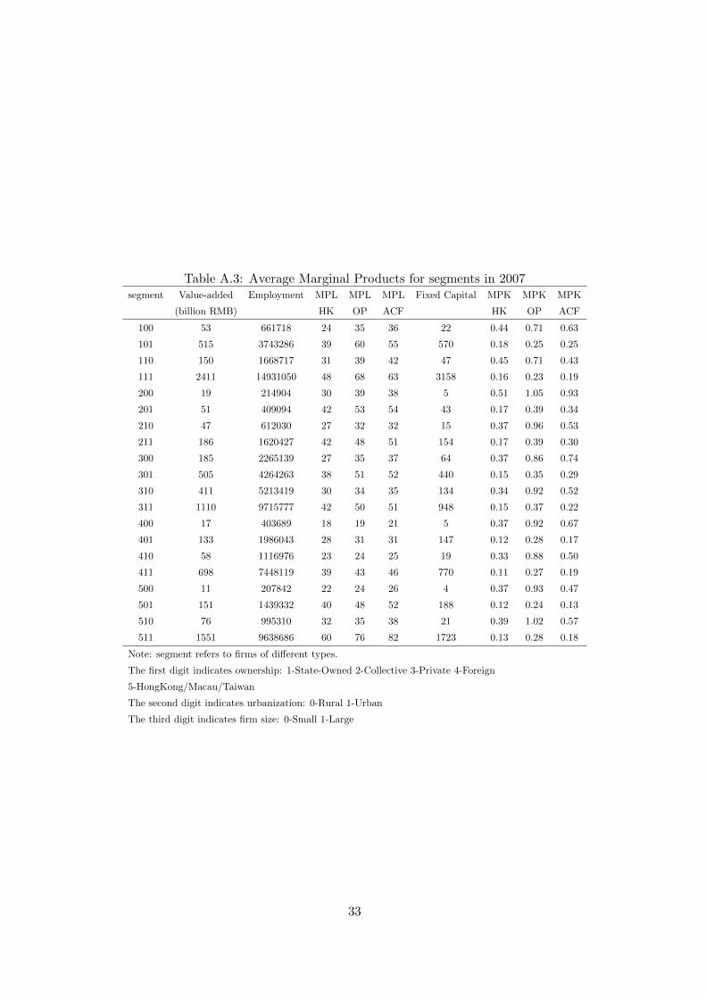
Between-segment capital distortions have been slackening during the economic trans-
formation. Table 3 lists the average marginal products of labour and capital for firm
segments. In 1998 marginal products of capital in state-owned enterprises were approxi-
mately half of the capital productivity in private, collective and foreign companies. Nine
years later state-owned plants have become only 20-40% less efficient in capital than pri-
vate and collective firms and make no clear difference with foreign joint ventures including
those funded from Hong Kong, Macau and Taiwan. Capital in rural regions has 10-30%
18National Bureau of Statistics of China reports that population of migrant labour exceeds 250 million
in 2011.19Beijing, Shanghai, and Guangdong are the representative municipalities/province for Bohai bay eco-
nomic rim in North China, Yangtze river delta in East China and Pearl river delta in South China.20Table A.2 in the appendix reports the average marginal products in 2007 for all the provinces with
different production estimators.
19
higher return than the urban investment for state-owned, collective and private business-
es. Great disparity of capital returns still remains in firm size. Small companies are more
than twice as efficient as big competitors in all five types of ownership. Reversing the
entrenched investment policies that are biased towards large urban SOEs needs to be the
key objective in the reforms of financial sectors. Development of small loan businesses
could offer more means of financing for small private companies in rural regions.
⇒ Insert Table 3 approximately here ⇐
SOEs also catch up with foreign firms in terms of labour productivity and surpass
collective and private companies on average from 1998 to 2007. The difference in marginal
products of labour between urban and rural areas is small. State-owned or foreign firms
have higher labour returns in cities while rural workers are slightly more productive in
collective or private companies. In contrast to the findings regarding capital productivity,
small manufacturers are 20-50% less efficient in labour than the big firms. As also explained
by Qian and Zhu (2013), difficulties in financing force those small private businesses to
employ more workers that substitute for capital and thereby lower the marginal products
of labour.21
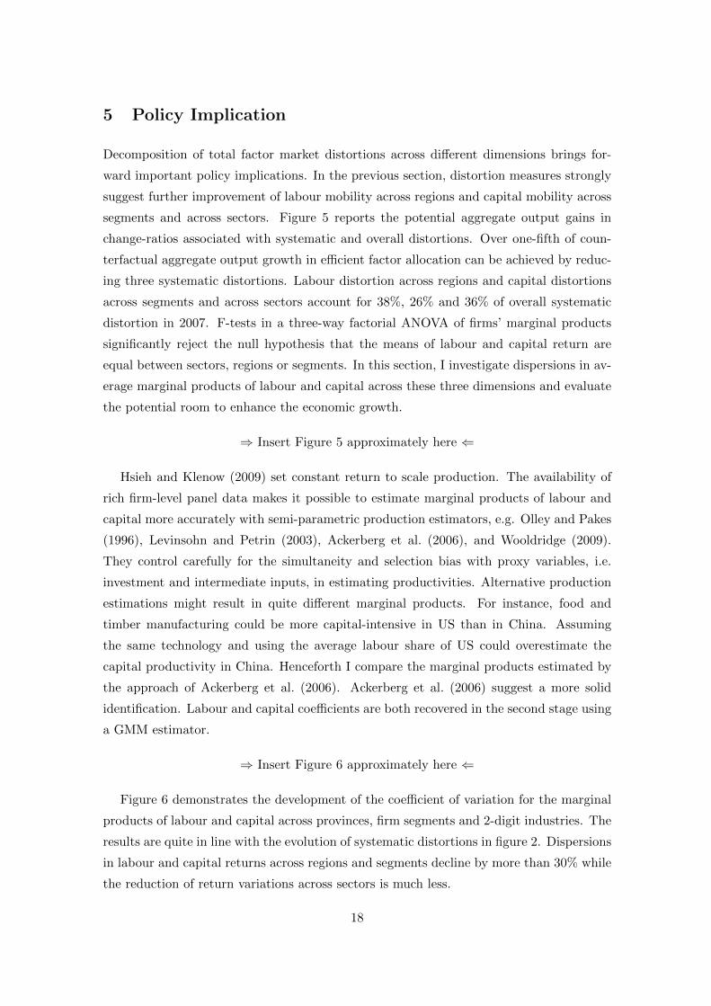
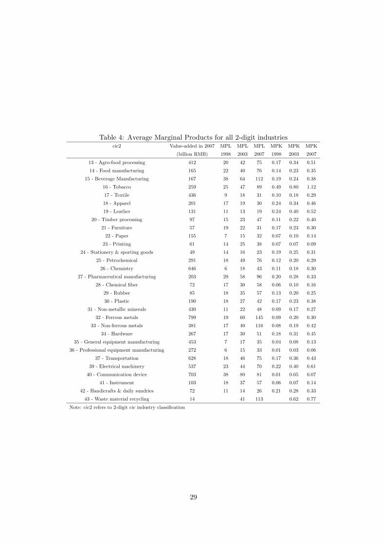
Table 4 lists the average marginal products of labour and capital for all 2-digit indus-
tries. Industries with high capital productivity include tobacco, food processing, textile,
electrical machinery and waste materials recycling. Manufacturing of general and profes-
sional equipment, communication device, instrument, paper and printing have low pro-
ductivity of capital. Among them, communication device production such as television
and computer experienced a rapid capital accumulation of 322% growth for the period
1998-2007 but suffer with one of the lowest marginal products of capital. Over-investment
in those sectors is blamed on the excessive financing support by the state-dominated banks
and local governments. Demand suppressed by the inferior techniques finally results in
the over-capacity in production. This is not the unique case. For instance, steeling and
photovoltaic industries acquired excessive capital from government stimulus in the global
economic turmoil and have confronted serious capacity plethora when demand restores
or faces new trade barriers.22 Recently, the old television lesson repeats for LED. Large
amount of government-backed loans are invested in the capacity of outdating techniques
while international competitors such as Samsung and Sony start mass production of tele-
visions with a new generation of techniques. Governments should definitely give up these
21Table A.3 in the appendix reports the average marginal products in 2007 for all the segments with
different production estimators.22US has been imposing 31%-250% anti-dumping duties on photovoltaic (PV) from China since May
2012. EU launched Chinese anti-dumping PV investigation in September 2012.
20
inefficient financing support and gradually liberalize banks with autonomous interest rates
on both deposit and credit.
⇒ Insert Table 4 approximately here ⇐
Product per worker also deviates across sectors. This reflects more than the sectoral
differentials in labour quality as the marginal product of labour in the least productive
sectors are less than doubled on average in the decade while labour in the most productive
sectors has become over four times more productive in the same period. However, differ-
ent requirement of labour skills across sectors installs barriers for labour mobility. The
tobacco industry has high marginal products in both capital and labour. Metallurgy and
petrochemical have relatively high labour productivity. Resources moving to those sectors
must also be restrained in the light of negative externalities, i.e. increasing public health
care expenditure, high pollution and energy consumption.23
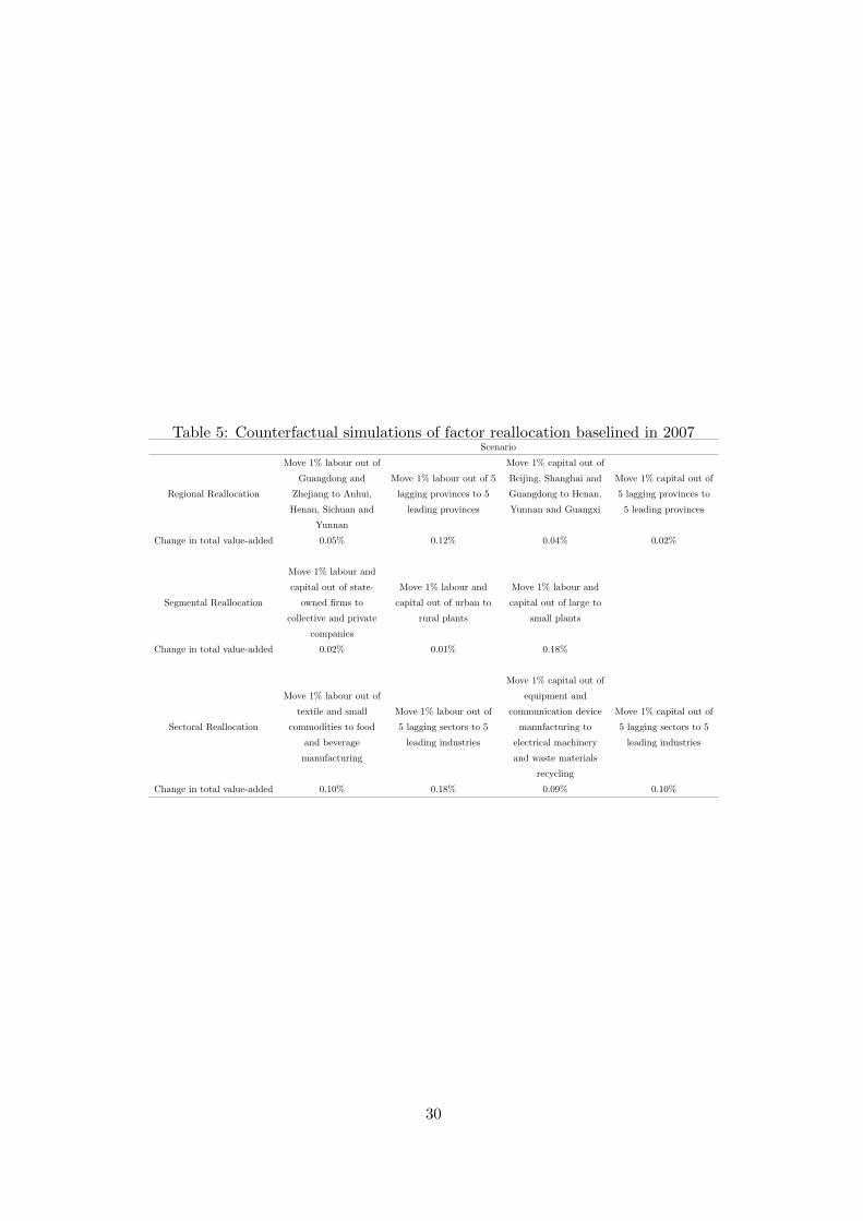
⇒ Insert Table 5 approximately here ⇐
Table 5 reports the potential increase in total manufacturing value-added of the coun-
terfactual factor reallocations. I only estimate the impact of small percentage factor
reallocations as marginal products may stay roughly constant.24 The top panel of Table
5 simulates the regional reallocation baselined in 2007. Moving 1% manufacturing labour
out of Guangdong and Zhejiang to selective Central and Western provinces boosts the
total manufacturing GDP by 0.05%. An inland shift of labour-intensive sectors would
slow down the inefficient coastal labour migration and have positive impacts on local eco-
nomic development. Keeping production within China’s borders also avoids decamping of
international manufacturers and encourages the industrial upgrading in coastal regions. A
better restructuring of 1% labour from 5 lagging provinces to 5 leading provinces provides
a potential output growth of 0.12%. Shifting 1% capital of Beijing, Shanghai and Guang-
dong to Henan, Yunnan and Guangxi improves the capital efficiency and gives rise to a
0.04% growth of GDP in manufacturing. Moving 1% capital out of 5 lagging provinces to
5 leading provinces arouses weaker contribution as the lagging provinces in Northwest and
Northeast possess much less capital in manufacturing than those three capital abundant
provinces.
23Table A.4 in the appendix reports the average marginal products in 2007 for all the sectors with
different production estimators.24For a gross output production function, we also need to consider the differentials in demand elastic-
ities across sectors. The ideal movement would be to attract the resources from less productive inelastic
sectors to more productive elastic sectors. Less productive sectors produce less but the price increase will
compensate as much. Sectors that are more productive can produce more with unchanged prices.
21
The middle panel discloses the impact of segmental reallocations between ownership,
level of urbanization and firm size. Sending 1% of production capacity from state-owned
enterprises to collective and private companies, from urban to rural plants, and from
large to small firms yields gains in aggregate value-added of 0.02%, 0.01% and 0.18%
respectively. Considerable impacts from firm size confirm the importance of developing
small credit markets. Improvement of disparities in ownership and between urban and
rural areas could additionally deliver equally important social consequences since large
inequalities are a potential source of social conflict and instability (Zhang and Tan, 2007).
The bottom panel in Table 5 evaluates four scenarios of sectoral reallocation. Moving
1% labour out of textile and small commodities and distributing proportionally accord-
ing to value-added among food and beverage manufacturing could increase manufacturing
GDP by 0.1%. Compared to the other sectors with high labour productivity such as metal-
lurgy and pharmaceuticals, food and beverage manufacturing have low demand for labour
skills. Reallocating low-skill workforce between those labour-intensive sectors is relatively
easy to realize. Moving 1% labour out of 5 lagging sectors to 5 leading industries increases
more value-added but requires extra social costs to retrain workers. Divesting 1% capital
out of over-invested sectors, i.e. equipment and communication device manufacturing,
to electrical machinery and waste materials recycling increases aggregate value-added by
0.09%. Capital is largely injected into fixed assets and becomes stubborn to shift among
sectors. Electrical machinery and waste materials recycling are likely to share part of the
production techniques, materials and machinery with those inefficient sectors and are able
to absorb some of the over-capacities. Moving 1% capital out of 5 lagging sectors to 5
leading industries is therefore rather theoretical and raises manufacturing GDP by 0.1%.
Divesture of inefficient sectors is however belated effort. Government must reduce its role
in financing manufacturing sectors to fundamentally improve the capital mobility across
sectors.
6 Conclusion
In this paper, I decompose firm-level distortions in China’s manufacturing sectors into
systematic components, i.e. labour distortion across regions, capital distortions across
segments and across sectors, and idiosyncratic residuals. In the framework of Hsieh and
Klenow (2009), an extended model suggests that most of allocative efficiency gains with-
in manufacturing sectors are associated with the reductions of labour distortions across
regions and capital distortions across segments from 1998 to 2007. Improvement of misal-
location across sectors is limited. Rising idiosyncratic distortions after 2002 are responsible
for the setback of total allocative efficiency over time. Systematic distortions across re-
22
gions, segments and sectors are still significant in 2007 and provide great potentials for
economic growth.
Those findings are robust to alternative measurement error corrections, labour hetero-
geneity across firms, and aggressive elasticity of substitution in monopolistic competition.
However, some caveats for the limits of the model must be added. First, existing measure-
ment errors might still overstate the distortions, despite the evidence provided by Hsieh
and Klenow (2009) to reassure that remaining measurement errors in China’s manufac-
turing microdata do not account for big TFP gains. Second, unit elasticity of substitution
across sectors constrains the sectoral reallocation to estimate distortions across sectors,
although it is not rejected in Chinese data. Third, policy distortions and impact of entry
and exit are not separately taken into account.
Counterfactual policy simulations across regions, segments and sectors suggest that
reallocating labour among labour-intensive sectors and transferring those sectors from
coastal regions, i.e. Zhejiang and Guangdong, to selective Central and Western provinces
could achieve modest increases of GDP in manufacturing. In terms of capital reallocation,
the government must reduce its role in financing manufacturing sectors and avoid the
abuse of capital in metropolitan areas. Restructuring the financial system that is biased
towards big state-owned urban firms might result in considerable economic growth, which
gives rise to the urgence of developing small credit markets.
Table 1: Summary statistics on data sample in manufacturing sector
Year Number Value Output Employment Net value of
of firms Added fixed assets
1998 149,692 1.52 5.96 46.32 4.02
1999 147,116 1.71 6.57 47.61 4.26
2000 148,277 1.99 7.55 44.47 4.48
2001 155,409 2.21 8.52 44.11 4.50
2002 166,868 2.66 10.36 46.17 4.69
2003 181,186 3.41 13.20 48.84 5.04
2004 256,026 4.40 17.05 56.61 5.89
2005 251,499 5.41 20.41 59.35 6.58
2006 279,282 6.74 25.23 63.47 7.44
2007 313,048 8.34 31.55 68.56 8.48
Notes: The unit is trillion RMB for the values and millions of
workers for employment
23
Figure 1: Input allocation by firm type
(a) Employment by region (b) Fixed capital by ownership
(c) Fixed capital by level of urbanization and
firm size
(d) Fixed capital by industries
Figure 2: Decomposition of distortions over time
(a) Aggregate distortions
(b) Decomposition of labour distortion (c) Decomposition of capital distortion
24
Figure 3: Robustness checks of systematic distortions within sectors
(a) Between-region labour distortion within
sectors
(b) Between-segment capital distortion within
sectors
Figure 4: Distortion decomposition of manufacturing in EU-15
(a) Decomposition of labour distortion in EU-
15
(b) Decomposition of capital distortion in EU-
15
Figure 5: Growth potentials in aggregate output
25
Figure 6: Coefficient of variation for MRPL and MRPK across regions, segments and
sectors
(a) Coefficient of variation across regions (b) Coefficient of variation across segments
(c) Coefficient of variation across sectors
26
Table 2: Average Marginal Products for all provinces
province Value-added in 2007 MPL MPL MPL MPK MPK MPK
(billion RMB) 1998 2003 2007 1998 2003 2007
11 - Beijing 151 19 48 69 0.03 0.08 0.10
12 - Tianjin 202 13 30 71 0.01 0.12 0.23
13 - Hebei 326 11 27 56 0.10 0.19 0.28
14 - Shanxi 125 8 15 36 0.05 0.09 0.16
15 - Inner Mongolia 129 8 28 82 0.05 0.11 0.24
21 - Liaoning 403 8 26 66 0.05 0.11 0.22
22 - Jiling 143 12 39 80 0.07 0.18 0.25
23 - Heilongjiang 75 8 22 41 0.04 0.09 0.14
31 - Shanghai 462 23 57 79 0.06 0.12 0.17
32 - Jiangsu 1073 14 35 60 0.07 0.14 0.19
33 - Zhejiang 614 15 26 36 0.07 0.14 0.17
34 - Anhui 183 10 26 58 0.10 0.18 0.26
35 - Fujian 284 18 27 38 0.12 0.14 0.27
36 - Jiangxi 137 8 22 56 0.06 0.16 0.31
37 - Shandong 1125 12 31 67 0.12 0.21 0.29
41 - Henan 460 9 20 64 0.11 0.19 0.37
42 - Hubei 236 14 28 57 0.09 0.10 0.20
43 - Hunan 215 10 25 55 0.07 0.13 0.27
44 - Guangdong 1087 20 34 43 0.08 0.12 0.18
45 - Guangxi 111 10 22 57 0.07 0.11 0.35
46 - Hainan 20 22 43 119 0.08 0.13 0.21
50 - Chongqiang 103 8 25 50 0.02 0.11 0.19
51 - Sichuan 283 10 26 57 0.05 0.13 0.23
52 - Guizhou 51 6 15 38 0.11 0.16 0.27
53 - Yunnan 110 21 41 64 0.20 0.25 0.36
54 - Tibet 1 13 26 60 0.09 0.16 0.19
61 - Shaanxi 111 8 19 53 0.03 0.05 0.16
62 - Gansu 55 8 22 45 0.03 0.08 0.19
63 - Qinghai 15 9 22 47 0.05 0.11 0.20
64 - Ningxia 19 8 21 49 0.07 0.11 0.20
65 - Xinjiang 30 8 27 35 0.06 0.10 0.15
Note: province refers to 2-digit national region classification
27
Table 3: Average Marginal Products for all segments
segment Value-added in 2007 MPL MPL MPL MPK MPK MPK
(billion RMB) 1998 2003 2007 1998 2003 2007
100 53 6 15 36 0.12 0.21 0.63
101 515 11 24 55 0.07 0.15 0.25
110 150 7 18 42 0.07 0.17 0.43
111 2411 10 30 63 0.05 0.10 0.19
200 19 14 18 38 0.35 0.50 0.93
201 51 13 21 54 0.12 0.20 0.34
210 47 15 20 32 0.28 0.41 0.53
211 186 15 27 51 0.11 0.19 0.30
300 185 14 20 37 0.22 0.48 0.74
301 505 15 23 52 0.17 0.18 0.29
310 411 16 21 35 0.24 0.36 0.52
311 1110 16 26 51 0.09 0.12 0.22
400 17 19 20 21 0.25 0.45 0.67
401 133 28 28 31 0.09 0.19 0.17
410 58 19 20 25 0.22 0.31 0.50
411 698 23 30 46 0.08 0.13 0.19
500 11 21 18 26 0.20 0.64 0.47
501 151 43 35 52 0.01 0.15 0.13
510 76 22 28 38 0.25 0.36 0.57
511 1551 32 67 82 0.04 0.14 0.18
Note: segment refers to firms of different types.
The first digit indicates ownership: 1-State-Owned 2-Collective 3-Private
4-Foreign 5-HongKong/Macau/Taiwan
The second digit indicates urbanization: 0-Rural 1-Urban.
The third digit indicates firm size: 0-Small 1-Large
28
Table 4: Average Marginal Products for all 2-digit industriescic2 Value-added in 2007 MPL MPL MPL MPK MPK MPK