357

FACTORIAL LINEAR MODELANALYSIS
BY
Christopher J. Brien
B. Sc. Agric. (Sydney)
M. Agr. Sc. (Adelaide)
Thesis submitted for the Degree of
Doctor of Philosophy
in the Department of Plant Science,
The University of Adelaide.
February 1992

ii
Contents
List of tables vi
List of �gures x
Summary xii
Signed statement xiii
Acknowledgements xiv
1 Factorial linear model analysis: a review 11.1 Introduction . . . . . . . . . . . . . . . . . . . . . . . . . . . . . . . . 11.2 Existing analyses . . . . . . . . . . . . . . . . . . . . . . . . . . . . . 2
1.2.1 Randomization models . . . . . . . . . . . . . . . . . . . . . . 31.2.1.1 Neyman/Wilk/Kempthorne formulation . . . . . . . 31.2.1.2 Nelder/White/Bailey formulation . . . . . . . . . . . 61.2.1.3 Discussion . . . . . . . . . . . . . . . . . . . . . . . . 11
1.2.2 General linear models . . . . . . . . . . . . . . . . . . . . . . . 121.2.2.1 Fixed e�ects linear models . . . . . . . . . . . . . . . 131.2.2.2 Mixed linear models . . . . . . . . . . . . . . . . . . 181.2.2.3 Fixed versus random factors . . . . . . . . . . . . . . 27
1.3 Randomization versus general linear models . . . . . . . . . . . . . . 281.4 Unresolved problems . . . . . . . . . . . . . . . . . . . . . . . . . . . 31
2 The elements of the approach to linear model analysis 322.1 Introduction . . . . . . . . . . . . . . . . . . . . . . . . . . . . . . . . 322.2 The elements of the approach . . . . . . . . . . . . . . . . . . . . . . 34
2.2.1 Observational unit and factors . . . . . . . . . . . . . . . . . . 352.2.2 Tiers . . . . . . . . . . . . . . . . . . . . . . . . . . . . . . . . 362.2.3 Expectation and variation factors . . . . . . . . . . . . . . . . 382.2.4 Structure set . . . . . . . . . . . . . . . . . . . . . . . . . . . 392.2.5 Analysis of variance table . . . . . . . . . . . . . . . . . . . . 44

Contents iii
2.2.6 Expectation and variation models . . . . . . . . . . . . . . . . 532.2.6.1 Generating the maximal expectation and variationmodels
532.2.6.2 Generating the lattices of expectation and variation
models . . . . . . . . . . . . . . . . . . . . . . . . . . 562.2.7 Expected mean squares . . . . . . . . . . . . . . . . . . . . . . 612.2.8 Model �tting/testing . . . . . . . . . . . . . . . . . . . . . . . 63
2.2.8.1 Selecting the variation model . . . . . . . . . . . . . 642.2.8.2 Selecting the expectation model . . . . . . . . . . . . 66
3 Analysis of variance quantities 683.1 Introduction . . . . . . . . . . . . . . . . . . . . . . . . . . . . . . . . 683.2 The algebraic analysis of a single structure . . . . . . . . . . . . . . . 743.3 Derivation of rules for analysis of variance quantities . . . . . . . . . 95
3.3.1 Analysis of variance for the study . . . . . . . . . . . . . . . . 953.3.1.1 Recursive algorithm for the analysis of variance . . . 108
3.3.2 Linear models for the study . . . . . . . . . . . . . . . . . . . 1123.3.3 Expectation and distribution of mean squares for the study . . 117
3.4 Discussion . . . . . . . . . . . . . . . . . . . . . . . . . . . . . . . . . 124
4 Analysis of two-tiered experiments 1274.1 Introduction . . . . . . . . . . . . . . . . . . . . . . . . . . . . . . . . 1274.2 Application of the approach to two-tiered experiments . . . . . . . . . 128
4.2.1 A two-tiered sensory experiment . . . . . . . . . . . . . . . . . 1284.2.1.1 Split-plot analysis of a two-tiered sensory experiment 134
4.2.2 Nonorthogonal two-factor experiment . . . . . . . . . . . . . . 1354.2.3 Nested treatments . . . . . . . . . . . . . . . . . . . . . . . . 142
4.2.3.1 Treated-versus-control . . . . . . . . . . . . . . . . . 1424.2.3.2 Sprayer experiment . . . . . . . . . . . . . . . . . . 147
4.3 Clarifying the analysis of complex two-tiered experiments . . . . . . . 1524.3.1 Split-plot designs . . . . . . . . . . . . . . . . . . . . . . . . . 1534.3.2 Experiments with two or more classes of replication factors . . 156
4.3.2.1 Single class in bottom tier . . . . . . . . . . . . . . . 1574.3.2.2 Two or more classes in bottom tier, factors random-
ized to only one . . . . . . . . . . . . . . . . . . . . 1604.3.2.3 Factors randomized to two or more classes in bottom
tier, no carry-over . . . . . . . . . . . . . . . . . . . 1704.3.2.4 Factors randomized to two or more classes in bottom
tier, carry-over . . . . . . . . . . . . . . . . . . . . . 172

Contents iv
5 Analysis of three-tiered experiments 1785.1 Introduction . . . . . . . . . . . . . . . . . . . . . . . . . . . . . . . . 1785.2 Two-phase experiments . . . . . . . . . . . . . . . . . . . . . . . . . . 179
5.2.1 A sensory experiment . . . . . . . . . . . . . . . . . . . . . . . 1795.2.2 McIntyre's experiment . . . . . . . . . . . . . . . . . . . . . . 1845.2.3 Taste-testing experiment from Wood, Williams and Speed (1988)1925.2.4 Three structures required . . . . . . . . . . . . . . . . . . . . 204
5.3 Superimposed experiments . . . . . . . . . . . . . . . . . . . . . . . . 2135.3.1 Conversion of a completely randomized design . . . . . . . . . 2135.3.2 Conversion of a randomized complete block design . . . . . . . 2145.3.3 Conversion of Latin square designs . . . . . . . . . . . . . . . 216
5.4 Single-stage experiments . . . . . . . . . . . . . . . . . . . . . . . . . 2185.4.1 Plant experiments . . . . . . . . . . . . . . . . . . . . . . . . . 2195.4.2 Animal experiments . . . . . . . . . . . . . . . . . . . . . . . 2215.4.3 Split plots in a row-and-column design . . . . . . . . . . . . . 225
6 Problems resolved by the present approach 2296.1 Extent of the method . . . . . . . . . . . . . . . . . . . . . . . . . . . 2296.2 The basis for inference . . . . . . . . . . . . . . . . . . . . . . . . . . 2316.3 Factor categorizations . . . . . . . . . . . . . . . . . . . . . . . . . . 2356.4 Model composition and the role of parameter constraints . . . . . . . 2396.5 Appropriate mean square comparisons . . . . . . . . . . . . . . . . . 2416.6 Form of the analysis of variance table . . . . . . . . . . . . . . . . . . 243
6.6.1 Analyses re ecting the randomization . . . . . . . . . . . . . . 2446.6.2 Types of variability . . . . . . . . . . . . . . . . . . . . . . . . 2526.6.3 Highlighting inadequate replication . . . . . . . . . . . . . . . 257
6.7 Partition of the Total sum of squares . . . . . . . . . . . . . . . . . . 260
7 Conclusions 263
A Data for examples 266A.1 Data for two-tiered sensory experiment of section 4.2.1 . . . . . . . . 267A.2 Data for the sprayer experiment of section 4.2.3.2 . . . . . . . . . . . 268A.3 Data for repetitions in time experiment of section 4.3.2.2 . . . . . . . 269A.4 Data for the three-tiered sensory experiment of section 5.2.4 . . . . . 270
B Reprint of Brien (1983) 275
C Reprint of Brien (1989) 280
Glossary 296
Notation 315

Contents v
Bibliography 322

vi
List of tables
1.1 Analysis of variance table with expected mean squares using the Ney-man/Wilk/Kempthorne formulation. . . . . . . . . . . . . . . . . . . 7
1.2 Analysis of variance table with expected mean squares using the Nelderformulation. . . . . . . . . . . . . . . . . . . . . . . . . . . . . . . . 11
2.1 Rules for deriving the analysis of variance table from the structure set 452.2 Steps for computing the degrees of freedom for the analysis of variance 482.3 Steps for computing the sums of squares for the analysis of variance in
orthogonal studies . . . . . . . . . . . . . . . . . . . . . . . . . . . . . 492.4 Analysis of variance table for a split-plot experiment with main plots
in a Latin square design . . . . . . . . . . . . . . . . . . . . . . . . . 522.5 Steps for determining the maximal expectation and variation models 542.6 Generating the expectation and variation lattices of models . . . . . . 572.7 Interpretation of variation models for a split-plot experiment with main
plots in a Latin square design . . . . . . . . . . . . . . . . . . . . . . 602.8 Steps for determining the expected mean squares for the maximal ex-
pectation and variation models . . . . . . . . . . . . . . . . . . . . . 612.9 Analysis of variance table for a split-plot experiment with main plots
in a Latin square design. . . . . . . . . . . . . . . . . . . . . . . . . . 622.10 Analysis of variance table for a split-plot experiment with main plots
in a Latin square design. . . . . . . . . . . . . . . . . . . . . . . . . . 652.11 Estimates of expectation parameters for a split-plot experiment with
main plots in a Latin square design. . . . . . . . . . . . . . . . . . . . 67
3.1 Analysis of variance table for a simple lattice experiment . . . . . . . 733.2 Direct product expressions for the incidence, summation and idempo-
tent matrices for (R �C)=S=U . . . . . . . . . . . . . . . . . . . . . 843.3 Analysis of variance table, including projection operators, for a split-
plot experiment . . . . . . . . . . . . . . . . . . . . . . . . . . . . . . 1063.4 Analysis of variance table, including projection operators, for a simple
lattice experiment . . . . . . . . . . . . . . . . . . . . . . . . . . . . . 107

List of tables vii
3.5 Analysis of variance table, including projection operators, for a split-plot experiment . . . . . . . . . . . . . . . . . . . . . . . . . . . . . . 124
3.6 Analysis of variance table, including projection operators, for a simplelattice experiment . . . . . . . . . . . . . . . . . . . . . . . . . . . . . 125
4.1 Analysis of variance table for a two-tiered sensory experiment. . . . . 1304.2 Split-plot analysis of variance table for a two-tiered sensory experiment 1364.3 The structure set and analysis of variance for a nonorthogonal two-
factor completely randomized design . . . . . . . . . . . . . . . . . . 1384.4 Contribution to the expected mean squares from the expectation fac-
tors for the two-factor experiment under alternative models . . . . . . 1404.5 Analysis of variance table for the treated-versus-control experiment . 1444.6 Table of means for the treated-versus-control experiment . . . . . . . 1454.7 Table of application rates and factor levels for the sprayer experiment 1484.8 Analysis of variance table for the sprayer experiment . . . . . . . . . 1504.9 Table of means for the sprayer experiment . . . . . . . . . . . . . . . 1514.10 Structure set and analysis of variance table for the standard split-plot
experiment . . . . . . . . . . . . . . . . . . . . . . . . . . . . . . . . . 1544.11 Structure set and analysis of variance table for the standard split-plot
experiment, modi�ed to include the D.Blocks interaction . . . . . . . 1554.12 Yates and Cochran (1938) analysis of variance table for an experiment
involving sites and years . . . . . . . . . . . . . . . . . . . . . . . . . 1584.13 Structure set and analysis of variance table for an experiment involving
sites and years . . . . . . . . . . . . . . . . . . . . . . . . . . . . . . . 1594.14 Analysis of variance table for the split-plot analysis of a repeated mea-
surements experiment involving only repetitions in time . . . . . . . . 1614.15 Structure set and analysis of variance table for a repeated measure-
ments experiment involving only repetitions in time . . . . . . . . . . 1624.16 Structure set and analysis of variance table for an experiment involving
repetitions in time and space . . . . . . . . . . . . . . . . . . . . . . . 1644.17 Experimental layout for a repeated measurements experiment involving
split plots and split blocks (Federer, 1975) . . . . . . . . . . . . . . . 1654.18 Analysis of variance table for a repeated measurements experiment
involving split plots and split blocks . . . . . . . . . . . . . . . . . . . 1674.19 Federer (1975) Analysis of variance table for a repeated measurements
experiment involving split plots and split blocks . . . . . . . . . . . . 1694.20 Analysis of variance table for a repeated measurements experiment with
factors randomized to two classes of replication factors, no carry-overe�ects . . . . . . . . . . . . . . . . . . . . . . . . . . . . . . . . . . . 171
4.21 Analysis of variance table for the change-over experiment from Cochranand Cox (1957, section 4.62a) . . . . . . . . . . . . . . . . . . . . . . 174
4.22 Experimental layout for a change-over experiment with preperiod . . 176

List of tables viii
4.23 Analysis of variance table for the change-over experiment with preperiod177
5.1 Analysis of variance table for a two-phase wine-evaluation experiment 1815.2 Analysis of variance table, including intertier interactions, for a two-
phase wine-evaluation experiment . . . . . . . . . . . . . . . . . . . . 1835.3 Analysis of variance table for McIntyre's two-phase experiment . . . . 1895.4 Scores from the Wood, Williams and Speed (1988) processing experiment1935.5 Analysis of variance table for Wood, Williams and Speed (1988) pro-
cessing experiment . . . . . . . . . . . . . . . . . . . . . . . . . . . . 1965.6 Analysis of variance table for the Wood, Williams and Speed (1988)
storage experiment . . . . . . . . . . . . . . . . . . . . . . . . . . . . 1995.7 Analysis of variance table after that presented by Wood, Williams and
Speed (1988) for a taste-testing experiment . . . . . . . . . . . . . . 2025.8 Assignment of the trellis treatment to the main plots in the �eld phase
of the experiment. . . . . . . . . . . . . . . . . . . . . . . . . . . . . . 2045.9 Assignment of the main plots (Row and Column combinations) from
the �eld experiment to the judges at each sitting in the evaluation phase.2055.10 Analysis of variance table for an experiment requiring three tiers . . . 2095.11 Information summary for an experiment requiring three tiers . . . . . 2105.12 Structure set and analysis of variance table for a superimposed experi-
ment based on a completely randomized design . . . . . . . . . . . . 2145.13 Structure set and analysis of variance table for a superimposed experi-
ment based on a randomized complete block design . . . . . . . . . . 2155.14 Structure set and analysis of variance table for superimposed experi-
ments based on Latin square designs . . . . . . . . . . . . . . . . . . 2175.15 Structure set and analysis of variance table for a three-tiered plant
experiment . . . . . . . . . . . . . . . . . . . . . . . . . . . . . . . . . 2205.16 Structure set and analysis of variance table for a grazing experiment . 2225.17 Structure set and analysis of variance table for the revised grazing
experiment . . . . . . . . . . . . . . . . . . . . . . . . . . . . . . . . . 2245.18 Experimental layout for a split-plot experiment with split plots ar-
ranged in a row-and-column design (Federer, 1975) . . . . . . . . . . 2265.19 Structure set and analysis of variance table for a split-plot experiment
with split plots arranged in a row-and-column design (Federer, 1975) 2275.20 Information summary for a split-plot experiment with split plots ar-
ranged in a row-and-column design (Federer, 1975) . . . . . . . . . . 228
6.1 Analysis of variance for an observational study . . . . . . . . . . . . . 2336.2 Randomized complete block design analysis of variance tables for two
alternative structure sets . . . . . . . . . . . . . . . . . . . . . . . . . 2456.3 Structure sets and models for the three experiments discussed by White
(1975) and a multistage survey . . . . . . . . . . . . . . . . . . . . . 248

List of tables ix
6.4 Analysis of variance tables for the three experiments described byWhite (1975) and a multistage survey . . . . . . . . . . . . . . . . . . 250
6.5 Structure sets and analysis of variance tables for the randomized com-plete block design assuming either a) intertier additivity, b) intertierinteraction, or c) treatment error . . . . . . . . . . . . . . . . . . . . 255
6.6 Structure sets and analysis of variance tables for the randomized com-plete block design assuming both intertier interaction and treatmenterror . . . . . . . . . . . . . . . . . . . . . . . . . . . . . . . . . . . . 256
6.7 Structure set and analysis of variance table for a growth cabinet ex-periment . . . . . . . . . . . . . . . . . . . . . . . . . . . . . . . . . . 258
6.8 Structure sets and analysis of variance tables for Addelman's (1970)experiments . . . . . . . . . . . . . . . . . . . . . . . . . . . . . . . . 259
A.1 Scores for the two-tiered sensory experiment of section 4.2.1 . . . . . 267A.2 Lightness readings and assignment of Pressure-Speed combinations for
the sprayer experiment of section 4.2.3.2 . . . . . . . . . . . . . . . . 268A.3 Yields and assignment of Clones for the repetitions in time experiment
of section 4.3.2.2 . . . . . . . . . . . . . . . . . . . . . . . . . . . . . 269A.4 Scores and assignment of factors for Occasion 1, Judges 1{3 from the
experiment of section 5.2.4 . . . . . . . . . . . . . . . . . . . . . . . . 271A.5 Scores and assignment of factors for Occasion 1, Judges 4{6 from the
experiment of section 5.2.4 . . . . . . . . . . . . . . . . . . . . . . . . 272A.6 Scores and assignment of factors for Occasion 2, Judges 1{3 from the
experiment of section 5.2.4 . . . . . . . . . . . . . . . . . . . . . . . . 273A.7 Scores and assignment of factors for Occasion 2, Judges 4{6 from the
experiment of section 5.2.4 . . . . . . . . . . . . . . . . . . . . . . . . 274

x
List of �gures
2.1 Field layout and yields of oats for split-plot experiment . . . . . . . . 352.2 Hasse Diagram of term marginalities for a split-plot experiment with
degrees of freedom . . . . . . . . . . . . . . . . . . . . . . . . . . . . 502.3 Hasse diagram of term marginalities for a split-plot experiment with
e�ects vectors . . . . . . . . . . . . . . . . . . . . . . . . . . . . . . . 512.4 Lattices of models for a split-plot experiment in which the main plots
are arranged in a Latin square design . . . . . . . . . . . . . . . . . . 58
3.1 Field layout and yields for a simple lattice experiment . . . . . . . . . 703.2 Hasse diagram of term marginalities for a simple lattice experiment . 713.3 Decomposition tree for a simple lattice experiment . . . . . . . . . . . 723.4 Hasse diagram of term marginalities, including fTiws, for the (R �
C)=S=U example . . . . . . . . . . . . . . . . . . . . . . . . . . . . . 893.5 Decomposition tree for a four-tiered experiment with 5,8,5, and 3 terms
arising from each of structures 1{4, respectively . . . . . . . . . . . . 973.6 Decomposition tree for a split-plot experiment . . . . . . . . . . . . . 105
4.1 Hasse diagram of term marginalities for a two-tiered sensory experiment1294.2 Sublattices of variation models for second and third order model selec-
tion in a sensory experiment . . . . . . . . . . . . . . . . . . . . . . . 1334.3 Hasse Diagram of term marginalities for a nonorthogonal two-factor
completely randomized design . . . . . . . . . . . . . . . . . . . . . . 1374.4 Lattices of models for the two-factor completely randomized design . 1394.5 Strategy for expectation model selection for a nonorthogonal two-factor
completely randomized design . . . . . . . . . . . . . . . . . . . . . . 1414.6 Hasse diagram of term marginalities for the treated-versus-control ex-
periment . . . . . . . . . . . . . . . . . . . . . . . . . . . . . . . . . . 1434.7 Lattices of models for the treated-versus-control experiment . . . . . 1464.8 Hasse diagram of term marginalities for the sprayer experiment . . . 149
5.1 Hasse diagram of term marginalities for a sensory experiment . . . . 1805.2 Minimal sweep sequence for a two-phase sensory experiment . . . . . 182

List of figures xi
5.3 Layout for the �rst phase of McIntyre's (1955) experiment . . . . . . 1855.4 Layout for the second phase of McIntyre's (1955) experiment . . . . . 1865.5 Hasse diagram of term marginalities for McIntyre's experiment . . . . 1885.6 Minimal sweep sequence for McIntyre's two-phase experiment . . . . 1915.7 Hasse diagram of term marginalities for the Wood, Williams and Speed
(1988) processing experiment . . . . . . . . . . . . . . . . . . . . . . 1955.8 Minimal sweep sequence for Wood, Williams and Speed (1988) process-
ing experiment . . . . . . . . . . . . . . . . . . . . . . . . . . . . . . 1975.9 Minimal sweep sequence for the Wood, Williams and Speed (1988)
storage experiment . . . . . . . . . . . . . . . . . . . . . . . . . . . . 2005.10 Hasse diagram of term marginalities for an experiment requiring three
tiers . . . . . . . . . . . . . . . . . . . . . . . . . . . . . . . . . . . . 2085.11 Minimal sweep sequence for an experiment requiring three tiers . . . 212

xii
Summary
This thesis develops a general strategy for factorial linear model analysis for experi-
mental and observational studies. It satisfactorily deals with a number of issues that
have previously caused problems in such analyses. The strategy developed here is an
iterative, four-stage, model comparison procedure as described in Brien (1989); it is
a generalization of the approach of Nelder (1965a,b).
The approach is applicable to studies characterized as being structure-balanced,
multitiered and based on Tjur structures unless the structure involves variation fac-
tors when it must be a regular Tjur structure. It covers a wide range of experiments
including multiple-error, change-over, two-phase, superimposed and unbalanced ex-
periments. Examples illustrating this are presented. Inference from the approach is
based on linear expectation and variation models and employs an analysis of variance.
The sources included in the analysis of variance table is based on the division of the
factors, on the basis of the randomization employed in the study, into sets called tiers.
The factors are also subdivided into expectation factors and variation factors. From
this subdivision models appropriate to the study can be formulated and the expected
mean squares based on these models obtained. The terms in the expectation model
may be nonorthogonal and the terms in the variation model may exhibit a certain
kind of nonorthogonal variation structure. Rules are derived for obtaining the sums
of squares, degrees of freedom and expected mean squares for the class of studies
covered.
The models used in the approach make it clear that the expected mean squares
depend on the subdivision into expectation and variation factors. The approach
clari�es the appropriate mean square comparisons for model selection. The analysis
of variance table produced with the approach has the advantage that it will re ect
all the relevant physical features of the study. A consequence of this is that studies,
in which the randomization is such that their confounding patterns di�er, will have
di�erent analysis of variance tables.

xiii
Signed statement
This thesis contains no material which has been accepted for the award of any other
degree or diploma in any university and, to the best of my knowledge and belief, the
thesis contains no material previously published or written by another person, except
where due reference is made in the text of the thesis. The material in chapters 2 and
6, except sections 6.6 and 6.7, is a revised version of that which I have previously
published in Brien (1983) and Brien (1989); copies of these two papers are contained
in appendices B and C. The material in section 5.2.4 and some of that in section 6.7 is
the subject of an unpublished manuscript by Brien and Payne (1989). The analysis for
change-over experiments presented in section 4.3.2.4 was originally developed jointly
by Mr W B Hall and the author; my contribution to the joint work is detailed in the
text.
I consent to the thesis being made available for photocopying and loan if accepted
for the award of the degree.
C.J. Brien

xiv
Acknowledgements
I am greatly appreciative of the considerable support given to me by Mr W B Hall,
Dr O Mayo, Mr RW Payne, Dr D J Street and Dr W N Venables during the conduct of
the research reported herein. I am indebted to Prof. A T James for an appreciation of
the algebraic approach to the analysis of variance. I am also grateful to Mr K Cellier,
Professor Sir David Cox, Mr R R Lamacraft and the many referees of draft versions of
papers reporting this work for helpful comments. Also, I am indebted to Mr A J Ewart
for the wine-tasting data which are analysed in section 4.2.1 and which he collected
as part of research funded by the South Australian State Government Wine Research
Grant. In addition, I wish to express my thanks to Dr C Latz for the subjects-with-
repetitions-in-time experiment discussed in section 4.3.2.3.
The work in this thesis, being a part-time activity, has been carried out over a long
period of time. Once again Ellen, James and Melissa have had to su�er the trials,
tribulations and joys of living with a person undertaking such a task. Margaret has
also provided support essential to its achievement. Thank you all.

1
Chapter 1
Factorial linear model analysis: a
review
1.1 Introduction
This thesis is concerned with factorial linear model analysis such as is associated
with the statistical analysis of designed experiments and surveys. That is, it deals
with models in which the independent-variables (X) matrix involves only indicator
variables derived from qualitative or quantitative factors or combinations of such
factors. Thus, multiple regression models and analysis of covariance models, in which
the observed values of the variables are placed in the independent-variable matrix,
are excluded from consideration. However, as in the latter situations, the �tting of
factorial linear models is achieved using least squares.
In this chapter, the literature on factorial linear model analysis published up until
approximately the end of 1984 is reviewed. The review will be conducted by consid-
ering the following classes of models in turn:
1) Randomization models
Linear models in which the stochastic elements are provided by the physical act
of randomization:
1.1 Neyman/Wilk/Kempthorne formulation | linear models with stochastic

1.2 Existing analyses 2
indicator variables whose properties are based on randomization;
1.2 Nelder/White/Bailey formulation | covariances derived under randomiza-
tion and linear contrasts speci�ed for treatment comparisons;
2) General linear models
Linear models for the expectation and variation of the response are speci�ed:
2.1 Fixed e�ects linear models | linear expectation model and variance known
up to a scale factor;
2.2 Mixed linear models | linear expectation and variation model.
1.2 Existing analyses
Central to linear model analysis is the analysis of variance table that is used to
summarize the analysis. As Kempthorne (1975a, 1976b) suggests, the analysis of
variance can be formulated as an orthogonal decomposition of the data vector such
that the Total variance is partitioned into components attributable to identi�able
causes. That is, an analysis of variance can be obtained from a linear model whose
terms have no stochastic properties. Indeed, the analysis of variance can be derived
without reference to a model at all; James (1957) describes the derivation of the
analysis based on relationship matrices which form an algebra. The work of Nelder
(1965a,b) can also be viewed in these terms in that his complete set of binary matrices
corresponds to the mutually orthogonal idempotents that generate the ideals of this
algebra.
However, in order to interpret the results of an analysis one needs to ascribe stochas-
tic properties to at least some of the terms in the model. That is, the e�ects for some
terms must be able to be regarded as random variables with a �nite variance. Two
alternative bases for doing this in experiments are the randomization employed in the
experiment and hypothesis.

1.2.1 Randomization models 3
1.2.1 Randomization models
The randomization argument as a basis for statistical inference was �rst propounded
by Fisher (1935b, 1966) when he developed the randomization test as a means of test-
ing hypotheses without making the assumption of normality. However, Sche��e (1959)
cites Neyman (1923) as having formulated randomization models for the completely
randomized design. Also, Neyman, Iwaskiewicz and Kolodzieczyk (1935) formulated
such models for the randomized complete block design.
Since then randomization models of two basic kinds have been developed as a basis
for inference in designed experiments. The models of the �rst kind were developed
directly from Neyman et al.'s randomization models by Wilk, Kempthorne, Zyskind
and White of the Iowa school and by Ogawa and others. Models of the second kind
were developed by Nelder (1965a,b) with White (1975) and Bailey (1981) outlining
related approaches. This latter kind of model is based on the identi�cation of `block'
and `treatment' factors and on derivation of the associated null randomization distri-
bution.
1.2.1.1 Neyman/Wilk/Kempthorne formulation
As mentioned above, Sche��e (1959) cites Neyman (1923) as having used randomiza-
tion models for the completely randomized design. However, the �rst widely available
usage was by Neyman et al. (1935) in considering hypotheses about treatment di�er-
ences for randomized complete block and Latin square experiments; they introduced
models for the true yield and considered their properties under randomization. Eden
and Yates (1933), Welch (1937), Pitman (1938) and McCarthy (1939) used these
concepts but mainly with reference to signi�cance tests for the Latin square and ran-
domized complete block experiments. Kempthorne (1952) formulated models for a
wide range of experiments incorporating design random variables that take only the
values 0 or 1 and whose stochastic properties are directly based on the randomization
employed in the experiment.
Wilk (1955) used a randomization model for the generalized randomized complete
block design (each treatment replicated r times in each block) to investigate the in-

1.2.1 Randomization models 4
ferential properties of randomization models for this design. Wilk and Kempthorne
(1955, 1956) did this for factorial experiments. Wilk and Kempthorne (1955) in-
corporated the e�ect of complete/incomplete sampling into the models; Wilk and
Kempthorne (1956) introduced the idea of expressing the expected mean squares in
terms of �s, the estimable quantities in the analysis. Wilk and Kempthorne (1957)
carried out the same exercise for the Latin square and corrected the results of Neyman
et al. (1935) on the e�ect of unit-treatment nonadditivity.
Zyskind (1962a) extended the results of Wilk and Kempthorne to regular structures
in which, for every term in the structure, the replication of the levels combinations of
that term are equal. Rao (1959) and Zyskind (1963) applied randomization models
to the balanced incomplete block design, although Rao did not incorporate com-
plete/incomplete sampling considerations. Ogawa has also investigated the inferences
under randomization models which are Neyman randomization models, but with the
addition of unit-treatment additivity assumptions (Ogawa, 1980).
The approach of these authors will be illustrated using the work of Wilk and
Kempthorne (1955, 1956) and Zyskind (1962a) since it represents the most general
treatment, the other authors cited above having considered special cases. To illus-
trate the approach we consider the analysis of the randomized complete block design.
Suppose there are B blocks, P plots per block and T treatments available in total and
that b blocks, p (= t) plots per block and t treatments are selected for observation.
Let
Yijk (i = 1; 2; : : : ; B; j = 1; 2; : : : ; P ; k = 1; 2; : : : ; T )
be the true response of the jth plot in the ith block when it receives the kth treat-
ment. Then the population identity, which gives the sum of a number of population
components that is identically equal to the true response, for this design would be as
follows:
Yijk = Y ::: + (Y i:: � Y :::) + (Y ij: � Y i::) + (Y ::k � Y :::)
+ (Y i:k � Y i:: � Y ::k + Y :::) + (Yijk � Y ij: � Y i:k + Y i::)
= �+ �i + �ij + �k + (��)ik + (��)ijk

1.2.1 Randomization models 5
where
the dot subscript denotes summation over that subscript.
De�ne population components of variation for each term in this model. That is,
�2, �2�, �2�, �
2� , �
2�� and �
2�� with, for example,
�2� =BXi=1
(Y i:: � Y :::)2 / (B � 1)
These components of variation are merely measures of dispersion for the population
quantities on which they are de�ned. Wilk and Kempthorne (1956, 1957) point out
that they are not to be confused with components of variance, the latter being the
variances of random variables.
Now only bt values, of the BPT in the population, are observed. Let
yi?k? (i? = 1; 2; : : : ; b; k? = 1; 2; : : : ; t)
be the observation for the k?th treatment in the i?th block. Then the statistical
model, that is, the model for the observations, is:
yi?k? = �+BXi=1
Si?
i �i +TXk=1
Sk?
k �k +BXi=1
TXk=1
Si?
i Sk?
k (��)ik
+pX
j?=1
Dk?
i?j?
BXi=1
PXj=1
Si?
i Si?j?
i?j �ij
+pX
j?=1
Dk?
i?j?
BXi=1
PXj=1
TXk=1
Si?
i Si?j?
i?j Sk?
k (��)ijk
where
Si?
i =
8>>>><>>>>:1 if the i?th selected block is the ith block in the popu-
lation,
0 otherwise
Sk?
k =
8>>>><>>>>:1 if the k?th selected treatment is the kth treatment in
the population,
0 otherwise

1.2.1 Randomization models 6
Si?j?
i?j =
8>>>>>>><>>>>>>>:
1 if the j?th selected plot in the i? selected block is the
jth plot in the population of plots in the i?th selected
block,
0 otherwise
Dk?
i?j? =
8>>>><>>>>:1 if the k?th selected treatment is applied to the j?th
selected plot in the i?th selected block,
0 otherwise
The Si?
i , Sk?
k and Si?j?
i?j are termed selection variables in that the values they take
re ect the population selection, whereas Dk?
i?j? is a design variable in that the values
it takes re ect the application of treatments to units (Wilk and Kempthorne, 1955).
Their distributional properties can be established by considering the probabilities with
which they take the values 0 and 1; for example,
EhSi
?
i
i= E
��Si
?
i
�2�=
1
B; E
�Si
?
i Si?0
i0
�=
1
B(B � 1)for i 6= i0; i? 6= i?
0
:
It can be shown that these variables are all groupwise independent.
Corresponding to this model is an analysis of variance based on the following sample
identity:
yi?k? = y:: + (yi?: � y::) + (y:k? � y::) + (yi?k? � yi?: � y:k? + y::):
By making use of the properties of the random variables in the statistical model
the expected mean squares for the analysis of variance can be obtained and are as
given in table 1.1 (Zyskind, 1962a).
1.2.1.2 Nelder/White/Bailey formulation
The Nelder (1965a,b) formulation is based on the null randomization distribution and
the division of the factors in an experiment into `block' and `treatment' factors. White
(1975) and Bailey (1981) outline a slightly di�erent approach from that of Nelder
(1965a,b) but one which achieves the same results; White (1975) di�ers from Bailey

1.2.1 Randomization models 7
Table 1.1: Analysis of variance table with expected mean squares using
the Neyman/Wilk/Kempthorne formulation.
SOURCE DF EXPECTED MEAN SQUARESy
Blocks b� 1 ��� + �� + ��� + t��
Treatments t� 1 ��� + �� + ��� + b��
Residual (b� 1)(t� 1) ��� + �� + ���
yThe \cap" sigmas, �s, are the following functions of the population components of variation, �2s:
��� = �2�� ;
�� = �2� �1
T�2�� ;
��� = �2�� �1
P�2�� ;
�� = �2� �1
P�2� �
1
T�2�� +
1
P
1
T�2�� ; and
�� = �2� �1
B�2�� :
(1981) and Nelder (1965a,b) in including a component for technical error, although
Bailey's (1981) approach can accommodate such a component.
According to Nelder (1965a), the concept of the null randomization distribution
appears to have originated with Anscombe (1948). On the other hand, the earliest
published record of a block/treatment dichotomization appears to be in the comments
made by Fisher (1935a) during the discussion of a paper by Yates, this discussion
being cited in this context by Wilk and Kempthorne (1956). Fisher proposed a `topo-
graphical' analysis corresponding to `blocks' and a `factorial' analysis corresponding
to `treatments'. Wilk and Kempthorne (1956) assert that the dichotomy is used intu-
itively by many statisticians and several other writers have emphasized its necessity
(Wilk and Kempthorne, 1957; Yates, 1975; Bailey, 1981, 1982a; Preece, 1982; Mead
and Curnow, 1983, section 14.1). Yates (1975) suggests that the failure to distinguish

1.2.1 Randomization models 8
between treatment components and block and other local control components [leads]
to a confused hotch-potch of interactions. In the same vein, Kempthorne (1955) notes
that there is often not a distinction made between the analysis of randomized blocks
and the two-way classi�cation. That this still occurs is evident from Graybill (1976,
chapter 14).
However, the criteria used for classifying factors into block and treatment have not
usually been spelt out explicitly by these authors. Although it may be intuitively
obvious how to divide the factors into these two classes in many standard agricultural
�eld experiments, this is not so in other areas of experimentation, such as animal, psy-
chological and industrial experiments. In the literature this problem typically arises
in the form Is Sex a block or a treatment factor? (for example, Preece, 1982, section
6.2). It would appear that Nelder (1965a,b; 1977) intended that the distinction cor-
respond to what will be referred to as the unrandomized/randomized dichotomy of
the factors. The unrandomized factors are those factors that would index the obser-
vational units if no randomization had been performed, whereas randomized factors
are those that are associated with a particular observational unit by a randomization
procedure (Brien, 1983). That this correspondence is what Nelder intended is evident
from his statement (Nelder, 1977, section 7) that the treatment structure is imposed
on an existing block structure (by randomization). Bailey (1981, 1982a) follows this
line as well. That is, as Fisher began pointing out, the analysis must re ect what was
actually done in the experiment, or at least what was intended to be done.
Again, to illustrate the formulation, and to compare it to that of the previous
section, the randomized complete block design will be considered. First, the analysis
ignoring the fact that treatments have been applied is determined by examining the
structure of the observational units under these circumstances. This can be done
by identifying the unrandomized factors and the relationships (crossed and nested)
between them. The unrandomized factors for the randomized complete block design
are Blocks and Plots, say, and Plots are nested within Blocks which is written as
Block/Plots. Let yij be the observed value for the jth plot in the ith block and y
be the vector of these observations ordered lexicographically on Blocks then Plots.

1.2.1 Randomization models 9
Corresponding to this structure is the observation identity
yij = y:: + (yi: � y::) + (yij � yi:)
with which can be associated a null analysis of variance. Now any permutation of the
values of the suÆxes i and j, provided that all the plots in the same block end up
with block suÆxes being equal, will not alter the sums of squares in this analysis. The
population of vectors produced by all permissible permutations of the sample vector
de�nes a multivariate distribution which Nelder (1965a) terms the null randomization
distribution. The variance matrix, Var[Y ], of this distribution, for the randomized
complete block design, is:
V = Grand MeanK J+ BlocksIK+ Blocks:PlotsI I
where
Grand Mean, Blocks and Blocks:Plots are the covariances under randomization
of observations in di�erent blocks, for di�erent plots in the same
block, and the same plot, respectively,
denotes the direct product operator with AB = faijBg,
I and J are the unit matrix and the matrix of ones, respectively,
K = J� I, and
the two matrices in each direct product are of order b and t, respectively.
The variance matrix can be re-expressed as follows:
V = �Grand MeanJ J+ �BlocksI J+ �Blocks:PlotsI I
= �Grand MeanGG+ �Blocks(I�G)G+ �Blocks:PlotsI (I�G)
where
�Grand Mean, �Blocks, and �Blocks:Plots are the canonical covariance compo-
nents measuring, respectively, the basic covariance of `unrelated'
observations, the excess covariance over the basic of observations
for di�erent plots in the same block, and the excess of the covariance
of same plot over that of observations in the same block,

1.2.1 Randomization models 10
�Grand Mean, �Blocks, and �Blocks:Plots are the spectral components corre-
sponding to the expected mean squares in the analysis of variance,
and
G = J=m where m is the order of J.
Next, the randomized factors and their relationships are considered. In the case of
our example, this is trivial as there is just the one randomized factor, Treatments,
say. Thus,
E[Y ] = Xt = Xt?
where
X is the bt � t design matrix with rows corresponding to block-plot
combinations of the elements of the sample vector and columns to
treatments. All its elements will be zero except that, in each row,
there will be a one in the column corresponding to the treatment
applied to that block-plot combination,
t has elements tk, tk being the e�ect of the kth treatment, and
t? = [G + (I�G)]t and so has elements t: + (tk � t:).
In general, the analysis of variance is constructed from an investigation of the least
squares �t given the expectation and variance presented above. It depends on the
relationship between the Xt and the matrices of the spectral form of the variance
matrix. For the example, only for �Blocks:Plots is the product of the corresponding
matrix and Xt nonzero; that is,
I (I�G)Xt 6= 0:
This is summarized in the analysis of variance set out as table 1.2.
The sums of squares for this table can be computed using the algorithm described by
Wilkinson (1970) and Payne and Wilkinson (1977) and which has been implemented
in GENSTAT 4 (Alvey et al., 1977).
Assuming no technical error, Bailey's (1981) and White's (1975) model for the
example would be:

1.2.1 Randomization models 11
Table 1.2: Analysis of variance table with expected mean squares using
the Nelder formulation.
EXPECTED MEAN SQUARESSOURCE DF
Variation contribution
Blocks b� 1 �BP + t�B
Blocks.Plots b(t� 1)Treatments t� 1 �BPResidual (b� 1)(t� 1) �BP
where �BP = BP and
�B = B � BP :
yij = tk + �ij
where
tk are constants, E[�] = 0 and Var[�] = V.
The properties of this model are derived directly from the assumption of unit-
treatment additivity and the stochastic properties induced by the randomization
(White, 1975; Bailey, 1981). The results outlined in this section apply to this model
also.
1.2.1.3 Discussion
Following Neyman et al. (1935), Wilk (1955) and Wilk and Kempthorne (1957), we
would conclude from table 1.1 that in general the test for �2t = 0 is biased; it will
be unbiased if there is no block-treatment interaction or B ! 1. However, a test
for �� = 0 is always available. Cox (1958), Rao (1959) and Nelder (1977) argue that
it is the latter hypothesis that is of interest. The Cox hypothesis `is equivalent to

1.2.2 General linear models 12
saying that the treatments do not vary by more than the variation implied by the
interaction' (Nelder, 1977). A test of this hypothesis is provided by the ratio of the
Treatment and Residual mean squares.
The appropriate test for treatment di�erences, according to table 1.2, is also pro-
vided by the ratio of the Treatment and Residual mean squares. That is, the two
formulations result in the same mean square comparisons, provided the hypotheses
of interest can be expressed in terms of the �s or, equivalently, the �s. However, the
underlying models are quite di�erent, with that of the Neyman/Wilk/Kempthorne
formulation incorporating complete/incomplete sampling and unit-treatment interac-
tions, whereas those of the Nelder/White/Bailey formulation do not.
Further, the second order parameters associated with the Neyman/Wilk/Kemp-
thorne models are components of variation as discussed above. The second order pa-
rameters associated with the Nelder/White/Bailey model are the covariances induced
by the randomization. Also, the form of the analysis of variance table is di�erent for
the two formulations.
1.2.2 General linear models
Underpinning general linear models is the classi�cation of factors as either �xed or
random. Jackson (1939), according to Sche��e (1956), was the �rst to distinguish
explicitly between �xed and random e�ects in writing down a model. Jackson distin-
guished between e�ects for which constancy of performance is expected and those for
which variation in performance is expected. Crump (1946) also made this distinction
on essentially the same basis, warning that for random terms it has to be assumed
that the e�ects are a random sample from an in�nite population. Eisenhart (1947)
introduced the terms �xed and random e�ects and made explicit the distinction be-
tween them on the basis of the sampling mechanism employed. Thus, if the levels of
a factor are randomly sampled then it is said to be a random factor, whereas the
levels of �xed factors are chosen; consequently the appropriate range of inference
di�ers between the two types of factors.
Fisher (1935b, 1966, section 65), in discussing the analysis of varietal trials in a

1.2.2 General linear models 13
randomly selected set of locations, added to section 65 in the sixth edition (1951) of
The Design of Experiments a discussion of de�nite and inde�nite factors. The
distinction between these two types of factor is essentially the same as that made
between �xed and random e�ects by Jackson (1939) and Crump (1946). Bennett
and Franklin (1954) use the same basis as Eisenhart (1947). Wilk and Kempthorne
(1955), Corn�eld and Tukey (1956), Searle (1971b), Kempthorne (1975a), Nelder
(1977) and many other authors use an equivalent basis, namely incomplete versus
complete sampling. Eisenhart (1947) also suggests that a parallel basis is whether or
not the set of entities (animals, plots or temperatures) associated with the levels of a
factor in the current experiment remains unchanged in a repetition of the experiment.
Sche��e (1959), Steel and Torrie (1980) and Snedecor and Cochran (1980) also use this
prescription. There appears to be universal agreement that �xed terms in a linear
model, terms composed only of �xed factors, contribute to the expectation; random
terms, terms comprised of at least one random factor, contribute to the variation.
Another direction from which general linear models can be approached, in the
context of analysing designed experiments, is given by Nelder (1965a,b), Bailey (1981)
and Houtman and Speed (1983). In this approach, one �rst classi�es the factors as
either block or treatment factors, as discussed in the Nelder/White/Bailey subsection
above. The block factors might then be assumed to contribute to the variation, as for
random factors, and the treatment factors assumed to contribute to the expectation,
as for �xed factors. Even though Houtman and Speed (1983) de�ne the distinction
between block/treatment factors in terms of the variation/expectation assumption,
and in many agricultural experiments it is the case, it must be emphasized that there
is no intrinsic reason for the two classi�cations to be directly linked.
1.2.2.1 Fixed e�ects linear models
The analysis to investigate an expectation model for a study, as is done in �xed
e�ects linear model analysis, has developed from least squares regression as used by
Gauss from 1795 and formulated independently by Legendre in 1806, Adrain in 1808,
and Gauss in 1809 (Seal, 1967; Plackett, 1972; Harter, 1974; Sheynin, 1978). Its
1.2.2 General linear models 14
development in the context of factorial linear model analysis derives from Fisher's
(1918) introduction of the analysis of variance. However, while Fisher in a note
to `Student' (Gossett, 1923) formulated an additive linear model and Fisher and
Mackenzie (1923) formulated a multiplicative model, both to be �tted by least squares,
Fisher often discussed the analysis of variance for a study without reference to a linear
model. Thus Urquhart, Weeks and Henderson (1973) attribute the introduction of
the linear models associated with analysis of variance to Fisher's colleagues.
Allan and Wishart (1930) supplied the �rst stage by writing a simple model for
the randomized complete block design and Irwin (1931) wrote down models of the
kind that would be used today for this design, including an error term. Yates (1933a
and 1934) is credited with introducing the generally applicable method of `�tting
constants' (Kempthorne, 1955) but Yates (1975) himself recognizes that Fisher had
used the �tting of constants in the letter to Gossett (1923), a letter Yates had not
seen at the time of writing his 1933 paper. However, Irwin (1934) was the �rst to give
explicit expressions for the elements of the design matrix for the randomized complete
block and Latin square designs. Cochran (1934) gave a general presentation based on
matrix algebra.
Gauss in 1821 gave an alternative development of the least squares method in which
he showed that it leads to what are now called minimum variance linear unbiased
estimators (Eisenhart, 1964). A number of authors have subsequently provided proofs
of this result; Markov is one whose name became associated with it because, according
to Seal (1967), of Neyman's (1934) mistaken attribution of originality. It would appear
that the next important development after Gauss was Aitken's (1934) extension of the
theorem to cover the case of a nonsingular variance matrix known up to a scale factor.
More recent work with a possibly singular variance matrix seems to start with Zyskind
(1962b, 1967) on whose work was based the results of Zyskind and Martin (1969),
Seely (1970) and Seely and Zyskind (1971). Goldman and Zelen (1964) and Mitra
and Rao (1968) have also contributed. A uni�ed and complete theory for estimation
and testing under the general Gauss model was developed by Rao (1971, 1972, 1973a)
and Rao and Mitra (1971). The theory is outlined by Rao (1973b, chapter 4) and
Rao (1978). Kempthorne (1976a) gives an elementary account of the derivation of

1.2.2 General linear models 15
the results. The general Gauss model is as follows:
y = X� + �
where
y is the vector of n observations,
X is a known n� p matrix of rank r (r � p),
� is a vector of p unknown parameters, and
� is vector of n errors with E[�] = 0, E[��0 ] = Var[y ] = V = �2D, and
D is a known arbitrary, possibly singular, n� n matrix.
Thus the �xed-e�ects linear model consists of an expectation with multiple
parameters, speci�ed by X�, and a single error term �. Rao (1973b), and other
authors, have called this model the Gauss-Markov setup when the variance matrix
is nonsingular and the general Gauss-Markov setup when it can also be singular. In
view of the above discussion I shall not include Markov when discussing these models.
Of course, the estimation problem here is to �nd an estimator of �. However,
in the context of factorial linear models we are often interested in linear functions
of � and further, as r < p usually, only some linear functions are invariant to the
particular estimate of �; these are termed the estimable functions of � [a term
Sche��e (1959) ascribes to Bose (1944)]. It can be shown that a function q0� is
estimable if q0� = t0E[y ] for some t0. The best linear unbiased estimator (BLUE)
of an estimable function, q0�, has been shown (Rao, 1973b) to be q0� where � is a
stationary value of (y �X�)0M(y �X�) if and only if M = (D +XZX0)� for any
symmetric g-inverse and where Z is any symmetric matrix such that rank(VjX) =
rank(V +XZX0). [(VjX) is a partitioned matrix.]
Rao (1974) and Rao and Yanai (1979) express these results in terms of projection
operators.
In terms of the use of these results in �xed e�ects models, it is usual to assume that
D = I, in which case somewhat simpli�ed results apply. In particular, it has been
proved that q0� is estimable and has BLUE q0� if and only if q0 2 C(X), the column
space of X; that is, there exists some t0 such that q0 = t0X (Searle, 1971b, section
5.4). It can be shown that

1.2.2 General linear models 16
� the elements of � are not estimable, in general, and
� any linear function of X� or X0X� is estimable (Searle, 1971b, section 5.4).
Complementing the concept of estimable functions is that of testable hypotheses,
these being hypotheses that can be expressed in terms of estimable functions. A
testable hypothesis H: K0� = � is taken as one where
K0� = fk0i�g for i = 1; 2; : : : ; s
such that k0i� is estimable for all i.
For example, consider an experiment involving two crossed factors, Y and Z say,
for which there are possibly several observations for each combination of the levels of
Y and Z. The usual model for this experiment would be
yijk = �+ i + �j + ( �)ij + �ijk
where E[�ijk ] = 0, Var[�ijk ] = �2, and Cov[�ijk; �i0j0k0 ] = 0 for (i; j; k) 6= (i0; j 0; k0).
Further, because the model is not of full rank, constraints are often placed on either
or both the parameters and the estimates in order to obtain a solution. For the model
above, commonly employed constraints are:
Xi
i =Xj
�j =Xi
( �)ij =Xj
( �)ij = 0:
If constraints are not placed on the parameters, the individual �, is, �js and ( �)ijs
in the model are not estimable; however, the (� + i + �j + ( �)ij)s, and linear
combinations of them, are estimable. Note that, in this circumstance, i � i0 is not
estimable.
An alternative parametrization of this model is in terms of a cell mean model,
namely
yijk = �ij + �ijk:
This model is a full rank model and the �ijs are the basic underlying estimable
quantities in that they, and any linear combination of them, are estimable. Thus
hypotheses involving linear combinations of the �ijs are testable.

1.2.2 General linear models 17
Analyses based on these two models have been termed, respectively, the model
comparison and parametric interpretation approaches by Burdick and Herr
(1980). In the model comparison approach a series of models is �tted and the sim-
plest model not contradicted by the data is selected. In the parametric interpretation
approach a single maximal model is �tted and the pattern in the data investigated
by testing hypotheses speci�ed in terms of linear parametric functions.
The �rst approach consists of comparing a sequence of models. It appears that
there is agreement that the models should observe the marginality (Nelder, 1977 and
1982) or containment (Goodnight, 1980) relationships between terms in the study (see
for example Burdick and Herr, 1980). However, there is much divergence of opinion
surrounding the sequencing and parametrization of models. There is still debate over
whether main e�ects should be tested in the presence of interaction (Appelbaum and
Cramer, 1974; Nelder, 1977 and 1982; Aitkin, 1978; and Hocking, Speed and Coleman,
1980). In terms of parametrization, should one use
� models not of full rank with nonestimable constraints to obtain a solution (Speed
and Hocking, 1976), or
� full rank models reparametrized using restrictions placed on parameters (Speed
and Hocking, 1976; Aitkin, 1978; and Searle, Speed and Henderson, 1981)?
The advantages of the model comparison approach are that one can produce an or-
thogonal analysis of variance and that it can be used for studies involving more than
one random term. A disadvantage is that the issues of sequencing and parametrization
outlined above arise. A number of authors also assert that a further disadvantage is
that the hypotheses to be tested involve the observed cell frequencies (see Hocking and
Speed, 1975; Speed and Hocking, 1976; Urquhart and Weeks, 1978; Speed, Hocking
and Hackney, 1978; Burdick and Herr, 1980; Goodnight, 1980; Hocking, Speed and
Coleman, 1980; and Searle, Speed and Henderson, 1981) and so are not readily inter-
pretable (see for example Burdick and Herr, 1980). However, Nelder (1982) suggests
that when seen from an information viewpoint there is no problem; the unequal cell
frequencies just re ect the di�erences in information available on the various contrasts
of the parameter space.

1.2.2 General linear models 18
The second approach is implicit in the writings of Yates (1934), Eisenhart (1947)
and Elston and Bush (1964). However, it was explicitly reintroduced by Urquhart,
Weeks and Henderson (1973) and Hocking and Speed (1975) and its use advocated
in a host of subsequent papers. Goodnight (1980) gives an equivalent procedure in
which the overparametrized model is �tted and tests based on estimable functions of
the parameters in this model are carried out. The appropriate function (Type III in
his notation) yields the same tests as those of the cell means approach.
Proponents of this method claim that it has the advantage that all linear functions
of the parameters are estimable and the hypotheses being tested are interpretable
as they are analogous to the tests used in the balanced case and do not involve
the observed cell frequencies (see for example Speed, Hocking and Hackney, 1978;
Burdick and Herr, 1980; Goodnight, 1980; and Searle, Speed and Henderson, 1981).
Further, it is asserted that the essence of many studies is the comparison of several
populations, based on random samples from them, and cell means models re ect this
(Urquhart, Weeks and Henderson, 1973; and Hocking, Speed and Coleman, 1980). A
disadvantage is the nonadditivity of sums of squares for the set of hypotheses (see for
example Burdick and Herr, 1980; Goodnight, 1980; and Hocking, Speed and Coleman,
1980) and this may result in signi�cant e�ects going undetected (Burdick and Herr,
1980). Steinhorst (1982) also draws attention to the inadequacy of the cell means
models for experiments involving more than a single random term (for example the
randomized complete block and split-plot experiments).
1.2.2.2 Mixed linear models
The mixed linear model extends the �xed-e�ects linear model to represent the vari-
ation in the data by including terms in the model that specify random variables
assumed to be independently distributed and to have �nite variance. Thus, whereas
models that have only one such term are called �xed-e�ects linear models and those
composed solely of such terms except for the general mean term are called random
e�ects or variance components models, models involving several of both kinds of
terms are called mixed linear models [see for example Sche��e (1956)].

1.2.2 General linear models 19
Variance component analysis, although �rst used by Airy (1861) and Chauvenet
(1863) (Sche��e, 1956; Anderson, 1979), seems not to have come into general usage
until after Fisher's (1918) development of analysis of variance. It received great im-
petus from Eisenhart's (1947) much cited paper. Tippett (1929) calculated expected
mean squares for variance component models. He was the �rst (Tippett, 1931) to
incorporate them into the analysis of variance table, although Irwin (1960) and An-
derson (1979) credit Daniels (1939) with the introduction of the term component
of variance. Mixed models appear to have been �rst employed, implicitly, by Fisher
(1925, 1970) in developing the split-plot analysis and Fisher (1935b, 1966) in analysing
an experiment involving the testing of varieties at several locations. Yates (1975) de-
scribes this as a major extension of Gaussian least squares, involving as it did multiple
error terms. However, Sche��e (1956) suggests that the �rst explicit mixed model was
given by Jackson (1939); random interaction e�ects were introduced by Crump (1946).
Eisenhart (1947) introduced the terms model I and model II and it was his article
that was highly in uential in the development of mixed model analysis.
Since then the �eld has been reviewed by Eisenhart (1947), Crump (1951) and
Plackett (1960); recent expository articles are by Harville (1977) and Searle (1968,
1971a, 1974). Sahai (1979) has published an extensive bibliography on variance com-
ponents which is relevant to mixed models also. Searle (1971b) and Graybill (1976)
are textbooks with considerable coverage of mixed models.
Mixed linear models form a subclass of the general linear model, the general linear
model (Graybill, 1976) being:
y = X� + �
where y, X and � are as for the �xed model, and � is such that E[�] = 0 and
Cov[�] = �.
Mixed linear models are then that subclass of models that can be written in the
following form (Hartley and Rao, 1967; Harville, 1977; Smith and Hocking, 1978;
Miller, 1977; Searle and Henderson, 1979; Szatrowski and Miller, 1980):
y =pXi=1
xi�i +mXj=1
Zj�j

1.2.2 General linear models 20
with E[y ] = X� = (x1x2 : : :xp)(�1�2 : : : �p)0, Zj being a design matrix for the jth
random term and of order n�mj, mj being the number of e�ects in the jth term, �j
an mj � 1 vector of random e�ects and �j � (0; �jI), and mm = n and Zm = I, so
that Var[y ] = V =Pm
j=1 �jSj =Pm
j=1 �jZjZ0j.
Nelder (1977), following Smith (1955), has called the �s canonical components of
excess variation, or just canonical components. They correspond to the � quantities
of Wilk and Kempthorne (1956) and Zyskind (1962a) and the �s of Nelder (1965a).
As Nelder (1977) and Harville (1978) discuss, they can be interpreted as classical vari-
ance components (Searle, 1971b, section 9.5a; Searle and Henderson, 1979), variance
components corresponding to the formulations of Graybill (1961) or Sche��e (1959) or
covariances of the observations (Nelder, 1977). As Harville (1978) details, the di�er-
ences between these formulations lie in their parameter spaces and the interpretation
of the random e�ects and their variances. Thus, in terms of classical variance compo-
nents, the random e�ects are uncorrelated and their variances, given by the canonical
components, are nonnegative. In terms of covariances, the e�ects for a particular term
will have equal, possibly negative, covariance and the canonical components measure
excess covariation which may also be negative but restricted so that the variance
matrix remains nonnegative de�nite. The advantages of the canonical components
are that they have the same interpretation in respect of the variance matrix of the
observations for all formulations of the model, albeit with di�erent restrictions on the
parameter spaces, and they are the quantities which will be estimated and tested in
the analysis of variance.
Thus, a mixed model for the two-way experiment described in the previous section
would again be based on the following model:
yijk = �+ i + �j + ( �)ij + �ijk

1.2.2 General linear models 21
In terms of the classical variance components approach, the mixed model might
involve the following conditions and assumptions:
Pi i = 0;
E[�j ] = E[( �)ij ] = E[�ijk ] = 0;
Var[�j ] = �Z � 0;Var[( �)ij ] = �Y Z � 0;Var[�ijk ] = �� � 0;
Cov[�j; �j0 ] = Cov[( �)ij; ( �)i0j0 ] = Cov[�ijk; �i0j0k0 ] = 0
for i0 6= i; j 0 6= j or k0 6= k; and
Cov[�j; ( �)i0j0 ] = Cov[�j; �i0j0k0 ] = Cov[( �)ij; �ijk ] = 0
for all i; i0; j; j 0; k and k0:
On the other hand, in terms of a covariance interpretation, parallel assumptions
are:
Cov[yijk; yi0j0k0 ] = ; if j 0 6= j;
Cov[yijk; yi0j0k0 ] = Z; if i0 6= i; j 0 = j;
Cov[yijk; yi0j0k0 ] = Y Z ; if i0 = i; j 0 = j; k0 6= k; and
Cov[yijk; yi0j0k0 ] = �; if i0 = i; j 0 = j; k0 = k:
Then, the quantities �, �j, ( �)ij and �ijk are assumed independent and with vari-
ances �, �Z, �Y Z and ��, respectively, where
� = ;
�Z = Z � ;
�Y Z = Y Z � Z; and
�� = � � Y Z :
For the covariance interpretation in the regular case (i = 1; : : : ; a; j = 1; : : : ; b;
k = 1; : : : ; r), rather than requiring the �s to be nonnegative, the following conditions
on the �s must be satis�ed:

1.2.2 General linear models 22
�� > 0; �Y Z � ���=r; �Z � �(�� + r�Y Z) / (ra); and
� � �(�� + r�Y Z + ra�Z) / (rab):
Clearly, a mixed model involves both an expectation vector and a variance matrix
based on multiple parameters and so does not in general come under the general
Gauss umbrella. However, in some situations mixed models can be transformed so
that they come under the umbrella. This prompts one to ask under what conditions
this will be true.
To answer this question requires an examination of the relationship between the
�xed and random parts of mixed models. This can be reduced to a study of the
relationship between the column space of the �xed-e�ects design matrix, that is C(X),
and the eigenspaces of V. This research was originally begun in the context of linear
regression analysis with an examination of the conditions under which simple least
squares estimators (SLSEs) are BLUEs. That is, when estimators which are a solution
of the simple normal equations X0Xb� = X0y are BLUEs.
Papers on this topic include those by Anderson (1948), Watson (1955, 1967, 1972),
Grenander (1954), Grenander and Rosenblatt (1957), Magness and McGuire (1962),
Zyskind (1962b, 1967), Kruskal (1968), Rao (1967, 1968), Thomas (1968), Mitra
and Rao (1969), Seely and Zyskind (1971), Mitra and Moore (1973) and Szatrowski
(1980). These authors have established a number of equivalent conditions for which
the SLSEs are BLUEs when the variance matrix is arbitrary nonnegative de�nite,
thereby extending the Gauss BLUE property of the simple least squares estimator
from V = �2I to V arbitrary. The generalized condition is that the linear function
w0y is both a SLSE and a BLUE if and only if for every vector w 2 C(X) the vector
Vw 2 C(X) (Zyskind, 1967, 1975); this simpli�es to just w 2 C(X) for V = �2I.
An equivalent general condition is that, if the rank of C(X) is r, then there must
be r eigenvectors of V that form a basis of C(X), or that the column space of each
idempotent, Pi, of the spectral representation of V can be expressed as a direct sum
of a subspace belonging to C(X) and one belonging to C?(X) (Zyskind, 1967). The
implication of this for designed experiments is that the experiment must be orthogonal
for the SLSEs to be BLUEs.

1.2.2 General linear models 23
A number of authors have considered the relationship between C(X) and V specif-
ically in the context of designed experiments. It appears that Box and Muller (1959)
and Muller and Watson (1959) were the �rst to do so, their investigation being for
the randomized complete block design. Morley Jones (1959) carried out a detailed
examination for block designs in general. Subsequent papers in this area then include:
Kurkjian and Zelen (1963); Zelen and Federer (1964); Nelder (1965a,b); James and
Wilkinson (1971); Pearce, Cali�nski and Marshall (1974); Corsten (1976); Houtman
and Speed (1983). Here the concern has not been with establishing the equality of
SLSEs and BLUEs, since for many useful designs (for example, incomplete block de-
signs) orthogonality does not obtain and so simple least squares estimates are not
appropriate. However, some simpli�cation obtains when the model for the variation
structure has orthogonal variation structure (OVS); that is, an analysis based on
an hypothesized variance matrix V can be written as a linear combination of a known
complete set of mutually orthogonal idempotent matrices:
V =Xi
�iPi;
where
�i � 0 for all i, andPiPi = I, PiPi0 = Æii0Pi and Æii0 =
(1 for i = i0
0 for i 6= i0:
The great majority of experimental designs used in practice have OVS (Nelder,
1965a,b; Bailey, 1982a; Houtman and Speed, 1983). They include any study with
what Bailey (1984) termed an orthogonal block structure and for which all the `block'
factors are assumed to contribute to the variation; thus, they include experiments with
Nelder's (1965a) simple orthogonal block structure, provided all the `block' factors are
assumed to contribute to variation.
As Nelder (1965b) points out, in an analysis based on OVS, one can obtain the
generalized least squares estimators of � by performing a least squares �t for each Pi,
that is, by solving the following set of normal equations:
(X0PiX)b� = X0Piy:

1.2.2 General linear models 24
These can be conveniently reparametrized by letting � = X� and E[y ] = M�,
where M is the projection operator on C(X); the normal equations for a particular
Pi become
MPiMb� =MPiy:
The study of the relationship between C(X) and the eigenspaces of V now becomes
an investigation of the spectral decomposition of MPiM. For suppose the spectral
form of MPiM is given by
MPiM =Xj
eijQij;
then the solution to the normal equations becomes
b�?i = (
Xj
e�1ij Qij)MPiy:
This particular solution is obtainable for any experiment satisfying OVS. However,
the eigenspaces corresponding to a particular Qij are not always obvious; in some
cases they will correspond to contrasts of scienti�c interest, while in others they will
not. It is therefore often useful to ask, `Does a particular �xed-e�ect decomposition
correspond to the spectral form of the normal equations?'. If it does, the experiment is
said to be generally balanced with respect to that �xed-e�ect decomposition. That
is, suppose that corresponding to the projection operator M, there is an orthogonal
decompositionP
jM?j = M with M?
jM?j0 = Æjj0M
?j . Then an experiment is generally
balanced with respect to this �xed e�ect decomposition if
MPiM =Xj
eijM?j ; for all i and j
(Nelder, 1965b, 1968).
The Houtman and Speed (1983) de�nition of general balance di�ers from this Nelder
de�nition in as much as, rather than requiring the above condition be met in respect
of a speci�ed �xed-e�ect decomposition, it requires only that some �xed-e�ect decom-
position satisfying the above decomposition can be found. Consequently, Houtman
and Speed (1983) can `assert that all block designs (with equal block sizes, and the
usual dispersion model) satisfy' general balance. On the other hand, whether or not

1.2.2 General linear models 25
partially balanced block designs satisfy Nelder's (1965b, 1968) de�nition of general
balance depends on what decomposition of the treatment subspace is speci�ed. I will
use the term structure balance to mean general balance in the sense de�ned by
Nelder (1965b, 1968)
James and Wilkinson (1971) also refer to generally balanced designs as designs for
which each factor in the �xed-e�ects model has associated with it a single eÆciency
factor. However, this does not require that the �xed-e�ects decomposition is orthog-
onal as is the case for the other de�nitions. To avoid confusion, I will use James and
Wilkinson's (1971) alternative nomenclature and refer to experiments satisfying their
condition as being �rst-order balanced. That is, the set of projection operators
M?j , withMM?
j =M?j andM
?jM
?j0M
?j = e?jj0M
?j for all j and j
0, is �rst-order balanced
if
M?jPiM
?j = eijM
?j ; for all i and j.
Note that �rst-order balance di�ers from structure balance in that the speci�ed
�xed-e�ect decomposition does not have to be orthogonal for �rst-order balance, and
from the Houtman and Speed (1983) de�nition of general balance in that for Houtman
and Speed's (1983) de�nition there merely has to exist some orthogonal �xed-e�ect de-
composition for which the above condition is true. Thus, the set of structure-balanced
designs is a subset of those that are �rst-order balanced and of those satisfying the
Houtman and Speed (1983) de�nition of general balance.
If the design is generally balanced, the normal equations for a particular Pi have
solution
�?i = (
Xj
e�1ij M?j)Piy:
The combined BLUE of �, when the �is are known, is the weighted sum of the
individual estimators and is given by
� =Xi
Xj
eij��1i
Xi
eij��1i
!�1e�1ij M
?jPiy
(Nelder, 1968; Houtman and Speed, 1983).
The diÆculties begin when one turns to examine the situation in which the �is are
unknown; that is, the �is must be estimated from the data. There are several estima-

1.2.2 General linear models 26
tion methods available: analysis of variance (ANOVA), maximum likelihood (ML),
residual maximum likelihood (REML), minimum norm quadratic unbiased estima-
tion (MINQUE) and minimum variance quadratic unbiased estimation (MIVQUE).
ANOVA estimators are those obtained by equating mean squares in an ANOVA table
to their expectations. It is well known that the ANOVA estimators are equivalent
to REML, MINQUE and MIVQUE estimators for orthogonal analyses, provided the
nonnegativity constraints on the variance components do not come into play. They
have the desirable properties that they are location invariant, unbiased, minimum
variance amongst all unbiased quadratic estimators and, under normality, minimum
variance amongst all unbiased estimators (Searle, 1971b, section 9.8a). However, they
may lead to negative parameter estimates which may be outside the parameter space.
In comparison, ML estimators, while biased because they do not take into account
degrees of freedom lost in estimating the model's �xed e�ects and require heavy com-
putations, are always well-de�ned. Furthermore, nonnegativity constraints can be
imposed, if desired. REML estimators, as well as enjoying the advantages of M L
estimators, overcome the ML loss of degrees of freedom problem and, as noted above,
are the same as ANOVA estimators provided the nonnegativity constraints on the
variance components do not come into play. (Harville, 1977).
On the other hand, for nonorthogonal cases, the equivalence between ANOVA and
other estimators does not hold. The only advantage ANOVA(-like) estimators (esti-
mators yielded by Henderson's (1953) methods 1, 2 and 3) retain in this situation,
other than that they are analogous to the procedure for orthogonal analyses, is that
they are location-invariant and quadratic unbiased (Harville, 1977). Thus the dis-
advantages exhibited by ANOVA estimators in nonorthogonal experiments include
that they are not available for terms totally confounded with �xed-e�ects (they are
not well-de�ned) and may not have minimum variance. Harville (1977) suggests that
REML or approximate REML procedures are to be preferred to Henderson estimators.
Searle (1979b) outlines the relationships between REML, MINQUE and MIVQUE
estimators, the details being presented in Searle (1979a). He argues that there are
only two distinctly di�erent methods of maximum likelihood and minimum variance
estimation of variance components: ML and REML. A number of simulation stud-

1.2.2 General linear models 27
ies (Hocking and Kutner, 1975; Corbeil and Searle, 1976; Harville, 1978) comparing
ML and REML estimators have shown that, although ML estimates are biased, they
often have smaller mean-squared-error than REML estimates even in orthogonal ex-
periments. Harville (1977) suggests that there is unlikely to be a `clear-cut winner'
between REML and ML. Thus, the preferred estimator is likely to depend on such
considerations as the importance of bias, the likely values of the variance components,
the size of the experiment and the ease of computation.
In the context of generally balanced experiments, Nelder (1968) and Houtman and
Speed (1983) give an iterative ANOVA-like method for simultaneously estimating the
�xed e�ects and variance components. The estimation of the variance components is
essentially equivalent to REML (Harville, 1977; Houtman and Speed, 1983).
1.2.2.3 Fixed versus random factors
A number of authors believe the �xed/random dichotomy of factors to be unneces-
sary. Yates (1965, 1970, 1975, 1977) has consistently argued that the dichotomy is `a
distinction without a di�erence' (Yates, 1975). Yates (1965, p. 783) argues, as does
Barnard (1960), that
whether the factor levels are a random selection from some de�ned set . . . , orare deliberately chosen by the experimenter, does not a�ect the logical basisof the formal analysis of variance . . . . Once the selection or choice has beenmade the levels are known, and the two cases are indistinguishable as far as theactual experiment is concerned.
Notwithstanding this argument, many textbooks make the distinction between �xed
and random factors in their presentation of the analysis of variance. Consequently,
the expected mean squares for a particular analysis depend on the categorization of
the factors in the study into �xed and random factors (for example, Bennett and
Franklin, 1954; Kempthorne and Folks, 1971; Snedecor and Cochran, 1980; Steel
and Torrie, 1980). Yates (1965) argues that the di�erences in mean squares arising
from di�erences in the classi�cation of factors as �xed or random are the result of
imposing constraints on the parameters for �xed terms which are not imposed on
those of random terms. As Nelder (1977) acknowledges, Wilkinson would say `that a

1.3 Randomization versus general linear models 28
transfer of variance results from the imposition of constraints'. Also, it appears that
the expected mean squares depend on the proportion of the population sampled (see,
for example, Bennett and Franklin, 1954). However, Nelder (1977) has demonstrated
that, if the expected mean squares are formulated in terms of the canonical covariance
components, they are independent of the proportion of the population sampled (see
table 1.2); that is, they are the same no matter what �xed/random dichotomy is used.
Yates (1970, p.285) asserts:
The real distinction is . . . between factors for which the interaction componentsin the model can be speci�ed not too unreasonably as random uncorrelatedvalues with the same variance . . . and factors for which this assumption ispatently false.
Thus, while the endpoint of some factors contributing to the expectation and others
to the variation would seem to be acceptable, the route by which one reaches this
endpoint is subject to debate.
1.3 Randomization versus general linear models
There is much discussion about the role of randomization vis �a vis general linear
models. The most popular arguments favouring the use of randomization models as
a basis for inference are:
1. the assumptions required are less restrictive than for general linear models and
2. inferences are based on the population actually sampled, that is the given set of
units and the set of possible repetitions under randomization of the experiment
(Kempthorne, 1955, 1966, 1975b; Sche��e, 1959, chapters 4 and 9; Easterling,1975).
The fundamental assumption underlying randomization-based inference is that of
unit-treatment additivity (Kempthorne, 1955, 1966, 1975b; Wilk and Kempthorne,
1957; Nelder, 1965b; White, 1975; Bailey, 1981). This assumption is required so that
constant treatment e�ects can be de�ned and hence ensure that the treatment e�ects
are independent of the particular randomization employed in the experiment.

1.3 Randomization versus general linear models 29
Kempthorne (1975b, pp. 314, 323) goes so far as to assert that an approach based on
general linear models, combined with the assumption of normality, is irrelevant in the
context of comparative experiments, except as providing approximations to the ran-
domization distribution. Similarly, Easterling (1975, p. 729) maintains that, for most
experiments, normal model-based analysis only has a role in providing descriptive,
not statistical, inferences and that a serious defect of normal model-based analysis
is that not all the available information is incorporated into the model, namely the
randomization employed. Rubin (1980) quotes Brillinger, Jones and Tukey (1978)
as saying that the appropriate role of general linear models seems to be con�ned to
assistance in selection of a test statistic. However, Wilkinson, Eckert, Hancock and
Mayo (1983, p.205) contend that, even in a randomization-based analysis, general lin-
ear models play an essential role in that they determine the appropriate test statistic
and the relevant reference set of randomized designs.
That general linear models are not essential for determining a test statistic becomes
apparent when it is realized that, as has been described in section 1.2.1 above, a model
can be derived purely on the basis of the randomization employed in the experiment
and some assumptions about the scale, for example additive versus multiplicative
scale, on which the analysis is to be performed. A test statistic can be then determined
on the basis of the randomization model. As for the relevant reference set, this is
de�ned in terms of the target population from which our sample of one is chosen; that
is, it is de�ned by the sampling process employed, which in this case is randomization.
A number of authors, such as Fisher (1935b, 1966, section 21.1), Cox and Hinkley
(1979) and Hinkley (1980) are of the view that the role of the randomization test lies
in establishing the robustness of the tests based on a general linear model. That is,
randomization tests are an adjunct to tests based on an hypothesized model. Fisher
(1935b, 1966) declares that knowledge of the behaviour of the experimental material
should be incorporated into the analysis in the form of an hypothesized model.
Basu (1980) argues even more extremely that (pre)randomization-based inference
must be rejected because it leads to manifestly absurd conclusions in experiments
employing weighted randomization and because the randomized design actually em-
ployed in the experiment becomes an ancillary statistic to be conditioned on in an

1.3 Randomization versus general linear models 30
analysis of the experiment. The �rst point is further exempli�ed by Lindley (1980)
but argued against by Hinkley (1980) and Kempthorne (1980) in the discussion of
Basu's paper. Hinkley (1980) suggests that if one is prepared to use a biased coin
it is likely that `Nature has done the randomization for us' and Kempthorne (1980)
argues that the conclusions are not absurd but a direct consequence of the operating
characteristics of the investigation. The second of Basu's points is similar to Harville's
(1975) argument that `conditional on the realized . . . [randomization], the random-
ization model is no more appropriate if the design were chosen by randomization than
if it were chosen arbitrarily. In respect of determining the relevant reference set, Cox
and Hinkley (1979) state:
we are here [in the randomization test] interpreting data from a given designby hypothetical repetitions over a set of possible designs. In accordance withgeneral ideas on conditionality, this interpretation is sensible provided that thedesign actually used does not belong to a subset of designs with recognizablydi�erent properties from the whole set.
Thus, it would appear that one is not only to condition on the particular design
employed in the experiment, but on all possible designs containing the same amount
of information as the design used. In an experiment which satis�es OVS and in which
the hypothesized variance matrix is related to the block structure as described in
section 1.2.2, the `design' ancillaries are the block relations.
Rubin (1980) also draws attention to the fact that randomization tests are inade-
quate for complicated questions such as adjusting for covariates and generalizing the
results to other units.
The conclusion to be made here is that, while a model may be necessary to deter-
mine a test statistic, general linear and randomization models are equally suitable.
The close ties between randomization and general linear models noted by Wilkinson
et al. (1983) are related to the fact that the covariance component of the general lin-
ear model is of the same form as that generated by randomization in many instances.
However, since the test statistics and relevant reference sets can be established with-
out recourse to hypothetical models, I do not agree with Wilkinson et al. (1983, p.
205) that an hypothesized model is required to establish the inferential validity of a
randomization test.

1.4 Unresolved problems 31
1.4 Unresolved problems
Steinhorst (1982) outlines a number of unresolved issues associated with analysis of
factorial linear models. These and a number of others arose in the discussion contained
in sections 1.2 and 1.3. Issues that would need to be dealt with adequately if a strategy
for analysing factorial linear models is to be adjudged as satisfactory include:
1. application to as wide a range of studies as possible including multiple-error,
two-phase (McIntyre, 1955, 1956; Curnow, 1959) and unbalanced experiments,
2. the basis for inference as in randomization versus general linear models
3. factor categorizations, such as �xed/random and block/treatment, and the con-
sequences of this for expected mean squares,
4. model composition and the role of constraints on parameters,
5. appropriate mean square comparisons in model selection,
6. the form of the analysis of variance table, and
7. the appropriate partition of the Total sum of squares for a particular study.
It is the purpose of this thesis to develop an approach to factorial linear model analysis
which satisfactorily treats these issues.

32
Chapter 2
The elements of the approach to
linear model analysis
2.1 Introduction
This chapter summarizes for the purposes of this thesis an approach to linear model
analysis that has been published elsewhere by the author (Brien, 1983 and 1989); the
full texts of these publications have been incorporated into the thesis as appendices B
and C. The purpose of this approach is to provide a paradigm for linear model analysis
that facilitates the formulation of the analysis and which is applicable to as wide a
range of situations as possible. As outlined in Brien (1989), the overall analysis is a
four-stage process in which the three stages of model identi�cation, model �tting and
model testing, jointly referred to as model selection, are repeated until the simplest
model not contradicted by the data is selected. In the �nal stage the selected model
is used for prediction. In this thesis, I concentrate on model identi�cation.
The essential steps in applying the model selection component of the approach are:
Observational unit and factors: Identify the unit on which individual mea-
surements are taken (Federer, 1975) and specify the factors in the study.
Tiers: Divide the factors into disjoint, randomization-based sets, called tiers.
Expectation and variation factors Also divide the factors into expectation

2.1 Introduction 33
and variation factors.
Structure set: Determine the structure set for the study based on the tiers.
Analysis of variance table: Derive the analysis table for the study from the
structure set (table 2.1) and compute the degrees of freedom (table 2.2),
sums of squares (table 2.3) and mean squares.
Expectation and variation models: Categorize the terms derived from the
structure set, as summarized in the analysis table, as expectation or varia-
tion. Form maximal expectation and variation models (table 2.5) and the
lattices of expectation and variation models.
Expected mean squares: Compute expected mean square for each source in
the analysis table for the maximal expectation and variation models (ta-
ble 2.8).
Model �tting/testing: In model �tting, the currently model is �tted to the
data to yield the �tted values for the expectation model and their estimated
variances. Then, based on the expected mean squares, carry out model
testing to see if the expectation and variation models can be reduced to
simpler models not contradicted by the data. If it can, repeat the model
selection cycle.
All of these steps, except the last, are concerned with model identi�cation.
The approach to be proposed is closely allied to that advocated by Fisher (1935),
Wilk and Kempthorne (1957), Nelder (1965a,b), Yates (1975), Bailey (1981, 1982a),
and Preece (1982). Their approach has been described in section 1.2.1.2; it involves
dividing the factors in the experiment into `block' and `treatment' factors. White
(1975) has made a similar proposal in which the `design units' (`treatment' factors)
and the `experimental units' (`block' factors) are determined. The proposed approach
also has features in common with the approach of Tjur (1984). However, Tjur's (1984)
approach only covers orthogonal studies and the analysis is speci�ed using a single
structure.
The novel features of the approach are that:

2.2 The elements of the approach 34
� more than two randomization-based categories, or tiers, of factors are possible;
� terms involving factors from di�erent tiers are allowed;
� while the factors are classi�ed into tiers on the basis of their randomization,
inference utilizes general linear models rather than randomization models;
� the designation of factors as expectation/variation factors is independent of their
classi�cation into tiers;
� for any one of a study's expectation models, the model does not contain terms
marginal to others in the model; this is not the case for the variation models.
It is candidly acknowledged that a satisfactory analysis for many studies can be
formulated without utilizing the proposed paradigm. However, there are experiments
(section 5.2.4) whose full analysis can only be achieved with it. In addition, as the
advocates of related approaches suggest, the employment of the paradigm will assist
in the formulation of analyses of variance, particularly for complex experiments (see
chapters 4, 5 and 6). In particular, the division of the factors into tiers ensures that
all relevant sources are included in the analysis and that the analysis re ects, through
its display of the confounding relationships, the design and purpose of the study (see
section 6.6).
2.2 The elements of the approach
An experiment is now introduced which will be used throughout this section to illus-
trate the approach.
Example 2.1: The experiment (adapted from Steel and Torrie, 1980, section16.3) was conducted to investigate the yields of 4 varieties of oats and the e�ecton yield of the treatment of seeds either by spraying them or leaving themunsprayed. The seeds were sown according to a split-plot design. The seedsfrom the varieties were assigned to whole plots according to a Latin squaredesign by choosing a square at random from those given in Cochran and Cox(1957, plan 4.1) and the rows and columns of the selected square randomized.The assignment of seed treatments to the subplots was randomized. The �eldlayout and yields are given in �gure 2.1. [To be continued.]

2.2.1 Observational unit and factors 35
Figure 2.1: Field layout and yields of oats for split-plot experiment
U S S U S U S U
V1 CL V2 BR
42.9 53.8 63.4 62.3 57.6 53.3 70.3 75.4
U S U S U S S U
CL BR V1 V2
58.5 50.4 65.6 67.3 41.6 58.5 69.6 69.6
U S U S U S U S
V2 V1 BR CL
45.4 42.4 28.9 43.9 54.0 57.6 44.6 45.0
U S U S S U S U
BR V2 CL V1
52.7 58.5 35.1 51.9 46.7 50.3 46.3 30.8
2.2.1 Observational unit and factors
The �rst step in obtaining the quantities required in an analysis-of-variance-based
linear model analysis is to identify the observational unit, this being the unit on
which individual measurements are taken (Federer, 1975).
Also the factors in the study have to be speci�ed. A factor is a variable observed
for each observational unit and corresponding to a possible source of di�erences in
the response variable between observational units. Unlike a term (see section 2.2.4),
a single factor may not represent a meaningful partition of the observational units.
The levels of the factor are the values the factor takes.
Example 2.1 (cont'd): The observational unit is a subplot. The factors areRows, Columns, Subplots, Varieties and Treatments. [To be continued.]

2.2.2 Tiers 36
2.2.2 Tiers
The factors identi�ed in the �rst step of the approach are now divided into tiers on
the basis of the randomization employed in the study.
In the following discussion, the term levels combination will be used. A levels
combination of a set of factors is the combination of one level from each of the factors
in the set; that is, an element from the set of observed combinations of the levels of
the factors in a set.
A tier is a set of factors having the same randomization status; a particular factor
can occur in one and only one tier. The �rst tier will consist of unrandomized
factors, or, in other words factors innate to the observational unit; these factors
will uniquely index the observational units. The second tier consists of the factors
whose levels combinations are randomized to those of the factors in the �rst tier, and
subsequent tiers the factors whose levels combinations are randomized to those of the
factors in a previous, in the great majority of cases the immediately preceding, tier.
A further property of the factors in di�erent tiers is that it is physically impossible
to assign simultaneously more than one of the levels combinations of the factors in
one tier to one of the levels combinations of the factors in a lower tier.
These properties result in the tiers being unique for a particular situation. Provided
that the levels combinations of factors are randomized to those of the factors in the
immediately preceding tier, the properties also uniquely de�ne the order of the tiers.
The only examples in this thesis where they are not are the superimposed experiments
in section 5.3 and the animal experiment in section 5.4.2. However, the order of the
tiers is clear-cut in the case of the superimposed experiments, but not for the animal
experiment.
The essential distinction between unrandomized and randomized factors is that the
latter have to be allocated to observational units whereas the former are innate. Of
course, randomization is only one method of achieving this allocation. However, as
discussed in section 6.2, good experimental technique dictates that randomization be
used in allocating the factors; it has the advantage that it provides insurance against
bias in the allocation process. Because of this, the use of randomization is almost

2.2.2 Tiers 37
universal and we will restrict our attention to studies in which it is the method of
allocation. That is not to say that the approach cannot be applied to studies involving
nonrandom allocation. Clearly, the factors can be divided into tiers based on their
allocation status; however, the advantage mentioned above may not apply.
A randomization is to be distinguished from randomization in the sense of the act
of randomizing (Bailey, 1981). A randomization is a random permutation of the
factors in a tier that respects the structure derived from that tier. Randomization
is the allocation of levels combinations of factors in one tier to those of the factors in
a previous, usually the immediately preceding, tier. That is, while the unrandomized
factors may be permuted to achieve the randomization, it is the randomized factors
whose levels are being allocated at random. Of course, applying a randomization is
not the only way of randomizing; another method is the random selection from a set
of plans (Preece, Bailey and Patterson, 1978).
Example 2.1 (cont'd): Of the factors speci�ed for the example, Rows, Columns
and Subplots are innate to the subplots (the observational units). Hence, theyare the unrandomized factors and would be called `block' factors by Nelder(1965a) and Alvey et al. (1977). They are then the set of factors comprisingthe bottom tier. It is the only possible set of factors for the bottom tier for thisexperiment.The levels combinations of the set of factors Varieties and Treatments were
randomized to the levels combinations of the unrandomized factors. Further,only one combination of Varieties and Treatments is physically observable witheach levels combination of the unrandomized factors, that is on each subplot.Thus, Varieties and Treatments are the randomized factors and are called `treat-ment' factors by Nelder (1965b) and Alvey et al. (1977). Again, they form theonly possible set of factors for the second tier. [To be continued.]
The term tier has been chosen to re ect the building up of the sets, one on another
in an order de�ned by the randomization; it is intended to be distinct from any terms
previously used in the literature. In particular, it is not a substitute for stratum
which is a particular type of source in an analysis of variance table. There is no
restriction placed on the number of tiers that can occur in an experiment, although in
practice it would be extremely unusual for there to be more than three. An experiment
requiring more than two tiers will be referred to as a multitiered experiment. A
sample survey involves only one tier as no randomization is involved.

2.2.3 Expectation and variation factors 38
2.2.3 Expectation and variation factors
Classi�cation of factors as expectation or variation factors is based on both the type
of inference it is desired to draw about the factors and the anticipated behaviour of
the factors. Factors are designated as expectation factors when it is considered
most appropriate or desirable to make inferences about the relative performance of
individual levels. Variation factors are more relevant when the performance of the
set of levels as a whole is potentially informative; in such cases, the performance
of a particular level is inferentially uninformative. Hence, for expectation factors,
inference would be based on location summary measures (`means') and, for variation
factors, on dispersion summary measures (`variances' and `covariances'). Alternative
names for this dichotomy are systematic/random and location/dispersion.
A point to be borne in mind when categorizing factors as expectation/variation
factors is that, for a factor to be classi�ed as a variation factor, an assumption of
symmetry must have some justi�cation whereas this is not required of expectation
factors. This symmetry has to do with the property that labelling of the levels of
variation factors is inferentially inconsequential because arbitrary permutations of
the levels of a factor do not a�ect the inferences to be drawn. This implies that, as
Yates (1965; 1970, p. 283-285) recognized, the levels of a variation factor must not
be able to be partitioned into inferentially meaningful subclasses on the basis of the
anticipated performance of the observational units. For example, if in a �eld trial it is
expected that there will be gradients in a particular direction across the experimental
material, the homogeneity required for Blocks to be regarded as a variation factor
would not obtain and it should be designated as an expectation factor. Another
situation in which it would be inappropriate to classify Blocks as a variation factor
is where it is expected that an identi�able group of the blocks will be low yielding
while another group will be high yielding. One consequence of the di�erence in the
symmetry properties of expectation and variation factors is that inferences about the
e�ects of an expectation factor will necessarily be restricted to the levels observed in
a study.

2.2.4 Structure set 39
We here note that it is not uncommon for the division of the factors into expec-
tation/variation classes to yield exactly the same sets of factors as the tiers. This is
the usual case for �eld trials where all the unrandomized factors (that is, �rst tier
factors) are often categorized as variation factors and all the randomized factors (that
is, second tier factors) as expectation factors. However, it is not always the case that
the two dichotomies are equivalent as is discussed in more detail in section 6.3.
Example 2.1 (cont'd): It is likely that the expectation/variation classes willcorrespond to the tiers in this example. That is, Rows, Columns and Sub-
plots will be categorized as variation factors and Varieties and Treatments asexpectation factors.However, this is not the only possible classi�cation for the example. For
example, one can envisage situations where it would be appropriate to classifyVarieties as a variation factor and/or Rows as an expectation factor. [To becontinued.]
2.2.4 Structure set
The structure set for a study consists of a set of structures, usually only one for
each tier of factors, ordered in the same way as the tiers. Each structure summarizes
the relationships between the factors in a tier and, perhaps, between the factors in a
tier and those from lower tiers; it may include pseudofactors. A structure is labelled
according to the tier from which it is primarily derived in that it is the relationships
between all the factors in that tier that are speci�ed in the structure. Clearly, the set
of factors in a structure may not be the same as the set of factors in a tier as the set
of factors in a structure may include factors from more than one tier.
The structure set for a study is derived from the tiers by:
1. determining the relationships between the factors in the �rst tier, expressing
them in notation of Wilkinson and Rogers (1973); and
2. for each of the remaining tiers determine the structure by specifying the rela-
tionships, possibly including pseudofactor relationships,
(a) between all factors in a tier, and
(b) between factors from a tier and from the tiers below it.

2.2.4 Structure set 40
In the notation of Wilkinson and Rogers (1973) the crossed relationship is denoted
by an asterisk (�), the nested relationship by a slash (=), the additive operator by a
plus (+) and the compound operator by a dot (:); the pseudofactor operator is denoted
by two slashes (==) (Alvey et al., 1977). A pseudofactor is a factor included in a
structure for the study which has no scienti�c meaning but which aids in the analysis
(Wilkinson and Rogers, 1973).
In addition to containing the factors and their relationships, the order of each factor
will precede the factor's name in the lowest structure in which it appears. However,
to be able to de�ne the order of a factor, de�nitions are required of the properties of
terms; the terms are derived, as outlined in section 2.2.5, from the structures in the
structure set. The associated de�nitions are illustrated by example in that section.
A term is a set of factors which might contribute, in combination, to di�erences
between observational units. Note that pseudofactors lead to pseudoterms, a pseu-
doterm being a term whose factors include at least one pseudofactor. As for pseud-
ofactors, pseudoterms are included only to aid in the analysis; for example, their
inclusion may result in a structure-balanced study as in the case of the example 3.1
presented in chapter 3.
A term is written as a list of factors or letters, separated by full stops. The list of
letters for a term is formed by taking one letter, usually the �rst, from each factor's
name; on occasion, to economize on space, the full stops will be omitted from the list
of letters. A term is, in some ways, equivalent to a factor as de�ned by Tjur (1984)
and Bailey (1984). It obviously is when the term consists of only one of the factors
from the original set of factors making up the tiers; when a term involves more than
one factor from the original set, it can be thought of as de�ning a new factor whose
levels correspond to the levels combinations of the original factors. However, I reserve
the name factor for those in the original set.
The summation matrix for a term is the n�nmatrix whose elements are ones and
zeros with an element equal to one if the observation corresponding to the row of the
matrix has the same levels combinations of the factors in the term as the observation
corresponding to the column (James, 1957, 1982; Speed, 1986). The model space
of a term is the subspace of the observation space, Rn, which is the range of the

2.2.4 Structure set 41
summation matrix for the term. One term is said to be marginal to another if its
model space is a subspace of the model space of another term from the same structure,
this being the case because of the innate relationship between the levels combinations
of the two terms and being independent of the replication of the levels combination
of the two terms (Nelder, 1977). The marginality relationships between terms are
displayed in Hasse diagrams of term marginalities as described in section 2.2.5. One
term (A) is said to be immediately marginal to another (B) if A is marginal to B
but not marginal to any other term marginal to B. A nesting term for a nested
factor is a term that does not contain the nested factor but which is immediately
marginal to a term that does. An observational-unit subset for a term is a subset
consisting of all those observational units that have the same levels combination of
the factors in the term. The replication of a levels combination for the factors
in a term is the number of elements in the corresponding observational-unit subset.
The order of a factor, that is not nested within another factor, is its number of
levels; the order of a nested factor is the maximum number of di�erent levels of the
factor that occurs in the observational-unit subsets of the nesting term(s) from the
structure for the tier to which the factor belongs.
The crossing and nesting relationships between factors are usually thought of as
being innate to the observational units (Nelder, 1965a; Millman and Glass, 1967;
White, 1975). However, it is desirable that the particular relationships which are
�nally used in the structure set for a study depend upon the randomization employed.
To illustrate, consider a �eld trial in which the plots are actually arranged in a rect-
angular array. The plots could be indexed by two factors, one (Rows) corresponding
to the rows and the other (Position) to the position of the plots along the rows. The
two factors are clearly crossed since plots in di�erent rows but in the same position
along the row are connected by being in the same position. However, suppose a ran-
domized complete block design is to be superimposed on the plots, with treatments
being randomized to the plots within each row. Because of this randomization, it is
no longer feasible to estimate both overall Position and Treatment e�ects as they are
not orthogonal. Thus, rather than giving the relationship as crossed (the relationship
innate to the observational units), it is usual to regard Rows as nesting Position. The

2.2.4 Structure set 42
decision to randomize, without restriction, the treatments to plots within each row
makes it impractical to estimate the e�ects of Position.
Thus the structure set for a particular study depends on the innate physical struc-
ture and the randomization employed. It is clear that a structure so based incorporates
the procedures used in setting up the study. Because of this, one might be tempted to
conclude that, like the division of the factors into tiers, the structures in the structure
set for the study are �xed. However, a further in uence on the structure set for a
study is the subjective assumptions made about the occurrence (or not) of terms. For
example, as in the analyses presented in chapters 4 and 5, we may or may not decide
to assume that there is intertier additivity. Thus, in general there is not a unique
analysis to be employed for a particular study.
When writing out the structure, relationships between factors within a tier should
usually be speci�ed before the intertier relationships. This is because a structure
formula is read from left to right and �tted in this order when a sequential �tting
procedure is used. As terms arising in the current tier are confounded with terms
from lower tiers, rule 5 of table 2.1 may result in terms being incorrectly deleted if
intratier terms are not �tted �rst.
The rules for deriving the structure set for a study and associated analysis of vari-
ance table, given in this section and table 2.1, apply to a very wide range of studies.
However, the steps that will be given for computing the degrees of freedom, the sums
of squares and expected mean squares apply to a restricted class of studies. In partic-
ular, structure sets for studies that are covered by the approach put forward in this
thesis may be comprised of a combination of simple orthogonal, regular (or balanced)
Tjur and Tjur structures.
Before giving the conditions to be met by structures of these types, de�nitions are
provided of terms used in these conditions. A simple factor is one that is not nested
in any other factor or a nested factor for which the same number of di�erent levels of
the factor occurs in the observational-unit subsets of its nesting term(s); this number is
the order of the factor. A regular term is a term for which there is the same number
of elements in the subsets of the observational units, a subset being formed by taking
all those observational units with the same levels combinations of the factors in the

2.2.4 Structure set 43
term. The minimum of a set of terms is the term whose model space corresponds
to the intersection of the model spaces of the terms. Two terms are orthogonal if,
in their model spaces, the orthogonal complements of their intersection subspace are
orthogonal (Wilkinson, 1970; Tjur, 1984, section 3.2).
A simple orthogonal structure (Nelder, 1965a) is one for which:
1. all the factors are simple;
2. all relationships between factors are speci�ed to be either crossed or nested; and
3. either the product of the order of the factors in the structure equals the number
of observational units or the replications of the levels combinations of the factors
in the structure are equal.
A Tjur structure (Tjur, 1984, section 4.1; Bailey, 1984) is one for which:
1. there is a term derived from the structure that is equivalent to the term derived
by combining all the factors in the structure, or there is a maximal term
derived from the structure to which all other terms derived from the structure
are marginal;
2. any two terms from the structure are orthogonal; and
3. the set of terms in the structure is closed under the formation of minima.
A regular Tjur structure is a Tjur structure in which all the terms are regular.
Thus, a Tjur structure can involve, in addition to the nesting and crossing operators,
operators such as the additive and pseudofactor operators, described by Wilkinson
and Rogers (1973). Further, the terms do not have to be regular; however, as outlined
by Tjur (1984, section 3.2), to ensure that terms are orthogonal, the terms from a
structure do have to meet a proportionality condition in respect of the replications of
levels combinations of terms.
As Bailey (1984) has outlined, simple orthogonal structures are a subset of regular
Tjur structures which, in turn, are a subset of Tjur structures. Note that all the terms
derived from a simple orthogonal structure are regular.

2.2.5 Analysis of variance table 44
Example 2.1 (cont'd): The structure set is:
Tier Structure
1 (v Rows�v Columns)=t Subplots
2 v Varieties�t Treatments
That Rows and Columns are crossed and Subplots nested within these twofactors in the bottom tier structure is a consequence of the randomization thatwas employed; that is, these relationships are appropriate because a Latinsquare design was employed in assigning whole-plot treatments and subplottreatments were randomized within each whole plot.The structures in both sets are simple orthogonal structures:
1. all the factors are simple;
2. in any structure, the only relationships are crossing and nesting relation-ships; and
3. the product of the orders of the factors in the �rst structure is v2t whichequals the number of observational units and the replication of the levelscombinations of Varieties and Treatments is v for all combinations.
[To be continued.]
2.2.5 Analysis of variance table
In this step, the analysis table for the study is derived from the structure set (table 2.1)
and the degrees of freedom (table 2.2), sums of squares (table 2.3) and mean squares
are computed.
To obtain the analysis of variance table, the structure set for a study has to be
combined with the layout. The conventions for doing this are given in table 2.1.
From rule 1 we obtain a set of terms for each structure and from these derive the sets
of sources for the analysis of variance table. Each source is a subspace of the sample
space, the whole of which is identi�ed as arising from a particular set of terms. A
source will either correspond to a term (called the de�ning term) or be a residual
source, the latter being the remainder for a source once terms confounded with it have
been removed. A residual source takes its de�ning term from the highest nonresidual
source with which it is confounded, highest meaning from the highest structure. The
sources with which a source is confounded are not cited speci�cally if no ambiguity

2.2.5 Analysis of variance table 45
Table 2.1: Rules for deriving the analysis of variance table from the
structure set
Rule 1: Having determined the structure set as described in section 2.2.4, ex-pand each structure, using the rules described in Wilkinson and Rogers(1973), to obtain a set of terms including a grand mean term (G) and,perhaps, some pseudoterms for each structure.
Rule 2: All the terms from the structure for the bottom tier will have a sourcein the table and these sources will all begin in the same column.
Rule 3: Sources for terms from higher structures will be included in the tableunder the source(s) from the structures below, with which they are con-founded. They will be indented so that sources from the same structureall start in the same column, there being a di�erent starting column foreach structure.
Rule 4: Terms that occur in the sets derived from two consecutive structureswill not have a source entered for the higher of the structures.
Rule 5: Terms totally aliased with terms occurring previously in the same struc-ture will not be included in the table. A note of such terms will be madeunderneath the table.
Rule 6: For a source which has other terms from higher structures confoundedwith it, a residual source is included along with sources for other termsfrom the closest, usually the next, structure if there is any informationin excess of these latter terms.
will result. A confounded source is one whose de�ning term is in a higher structure
than that of the source with which it is confounded and the subspaces for the two
sources are not orthogonal. This is in contrast to a marginal source which is a
source whose de�ning term is marginal to that for the other source. An aliased
source is a source that is neither orthogonal nor marginal to sources and whose
de�ning terms arise from the same structure as its own. The aliasing may be partial
or total, depending on whether a part or none of the information is available for the
aliased source; for partial aliasing, the eÆciency factor for the aliased source is strictly
between zero and one whereas, for total aliasing, the eÆciency factor is zero. Also,
the confounding may be either partial or total depending on whether only part or
all of the information about a confounded term is estimable from a single source; that

2.2.5 Analysis of variance table 46
is, for partial confounding, the eÆciency factor for the confounded term is strictly
between zero and one whereas, for total confounding, it is one.
The form of the analysis of variance table produced as described in this section is the
same as the table produced by GENSTAT 4 (Alvey et al., 1977). The interpretation
of the sources in the analysis is described by Wilkinson and Rogers (1973). Central
to determining this table are the marginality, aliasing and confounding inherent in a
study. These three phenomena are similar in that they all refer to cases in which the
model subspaces for two di�erent sources from a study are nonorthogonal. However,
the circumstances leading to their being nonorthogonal are di�erent in each case.
Marginality, as de�ned above, is an innate relationship between the model spaces
of di�erent terms, being independent of the actual levels combinations included in
the study and the manner in which they are replicated. This relationship extends to
sources in that a source is marginal to another if its de�ning term is marginal to that
of the other source.
For example, for a study involving two factors A and B which are crossed, the
model subspace for A is marginal to that for A:B in that the model subspace for
A is a subspace of that for A:B. This is true irrespective of which combinations of
the levels of A and B are included and how they are replicated. Thus, sources with
de�ning term A are marginal to those with de�ning term A:B.
On the other hand, aliasing arises when it is decided to replicate disproportion-
ately the levels combinations of at least some factors, possibly excluding some levels
combinations altogether. That is, the complete set of levels combinations is theoreti-
cally observable in equal numbers but one chooses to observe them disproportionately.
Thus, aliasing occurs in connection with the fractional and nonorthogonal factorial
designs but not the balanced incomplete block designs.
Confounding occurs as a result of the need to associate one and only one levels
combination of one set of factors with a levels combination of a set of factors from a
lower tier. This is necessary because it is impossible to observe more than one levels
combination from the �rst set with a levels combination from the second set.
For example, in a completely randomized experiment we wish to associate one and
only one of the t treatments with each of the p plots. The underlying conceptual

2.2.5 Analysis of variance table 47
population is the set of pt observations that would be obtained if all t treatments
were observed on each of the p plots (see Kempthorne, 1952, section 7.5; Nelder,
1977, sections 7.1 and 7.2)). It is clearly impossible to observe all treatment-plot
combinations; we observe only a fraction. Consequently, the model subspace for the
Treatments source is a subspace of that for the Plots source.
A major di�erence between aliasing and confounding is that all randomized experi-
ments necessarily involve confounding but often do not involve aliasing. Further, with
total aliasing, it is usually assumed that the term associated with the totally aliased
source does not contribute to di�erences between the observational units while with
confounding it is recognized that the associated terms will both contribute to such dif-
ferences. Thus a totally aliased source is redundant and is omitted from the analysis
while a confounded source remains relevant and should be retained in the analysis.
The steps for computing the degrees of freedom and sums of squares for the sources
in this analysis table are given in tables 2.2 and 2.3. These steps rely on identifying
marginal terms and obtaining means and e�ects vectors. The marginality relation-
ships between terms are displayed in a Hasse diagram of term marginalities
by linking, with descending lines,terms that are immediately marginal; the marginal
term is placed above the term to which it is marginal. This diagram is called the
Hasse diagram for ancestral subsets by Bailey (1982a, 1984) and the factor structure
diagram by Tjur (1984). The means vector for a particular term is obtained by
computing the mean for each observational unit from all observations with the same
levels combination of the factors in the term as the unit for which the mean is being
calculated; this is denoted by y subscripted with the name of the term. The e�ects
vector for a particular term is a linear form in the means vectors for terms marginal
to that term.
The steps given in tables 2.2 and 2.3 apply to studies in which the structure set
is comprised of Tjur structures and the relationship between terms from di�erent
structures is such that the analysis for the study is orthogonal. However, more general
expressions for the degrees of freedom and sums of squares, in terms of projection
operators, are given in theorems 3.14 and 3.15 of section 3.3.1. Further, conditions
under which the steps for computing the expected mean squares, given in table 2.8,

2.2.5 Analysis of variance table 48
Table 2.2: Steps for computing the degrees of freedom for the analysis
of variance
Step 1: First, for each simple orthogonal structure in the structure set, obtainthe degrees of freedom for the terms in the structure. De�ne the com-ponent for each factor in a term to be the factor's order minus one if thefactor does not nest other factors in the term, otherwise the componentis the order. The degrees of freedom of the term is the product of thisset of components.More generally, the degrees of freedom for the terms in a Tjur struc-
ture can be obtained using the Hasse diagram of term marginalities(Tjur, 1984). Each term in the Hasse diagram has to its left the num-ber of levels combinations of the factors comprising that term for whichthere are observations. To the right of the term is the degrees of freedomwhich is computed by taking the di�erence between the number to theleft of that term and the sum of the degrees of freedom to the right ofall terms marginal to that term.
Step 2: Compute the degrees of freedom for each source in the analysis table.They will be either the degrees of freedom computed for the term or,for residual sources, they will be computed as the di�erence betweenthe degrees of freedom of the term for which it is the residual and thesum of the degrees of freedom of all sources confounded with that termwhich have no sources confounded with them.
can be applied will a�ect the range of studies covered by the approach being outlined.
Overall, the approach can be applied to studies for which:
1. a structure involving only expectation factors is a Tjur structure;
2. a structure involving variation factors is a regular Tjur structure;
3. the maximal term for Tier 1 is a unit term; that is, a term for which each of
its levels combinations is associated with one and only one observational unit;
4. expectation and variation factors are randomized only to variation factors; and
5. all terms in the analysis display structure balance as outlined in section 3.3.1.
The structure-balance condition above can be relaxed to become: the terms in the
study must exhibit structure balance after those involving only expectation factors

2.2.5 Analysis of variance table 49
Table 2.3: Steps for computing the sums of squares for the analysis of
variance in orthogonal studies
Step 1: Firstly, for each simple orthogonal structure in the structure set, obtainexpressions for the sums of squares. To do this write down the algebraicexpression for the degrees of freedom in terms of the components givenin step 1 of table 2.2; use symbols for the order of the factors, not theobserved numbers. Expand this expression and replace each productof orders of the factors in this expression by the means vector for thesame set of factors. The e�ects vector for the term is this linear formin the means vectors. The sum of squares for the term is then the sumof squares of the elements of the e�ects vector.More generally, the expressions for the sums of squares for the terms
in a Tjur structure can be obtained using the Hasse diagram of termmarginalities (Tjur, 1984). For each term in the Hasse diagram thereis to the left the mean vector for the set of factors in the term. To theright of the term is the e�ects vector which, for a term, is computed bytaking the di�erence between the mean vector to the left of that termand the sum of the e�ects vectors to the right of all terms marginalto that term. Again the sum of squares for a term is then the sum ofsquares of the elements in the e�ects vector.
Step 2: Compute the sum of squares for each source in the analysis table. Thesum of squares for a source in the table, other than a residual source,will be the sum of squares computed for the term. For residual sources,the sum of squares will be computed as the di�erence between the sumof squares of the term for which the source is residual and the sumsof the sums of squares of all sources confounded with that term whichhave no sources confounded with them.
have been omitted. Thus, the approach outlined can also be employed with ex-
periments whose expectation terms exhibit �rst-order balance such as the carry-over
experiment of section 4.3.2.4, or those with completely nonorthogonal expectation
models such as the two-factor completely randomized design with unequal replication
presented in section 4.2.2.
Example 2.1 (cont'd): The Hasse diagrams of term marginalities givingthe terms derived from the structure set are shown in �gures 2.2 and 2.3.In the set of terms derived from the �rst structure, Rows.Columns, but not

2.2.5 Analysis of variance table 50
Figure 2.2: Hasse Diagram of term marginalities for a split-plot experi-
ment with degrees of freedom
��
��
��
��
��
��
��
��
��
��
SSSSo
����7
����7
SSSSo
6
�1 1
Cv v�1
Rv v�1
R.Cv2 (v�1)2
R.C.Sv2t v2(t�1)
��
��
��
��
��
��
��
��
SSSSo
����7
����7
SSSSo
�1 1
Tt t�1
Vv v�1
V.Tvt (v�1)(t�1)
Tier 1 Tier 2
Rows, is immediately marginal to Rows.Columns.Subplots; Rows, Columns
and Rows.Columns are the terms immediately marginal to Rows.Columns. G,denoted by � in �gures 2.2 and 2.3, is the minimum of Rows and Columns;Rows.Columns is the minimum of Rows.Columns and Rows.Columns.Subplots
. Rows.Columns.Subplots is a unit term. Rows.Columns is the only nestingterm in the structure, being the nesting term for the factor Subplots.The degrees of freedom of the terms, derived using step 1 of table 2.2, are
given in �gure 2.2; expressions for the e�ects vectors in terms of means vectors,derived using step 1 of table 2.3, are given in �gure 2.3.

2.2.5 Analysis of variance table 51
Figure 2.3: Hasse diagram of term marginalities for a split-plot experi-
ment with e�ects vectors
��
��
'
&
$
%
��
��
��
��
��
��
SSSSo
����7
����7
SSSSo
6
�
yG yG
CyC yC�yG
RyR yR�yG
R.CyR:C yR:C�yR
�yC+yG
R.C.SyR:C:S yR:C:S�yR:C
'
&
$
%
��
��
��
��
��
��
SSSSo
����7
����7
SSSSo
�
yG yG
TyT yT�yG
VyV yV �yG
V.TyV:T yV:T�yV
�yT+yG
Tier 1 Tier 2
The analysis of variance table, derived from the structure set given in sec-tion 2.2.4 as described in tables 2.1{2.3, is given in table 2.4. The sums ofsquares are based on the above e�ects vectors as described in step 2 of table 2.3.The interpretation of the sources in the analysis of variance table is as follows:
� Rows, which is derived from the �rst structure and so is not confoundedwith any other source, represents the overall Rows e�ects;
� Rows.Columns represents the interactions of Rows and Columns;
� Rows.Columns.Subplots represents the di�erences between subplotswithin each row-column combination as the sources Rows, Columns andRows.Columns have been excluded;
� Varieties, confounded with Rows.Columns, represents the overall Varietiese�ects; the confounding is epitomised by the indentation of Varieties underRows.Columns;

2.2.5 Analysis of variance table 52
� Varieties.Treatments, confounded with Rows.Columns.Subplots, repre-sents the interaction of Varieties and Treatments. in this case, the con-founding is epitomised by the indentation of Varieties.Treatments underRows.Columns.Subplots.
� The Residual sources correspond to the unconfounded Rows.Columns andRows.Columns.Subplots subspaces, respectively; they have de�ning termsRows.Columns and Rows.Columns.Subplots, respectively.
[To be continued.]
Table 2.4: Analysis of variance table for a split-plot experiment with
main plots in a Latin square design
Source DF MSq
Rows 3 534.43Columns 3 49.50Rows.Columns 9Varieties 3 498.91Residual 6 40.38
Rows.Columns.Subplots 16Treatments 1 162.90Varieties.Treatments 3 106.81Residual 12 15.34
Total 31

2.2.6 Expectation and variation models 53
2.2.6 Expectation and variation models
At this stage, the terms derived from the structure set, as summarized in the analysis
table, are categorized as expectation or variation terms. The maximal expectation
and variation models are derived from these terms (table 2.5).
Then the sets of alternative models that might be considered are obtained with the
aid of Hasse diagrams of models, one each for expectation and variation. These Hasse
diagrams of models di�er from the Hasse diagrams of term marginalities of Bailey
(1982a, 1984) and Tjur (1984) which have been used earlier in this chapter.
2.2.6.1 Generating the maximal expectation and variation models
The steps to be performed in generating the maximal expectation and variationmodels
are given in table 2.5.
In order to specify the maximal expectation and variation models, one begins by
nominating which of the terms, obtained from the structure set for a study, in uences
each aspect. These terms, together with their interrelationships, have been conve-
niently summarized in an analysis of variance table, derived from the structure set for
a study as described in section 2.2.5. Determination of which terms contribute to the
expectation model and which to the variation model utilizes the expectation/varia-
tion dichotomy of the factors. As detailed in table 2.5, expectation terms are those
that include only expectation factors; variation terms are those that include at least
one variation factor. A consequence of this is that a factor nested within a variation
factor must also be capable of being regarded as a variation factor; this is because
any term involving the nested factor will also involving the nesting factor and hence
will be a variation term.
Having classi�ed the terms on which the analysis of variance table is based, our next
aim is to de�ne the maximal expectation model. A model'sminimal set of marginal
terms for a particular set of expectation terms is the smallest set whose model space
is the same as that of the full set; that is, the set obtained after all marginal terms
(section 2.2.5) have been deleted. The maximal expectation model is the sum of
terms in the minimal set of marginal terms for the full set of expectation terms.

2.2.6 Expectation and variation models 54
Table 2.5: Steps for determining the maximal expectation and variation
models
Step 1: Classify as expectation factors those factors for which inference is to bebased on location summary measures and as variation factors those forwhich it is to be based on dispersion summary measures.
Step 2: Designate as expectation terms those terms consisting of only expec-tation factors and as variation terms those comprising at least onevariation factor.
Step 3: The maximal expectation model is the sum of terms in the minimal setof marginal terms for the full set of expectation terms (see page 53 formore detailed description). The maximal variation model is the sumof several variance matrices, one for each structure in the study. Eachvariance matrix is the linear combination of the summation matrices forthe variation terms from the structure; the coeÆcient of a summationmatrix in the linear combination is the canonical covariance compo-nents for the corresponding variation term. The variation model can beexpressed symbolically as the sum of the variation terms for the study.
The maximal expectation model represents the most complex model for the mech-
anism by which the expectation factors might a�ect the expectation of the response
variable. We note that other parametrizations of the expectation are possible. The
parametrization of the expectation is not unique (see section 6.4). It could in fact be
expressed in terms of polynomial functions on the levels of quantitative factors with
appropriate deviations and interactions with qualitative factors; or a set of orthogo-
nal subspaces on the levels of factors might be speci�ed. For the initial cycle, such
alternative parametrizations must cover the same model space as the saturated model
described above, since this will ensure that the estimates of variation model parame-
ters are uncontaminated by expectation parameters. As the di�erences between these
parametrizations are inconsequential in the present context, we will consider explicitly
only the parametrization based on the minimal set of marginal terms for the full set of
expectation terms. It has the advantage that it relates directly to the mechanism by
which the expectation factors might a�ect the expectation of the response variable.

2.2.6 Expectation and variation models 55
The maximal variation model represents an hypothesized structure for the vari-
ance matrix of the observations. As outlined in table 2.5, the variance matrix is
expressed as the sum of several variance matrices, one for each structure in the study.
Each of these matrices is the linear combination of the summation matrices for the
variation terms from the structure. For experiments in which the variation factors
occur in only simple orthogonal structures, the summation matrices are the direct
product of I (the unit matrix) and J (the matrix of ones) matrices, premultiplied by
the permutation matrix for the structure and postmultiplied by its transpose; the per-
mutation matrix for a structure speci�es the association between the observed
levels combinations of the factors in the structure and the observational units (see
section 3.2). The coeÆcients of the terms in the linear combination are canonical
covariance components which measure the covariation, between the observational
units, contributed by a particular term in excess of that of marginal terms (Nelder,
1965a and 1977). That is, of possible interpretations outlined in section 1.2.2.2, I
will use the covariance interpretation so that estimates of the canonical components
may be negative. The canonical covariance components are the quantities that will
be estimated and tested for in the analysis.
Example 2.1 (cont'd): Given the terms obtained by expanding the structuresand contained in the analysis of variance table given in table 2.4, the maximalexpectation model is E
�Y�= V:T ; that is, an element of � is:
Ehy(ij)klm
i= (��)ij
where
y(ij)klm is an observation with klm indicating the levels of the fac-tors Rows, Columns, and Subplots, respectively, for thatobservation, and
(��)ij is the expected response when the response depends on thecombination of Variety and Treatment with ij being thelevels combination of the respective factors which is as-sociated with observation klm.

2.2.6 Expectation and variation models 56
The maximal model for the variation is
Var[Y ] = G+R+ C +R:C +R:C:S
and the variance matrix for this model is given by the following expression(Nelder, 1965a),
Var[y ] = V
= �GJ J J+ �RI J J+ �CJ I J
+ �RCI I J+ �RCSI I I
where
�j is the canonical covariance component arising from the factorcombination of the factor set j, and
the three matrices in the direct products correspond to Rows, Col-umns and Subplots, respectively, and so are of orders v, v andt.
The canonical covariance component �G is the basic covariance of observa-tions in the study, �R (or �C) is the excess covariance of observations in thesame row (or column) over the basic, �RC is the excess covariance of observa-tions in the same row-column combination over that of those in the same rowor the same column, and �RCS is the excess covariance of identical observationsover that of those in the same row-column combination. [To be continued.]
2.2.6.2 Generating the lattices of expectation and variation models
The expectation and variation lattices, which contains all possible expectation and
variation models, are constructed as described in table 2.6. Models in such lattices are
either mutually exclusive or marginal to each other. A model is marginal to another
if the terms in the �rst model are either contained in, or marginal (section 2.2.5) to,
those in the second model.
The expectation models correspond to alternative hypotheses concerning the mech-
anisms by which the expectation factors might operate, and are based on the terms
derived from the structure set for the study. However, we do not follow the tradi-
tional practice of parametrizing our models so that the parameters in a model are
either a subset or superset of those in another model, for reasons discussed in sec-
tion 6.4. Hence, the expectation lattice is based on the marginality relationships
between terms in the di�erent models.
In the case of the variation models, it is prescribed that the unit terms are always
included as there is usually variation between individual observations. Similarly with

2.2.6 Expectation and variation models 57
the grand mean term G, because we are unable to distinguish between variation
models with and without the term; except in the unusual circumstance that the
expectation is hypothesized to be zero, the expected mean square for the source
associated with G will involve both a variation and an expectation contribution.
The variation lattice is based on the inclusion relationships between the sets of
terms in the models for the variation. The models themselves correspond to alterna-
tive hypotheses concerning the origin of variation in the study; that is, the models
correspond to alternative models for the variance matrix.
Table 2.6: Generating the expectation and variation lattices of models
Step 1: Form all possible minimal sets of marginal terms from the expectationterms. The expectation model corresponds to the sum of the terms inone of these sets.
Step 2: To construct the Hasse diagram of the expectation model lattice wemust determine the relationships between the expectation models. Amodel's minimal set of marginal models is obtained by listing all modelsmarginal to it and deleting those models marginal to another model inthe list. Two models in the lattice are linked if one is in the minimalset of marginal models of the other; the marginal model is placed abovethe other model.
Step 3: The Hasse diagram of the variation lattice is constructed by taking thesums of all possible combinations of variation terms in the study, subjectto the restriction that the unit term(s) and the term G are included.Again, the Hasse diagram of the variation model lattice is obtained bydrawing downwards links to a model from the models in its minimal setof marginal models.

2.2.6 Expectation and variation models 58
Figure 2.4: Lattices of models for a split-plot experiment in which the
main plots are arranged in a Latin square design
PPPP
PPPPP
����
�����
����
�����
PPPP
PPPPP
����
�����
PPPP
PPPPP
����
�����
PPPP
PPPPP
G+R + C +R:C +R:C:S
G+R + C+R:C:S
G+R +R:C+R:C:S
G+ C +R:C+R:C:S
G+R+R:C:S
G+ C+R:C:S
G+R:C+R:C:S
G+R:C:S
�
���
@@@
���
@@@
�
G
T V
V + T
V:T
Variation Lattice Expectation Lattice
Example 2.1 (cont'd): The Hasse diagram of expectation models is shownin �gure 2.4. The details of these models are as follows:
E�Y�= V:T This is the maximal model for the expectation since fV:Tg is
the smallest set of terms that has the same model space as thefull set of terms. The formal expression for this model, given insection 2.2.6.1, is E
�y(ij)klm
�= (��)ij which in vector notation
is written � = �V T . The underlying mechanism for this modelis that the e�ect of V depends on the level of T .
E�Y�= V + T The formal expressions are E
�y(ij)klm
�= �i + �j and, in vector
notation, � = �V+T = �V +�T . This model, which is imme-diately marginal to E
�Y�= V:T , corresponds to a mechanism
in which the two factors are (additively) independent.
E�Y�= V The formal expressions are E
�y(ij)klm
�= �i and, in vector no-
tation, � = �V . This model corresponds to V only having an

2.2.6 Expectation and variation models 59
e�ect. It is immediately marginal to E�Y�= V + T and mutu-
ally exclusive to E�Y�= T .
E�Y�= T The formal expressions are E
�y(ij)klm
�= �j and, in vector no-
tation, � = �T . This model corresponds to T only having ane�ect. It is immediately marginal to E
�Y�= V + T and mutu-
ally exclusive to E�Y�= V .
E�Y�= G The formal expressions are E
�y(ij)klm
�= � and, in vector no-
tation, � = �G. This model is the constant expectation modeland is immediately marginal to both the models E
�Y�= V and
E�Y�= T .
E�Y�= � A formal expression is E
�y(ij)klm
�= 0. It is the zero model and
is immediately marginal to the model E�Y�= G.
That the models are distinct is established by considering the estimators foreach model. For example, the estimators under the model E
�Y�= V + T are
yV + yT � yG and under E�Y�= V are yV where ys are vectors of means for the
levels combinations of the subscripted factors.The set of variation models is derived by taking the highest order variation
term, R:C:S, and the term G in combination with all possible subsets of theother terms. The Hasse diagram of the variation model is shown in �gure 2.4and the covariance-based interpretation of these variation models is given intable 2.7. The model involving the highest order term, R:C:S, and G is nowthe simplest model, other than the no variation model (�) which is includedonly for completeness. [To be continued.]

2.2.6 Expectation and variation models 60
Table 2.7: Interpretation of variation models for a split-plot experiment
with main plots in a Latin square design
Model Interpretation
G +R:C:S All observations have the same covariance.
G+R +R:C:S Observations from the same row are more alike thanobservations from di�erent rows.
G+R+C +R:C:S A pair of observations from di�erent columns are morealike if they are from the same row.
G +R:C +R:C:S Observations from the same row-column combinationare more alike than those from di�erent row-columncombinations.Observations from di�erent row-column combinationsare equally alike irrespective of the row-column com-binations involved
G+R +R:C +R:C:S Observations from di�erent row-column combinationsare more alike if they come from the same row.
G+R+C +R:C +R:C:S Observations from either the same row or the samecolumn are more similar than observations that di�erin both their row and column.

2.2.7 Expected mean squares 61
2.2.7 Expected mean squares
The expected mean squares, based on the maximal expectation and variation models,
are computed for the sources in the analysis table as outlined in table 2.8. In or-
der for these steps to be applied the study should satisfy the conditions outlined in
section 2.2.5. Having computed the expected mean squares, one should then pool
pseudoterms, if any, with the term(s) to which they are linked. If only pseudoterms,
and not the term(s) to which they are linked, are confounded with a particular source,
then pseudoterms linked to the same term should be pooled together and labelled with
the name of that term (see example 3.1 in section 3.1).
Table 2.8: Steps for determining the expected mean squares for the
maximal expectation and variation models
Step 1: Write down a canonical covariance component for each variation termthat is not a pseudoterm;
Step 2: Determine the coeÆcient for each canonical covariance component. Fora particular component, provided the term corresponding to it is regular,it is the replication for its term; for a simple orthogonal structure, it isthe product of the orders of the factors not in its term.
Step 3: For each canonical covariance component, write the product of the com-ponent with its coeÆcient against any source in the table that:
� has a de�ning term marginal to the component's term;
� is confounded with, and hence indented under, a source marginalto the component's term;
In the expression for the expected mean square for any source whichis nonorthogonal but structure-balanced, multiply the coeÆcients of allcomponents arising in the same structure as it by its eÆciency factorThat is, multiply the coeÆcients of all variation terms to which it ismarginal.
Step 4: For each source in the table that corresponds to an expectation term,include an expectation component which is the same quadratic form, inthe expectation of the variable, as is the mean square, in the observa-tions (Searle, 1971b).

2.2.7 Expected mean squares 62
Example 2.1 (cont'd) The expected mean squares have been derived, usingthe steps given in table 2.8 thereby extending table 2.4 to table 2.9. [To becontinued.]
Table 2.9: Analysis of variance table for a split-plot experiment with
main plots in a Latin square design.
EXPECTED MEAN SQUARESVariation Contribution Expectation Contributiony
SOURCE DF - CoeÆcients of - function of ��R:C:S �RC �R �C
Rows 3 1 2 8Columns 3 1 2 8Rows.Columns 9V 3 1 2 fV (�)Residual 6 1 2
Rows.Columns.Subplots 16T 1 1 fT (�)V.T 3 1 fV T (�)Residual 12 1
Total 31
yThe functions giving the expectation contribution under the maximal expectation model are as
follows:
fV (�) = 8�((�� )i: � (�� )::)2=3;
fT (�) = 16�((�� ):j � (�� )::)2;
fV T (�) = 4��((��)ij � (�� )i: � (�� ):j + (�� )::)2=3;
where the dot subscript denotes summation over that subscript.

2.2.8 Model fitting/testing 63
2.2.8 Model �tting/testing
Model testing and �tting, based on the analysis of variance method, have been dis-
cussed by Brien (1989). The purpose of model testing is to see if the expectation and
variation models can be reduced to more parsimonious models that still adequately
describe the data. The purpose of model �tting is to obtain the �tted values, and
their variances, for a particular expectation model.
Basic to model testing and �tting are the stratum components. A stratum is a
source in an analysis of variance table whose expected mean square includes canonical
covariance components but not functions of the expectation vector. That is, a source
whose de�ning term is a variation term. The stratum component is then the
covariance associated with a stratum which is expressible as the linear combination
of canonical covariance components corresponding to the expected mean square for
the stratum. This usage of stratum di�ers from that of Nelder (1965a,b) who uses it
to mean a source in the null analysis of variance; that is, an analysis for two-tiered
experiments involving only unrandomized factors.
In carrying out model �tting and testing, estimates of the stratum components are
obtained by calculating mean squares from the data. The expectation parameters
are estimated from linear contrasts on the data and their variances from the stratum
components.
To determine if a model can be reduced, testing is carried out in steps such that
the current model, initially the maximal model, is compared to a reduced model im-
mediately above it in the lattice of models for the study. The models are compared,
following traditional practice, by taking the ratio of two (linear combinations of)
mean squares. The mean squares involved are such that the di�erence between the
expected values of the numerator and the denominator is a function only of param-
eters for the terms by which the two models di�er. Expected mean squares under
reduced models are obtained by setting the omitted canonical covariance components
to zero and deriving the formula for the quadratic form in the expectation vector for a
reduced expectation model. One way in which the proposed model selection method
di�ers from traditional practice arises when such ratios are used to test hypotheses

2.2.8 Model fitting/testing 64
about canonical covariance components; when the canonical covariance components
are being interpreted as covariances, as in this thesis, the tests will be two-sided to
allow for negative components (as in Smith and Murray, 1984).
For the purposes of the thesis, we will perform model testing without the pooling of
nonsigni�cant mean squares. This is because, as Cox (1984) suggests, there is likely
to be little di�erence in the conclusions from tests with and without pooling when
there are suÆcient degrees of freedom. Further the occurrence of Type II errors will
lead to biased estimates of stratum components. However, estimation will be based
on the selected model and, as discussed in section 3.4, will employ generalized linear
models.
Variation model selection precedes expectation model selection because, in the
choice between variation models, the expected mean squares will involve only canon-
ical covariance components. On the other hand, in choosing between expectation
models, the expected mean squares will include a single expectation component and
one or more variation terms. This is because, for orthogonal studies at least, the vari-
ation contribution to the expected mean square for a particular source in the analysis
involves only the source's and confounded sources' de�ning terms and terms marginal
to these de�ning terms; any term which has a variation term marginal to it is also
a variation term and it is desirable that any term that has another term confounded
with it be a variation term.
2.2.8.1 Selecting the variation model
As there is to be no pooling in selecting the variation model, the order of testing is of
no consequence. One merely carries out the signi�cance tests for all terms based on
the expected mean squares under the maximal variation model.
Example 2.1 (cont'd): The F-ratios, when there is to be no pooling, aregiven in table 2.10. Based on two-sided tests, the selected variation model is
Var[Y ] = G+R+R:C:S.
The estimated canonical covariance components, obtained using generalizedlinear models as described in section 3.4, are
�R = 63:4 and �RCS = 27:4.

2.2.8 Model fitting/testing 65
Table 2.10: Analysis of variance table for a split-plot experiment with
main plots in a Latin square design.
EXPECTED MEAN SQUARESVariation Contribution Expectation Contributiony under Models
SOURCE DF { CoeÆcients of MSq F
�R:C:S �RC �R �C V T V + T V:T
Rows 3 1 2 8 534.43 13.24
Columns 3 1 2 8 49.50 1.23
Rows.Columns 9
V 3 1 2 fV (�V ) { fV (�V ) fV (�V T ) 498.91
Residual 6 1 2 40.38 2.63
Rows.Columns.Subplots 16
T 1 1 { fT (�T ) fT (�T ) fT (�V T ) 162.90
V.T 3 1 { { { fV T (�V T ) 106.81 6.96
Residual 12 1 15.34
Total 31
yThe functions given in the expectation contribution are as follows:
fV (�V T ) = 8�((�� )i: � (�� )::)2=3; fV (�V ) = 8�(�i � � :)
2=3;
fT (�V T ) = 16�((�� ):j � (�� )::)2; fT (�T ) = 16�(�j � � :)
2;
fV T (�V T ) = 4��((��)ij � (�� )i: � (�� ):j + (�� )::)2=3;
where the dot subscript denotes summation over that subscript.
These are exactly the same as obtained by pooling nonsigni�cant mean squares.The estimated canonical covariance components, without pooling, are
�R = (534:43 � 40:38)=8 = 61:76 and �RCS = 15:34.
That is, there is a substantial di�erence between the two estimates for �RCS .[To be continued.]

2.2.8 Model fitting/testing 66
2.2.8.2 Selecting the expectation model
Having settled on an appropriate variation model, one then chooses the expectation
model. However, there is a marked contrast between variation and expectation model
selection in the treatment of terms that are marginal to signi�cant terms. For variation
models the marginal terms are considered, whereas for expectation models they are
ignored. To examine main e�ects which are marginal to signi�cant interactions is, in
the context of the proposed approach, seen to be inappropriate; to do so would be
to attempt to �t two di�erent models to the same data. The situation here parallels
that when choosing between linear and quadratic models where, once signi�cance
of the quadratic term is established, the test for a linear term is inappropriate; the
linear term should always be included in the model. Thus, for orthogonal expectation
factors, model selection simply means testing the mean squares for expectation terms,
provided they are not marginal to signi�cant expectation terms. This is a consequence
of employing a backward elimination procedure.
Because of this di�erence in the treatment of expectation and variation terms,
signi�cance testing may depend on the division of the factors into expectation/varia-
tion classes.
Example 2.1 (cont'd): To choose between the models
E�Y�= V:T and E
�Y�= V + T ,
the V:T mean square is appropriate since it is the only mean square whoseexpectation does not involve models marginal to E
�Y�= V:T (table 2.10); to
obtain the expectation contribution under reduced models one merely appliesstep 3 of table 2.8 to the expectation vector for the reduced model. The V:T
mean square is compared to the Rows.Columns.Subplots Residual mean square.If E
�Y�= V:T is selected as the appropriate model then there is no need to
go further at this stage. We have determined our expectation model.If E
�Y�= V:T is rejected, then choosing between the models
E�Y�= G, E
�Y�= V , E
�Y�= T and E
�Y�= V + T
is based on the V and T mean squares. The appropriate denominator for testingthe T mean square, when nonsigni�cant terms are not pooled, would be theRows.Columns.Subplots Residual mean square; the Rows.Columns Residual
mean square would be used to test the V mean square.If both the V and T mean squares are signi�cant, the model E
�Y�= V + T
is appropriate. If only one of V or T is signi�cant, a model involving the

2.2.8 Model fitting/testing 67
signi�cant term is suÆcient. Otherwise, if neither is signi�cant, E�Y�= G is
the appropriate model.If V and T had been designated as variation factors then the tests about
terms involving these factors would di�er from those just described. A test forT would be performed irrespective of whether V:T was signi�cant and, further,would have V:T as the denominator rather than the Rows.Columns.Subplots
Residual source.In fact, V and T are clearly expectation factors and the V:T term is signi�cant
so that the interaction model is required to describe the data adequately. Theestimates of the expectation parameters are the means given in table 2.11. Anexamination of this table reveals the di�erential response of Vicland (1) andthe other varieties to the treatments.
Table 2.11: Estimates of expectation parameters for a split-plot experi-
ment with main plots in a Latin square design.
TreatmentVariety Check Ceresan M
Vicland (1) 36.0 50.6Vicland (2) 50.8 55.4Clinton 53.9 51.5Branch 61.9 63.4

68
Chapter 3
Analysis of variance quantities
3.1 Introduction
In chapter 2 a method of linear model analysis based on comparing alternative models
was outlined. Central to this method is computation of an analysis of variance table
which guides the comparison of mean squares based on their expectation under the
various models.
It is the purpose of this chapter to provide the justi�cation of the rules given in
chapter 2 for obtaining the important quantities in such tables, namely the degrees of
freedom, sums of squares and expected mean squares. The rules will be established for
the maximal models from multitiered studies (section 2.2.2; Brien, 1983) in which the
structures, derived from the tiers that contain variation factors, are regular. Further,
attention is restricted to structure-balanced experiments in a sense similar to that
described in section 1.2.2.2 and elucidated in section 3.3.1. Results for this class of
experiments have not been supplied previously.
The rules given in chapter 2 rely on the degrees of freedom, sums of squares and ex-
pected mean squares for a single structure. Thus, we shall �rst outline, in section 3.2,
the algebraic analysis of a single structure. This will provide a basis from which the
results for a whole analysis of variance for a multitiered study can be assembled in
section 3.3.

3.1 Introduction 69
The derivation of the expressions for quantities for a single structure is achieved
via an analysis of the algebra generated by the summation matrices for a structure
(James, 1957, 1982; Speed and Bailey, 1982). This analysis involves establishing the
connection between the three types of matrices fundamental to an analysis of vari-
ance (Speed and Bailey, 1982; Brien, Venables, James and Mayo, 1984; Tjur, 1984;
Speed, 1986), namely incidence matrices (W), summation/relationship matrices (S)
and orthogonal idempotent operators (E). The role for the incidence matrices is to
provide a basis for the speci�cation of the variation model in terms of the covariance
components ( s), that, in some circumstances, are the covariances between pairs of
observations. Three roles for the summation matrices are to specify the relationships
between the observations and so provide a basis for the relationship algebra for a
structure (James, 1957, 1982; Speed and Bailey, 1982), to obtain expressions for the
sums of squares that are convenient for calculation purposes and to provide a basis
for specifying the model for the variance matrix in terms of the canonical covariance
components (�s) (Nelder, 1965a and 1977). The idempotents are the mutually or-
thogonal idempotents of the relationship algebra, the matrices of the sums-of-squares
quadratic forms, and a basis for specifying the model for the variance matrix in terms
of the spectral components (�s). Expressions for the expected mean squares, in terms
of these latter quantities, are particularly simple as we shall see.
Having separately obtained the quantities for the structures in the study, the results
are merged to produce the �nal analysis. This is done by identifying for a structure,
the ith say, a set of projection operators that specify an orthogonal decomposition of
the sample space taking into account the terms in the �rst i structures. The ith set of
projection operators is obtained by taking the projection operators from the (i� 1)th
structure and the set of terms from the ith structure. The set of projection operators
from the (i � 1)th structure that have terms from the ith structure estimated from
their range will be partitioned to yield the projection operators for the ith structure.
A term will be estimated from the range of a projection operator from the (i � 1)th
structure if the term is confounded with the source corresponding to the projection
operator.
The confounding relationships between sources will be illustrated using a decom-

3.1 Introduction 70
position tree, this tree also depicting the analysis of variance decomposition. Its
root is the sample space or uncorrected Total source. Connected directly to the root
are the sources arising from the �rst structure. The sources arising from the second
structure are connected to the sources from the �rst structure with which they are
confounded; sources from the third structure, if any, are similarly connected to sources
from the second and so on. For examples, see �gures 3.3, 3.6 and 3.5.
Before proceeding to the derivation of the expressions, we introduce a simple
nonorthogonal example to be used, as a supplement to the orthogonal experiment
presented in chapter 2, in demonstrating the application of the results.
Figure 3.1: Field layout and yields for a simple lattice experiment
ReplicatesI II
Block 1 2 3 1 2 31 5 3 1 5 9
118 19 21 23 21 174 2 6 2 4 8
Plot 213 18 22 25 23 207 8 9 3 6 7
311 14 26 27 25 17
Example 3.1: In an experiment, di�erent lines of a plant are randomized ac-cording to a simple lattice design (Cochran and Cox, 1957, section 10.21). Thisinvolves the association of two pseudofactors (Wilkinson and Rogers, 1973), Cand D say, with the levels of Lines. The levels of one of the Lines pseudofactors,C say, is randomized within the blocks of the �rst replicate and between theblocks of the second replicate; the complementary between-block and within-block randomizations are performed for the other pseudofactor, D. The factorsin the �rst tier are Reps, Blocks, and Plots and the factors in the second tier areLines. The �eld layout and yields (from Wilkinson, 1970) are given in �gure 3.1.

3.1 Introduction 71
Figure 3.2: Hasse diagram of term marginalities for a simple lattice
experiment
��
��
��
��
��
��
��
��
6
6
6
�1 1
R2 1
R.B2b 2(b�1)
R.B.P2b2 2b(b�1)
��
��
��
��
��
��
��
��
SSSSo
����7
����7
SSSSo
�1 1
Db b�1
Cb b�1
Lb2 (b�1)2
Tier 1 Tier 2
The structure set is as follows:
Tier Structure
1 2 Reps=3 Blocks=3 Plots
2 9 Lines==(3 C+3 D)
It is necessary to include the pseudofactors C and D in the structure derivedfrom tier 2 to obtain a set of structure-balanced terms.The Hasse diagrams of term marginalities, giving the terms and their degrees
of freedom, are shown in �gure 3.2 and the decomposition tree is given in�gure 3.3.

3.1 Introduction 72
Figure 3.3: Decomposition tree for a simple lattice experiment
�� ��Total �����������������
�������������Æ
�
JJJJJJJ
�� ���� ��G
R
�� ��
�� ��
R:B
R:B:P
�� ���� ���� ���� ���� ���� ��
C
D
C
D
L
Residual
����*
HHHHj
�
����*
HHHHjJJJJJJJ
Tier 1 Tier 2

3.1 Introduction 73
If the factors in both tiers of the experiment are classi�ed as being varia-tion factors, then the maximal expectation and variation models are expressedsymbolically as follows:
E[y ] = G and Var[y ] = G+R+R:B +R:B:P + L:
The analysis table and expected mean squares for the experiment are shownin table 3.1; general expressions for the contents of this table are given in ta-ble 3.4. In testing for Lines, the pseudoterms and Lines sources confounded withthe same source are usually pooled as the individual terms are of no scienti�cinterest per se. [To be continued.]
Table 3.1: Analysis of variance table for a simple lattice experiment
EXPECTED MEAN SQUARES PooledSOURCE DF CoeÆcients of MSq MSq F
�RBP �RB �R �L
Reps 1 1 3 9 72.0 72.0
Reps.Blocks 4Cy 2 1 3 1
22 39.0
Dy 2 1 3 122 63.0
Linesz 4 1 3 122 51.0
Reps.Blocks.Plots 12Cy 2 1 1
22 3.0
Dy 2 1 122 3.0
Lines 4 1 2 2.0Linesz 8 1 3
22.5 0.18
Residual 4 1 14.0 14.0
yThese sources are partially confounded with eÆciency 12 .
zThese lines are obtained by pooling the C, D and Lines sources confounded with the same source.

3.2 The algebraic analysis of a single structure 74
3.2 The algebraic analysis of a single structure
We outline useful results obtained from the analysis of the relationship algebra gen-
erated by the set of terms derived from the factors in a Tjur structure (Tjur, 1984,
section 4.1; Bailey, 1984), although results for the special case of a simple orthogo-
nal structure (Nelder (1965a) will also be given. The results for simple orthogonal
structures are contained in the papers by Nelder (1965a), Haberman (1975), Khuri
(1982), Speed and Bailey (1982), Tjur (1984), Speed (1986) and Speed and Bailey
(1987); the results for a Tjur structure are obtained from Tjur (1984) and Bailey
(1984). In deriving results from Tjur (1984), in particular, one should bear in mind
that Tjur's factors and nestedness of factors correspond to my terms and marginality
of terms, respectively. Also, my minima of terms and intersection of model subspaces
correspond to Tjur's minima of factors. Further, it is important to note that, whereas
the presentations of some of these authors are intimately bound up with the models
for the data, in this section we consider only properties that derive solely from the
structure and layout as summarized in the summation/relationship matrices.
A feature of the class of structures presented in this thesis is that, while there has to
be a maximal term derived from the structure to which all other terms derived from
the structure are marginal, there does not have to be a unit term derived from the
structure. But, to derive the results given in this section, if the number of observed
levels combinations for the factors in the structure is not equal to the number of
observational units, n, a dummy factor is introduced to provide a unit term. This
factor is nested within all the other factors in the structure. However, it will become
apparent that the theorems given in this section for Tjur structures will produce
the correct results for the original factors in a structure even if the dummy factor is
omitted.
Any structure summarizes the relationships between a set of factors, Fi = ftih; h =
1; : : : ; fig with the order of factor tih being ntih . Levels of these factors are observed for
each observational unit and so can be indexed by the index set for the observational
units, I which has n elements. The set of terms in a structure, Ti = fTiv; v =
1; : : : ; tig, is obtained by expanding the formula for the structure according to the rules

3.2 The algebraic analysis of a single structure 75
given by Wilkinson and Rogers (1973). Of course, a term Tiv 2 Ti either corresponds to
one of the factors tih from the original set of factors Fi or can be thought of as de�ning
a new factor whose levels correspond to the levels combinations of the original factors
(Tjur, 1984). However, I reserve the name factor for those in the original set. Terms
will be either one of these factors or be composed of several factors. A term usually
represents a meaningful partition of the observational units into subsets formed by
placing in a subset those observational units that have the same levels combination
of the factors in the term. The subsets formed in this way have been referred to as
the term's observational-unit subsets. A term Tiv is marginal to Tiw (Tiv � Tiw) if
the model space of Tiv is a subspace of the model space of Tiw, this being the case
because of the innate relationship between the levels combinations of the two terms
and being independent of the replication of the levels combination of the two terms.
This will occur if the factors comprising Tiv are a subset of those comprising Tiw, i.e.
Tiv � Tiw.
For a simple orthogonal structure, the factors are simple and either crossed or nested
and n = riQfih=1 ntih .
Further, associated with any structure will be the sets of incidence matrices, Wi =
fWTiv ; v = 1; : : : ; tig, summation matrices, Si = fSTiv ; v = 1; : : : ; tig, and mutually
orthogonal idempotent operators, Ei = fETiv ; i = v; : : : ; tig. The matrices making up
these sets are of order n. The elements of these sets are, for Tjur structures, speci�ed
by de�nitions 3.2 and 3.3 and theorem 3.5; for simple orthogonal structures, they are
speci�ed by theorems 3.6{3.8.
Example 3.2: Consider a study with rcsu observational units and a single tierconsisting of three factors, Rows (R) with r levels, Columns (C) with c levelsand Subplots (S) with s levels. Further suppose that the structure for the studyis (R � C)=S. As the levels combinations of the factors in the structure do notuniquely index the observational units, a dummy factor Units (U) with u levelshas to be included in the structure; it is nested within the other factors in thestructure so that the modi�ed structure is (R � C)=S=U .For this modi�ed structure,
n = rcsu;
f1 = 4
F1 = fRows, Columns, Subplots, Unitsg,

3.2 The algebraic analysis of a single structure 76
nR = r; nC = c; nS = s and nU = u;
t1 = 6;
T1 = fG;R;C;R:C;R:C:S;R:C:S:Ug;
W1 = fWG;WR;WC ;WR:C ;WR:C:S ;WR:C:S:Ug;
S1 = fSG;SR;SC ;SR:C ;SR:C:S ;SR:C:S:Ug; and
E1 = fEG;ER;EC ;ER:C ;ER:C:S ;ER:C:S:Ug:
[To be continued.]
Before proceeding to establish the results of the analysis of the relationship algebra
for a single structure, some mathematical de�nitions and results are provided; they
have been taken from Gr�atzer (1971).
De�nition 3.1 A partially ordered set or poset hP ;�i is a set P of elements
a; b; c; : : : with a binary relation, denoted by `�', which satisfy the following properties:
i) a � a, (Re exive)ii) If a � b and b � c, then a � c, (Transitive)iii) If a � b and b � a, then a = b (Antisymmetric)
Clearly, a relation satisfying these properties establishes an ordering between the
elements of P . Note also that a � b can be written b � a and that we write a < b (or
b > a) if a � b and a 6= b.
If hP ;�i is a poset, a; b 2 P , then a and b are comparable if a � b or b � a.
Otherwise, a and b are incomparable, in notation akb.
Let H � P , a 2 P . Then a is a lower bound of H if a � h for all h 2 H. A lower
bound a of H is the unique greatest lower bound of H if, for any lower bound b of
H, b � a. We shall write a =VH. For two elements c; d 2 P , we will denote their
greatest lower bound by c ^ d where ^ is called the meet. A meet-semilattice is a
poset for which any two elements have a greatest lower bound.
An upper bound and a least upper bound are similarly de�ned. A least upper
bound for two elements c; d 2 P will be denoted by c_ d where _ is called the join. A
join-semilattice is a poset for which any two elements have a least upper bound.
A lattice is a set P of elements a; b; c; : : : with two binary operations _ and ^ which
satisfy the following properties:

3.2 The algebraic analysis of a single structure 77
i) a _ a = a ^ a = a; (Idempotent)ii) a _ b = b _ a;
a ^ b = b ^ a; (Commutative)iii) a _ (b _ c) = (a _ b) _ c;
a ^ (b ^ c) = (a ^ b) ^ c; (Associative)iv) a _ (a ^ b) = a ^ (a _ b) = a (Absorption)
A poset P is a lattice if and only if it is a join-semilattice and a meet-semilattice. A
distributive lattice, in addition to satisfying the properties for a lattice, satis�es
the following distributive property:
(a ^ b) _ (a ^ c) = a _ (b ^ c):
Suppose the poset P possesses unique minimal and maximal elements. The Zeta
function of the poset signi�es which elements of the poset satisfy its order relation;
that is
�(a; c) =
8<: 1 if a � c
0 otherwise.
The inverse of this function, in the incidence algebra, is known as the M�obius
function of the poset which, for a; c 2 P , is given by
�(a; a) = 1
�(a; c) = �X
a�b<c
�(a; b) = �X
a<b�c
�(b; c); a < c
(for more detail see Aigner, 1979; Speed and Bailey, 1987).
Note that the Zeta function of a poset can be represented as a matrix whose elements
are the Zeta function for a pair of elements of the poset. The M�obius function is then
represented by the inverse of this matrix.
The use of the Zeta and M�obius functions of the poset in the present context has
been advocated by Speed and Bailey (1982), Tjur (1984) and Speed and Bailey (1987).
The interest in the Zeta function of a poset P arises from the fact that we will be
concerned with sums of real-valued functions, u(c) and v(a) say, the sums being of
the following forms:
u(c) =Xa2P
�(a; c)v(a) or u(c) =Xa2P
�(c; a)v(a):

3.2 The algebraic analysis of a single structure 78
To then obtain expressions for v(c) in terms of u(a) involves M�obius inversion as
speci�ed by the following theorem:
Theorem 3.1 (M�obius inversion) Let P be a �nite poset, and u(a) and v(a) be
real-valued functions de�ned for a 2 P . Then,
(i) inversion from below is given by
u(c) =Xa�c
v(a);=Xa2P
�(a; c)v(a); c 2 P , v(c) =Xa�c
u(a)�(a; c); c 2 P ;
(ii) inversion from above is given by
u(c) =Xa�c
v(a) =Xa2P
�(c; a)v(a); c 2 P , v(c) =Xa�c
u(a)�(c; a); c 2 P:
Proof: Theorem 4.18 from Aigner (1979, IV.2) speci�es that the above formulae
for inversion apply to locally �nite posets with all principal ideals and �lters �nite;
also, the maps must be to an integral domain containing the rationals.
Let the principal ideal Lc for c 2 P be the set fa j a 2 P; a � cg and the
principal �lter Gc for c 2 P be the set fa j a 2 P; a � cg. All principal ideals
and principal �lters of a �nite poset P are �nite as they are subsets of a �nite set.
Clearly, the theorem is a specialised version of theorem 4.18 from Aigner (1979,
IV.2).
The following theorem will be useful in calculating the M�obius function for the
posets with which we will be dealing.
Theorem 3.2 Let hP ;�i be a meet-semilattice and de�ne the set of immediate de-
scendants of c to be the set
fb j b 2 P; b � c; there exists no d such that b < d < cg:
Let Dc be the set of all a 2 P that are the meets of immediate descendants of c.
If a < c and a 62 Dc, then �(a; c) = 0.

3.2 The algebraic analysis of a single structure 79
If hP ;�i is a �nite distributive lattice, then
�(a; c) =
8<: = (�1)k if a 2 Dc;
0 otherwise
where
k is the number of distinct immediate descendants of c whose meet is a.
Proof: The result for a meet-semilattice is derived by application of the dual-
ity principle for posets (see Gr�atzer, 1971, p.3) to the theorem of P. Hall given by
Berge (1971, p.88). The dual result for a �nite distributive lattice is given by Rota
(1964).
The applicability of the above theorem is evident upon noting that the terms from
a Tjur structure form a meet-semilattice where the relation is that of marginality
between terms. This is because the minima (`meet') of two terms is their greatest
lower bound and the terms from Tjur structures are closed under the formation of
minima. Also note that a term is immediately marginal to another if it is an immediate
descendant of the other. Further, the terms from a simple orthogonal structure form
a �nite distributive lattice (Bailey, 1981; Speed and Bailey, 1982; Speed and Bailey,
1987).
Next we establish the form of the three matrix types fundamental to our analysis.
De�nition 3.2 WTiw is the n� n symmetric incidence matrix with element
wgh =
8>>>>>>>>>>><>>>>>>>>>>>:
1 if observational units g and h, g; h 2 I, have the same levels
combination of the factors in Tiw and there is no term Tiv >
Tiw such that observational units g and h have the same
levels combination of the factors in Tiv,
0 otherwise:
Corollary 3.3 The maximum of terms is the term that is the union of the factors
from the terms for which it is the maximum. If the terms in Ti are closed under the
formation of maxima, then XTiw2Ti
WTiw = J:

3.2 The algebraic analysis of a single structure 80
Proof: As the grand mean term G is always included in the set of terms there
must be, for every pair of observational units, someWTiw ; Tiw 2 Ti which has wgh = 1,
g; h 2 I. Further there can be only one such matrix. Suppose there were two matrices,
corresponding to terms Tiw and Tiv, for which wgh = 1. However, the terms must be
incomparable, otherwise, if one is marginal to the other, the element would be zero
for the term to which the other is marginal. But the terms are closed under the
formation of maxima. So there exists a term whose levels combinations will be equal
only for units for which the levels combinations of both incomparable terms are equal.
The two terms are marginal to this term, their maximum. Hence, the elements of the
incidence matrices corresponding to the two incomparable terms must be zero. That
is, there cannot be two terms for which wgh = 1 and the condition given in the
corollary follows.
De�nition 3.3 STiw is the n� n symmetric summation matrix with element
sgh =
8>>>><>>>>:1 if observational units g and h, g; h 2 I, have the same levels
combination of the factors in Tiw,
0 otherwise:
Corollary 3.4
STiw =X
Tiv�Tiw
WTiv :
This corollary is obvious upon comparison of de�nition 3.2 with 3.3.
Theorem 3.5 For each term Tiw from a Tjur structure, there exists an n � n sym-
metric idempotent matrix, ETiw , that is given by
ETiw =X
Tiv2fTiwg[DTiw
�(Tiv; Tiw)R�1TivSTiv with
XTiw2Ti
ETiw = I
where

3.2 The algebraic analysis of a single structure 81
DTiw is the set of terms in the ith structure that are the minima of terms
immediately marginal to the term Tiw, and
RTiv is the diagonal replications matrix of order n. A particular diag-
onal element is the replication of the levels combination of the
factors in term Tiv for the observational unit corresponding to
that element. For a regular term, RTiv = rTivI.
Proof: From theorem 1 of Tjur (1984), we have that the sample space can be
written as the direct sum of a set of orthogonal subspaces, one subspace for each
Tiw 2 Ti. Then, denoting by ETiw the orthogonal idempotent that projects on the
model space for Tiw, we have XTiw2Ti
ETiw = I:
Further, from theorem 1 of Tjur (1984), we have that
R�1TiwSTiw =
XTiv�Tiw
ETiv
=X
Tiv2Ti
�(Tiv; Tiw)ETiv :
Next, this last expression is to be inverted. Consider a pair of corresponding elements
from the matrices R�1TiwSTiw and ETiv . We have two real-valued functions, a particular
function mapping an element of Ti to an element of its matrix. Also the set Ti is
�nite. Hence, by M�obius inversion (theorem 3.1),
ETiw =X
Tiv2Ti
�(Tiv; Tiw)R�1TivSTiv :
But from theorem 3.2, �(Tiv; Tiw) 6= 0 only for Tiw and for Tiv 2 DTiw and so
ETiw =X
Tiv2fTiwg[DTiw
�(Tiv; Tiw)R�1TivSTiv :
Theorems 3.6{3.8 specify the form of the incidence matrices, summation matrices and
idempotent operators for a simple orthogonal structure. These theorems are given

3.2 The algebraic analysis of a single structure 82
without proof as the results are available in, for example, Nelder (1965a). The forms
are given in terms of I or unit matrices, J or matrices of ones, K (= J� I) matrices
and G (= m�1J where m is the order of J) matrices. The forms given apply only if
the observational units are arranged in lexicographical order according to the factors
in the structure. While this can be easily arranged for the �rst structure, it cannot be
arranged concomitantly for the other structure(s). However, the form for structures
other than the �rst can be obtained by premultiplying the matrices derived according
to theorems 3.6{3.8 with a permutation matrix and postmultiplying by its transpose.
The permutation matrix for a structure, Ui, speci�es the association between the
observed levels combinations of the factors in the structure and the observational
units. As noted above, if the number of observed levels combinations of the factors
in the structure is not equal to the number of observational units, a dummy factor is
included so that the factors in the structure uniquely index the observational units.
Note that, except for theorems 3.6{3.8, the remainder of the theorems given in this
section are independent of the ordering of the levels combinations of the factors in a
structure.
A particular incidence matrix, WTiw 2 Wi, for each term from a simple orthogonal
structure can be expressed as the direct product of I, J and K matrices, premultiplied
byUi and postmultiplied byU0i. The direct product is given by the following theorem:
Theorem 3.6 The direct product for an incidence matrix will contain an I, J or K
matrix of order ntih for each factor in the structure. In determining the incidence
matrix for a particular term, Tiw, use: an I matrix for a factor tih if tih 2 Tiw; a J
matrix for a factor tih if there exists a factor that nests tih, tih 62 Tiw and (tih[Tiw) 2
Ti; and a K matrix otherwise.
A particular summation matrix, STiw 2 Si, can be expressed as the direct product of
J and I matrices, premultiplied by Ui and postmultiplied by U0i. The direct product
is given by the following theorem:
Theorem 3.7 The direct product for a summation matrix will contain an I or J
matrix of order ntih for each factor in the structure. In determining the summation

3.2 The algebraic analysis of a single structure 83
matrix for a particular term, use an I matrix if the factor is in the term (tih 2 Tiw)
and a J otherwise.
A particular idempotent matrix, ETiw 2 Ei, can be expressed as the direct product
of I,G and I�G matrices, premultiplied by Ui and postmultiplied by U0i. The direct
product is given by the following theorem:
Theorem 3.8 The direct product for an idempotent matrix will contain an I, G or
I � G matrix of order ntih for each factor in the structure. Let NTiw be the set of
factors in Tiw that nest other factors in Tiw. In determining the idempotent for a
particular term, I�G is included in the direct product for each of the factors in the
term provided that they do not nest factors in the current term (tih 2 (Tiw \ NTiw)),
in which case an I matrix is included (tih 2 NTiw). G is included for factors not in
the current term (tih 62 Tiw).
Example 3.2 (cont'd): Application of theorems 3.6{3.8 to the example yieldsthe expressions for the incidence, summation and idempotent matrices given intable 3.2. In this case U1 = I and so is not included in the table. [To becontinued.]
De�nitions 3.2 and 3.3 and theorem 3.5 establish the form of the three fundamental
matrix types for Tjur structures; theorems 3.6 to 3.8 do the same for simple orthogonal
structures. In general, we will be concerned with linear combinations of these matrices
and changing from a linear combination based on one type of matrix to an equivalent
linear combination based on another type. That is, suppose we have a matrix Z, then
we are interested in the following linear forms in the three matrix types:
Z = c0iwi
= f 0isi
= l0iei with 10ei = I:
In order to be able to convert the basis of a linear form from one of the three matrix
types to another, we establish below the form of the following set of six transformation
matrices: Twisi , Tsiwi, Tsiei , Teisi, Twiei and Teiwi
. The matrix Taibi is the

3.2 The algebraic analysis of a single structure 84
Table 3.2: Direct product expressions for the incidence, summation and
idempotent matrices for (R �C)=S=U y
Incidence Summation
Factor R C S U R C S U
Term
G K K J J J J J J
R I K J J I J J J
C K I J J J I J J
R:C I I K J I I J J
R:C:S I I I K I I I J
R:C:S:U I I I I I I I I
Idempotent
Factor R C S U
Term
G G G G G
R (I�G) G G G
C G (I�G) G G
R:C (I�G) (I�G) G G
R:C:S I I (I�G) G
R:C:S:U I I I (I�G)
yThe matrices in each direct product are of order r, c, s and u, respectively.

3.2 The algebraic analysis of a single structure 85
matrix that transforms the set of matrices in the symbolic ti-vector bi to the set of
matrices in the symbolic ti-vector ai; that is, ai = Taibibi.
For incidence matrices, we will be interested in linear combinations of the form:
Z = c0iwi
where
wi is the ti-vector of incidence matrices for the ith structure.
Example 3.2 (cont'd): The elements of c01 and w01 are:
c01 =hcG cR cC cR:C cR:C:S cR:C:S:U
i; and
w01 =
hWG WR WC WR:C WR:C:S WR:C:S:U
i:
Whence,
Z = cGWG + cRWR + cCWC + cR:CWR:C + cR:C:SWR:C:S
+cR:C:S:UWR:C:S:U :
[To be continued.]
We can re-express this linear combination Z in terms of the elements of the set, Si,
of summation matrices using the following relationship:
wi = Twisisi
where
si is the ti-vector of summation matrices for the ith structure.
Clearly,
Z = c0iTwisisi
= f 0isi
so that
fi = T0wisici
Similarly,
si = Tsiwiwi

3.2 The algebraic analysis of a single structure 86
so that
ci = T0siwi
fi
The elements of T0siwi
, which provide expressions for the elements of ci in terms of
the elements of fi for Tjur structures, is given by the following theorem (Speed and
Bailey, 1982; Tjur, 1984; Speed, 1986):
Theorem 3.9 The element cTiw of ci is the sum of elements fTiv of fi, a particular
element being in the sum if Tiv � Tiw.
Proof: From corollary 3.4, element (w; v) of Tsiwiis 1 if Tiv � Tiw, 0 otherwise.
Hence, element (w; v) of T0siwi
is 1 if Tiv � Tiw, 0 otherwise.
The elements of T0wisi , which provide expressions for the elements of fi in terms of
the elements of ci for simple orthogonal and Tjur structures, is given by the following
theorem:
Theorem 3.10 The element fTiw of fi is a linear function of cTiw and the elements
cTiv of ci for which Tiv is:
1. marginal to Tiw; and
2. the minimum of a set of terms immediately marginal to Tiw.
That is, Tiv 2 fTiwg[DTiw . The coeÆcient of cTiv in the linear function is �(Tiv; Tiw).
For a simple orthogonal structure, the coeÆcient of cTiv is (�1)k where k is the number
of terms immediately marginal to Tiw whose intersection is required to obtain Tiv.
Alternatively, use the Hasse diagram of term marginalities to obtain the expressions.
To the left of each term in the Hasse diagram is the cTiv for that term. To the right
of a term is the expression for the fTiw as a function of the cTiv which, for a term, is
computed by taking the di�erence between the cTiv for that term and the sum of the
fTiws of all terms marginal to that term.
Proof: To obtain the linear function of the elements of ci requires inversion of the
expressions in theorem 3.9. That is, we have
STiw =X
Tiv�Tiw
WTiv

3.2 The algebraic analysis of a single structure 87
Hence, by M�obius inversion from above (theorem 3.1),
WTiw =X
Tiv�Tiw
�(Tiv; Tiw)STiv :
That is, element (w; v) of Twisi is �(Tiv; Tiw) if Tiv � Tiw, 0 otherwise. Hence,
element (w; v) of T0wisi is �(Tiv; Tiw) if Tiv � Tiw, 0 otherwise.
The terms Tiv � Tiw for which the M�obius function has to be calculated are speci�ed
in theorem 3.2; clearly, Tiv 2 fTiwg [ DTiw . The expression for simple orthogonal
structures is also given by theorem 3.2 since, as previously noted, the terms from a
simple orthogonal block structure form a �nite distributive lattice.
That the Hasse diagram of term marginalities can be used to obtain the expressions
derives from the fact that it provides a diagrammatic representation of equations
involving the Zeta function. The algorithm described amounts to a procedure for
recursively inverting these equations. In this instance, it is clear from theorem 3.9
that the equations we need to invert are:
cTiw =X
Tiv2Ti
�(Tiv; Tiw)fTiv ; for all Tiw 2 Ti
Example 3.2 (cont'd): The elements of f 01 and s
01 are:
f 01 =
hfG fR fC fR:C fR:C:S fR:C:S:U
i; and
s01 =hSG SR SC SR:C SR:C:S SR:C:S:U
i:
Whence,
Z = fGSG + fRSR + fCSC + fR:CSR:C + fR:C:SSR:C:S + fR:C:S:USR:C:S:U :
Also,266666664
cGcRcCcR:CcR:C:ScR:C:S:U
377777775=
266666664
fGfG + fRfG + fCfG + fR + fC + fR:CfG + fR + fC + fR:C + fR:C:SfG + fR + fC + fR:C + fR:C:S + fR:C:S:U
377777775

3.2 The algebraic analysis of a single structure 88
so that
Ts1w1 =
266666664
1 1 1 1 1 10 1 0 1 1 10 0 1 1 1 10 0 0 1 1 10 0 0 0 1 10 0 0 0 0 1
377777775and its inverse is
Tw1s1 =
266666664
1 �1 �1 1 0 00 1 0 �1 0 00 0 1 �1 0 00 0 0 1 �1 00 0 0 0 1 �10 0 0 0 0 1
377777775The second matrix, obtained by matrix inversion, gives us the expressions of
the fTiws in terms of the cTiws. However, as outlined in theorem 3.10, these canalso be obtained using the Hasse diagram of term marginalities as illustrated in�gure 3.4. In addition, they can be derived by evaluating the M�obius function.To do this we require the sets of all possible minima of terms immediatelymarginal to the terms in the structure:
DG = fGg; DR = fGg; DC = fGg;DR:C = fG;R;Cg; DR:C:S = fR:Cg; DR:C:S:U = fR:C:Sg:
As this structure is a simple orthogonal structure, the coeÆcients in the linearcombination can be calculated using the expression based on (�1)k given intheorem 3.10. [To be continued.]
Further, the matrix Z can be written as a linear combination of the elements of the
set, Ei, of mutually orthogonal idempotents of the relationship algebra. We can use
either of the relationships:
wi = T0wieiei or si = T0
sieiei:
where
ei is the ti-vector of mutually orthogonal idempotent matrices for the ith
structure.
Thus,
Z = l0iei with 10ei = I:

3.2 The algebraic analysis of a single structure 89
Figure 3.4: Hasse diagram of term marginalities, including fTiws, for the
(R �C)=S=U example
��
��
��
��
'
&
$
%
��
��
��
��
��
��
SSSSo
����7
����7
SSSSo
6
6
�cG cG
CcC cC�cG
RcR cR�cG
R.CcR:C cR:C�cR
�cC+cG
R.C.ScR:C:S cR:C:S�cR:C
R.C.S.UcR:C:S:U cR:C:S:U�cR:C:S
The elements of T0siei , which provide expressions for the elements of li in terms
of those of fi for simple orthogonal and Tjur structures, are given by the following
theorem (Tjur, 1984; Bailey, 1984):

3.2 The algebraic analysis of a single structure 90
Theorem 3.11 The element lTiw is a linear combination of the elements fTiv of fi, a
particular element having a nonzero coeÆcient if Tiw � Tiv. For a simple orthogonal
structure, any nonzero coeÆcient is the product of the order of the factors not in the
term Tiv, i.e.Qtih 62Tiv ntih. For a regular Tjur structure, any nonzero coeÆcient is the
replication of the term Tiv, rTiv .
Proof: In the proof of theorem 3.5 it was noted, that from theorem 1 of Tjur
(1984), we have
R�1TiwSTiw =
XTiv�Tiw
ETiv
=X
Tiv2Ti
�(Tiv; Tiw)ETiv
Hence, for a regular structure,
STiw =X
Tiv�Tiw
rTiwETiv
The element (w; v) of the transformation matrix Tsiei is thus rTiw if Tiv � Tiw, 0
otherwise.
But it is the transpose of this transformation matrix that converts fTivs to lTiws.
That is, element (w; v) of the transpose is rTiv if Tiv � Tiw, 0 otherwise.
For simple orthogonal structures ni =Qtih2Ti ntih so that
rTiv =niQ
tih2Tiv ntih
=Y
tih 62Tiv
ntih
The �nal transformation matrices can be obtained from those already given in that
Twiei = TwisiTsiei and Teiwi= TeisiTsiwi
:

3.2 The algebraic analysis of a single structure 91
Example 3.2 (cont'd): The expressions for the elements of li in terms of fiare as follows:
266666664
lGlRlClR:ClR:C:SlR:C:S:U
377777775=
266666664
rcsufG + csufR + rsufC + sufRC + ufRCS + fRCSUcsufR + sufRC + ufRCS + fRCSU
rsufC + sufRC + ufRCS + fRCSUsufRC + ufRCS + fRCSU
ufRCS + fRCSUfRCSU
377777775so that
Ts1e1 =
266666664
rcsu 0 0 0 0 0csu csu 0 0 0 0rsu 0 rsu 0 0 0su su su su 0 0u u u u u 01 1 1 1 1 1
377777775and its inverse is
Te1s1 =
26666666664
1rcsu 0 0 0 0 0�1rcsu
1csu 0 0 0 0
�1rcsu 0 1
rsu 0 0 01
rcsu�1csu
�1rsu
1su 0 0
0 0 0 �1su
1u 0
0 0 0 0 �1u 1
37777777775Thus
Tw1e1 =
266666664
su(rc� c� r + 1) �su(c� 1) �su(r � 1) �su 0 0su(c� 1) su(c� 1) �su �su 0 0su(r � 1) �su su(r � 1) �su 0 0u(s� 1) u(s� 1) u(s� 1) u(s� 1) �u 0u� 1 u� 1 u� 1 u� 1 u� 1 �11 1 1 1 1 1
377777775and its inverse is
Te1w1 =
26666666664
1rcsu
1rcsu
1rcsu
1rcsu
1rcsu
1rcsu
�1rcsu
r�1rcsu
�1rcsu
r�1rcsu
r�1rcsu
r�1rcsu
�1rcsu
�1rcsu
c�1rcsu
c�1rcsu
c�1rcsu
c�1rcsu
1rcsu
�(r�1)rcsu
�(c�1)rcsu
�(rc�r�c+1)rcsu
�(rc�r�c+1)rcsu
�(rc�r�c+1)rcsu
0 0 0 �1su
s�1su
s�1su
0 0 0 0 �1u
u�1u
37777777775[To be continued.]

3.2 The algebraic analysis of a single structure 92
In summary, theorem 3.9 speci�es Tsiwi, theorem 3.10 speci�es Twisi , theorem 3.11
speci�es Tsiei , Teisi is obtained by inversion of Tsiei , and Twiei and Teiwiare
obtained as the product of two of the �rst four matrices. These results will be utilised
in section 3.3.1
Next expressions for the degrees of freedom of terms from a single structure are
provided.
Theorem 3.12 The degrees of freedom of a term from a simple orthogonal structure
is given by:
�Tiw =Y
tih2NTiw
ntihY
tih2(Tiw\NTiw)
(ntih � 1):
More generally, for a Tjur structure, use the Hasse diagram of term marginalities
to obtain the degrees of freedom for the terms derived from the structure. Each term
in the Hasse diagram has to its left the number of levels combinations of the factors
comprising that term for which there are observations. To the right of the term is the
degrees of freedom which is computed by taking the di�erence between the number to
the left of that term and the sum of the degrees of freedom to the right of all terms
marginal to that term.
Proof: To derive the expression for simple orthogonal structures note that, for I
and G of order ntih ,
tr(I) = ntih ; tr(G) = 1; tr(I�G) = ntih � 1;
and
tr(BC) = tr(B) tr(C) :
Now
�Tiw = tr(ETiw ) :
But from theorem 3.8, ETiw is the direct product of matrices, premultiplied by Ui
and postmultiplied by U0i; there is one matrix in the direct product for each factor in
the structure. As Ui is orthogonal, U0i = U�1
i , tr(UiDU0i ) = tr(DUiU
0i ) = tr(D).
Hence, the permutation matrix can be ignored in obtaining tr(ETiw ). Now, an I�G

3.2 The algebraic analysis of a single structure 93
matrix is included in the direct product for factors tih 2 (Tiw \NTiw), an I matrix for
tih 2 NTiw , and a G matrix for tih 62 Tiw.
Clearly, the degrees of freedom for a simple orthogonal structure are as stated in
the theorem.
Tjur (1984, section 5) outlines the use of the Hasse diagram, based on the marginal-
ity relationships between the terms to obtain the degrees of freedom for a Tjur struc-
ture. To derive this procedure, note that from theorem 3.5 we have that
tr(ETiw ) =X
Tiv2fTiwg[DTiw
�(Tiv; Tiw)tr�R�1
TivSTiv
�with
tr�R�1
TivSTiv
�= nTiv :
A similar argument to that given in the proof of theorem 3.10, about the use of the
Hasse diagram, yields the procedure outlined by Tjur for using the Hasse diagram to
compute the degrees of freedom.
Example 3.2 (cont'd): Using the expression for simple orthogonal structures,we have that the degrees of freedom of R:C is (r � 1)(c � 1) and of R:C:S isrc(s� 1). [To be continued.]
Expressions for the sums of squares of the terms from simple orthogonal and Tjur
structures are given in the following theorem:
Theorem 3.13 For a simple orthogonal structure, write down the algebraic expres-
sion for the degrees of freedom in terms of the components given in theorem 3.12; use
symbols for the order of the factors, not the observed orders. Expand this expression
and replace each product of orders of the factors in this expression by the means vector
for the same set of factors. The e�ects vector for the term is this linear form in the
means vectors. The sum of squares for the term is then the sum of squares of the
elements of the e�ects vector.
That is, the sum of squares is given by:
y0ETiwy = d0TiwdTiw
where

3.2 The algebraic analysis of a single structure 94
y is the observation n-vector which we assume is arranged in lexico-
graphical order with respect to the factors indexing the �rst tier,
dTiw =P
Tiv2fTiwg[DTiw(�1)kyTiv is the e�ects n-vector for term Tiw, and
yTiv is the means n-vector containing, for each observational unit, the
mean of the elements of y corresponding to that unit's levels com-
bination of the factors in term Tiv.
More generally, for a Tjur structure, use the Hasse diagram of term marginalities
to obtain the expression for the e�ects vector in terms of the mean vectors. For each
term in the Hasse diagram there is to the left the mean vector for the set of factors in
the term. To the right of the term is the e�ects vector which is computed by taking the
di�erence between the mean vector to the left of that term and the sum of the e�ects
vectors to the right of all terms marginal to that term. Again the sum of squares for
a term is then the sum of squares of the elements in the e�ects vector.
Proof: For simple orthogonal structures Nelder (1965a) gives the algorithm out-
lined above. To show that
dTiw =X
Tiv2fTiwg[DTiw
(�1)kyTiv
note that, from theorem 3.5,
y0ETiwy =X
Tiv2fTiwg[DTiw
�(Tiv; Tiw)y0R�1
TivSTivy
=X
Tiv2fTiwg[DTiw
�(Tiv; Tiw)y0TivyTiv :
The expression for �(Tiv; Tiw), in the case of simple orthogonal structures, follows from
the fact that terms from such structures form a distributive lattice and theorem 3.2.
For Tjur structures, Tjur (1984) gives the method.
Example 3.2 (cont'd): As the example is a simple orthogonal structure, theexpanded expression for the degrees of freedom can be used to obtain the e�ectsvector. For example, for the term R:C, the expanded expression for the degreesof freedom is rc � r � c + 1 so that the e�ects vector from which the sum ofsquares for R:C is calculated is the following linear form in the means vectors:
yR:C � yR � yC + yG:

3.3 Derivation of rules for analysis of variance quantities 95
The expanded expression for the degrees of freedom for R:C:S is rcs�rc andthe e�ects vector for R:C:S is:
yR:C:S � yR:C :
As indicated at the outset, a dummy factor may have to be included in a structure
to ensure that there is a unit term derived from the structure and that the results of
previous authors are applicable. However, it is evident that the modi�cations to be
made, to theorems 3.9{3.13 so that they can be applied to the original structure, can
be determined by setting the coeÆcients of the unit term to zero. It is clear that all
the theorems except theorem 3.11 can be applied as stated to the original structure.
In the case of this theorem, only the part speci�c to a simple orthogonal structure
does not apply to the original structure.
3.3 Derivation of rules for analysis of variance quan-
tities
In this section we derive expressions for the mean squares that constitute the analysis
of variance for the study, consider the form of the linear models that can be used to
describe the study and obtain expressions for the expected mean squares on which
testing and estimation for the study will be based.
3.3.1 Analysis of variance for the study
The analysis of variance for a study provides a partition of the sample variance into
a set of mean squares, each of which is based on e�ects that are homogeneous in
that they are in uenced by di�erences between the levels combinations of the same
term(s). We require expressions for this set of mean squares, which must take into
account the s structures in the structure set for the study. We will obtain the required
expressions by separately �nding expressions for the sums of squares and degrees of
freedom of the mean squares.
In order to �nd expressions for the sums of squares, we �rst consider the set of
mutually orthogonal idempotents derived from the �rst structure for the study; these

3.3.1 Analysis of variance for the study 96
will be the elements P1k of the set, P1, of projection operators for the �rst structure.
As the factors in the �rst tier will uniquely index the observational units, these idem-
potents will sum to I and a partition of the Total variance will be obtained. This
partition is given by
y0y =Xk
y0P1ky:
After this we successively partition the Total variation by obtaining the set, Pi, of
projection operators that specify the decomposition of the sample space into a set of
orthogonal subspaces corresponding to the terms from the �rst i structures. This is
done by determining the relationship of each matrix ETiw to the projection matrices
of the previous structure; that is, to the matrices in the set Pi�1 (see theorem 3.14).
The elements, Pik (k = 1; : : : ; pi), of the set Pi have the property that
Xk
Pik = I:
That this holds for the �rst structure follows directly from the results presented in
section 3.2. For subsequent structures it follows from the hierarchical decomposition
of projection operators from the previous structure given in theorem 3.14.
The corresponding partition of the Total sum of squares is given by
y0y =Xk
y0Piky:
The set of sums of squares, and hence mean squares, derived from the set, Ps,
of projection operators for structure s constitutes the full analysis of variance for
the study in that it results in a decomposition of the sample variance that takes
into account all terms included in the model for the study. This decomposition of the
sample space can be represented in a decomposition tree with each node corresponding
to the subspace of a projectorPik such that the descendants of any node are orthogonal
subspaces of that node.

3.3.1 Analysis of variance for the study 97
Figure 3.5: Decomposition tree for a four-tiered experiment with 5,8,5,
and 3 terms arising from each of structures 1{4, respectivelyy
�� ��Total �������������������Æ
�
������>
@@@@@@R
BBBBBBBBBBBBBBBBBBBN
�� ��T11
�� ���� ��
T12
T13
�� ��T14
�� ��T15
�������
����
��*
-HHHHHHj
@@@@@@R
�� ���� ���� ���� ���� ��
T21
T22
T23
T24
T25
�������
����
��*
-HHHHHHj
@@@@@@R
����
��*
-HHHHHHj
�� ���� ���� ���� ���� ���� ���� ���� ��
T26
T22
T23
T27
R
T21
T28
R
����
��*
-HHHHHHj
�� ���� ���� ��
T31
T32
T33
������:
XXXXXXz
�� ���� ��T33
T34
������:
XXXXXXz
�� ���� ��T35
R
����
��*
-HHHHHHj
�� ���� ���� ��
T41
T42
R
����
����
����
���1
PPPPPPPPPPPPPPPq
�� ��
�� ��
T43
R
Structure 1 Structure 2 Structure 3 Structure 4
yThe term Tiw is the wth term from the ith structure and R is the Residual corresponding to asource from a lower structure.

3.3.1 Analysis of variance for the study 98
Example 3.3: The decomposition tree given in �gure 3.5 is for a hypotheticalexample illustrating a wide range of potential situations that can arise in sucha tree. Ultimately, the sample space is divided into 22 orthogonal subspacesso that there will be 22 Ps corresponding to structure 4. There would be 22sources, derived from various structures, to be considered in the analysis ofvariance table.
Further examples of decomposition trees are given in �gures 3.3 and 3.6.
In this thesis we consider only structure-balanced experiments. That is we re-
strict our attention to those experiments for which the relationship between mutually
orthogonal idempotent matrices, ETiw , and a projection matrix from a previous struc-
ture, P(i�1)c, is as speci�ed in the following de�nition:
De�nition 3.4 An experiment is said to exhibit structure balance if, with r = i�1,
there exist scalars ecTiw such that
ETiwPrcETiv =
8<: ecTiwETiw ; for all w = v; Tiw 2 Ti; i = 2; : : : ; s; c = 1; : : : ; pr
0 otherwise
where
ecTiw is the eÆciency factor for term Tiw when it is estimated from the
range of the cth projection operator for the (i� 1)th structure; for
orthogonal terms ecTiw = 1; and
Prc is the cth projection operator of order n from the rth structure.
That is, as discussed in section 1.2.2.2, the terms generated from a single structure
are orthogonal and terms from di�erent structures display �rst-order balance. This
de�nition is just Nelder's (1965b, 1968) de�nition of general balance applied to all
structures. Experiments satisfying this condition are generally balanced under the
Houtman and Speed (1983) de�nition. As Houtman and Speed point out,
0 � ecTiw � 1 andXc
ecTiw = 1:
This condition does not apply to �rst-order balanced experiments as the projection-
operator product is not required to be zero for w 6= v. Consequently, the ecTiws do not
necessarily sum to one.

3.3.1 Analysis of variance for the study 99
Theorem 3.14 Denote by qik the sum of squares y0Piky for the kth projection op-
erator from the ith structure and by Tjw; j � i, the de�ning term for the source
corresponding to Pik. Then, the form of Pik is:
Pik =
8>>>>>>>>>>>>>>>>>><>>>>>>>>>>>>>>>>>>:
ET1w ; i = j = 1
Pjq; j < i, for a source from the jth structure
having no terms from structure (j+1) through
to the ith structure confounded with it,
PrcEcTiwPrc; j = i > 1; r = i � 1, for sources whose
de�ning term arises in the ith structure (=
ETiw for an orthogonal term),
Pjq �P
j<g�i
Pu2Ugi
jqPgu; j < i, for residual sources,
where
EcTiw
= (ecTiw)�1ETiw is the adjusted idempotent matrix for term Tiw when
term Tiw is estimated from the cth source in the (i� 1)th struc-
ture; for an orthogonal term EcTiw
= ETiw ;
ecTiw is the eÆciency factor corresponding to term Tiw when it is es-
timated from the cth source of the (i � 1)th structure; for an
orthogonal term ecTiw = 1;
Prc is the cth projection operator from the rth structure; and
Ugijq is the set of indices specifying the projection operators that corre-
spond to the sources in the gth structure which:
�are confounded with the source corresponding to the qth pro-
jection operator from the jth structure; and
�have no terms from structure (j + 1) through to the ith
structure confounded with them.
That is, the projection operators such that, for u 2 Ugijq ,
PjqPgu = Pgu; and
EThzPgu = 0; for all Thz 2 Th; g < h � i:

3.3.1 Analysis of variance for the study 100
Proof: For the purposes of this proof, the four forms of projection operator given
in the theorem will be referred to as:
(i) pivotal projection operator from �rst structure;
(ii) previous-structure projection operator;
(iii) pivotal projection operator; and
(iv) residual projection operator, respectively.
Note that, except for those of type (ii), any projection operator is said to correspond
to a source in that it is the projection operator for the source associated with the
structure from which the source arises.
(i) Pivotal projection operator from �rst structure. The form of Pik for i = 1, that
is of a pivotal projection operator from the �rst structure, follows immediately from
the results presented in section 3.2.
(ii) Previous-structure projection operator. There is nothing to prove when sources
from a previous structure have no terms from the ith structure confounded with them.
(iii) Pivotal projection operator. For sources corresponding to terms from the ith
structure, consider the idempotent operator ETiw for de�ning term Tiw. Let Prc be
a projection operator such that ETiwPrc 6= 0 for r = i � 1. Then, by lemma 1 of
theorem 1 and the associated discussion of James and Wilkinson (1971),
R(Prc) = R(PrcETiwPrc)�R(Prc) \R(PrcETiwPrc)?
where
R(B) denotes the range of B.
That is, in e�ecting the decomposition corresponding to the ith structure, a sub-
space from a previous structure will be partitioned into two orthogonal subspaces.
The projection operator whose range is R(PrcETiwPrc) is a pivotal projection opera-
tor and has been denoted as Pik. We next derive the expressions given in theorem 3.14
for this projection operator; the projection operator for the other subspace, a residual
projection operator, will be considered below.

3.3.1 Analysis of variance for the study 101
Note that for a structure-balanced experiment there is only one nonzero eigenvalue,
ecTiw when Tiw is estimated from the range of the cth projection operator for structure
(i� 1). Thus, R(PrcETiwPrc) will be the eigenspace of PrcETiwPrc corresponding to
the nonzero eigenvalue and Pik the projection operator onto this eigenspace.
Also, let E?Tiw
be the projection operator on the single eigenspace of ETiwPrcETiw
with a nonzero eigenvalue.
Also, from de�nition 3.4, we have that ETiwPrcETiw = ecTiwETiw so that ETiw is the
projection operator on the single eigenspace of ETiwPrcETiw with nonzero eigenvalue.
Now, by corollary 2 of theorem 1 of James and Wilkinson (1971),
PrcETiwPrc = ecTiwPik:
Hence,
Pik = (ecTiw)�1PrcETiwPrc
= PrcEcTiwPrc as Ec
Tiw= (ecTiw)
�1ETiw
For orthogonal experiments, ETiwPrcETiw = ETiw and ETiw andPrc commute. Thus,
PrcEcTiwPrc = ETiw .
(iv) Residual projection operator. The residual projection operator after a single term
has been eliminated from a source is the projection on R(Prc)\R(PrcETiwPrc)? and,
by corollary 2 of theorem 1 of James and Wilkinson (1971), this is given by
Prc �Pik = Prc �PrcEcTiwPrc
= Prc(I�EcTiw
)Prc
= Prc � ETiw for orthogonal experiments:
More generally, the residual source derived from Prc will be obtained after all the
terms confounded with the source corresponding to Prc have been eliminated. That
is the projection operator for this residual source is given by
Prc �Xu2U ii
rc
Piu
where

3.3.1 Analysis of variance for the study 102
U iirc is the set of indices specifying the projection operators that corre-
spond to the sources in the ith structure confounded with the cth
source from the rth structure.
That this is the case derives from the fact thatPrcPiu = Piu and that, for u; v 2 Uiirc,
PiuPiv = 0. The latter fact is a consequence of de�nition 3.4. That is, the range of
the cth projection operator for the rth structure is partitioned into the direct sum
of the orthogonal subspaces corresponding to the set of terms from the ith structure
estimated from it, and the subspace orthogonal to these.
However, in general, the de�ning term for a residual source may not arise in the
immediately preceding, that is rth, structure (see �gure 3.5 in which a Residual source
for T14 is associated with the third structure). Thus, the expression for a residual
source given above may not involve the de�ning term for the source. To derive a
general expression for a residual source that involves its de�ning term, one must start
with the projection operator from the jth structure corresponding to the de�ning
term for this source; to obtain the projection operator for the residual source one has
to subtract the projection operators for all sources confounded with it, but which do
not have sources confounded with them. Hence, the general expression for a residual
source is
Pik = Pjq �X
j<g�i
Xu2Ugi
jq
Pgu; j < i:
Wood, Williams and Speed (1988) have independently derived similar expressions
for the projection operators, but for a more restricted class of experiments. The steps
given in table 2.3 for the sums of squares can be deduced from the results given in
this theorem.
To complement the expressions for the sums of squares, we also require expressions
for the degrees of freedom. They are given by the following theorem.

3.3.1 Analysis of variance for the study 103
Theorem 3.15 Denote by �ik the degrees of freedom for qik the sum of squares for the
kth projection operator from the ith structure; that is, �ik is rank(Pik). Let Tjw; j � i,
be the de�ning term for the source corresponding to the kth projection operator from
the ith structure. Then,
�ik =
8>>>>>>>>>>>>><>>>>>>>>>>>>>:
tr�ETjw
�; j � i; if sources with de�n-
ing term Tjw have
no terms confounded
with them
tr(Pjq )�P
j<g�i
Pu2Ugi
jqtr(Pgu ) ; j < i; for residual sources
where
tr�ETjw
�=Qtjh2(Tjw\NTjw
) ntjhQtjh2(Tjw\NTjw
)(ntjh � 1), for simple or-
thogonal structures,
tr(Pjq ) = tr�ETjw
�; j < i, and
tr(Pgu ) is a linear form in tr(Es).
Proof: From theorem 3.14, we have that Pik is idempotent, so that
�ik = rank(Pik) = tr(Pik ) :
Trivially, for a pivotal projection operator from the �rst structure,
tr(P1k ) = tr(ET1u )
A projection operator from the previous structure will be either a pivotal or a
residual projection operator and so its degrees of freedom can be computed using the
expression for whichever of these is appropriate; however, one has to take into account
that the de�ning term is from a structure below the ith structure.
For a pivotal projection operator from other than the �rst structure,
tr(Pik ) = tr�PrcE
cTjwPrc
�; j � i; r = j � 1
= tr�EcTjwPrc
�

3.3.1 Analysis of variance for the study 104
= (ecTjw)�1tr
�ETjwPrc
�= (ecTjw)
�1tr�ETjwPrcETjw
�= ecTjwtr
�EcTjwPrcE
cTjw
�= ecTjwtr
�EcTjw
�= tr
�ETjw
�The expression for �ik for a residual projection operator, follows immediately from
the expression for it given in theorem 3.14.
The expression for tr�ETjw
�is given by theorem 3.12. That for tr(Pjq ) follows
from the fact that it is a pivotal projection operator corresponding to the source with
de�ning term Tjw. The comments on the tr(Pgu ) follow from the fact that it may be
either a pivotal or a residual projection operator.
The steps given in table 2.2 for the degrees of freedom can be deduced from the
results given in this theorem.

3.3.1 Analysis of variance for the study 105
Example 2.1: Consider again the split-plot experiment presented in sec-tion 2.2; the structure set for the study has been given in section 2.2.4 and theanalysis of variance table in table 2.4. The Hasse diagrams of term marginalitiesfor this kind of experiment, giving the terms derived from the structure set forthe study and their degrees of freedom, are shown in �gure 2.2; the decompo-sition tree is given in �gure 3.6. The analysis table, incorporating expressionsfor the projection operators, is given in table 3.3. [To be continued.]
Figure 3.6: Decomposition tree for a split-plot experiment
�� ��Total �����������������
�������������Æ
���������
����*
AAAAAAAAU
�� ���� ���� ��
G
R
C
�� ��
�� ��
R:C
R:C:S
�� ���� ���� ���� ���� ��
V
Residual
T
V:T
Residual
����*
HHHHj
�����
-@@@@R
Tier 1 Tier 2

3.3.1 Analysis of variance for the study 106
Table 3.3: Analysis of variance table, including projection operators, for
a split-plot experiment
PROJECTIONSOURCE DF OPERATORS
Rows v � 1 P11 = P21 = ER
Columns v � 1 P12 = P22 = EC
Rows.Columns (v � 1)2 P13 = ERC
Varieties v � 1 P23 = EV
Residual (v � 1)(v � 2) P24 = P13 �P23
Rows.Columns.Subplots (t� 1)v2 P14 = ERCS
Treatments t� 1 P25 = ET
Varieties.Treatments (v � 1)(t� 1) P26 = EV T
Residual (v � 1)(t� 1)v P27 = P14 �P25 �P26

3.3.1 Analysis of variance for the study 107
Example 3.1 (cont'd): The Hasse diagrams of term marginalities for thesimple lattice experiment, giving the terms derived from the structure set for thestudy and their degrees of freedom, are shown in �gure 3.2; the decompositiontree is given in �gure 3.3 and the analysis table and projection operators forthis experiment are given in table 3.4. [To be continued.]
Table 3.4: Analysis of variance table, including projection operators, for
a simple lattice experiment
PROJECTIONSOURCE DF OPERATORS
Reps 1 P11 = P21 = ER
Reps.Blocks 2(b� 1) P12 = ERB
C b� 1 P22 = (e2C)�1EC
D b� 1 P23 = (e2D)�1ED
Reps.Blocks.Plots 2b(b� 1) P13 = ERBP
C b� 1 P24 = (e3C)�1EC
D b� 1 P25 = (e3D)�1ED
Lines (b� 1)2 P26 = EL
Residual (b� 1)2 P27 = P13 �P24 �P25 �P26

3.3.1 Analysis of variance for the study 108
3.3.1.1 Recursive algorithm for the analysis of variance
The computation of the analysis of variance can be achieved using a generalization of
Wilkinson's algorithm (Wilkinson, 1970; Payne and Wilkinson, 1977). This algorithm
is the natural method of implementing what Yates (1975) has described as Fisher's
`major extension of Gaussian least square theory' to incorporate the analysis of mul-
tiple errors. The essence of what is required in this situation is estimation of a term
from those sources with which it is confounded; for example, in analysing a split-plot
experiment, the treatment contrasts confounded with main plots are to be estimated
from the main-plot source.
Wilkinson's algorithm applies to two-tiered experiments and involves performing
a two-stage series of sweeps. For each sweep, the means for a prescribed factor
combination are calculated from the input vector, initially the data vector. The
resulting (e�ective) means, divided by an eÆciency factor if appropriate, are then
subtracted from the input vector to form a residual vector. Either the residual vector,
for a residual sweep, or the (e�ective) means, for a pivotal sweep, produced from
one sweep will become the input for subsequent sweeps. Subsequent sweeps may
involve backsweeps for previously �tted terms nonorthogonal to the current source.
Of course, a two-stage decomposition could also be achieved using matrix inversion
techniques to perform the sweeps.
To cover multitiered studies, the algorithm must be generalized to e�ect a mul-
tistage decomposition of the sample space such as that depicted in �gure 3.5 for a
four-tiered experiment. The stages correspond to the structures in the structure set
for the study. In the �rst stage, the components of the data vector are obtained for
the subspaces corresponding to the terms derived from the �rst structure; this can
be achieved by applying recursively the appropriate sequence of residual sweeps. In
subsequent stages, each of the subspaces formed in the previous stage is decomposed
to obtain the components of the data vector in the subspaces corresponding to terms
arising from the current structure. To achieve this requires the application of pivotal
sweeps, together with appropriate backsweeps, for each subspace of the previous stage
that contains a subspace of a term arising from the current structure. To the vectors

3.3.1 Analysis of variance for the study 109
produced by the pivotal sweeps, one recursively applies a sequence of (adjusted) resid-
ual idempotent operators corresponding to the sources arising in the current structure.
The sweep sequences for examples involving nonorthogonal three-tiered experiments
are presented in sections 5.2.2, 5.2.3 and 5.2.4.
That the additive decomposition y =Ppi
k=1Piky can be achieved by recursive
application of adjusted idempotent operators, EcTiw
, and adjusted residual idempotent
operators, (I � EcTiw
), derives from the general form of projection operators as given
in theorem 3.14 using an inductive argument.
The decomposition corresponding to the �rst structure is given by
y =X
T1z2T1
ET1zy
where
T1z is the de�ning term for the source corresponding to P1k.
Suppose that, in general, the projection operators, Pik; k = 1; : : : ; pi, are ordered so
that marginal terms occur before terms to which they are marginal and that �tting
is being done in the same order as the projection operators. Then it is easy to show
that
P1my = ET1wy
= ET1w
m�1Yk=1
(I�P1k)y
where
T1w is the de�ning term for the source corresponding to P1m.
That is, take the residuals after �tting the �rst (m� 1) sources and apply the idem-
potent operator for the mth source to them. The result of this operation will then
be subtracted from the input residuals to form the residuals after �tting the �rst m
sources.
Now we assume that the e�ects Prky are obtained by recursive application of idem-
potent and residual idempotent operators. So that we need to demonstrate that e�ects
Pimy; i = r+ 1, can be obtained from Prky by the same type of recursive procedure.

3.3.1 Analysis of variance for the study 110
For the ith structure and with r = i� 1, projection operators, Pims can be of the
following forms (theorem 3.14):
(i) previous-structure projection operator, Prk;
(ii) pivotal projection operator, PrkEcTiwPrk; and
(iii) residual projection operator,
Prk �X
u2U iirk
Piu = Prk �X
u2U iirk
PrkEcTizPrk
where
Tiz is the de�ning term for the source corresponding to Piu; and
U iirk is the set of indices specifying the projection operators corre-
sponding to the sources in the ith structure which are esti-
mated from the range of the kth projection operator from the
rth structure.
So, if a projection operator from the ith structure is a previous-structure projection
operator, there is no term from the ith structure confounded with it; we have assumed
that its �tting has been achieved, using a recursive procedure, in the decomposition for
the previous structures. For pivotal projection operators, the �tting can be achieved
by
1. taking the e�ects Prky and applying the adjusted idempotent operator to them
to form EcTiwPrky;
2. subtracting the result of the previous step from its input to yield (I�EcTiw
)Prky;
and
3. applying, to the results of the two previous steps, the assumed recursive sequence
corresponding to Prk; this is called backsweeping and results in the formation
of Pimy and associated residuals.
For residual projection operators from the ith structure, it can be shown that
Pimy = (Prk �X
u2U iirk
PrkEcTizPrk)y

3.3.1 Analysis of variance for the study 111
=Y
u2U iirk
Prk(I�EcTiz)Prky
To derive the last result note that
PiuPiu0 = 0; u 6= u0 and
Prk(I� EcTiz)Prk(I�Ec
Tiz0)Prk = Prk �PrkE
cTizPrk �PrkE
cTiz0Prk
where
Tiz is the de�ning term for the source corresponding to Piu, and
Tiz0 is the de�ning term for the source corresponding to Piu0.
Clearly, the �tting of terms from the ith structure to yield the projection operators
for the ith structure can be achieved by recursive application of adjusted idempo-
tent and adjusted residual idempotent operators to the e�ects corresponding to the
projection operator from which it is estimated; that is, to Prky.
Hence, by induction, the �tting can be achieved by recursive application of the
appropriate sequence of adjusted idempotent and adjusted residual idempotent oper-
ators.
Further, averaging operators ATiw can be substituted for the idempotent op-
erators ETiw in this procedure so that adjusted idempotent operators EcTiw
can be
replaced by the operators (ecTiw)�1ATiw . That this is the case rests on the fact that an
idempotent for a particular term is a linear combination of the summation matrices
for terms marginal to the idempotent's term; this result follows from theorem 3.11.
Thus, if Py is the residual vector after sweeping out sources for which Tiv < Tiw, then
EcTiwPy = (ecTiw)
�1ATiwPy
where
ATiw = R�1TiwSTiw :
The pivotal operator is a substantial innovation of the Wilkinson algorithm. How-
ever, whereas Wilkinson (1970) regards a pivotal operator as having been de�ned by
a sequence of residual operators, the pivotal operator used herein will, in general, be

3.3.2 Linear models for the study 112
de�ned by a sequence of residual and pivotal operators. While Wilkinson's form is suf-
�cient for two-tiered experiments, the more general form is required for experiments
consisting of more than two tiers.
3.3.2 Linear models for the study
So far in section 3.3 we have not mentioned linear models; the analysis of variance has
been derived solely from the structure set for the study and factor incidences (Brien,
1983; Tjur, 1984). The analysis of variance provides us with invaluable information
for the next step in the analysis process: the formulation and/or selection of linear
models. It can be used to assist in determining the models to be considered, with
estimation and hypothesis testing being most straightforward for those models whose
subspaces correspond to the decomposition of the sample space on which the analysis
of variance is based.
As outlined in section 2.2.6, the linear models for a study consist of sets of alter-
native models for the expectation and variation. In determining these models, one
has �rst to classify the factors as either expectation or variation factors as described
in section 2.2.3. Then the terms derived from a structure can be similarly classi�ed;
the expectation terms contain only expectation factors and variation terms contain at
least one variation factor. Thus, the maximum of two expectation terms, if it exists,
will be an expectation term; for a structure closed under the formation of maxima,
such as a simple orthogonal structure, the highest order expectation term will be com-
prised of all the expectation factors in that structure. Further, any term to which a
variation term is marginal must also be a variation term. Thus, if there is a variation
term in a structure, the maximal term for that structure will be a variation term.
De�nition 3.5 The general form of the maximal expectation model is as follows:
E[y ] = � =X
�i
=Xi
XTiw2T�i
�Tiw
where

3.3.2 Linear models for the study 113
�i is the n-vector of parameters corresponding to the terms from the
ith structure that have been included in the maximal expectation
model expectation model for the ith structure. The parameters are
arranged in the vector in a manner consistent with the ordering
of the summation matrices for the structure. The vector contains
only zeros if there is no expectation factor in the structure, or
if a structure contains the same set of expectation factors as a
previous structure;
T�iis the set of terms from the ith structure that have been included in
the maximal expectation model; and
�Tiw is the n-vector of expectation parameters for an expectation term
Tiw. A particular element of the vector corresponds to a partic-
ular observational unit and will be the parameter for the levels
combination of the term Tiw observed for that observational unit;
there will be nTiw unique elements in the vector.
The maximal expectation model can be written symbolically as
E[Y ] =Xi
XTiw2T�i
Tiw
De�nition 3.6 The general form of the maximal variation model is as follows:
Var[y ] = V =Xi
Vi =Xi
�0isi =
Xi
0iwi =Xi
�0iei
where

3.3.2 Linear models for the study 114
�i, i and �i are the ti-vectors of canonical covariance, covariance and
spectral parameters, respectively; that is, there is an
element in the vector for each term in the ith structure;
elements of �i will be set to zero if they correspond to:
�expectation terms, or
�terms that also arise from lower structures;
the elements of i and �i will be modi�ed to re ect this;
i = T0siwi
�i; and
�i = T0siei�i.
Symbolically, the variation model can be written
Var[Y ] =Xi
XTiw2TVi
Tiw
where
TViis the set of terms from the ith structure that have been included in
the maximal variation model; that is, terms corresponding to the
nonzero elements of �i.
In as much as there can be variation terms in more than one structure and that the
terms from the di�erent structures need only exhibit structure balance, these variation
models represent a class exhibiting nonorthogonal variation structure.
The handling of pseudoterms (Alvey et al., 1977) merits special note. When pseu-
doterms are included they result in a decomposition of the subspace corresponding
to the term to which they are linked; thus they a�ect the set Ei for the structure
in which they arise, and hence the sets Pi; : : : ; Ps of projection operators. However,
for the purpose of determining the expected mean squares, pseudoterms should be
excluded from both the expectation and variation models.
While we have provided expressions for the variance matrices in terms of canonical
covariance, covariance and spectral components for each structure, the relationship
between these components needs clari�cation. We begin by specifying the component
of the variance matrix corresponding to the ith structure in terms of the canonical

3.3.2 Linear models for the study 115
covariance components (�Tiws), which may well be a subset of the coeÆcients of the
summation matrices (fTiws). However, expressions for the covariance components
( Tiws) in terms of the canonical covariance components are still given by theorem 3.9
with all covariance components being nonzero if the canonical component for G is
always included. The s will be actual covariances when variation terms arise from
the �rst structure only and the set of variation terms is closed under the formation
of both minima and maxima of terms. The expressions for the �Tiws in terms of the
Tiws can be obtained using the M�obius function as described by Tjur (1984) on the
subset of the Hasse diagram of term marginalities that involves only the terms for
which there is a nonzero �Tiw ; however, the values of the M�obius function may no
longer be given by theorem 3.10. The expressions for the �Tiws can also be obtained
by using theorem 3.10 to obtain the fTiws in terms of the cTiws and setting to zero the
fTiws for which �Tiw is zero; the implication of this is that particular linear functions
of cTiws are zero and expressions for the nonzero fTiws, in terms of the cTiws, will
have to be adjusted to re ect this. It is also clear that expressions for the spectral
components (�Tiws) in terms of the canonical covariance components (�Tiws) are still
given by theorem 3.11, provided that the structure involved is regular. Note that
it is not necessary to require, as does Tjur (1984), that the terms from a structure
contributing to the variation model be closed under the formation of minima. It is
only necessary that, as speci�ed in section 2.2.4, the full set of terms in the structure
is closed under the formation of minima.
Example 2.1 (cont'd): If the factors in the �rst tier of a split-plot experimentof the kind presented in section 2.2 are classi�ed as being variation factors andthose in the second tier as expectation factors, then the maximal expectationand variation models, previously given in section 2.2.6.1, are:
� = �V T with E[yklm ] = (��)ij ; and
V = �GSG + �RSR + �CSC + �RCSRC + �RCSSRCS :
The symbolic expressions for these models, also previously given in sec-tion 2.2.6.1, are:
E[Y ] = V:T and Var[Y ] = G+R+C +R:C +R:C:S:
[To be continued.]

3.3.2 Linear models for the study 116
Example 3.1 (cont'd): If the factors in both tiers of a simple lattice experi-ment are classi�ed as being variation factors, then the maximal expectationmodel is:
� = �G with E[yklm ] = �
where
yklm is an observation with klm indicating the levels of the factorsReps, Blocks, and Plots, respectively, for that observation.
The maximal variation model is:
V = V1 +V2
where
V1 = �GSG + �RSR + �RBSRB + �RBPSRBP= �GJ J J+ �RI J J+ �RBI I J
+ �RBP I I I;
V2 = �LSL= �LU2(I J)U0
2,�j is the canonical covariance component arising from the factor
combination of the factor set j;
the three matrices in the direct products for V1 correspond to Reps,Blocks and Plots, respectively, and so are of orders 2, b andb, respectively;
the two matrices in the direct product for V2 correspond to Lines
and a dummy factor Units, respectively, and so are of ordersb2 and 2, respectively; and
U2 is the permutation matrix of order n giving the assignment ofthe levels combinations of Lines and Units, from the secondtier to the observational units; it is assumed that the obser-vational units are ordered lexicographically according to thefactors in the �rst tier.
The symbolic expressions for these models, previously given in section 3.1,are:
E[Y ] = G and Var[Y ] = G+R+R:B +R:B:P + L:
[To be continued.]

3.3.3 Expectation and distribution of mean squares for the study 117
3.3.3 Expectation and distribution of mean squares for the
study
We are interested in �nding the expectation and distribution of mean squares of the
form
y0Psky=�sk:
Firstly, in determining the expectation of the mean squares we have, using Searle
(1971b, section 2.5a, theorem 1),
E[y0Psky ] = �0Psk�+ tr(PskV):
Thus we can consider the contribution of expectation and variation terms sepa-
rately. Theorems 3.16 and 3.18, given below, provide expressions for each of these
contributions.
Theorem 3.16 The contribution to the expected mean squares from the expectation
factors is given by Xi
Xj
�0iPsk�j=�sk:
For a study in which expectation factors are either unrandomized or randomized
only to variation factors, the contribution to the kth source from structure s reduces
to
�0iPsk�i=�sk
where
i is the structure in which the de�ning term for the kth source from the
sth structure arises.
Proof: The result is obtained straightforwardly by substituting the general form
of the expectation model, given in de�nition 3.5, into �0Psk�.
That is, in general, the contribution to the expected mean squares by the expec-
tation factors will be quadratic and bilinear forms in the expectation parameters,

3.3.3 Expectation and distribution of mean squares for the study 118
these forms parallelling those for the sums of squares. For studies in which expec-
tation factors are either unrandomized or randomized only to variation factors, the
usual situation, this reduces to quadratic forms in the expectation vector. The ma-
trix of one of these quadratic forms is the same as that for the corresponding sum of
squares and hence the step given in table 2.8 for determining the contribution of the
expectation terms to an expected mean square.
In order to obtain the contribution of the variation terms to the expected mean
squares, we �rst derive, using the following lemmas, an expression for V in terms of
the Psks.
Lemma 3.1 PimETiw = 0 unless Pim is a pivotal projection operator with de�ning
term Tiw.
Proof: As outlined in theorem 3.14, Pim may be one of four possible general forms.
We derive the results for each of these four forms.
(i) Pivotal projection operator from �rst structure. In this case, i = 1. Suppose that
Tiv is the de�ning term for Pim. Then, P1m = ET1v and it follows immediately from
the results presented in section 3.2 that
P1mET1w = ET1vET1w = ÆwvET1w :
(ii) Previous-structure projection operator. That is, Pim = Prc, r = i � 1. Being
a previous-structure operator, it must be that no term from the ith structure is
confounded with it and so PimETiw = PrcETiw = 0.
(iii) Pivotal projection operator. Suppose that the de�ning term for Pim is Tiv and
that Prc, r = i� 1, is the projection operator such that
Pim = (ecTiv)�1PrcETivPrc:
Now,
PimETiw = (ecTiv)�1PrcETivPrcETiw
= ÆwvPrcETiw ; by de�nition 3.4:

3.3.3 Expectation and distribution of mean squares for the study 119
(iv) Residual projection operator. In this case, there exists Prc, r = i� 1 such that
Pim = Prc �Xu2U ii
rc
Piu; r = i� 1:
where
U iirc is the set of indices specifying the projection operators that corre-
spond to the sources in the ith structure confounded with the cth
source from the rth structure.
First, suppose that PrcETiw 6= 0. Let ETiv be the de�ning term for Piu so that
Piu = (ecTiv)�1PrcETivPrc:
Now,
PimETiw = PrcETiw �Xu2U ii
rc
PiuETiw
= PrcETiw �Xu2U ii
rc
(ecTiv)�1PrcETivPrcETiw
= PrcETiw �PrcETiw ; by de�nition 3.4
= 0:
Second, if PrcETiw = 0,
PiuPrcETiw = PiuETiw = 0
and so
PimETiw = 0:
Examination of the results for the four forms reveals that the lemma is true.

3.3.3 Expectation and distribution of mean squares for the study 120
Lemma 3.2 Denote by Psk the kth projection operator from the sth structure. Let
Psk be the set of pivotal projection operators for which
PskPim = PimPsk = Psk; Pim 2 Psk and i = 1; : : : ; s:
Let Tiw be the de�ning term for Pim and Prc be the projection operator from the
rth structure, where r = i � 1, corresponding to the source from which the source
corresponding to Pim is estimated.
Then,
PskETiwPsk0 =
8>>>>>><>>>>>>:
ecTiwPsk when k = k0 and Tiw is the de�ning term for a
Pim 2 Psk
0 otherwise
where
ecTiw is the eÆciency factor for Tiw when it is estimated from the range
of the cth projection operator from the (i� 1)th structure.
Proof: Firstly note that there will be one projection operator for each i such that
PimPsk = PskPim = Psk, i = 1 : : : s. The operator may not be a pivotal projection
operator.
PskETiw = PskPimETiw ; for the Pim such that PskPim = Psk
= 0 unless Tiw is the de�ning term for Pim 2 Psk (by lemma 3.1).
Secondly, on also noting that, for Pim0ETiw = 0, (Pim0ETiw)0 = ETiwPim0 = 0,
ETiwPsk0 = ETiwPim0Psk0 for the Pim0 such thatPim0Psk0 = Psk0
= 0 unless Tiw is the de�ning term for Pim0 2 Psk0 (by lemma 3.1).
Hence, PskETiwPsk0 = 0 unless Tiw is the de�ning term for Pim 2 Psk \ Psk0.
If Tiw is the de�ning term for Pim 2 Psk \ Psk0,
Pim = (ecTiw)�1PrcE
cTiwPrc

3.3.3 Expectation and distribution of mean squares for the study 121
so that
PskPimPsk0 = (ecTiw)�1PskPrcE
cTiwPrcPsk0
and
PskPsk0 = (ecTiw)�1PskE
cTiwPsk0;
as R(Psk) � R(Pim) � R(Prc).
Now PskPsk0 = 0 for k 6= k0 and the lemma follows straightforwardly.
Theorem 3.17 The variance matrix can be written
V =Xk
XPim2Psk
ecTiw�TiwPsk
where
�Tiw is the spectral component for term Tiw.
Proof:
V =sX
j=1
XTjz2Tj
�TjzETjz ; (from de�nition 3.6)
=tsXk=1
Psk
0@ sXj=1
XTjz2Tj
�TjzETjz
1A tsXk0=1
Psk0
=tsXk=1
tsXk0=1
sXj=1
XTjz2Tj
�TjzPskETjzPsk0
=Xk
XPim2Psk
ecTiw�TiwPsk; (by lemma 3.2).
Theorem 3.18 Denote by �sk the contribution of the variation to the expected mean
square for the source corresponding to the kth projection operator from the sth struc-
ture, Psk. Then, provided that the structures giving rise to the de�ning terms, Tiw, of
the elements of Psk are regular Tjur structures,
�sk =X
Pim2Psk
ecTiwX
Tiv�Tiw
Tiv2TVi
rTiv�Tiv
where

3.3.3 Expectation and distribution of mean squares for the study 122
ecTiw is the eÆciency factor for term Tiw when it is estimated from the
range of the cth projection operator for the (i� 1)th structure;
rTiv is the replication of regular term Tiv which, for simple orthogonal
structures, is given by nQtih2Tiv n
�1tih = ri
Qtih 62Tiv ntih; and
�Tiv is the canonical covariance component for the term Tiv.
Proof: Now,
�sk = tr(PskV) =�sk
= tr
0@Psk
Xk0
XPim2Psk0
ecTiw�TiwPsk0
1A =�sk; (by theorem 3.17)
= tr
0@ XPim2Psk
ecTiw�TiwPsk
1A =�sk=
XPim2Psk
ecTiw�Tiwtr(Psk ) =�sk
=X
Pim2Psk
ecTiw�Tiw
=X
Pim2Psk
ecTiwX
Tiv�Tiw
Tiv2Ti
rTiv�Tiv ; (by theorem 3.11)
=X
Pim2Psk
ecTiwX
Tiv�Tiw
Tiv2TVi
rTiv�Tiv ; as for Tiv 62 TVi, �Tiv = 0:
As mentioned previously, pseudoterms are not included in the models for the study.
Hence, a variation pseudoterm will have the element of the vector �i corresponding
to it set to zero. In e�ect, this is no di�erent to including a component for it initially
and setting this to zero after the expected mean squares have been determined.
Of course for a valid analysis of variance we require that the �sks are strictly positive.
In particular, note that V =P
k �skPsk so that, if the �sks are strictly positive, V will
be nonsingular with V�1 =P
k ��1sk Psk. The �sks will be strictly positive if
� the canonical covariance components for unit terms, which are also the spectral
components for these terms, are strictly positive, and

3.3.3 Expectation and distribution of mean squares for the study 123
� the spectral components for other than unit terms is nonnegative.
Of course, this allows canonical covariance components to be negative.
The results contained in theorem 3.18 justify the steps given in table 2.8 for ob-
taining the contribution of the variation terms to the expected mean squares.
Further, if the F distribution is to be used in performing hypothesis tests based on
ratios of mean squares, we require that the mean squares are independently distributed
as �2s. The following theorem provides the necessary results.
Theorem 3.19 When y is normally distributed with mean � and variance V, then
(�sk�sk)�1y0Psky is distributed as a �2 with degrees of freedom �sk and noncentrality
parameter (2�sk�sk)�1�0Psk�.
Also, (�sk0�sk0)�1y0Psk0y is distributed independently of (�sk�sk)
�1y0Psky for k 6= k0.
Proof: From Searle (1971b, section 2.5a, theorem 2), (�sk�sk)�1y0Psky will be dis-
tributed as speci�ed if (�sk�sk)�1PskV is idempotent.
Further, from Searle (1971b, section 2.5a, theorem 4), (�sk0�sk0)�1y0Psk0y is dis-
tributed independently of (�sk�sk)�1y0Psky for k 6= k0 if (�sk�sk�sk0�sk0)
�1PskVPsk0 =
0.
Now,
(�sk�sk)�1PskV = (�sk�sk)
�1Psk:
As Psk is idempotent, (�sk�sk)�1PskV is idempotent.
Also, as PskPsk0 = 0 for k 6= k0, (�sk�sk�sk0�sk0)�1PskVPsk0 = 0 for k 6= k0.
Example 2.1 (cont'd): The analysis table, including projection operators, forsplit-plot experiments of the kind presented in section 2.2 is shown in table 3.5.
Example 3.1 (cont'd): The analysis table, including projection operators,for the simple lattice experiment is shown in table 3.6.

3.4 Discussion 124
Table 3.5: Analysis of variance table, including projection operators, for
a split-plot experiment
EXPECTED
PROJECTION MEAN SQUARES
SOURCE DF OPERATORS CoeÆcients of
�RCS �RC �R �C �V T
Rows v�1 P11 = P21 = ER 1 t vt
Columns v�1 P12 = P22 = EC 1 t vt
Rows.Columns (v�1)2 P13 = ERC
Varieties v�1 P23 = EV 1 t fV (�V T )y
Residual (v�1)(v�2) P24 = P13�P23 1 t
Rows.Columns.Subplots (t�1)v2 P14 = ERCS
Treatments t�1 P25 = ET 1 fT (�V T )y
Varieties.Treatments (v�1)(t�1) P26 = EV T 1 fV T (�V T )y
Residual (v�1)(t�1)v P27 = P14�P25�P26 1
yThe functions for the expectation contribution are as follows:
fV (�V T ) = vtX
((��)i: � (��)::)2=(v � 1);
fT (�V T ) = v2X
((��):j � (��)::)2=(t � 1);
fV T (�V T ) = vX
((��)ij � (��)i: � (��):j + (��)::)2=(v � 1)(t � 1);
where the dot subscript denotes summation over that subscript.
3.4 Discussion
A summary of the conditions to be met by an study if it is to be covered by this
approach is given in sections 2.2.5 and 6.1. It is also noted that, in some circumstances,
the structure balance condition can be relaxed in part at least.
The basis for inference outlined here is the `analysis of variance method'. That

3.4 Discussion 125
Table 3.6: Analysis of variance table, including projection operators, for
a simple lattice experiment
EXPECTED
PROJECTION MEAN SQUARES
SOURCE DF OPERATORS CoeÆcients of
�RBP �RB �R �L
Reps 1 P11 = P21 = ER 1 b b2
Reps.Blocks 2(b� 1) P12 = ERB
C b� 1 P22 = (e2C)�1EC 1 b e2C2
D b� 1 P23 = (e2D)�1ED 1 b e2D2
Reps.Blocks.Plots 2b(b� 1) P13 = ERBP
C b� 1 P24 = (e3C)�1EC 1 e3C2
D b� 1 P25 = (e3D)�1ED 1 e3D2
Lines (b� 1)2 P26 = EL 1 2
Residual (b� 1)2 P27 = P13 �P24 �P25 �P26 1
is, having established an analysis of variance and a model, we use them to produce
expected mean squares. One method of obtaining estimates of canonical covariance
components is to use a generalized linear model for the stratum mean squares; in
�tting this model to the stratum mean squares, one would specify a gamma error
distribution, a linear link and weights which are the degrees of freedom of the mean
squares divided by two (McCullagh and Nelder, 1983, section 7.3.5). In situations
where there are the same number of canonical components as there are strata and the
stratum components are linearly independent, as is often the case, estimation of the
canonical components is merely a matter of solving the moment equations.
Estimates of the expectation e�ects confounded with a particular source are ob-
tained straightforwardly. Further, when an expectation term is confounded with
more than one source, the combination of information about that term can be ac-
complished provided suitable estimates of the canonical covariance components are

3.4 Discussion 126
available. However, it remains to establish the properties of the resulting estimators.
For example, are they generalized least squares estimators? To establish whether or
not this is the case would involve the simpli�cation of the normal equations providing
the BLUEs of �. These are
MV�1M� =MV�1y
where
M =P
i
PTiw2T�i
R(ATiw)
is the projection operator onto the subspace of the sample space cor-responding to the expectation model.
As discussed in section 1.2.2.2, Houtman and Speed (1983) provide expressions for
the case in which the study exhibits orthogonal variation structure. Wood, Williams
and Speed (1988) give expressions for a class exhibiting nonorthogonal variation struc-
ture; in particular, they cover three-tiered experiments in which:
1. the factors in tiers 1 and 2 are classi�ed as variation factors and those in tier 3
as expectation factors;
2. the terms derived from structure 1 are orthogonal to those from structure 2;
and
3. the sources derived from structure 2 are generally balanced with respect to those
derived from structure 3.
However, their results are not generally applicable to the class of studies discussed
here as we place no restriction on the number of structures that can occur and we do
not impose the �rst two of their conditions.
In this chapter, two relatively straightforward examples have been presented. Fur-
ther examples will be treated in chapter 4.

127
Chapter 4
Analysis of two-tiered experiments
4.1 Introduction
In this chapter a number of examples are presented which either demonstrate the
application of the approach or in which the use of the approach clari�es aspects
of the analysis. Attention here is restricted to two-tiered experiments; the factors
from the �rst tier will be referred to as unrandomized factors and those from the
second tier as randomized factors. The structure sets for the orthogonal examples will
accordingly correspond to those obtained using Nelder's (1965a,b) method. However,
a detailed examination of the structure set for the range of experiments considered
here is currently not available in the literature.
For all experiments, it will be assumed that the analyses discussed will only be
applied to data that conform to the assumptions necessary for them to be valid. In
particular, homogeneity of variance and correlation assumptions have to be made.
This requires a particular form for the expected variance matrix of the observations
(see, for example, Huynh and Feldt, 1970; Rouanet and L�epine, 1970).

4.2 Application of the approach to two-tiered experiments 128
4.2 Application of the approach to two-tiered ex-
periments
4.2.1 A two-tiered sensory experiment
In this section we outline the analysis of a two-tiered sensory experiment whose anal-
ysis has been presented previously by Brien (1989). An experiment was conducted
in which wine was made from 3 randomly selected batches of fruit from each of 4
areas speci�cally of interest to the investigator. The 12 wines were then presented for
sensory evaluation to 2 evaluators selected from a group of experienced evaluators.
For each evaluator, 12 glasses were positioned in a row on a bench and each wine
poured into a glass selected at random. Each evaluator scored the wine from the
12 glasses starting with the �rst position and continuing to the twelfth. The whole
process was repeated on a second occasion with the same evaluators. The scores from
the experiment are given in appendix A.1.
The observational unit for this experiment is a glass in a particular position to
be evaluated by an evaluator on an occasion. The structure set for the experiment,
derived using the method described in sections 2.2.1{2.2.4, is as follows:
Tier Structure
1 (2 Occasion�2 Evaluator)=12 Position [or (O � E)=P ]
2 (4 Area=3 Batch)�Occasion�Evaluator [or (A=B) �O � E]
That is, the factors Occasion, Evaluator and Position are unrandomized factors;
Area and Batch are randomized factors. Evaluator is included in the Tier 2 structure
since it is likely that interactions between it and the randomized factors Area and
Batch will arise. The Hasse diagram of term marginalities, used to compute the
degrees of freedom as described in table 2.2, is given in �gure 4.1.
The analysis of variance table derived from the structure set for a study, as pre-
scribed in table 2.1, is given in table 4.1.

4.2.1 A two-tiered sensory experiment 129
Figure 4.1: Hasse diagram of term marginalities for a two-tiered sensory
experiment
��
��
��
��
��
��
��
��
��
��
SSSSo
����7
����7
SSSSo
6
�1 1
Ee e� 1
Oo o� 1
O.Eoe (o� 1)(e � 1)
O.E.Paboe oe(ab� 1)
��
��A.B.O.E
aboe a(b� 1)(o� 1)(e � 1)
XXXXXX
XXXXy
6���
������
�:
'&
$%'&
$%'&
$%
A.B.O A.B.E A.O.Eabo abe aoea(b� 1) a(b� 1) (a� 1)
(o� 1) (e � 1) (o� 1)(e � 1)
@@
@@@I
������
PPPP
PPPP
PPPP
PPPi
������
PPPP
PPPP
PPPP
PPPi
@@
@@@I
������
��
����
����
����
��A.B A.O A.E O.E
ab ao ae oea(b� 1) (a� 1) (a� 1) (o� 1)(o� 1) (e � 1) (e� 1)
������
@@
@@@I
������
PPPP
PPPP
PPPP
PPPi
������
PPPP
PPPP
PPPP
PPPi
@@
@@@I
��
����
����
��A O E
a o ea� 1 o� 1 e� 1
����
����
��* 6
HHHH
HHHH
HHY
�����
1 1
Tier 1
Tier 2

4.2.1 A two-tiered sensory experiment 130
Table 4.1: Analysis of variance table for a two-tiered sensory experiment.
(O = Occasion; E = Evaluator; P = Position; A = Area; B = Batch)
EXPECTED MEAN SQUARESSOURCE DF CoeÆcients of MSq Fy
�OEP �O �AOE �ABO �AB �
�OE �ABOE �ABE �AO
O 1 1 12 24 1 3 2 6 .19 .28ns
E 1 1 12 1 3 2 fE(�)z 33.33 9.01ns
OE 1 1 12 1 3 1.69 4.12ns
O:E:P 44
A 3 1 1 3 2 2 6 4 fA(�)z 14.83 .98ns
A:B 8 1 1 2 2 4 15.78 3.20ns
A:O 3 1 1 3 2 6 .41 .52ns
A:E 3 1 1 3 2 fAE(�)z 2.06 .54ns
A:B:O 8 1 1 2 1.01 3.13ns
A:B:E 8 1 1 2 4.03 12.48���
A:O:E 3 1 1 3 .41 1.27ns
A:B:O:E 8 1 1 .32
Total 47
yThe F values that are the ratios of combinations of mean squares are speci�ed below, together withapproximate degrees of freedom calculated according to Satterthwaite's (1946) approximation.
Source Numerator Denominator �1 �2
O O +A:O:E O:E +A:O 3.91 1.51
E E +A:O:E O:E +A:E 1.02 3.29
A A+A:B:O A:B +A:O 3.42 8.41
A:B A:B +A:B:O:E A:B:O +A:B:E 8.33 11.77
A:O A:O +A:B:O:E A:B:O +A:O:E 7.78 10.99
A:E A:E +A:B:O:E A:B:E +A:O:E 3.98 9.45
zThe functions fA, fE and fAE of � are similar in form to those given in table 2.10.

4.2.1 A two-tiered sensory experiment 131
In order to determine the models for the experiment, the factors Occasion, Position
and Batch are categorized as variation factors because particular occasions, positions
or batches are of no special interest and will be assumed to have homogeneous vari-
ation. Evaluator, on the other hand, is categorized as an expectation factor because
it is thought that performance of the evaluators is likely to be more heterogeneous
than is appropriate for a variation factor (Jill's assessments of the wines are likely to
be quite di�erent from Jane's). Area is categorized as an expectation factor because
there is interest in comparing the performance of di�erent areas.
The maximal expectation model for the example, derived using the steps contained
in table 2.5, is A:E which can be expressed formally as
E[yjkl ] = (��)il
where
yjkl is an observation with jkl indicating the levels of the factors Occa-
sion, Position, and Evaluator, respectively, for that observation,
and
(��)il is the expected response when the response depends on the combi-
nation of Area and Evaluator with il being the levels combina-
tion of the respective factors which is associated with observation
jkl.
The maximal variation model, also derived as prescribed in table 2.5, is
G+O +O:E +O:E:P + A:B + A:O + A:B:O + A:B:E + A:O:E + A:B:O:E;
which corresponds to the following variance matrix for the observations, assuming the
data are lexicographically ordered on Occasion, Evaluator and Position,
V = V1 +V2
where

4.2.1 A two-tiered sensory experiment 132
V1 = �GJ J J+ �OI J J+ �OEI I J+ �OEP I I I;
V2 = U2(�ABI I J J+ �AOI J I J+ �ABOI I I J
+ �ABEI I J I+ �AOEI J I I
+ �ABOEI I I I)U02; and
U2 is the permutation matrix of order 48 specifying the assigning of the
levels combinations of Area and Batch to position of presentation
for each evaluator on each occasion.
The expected mean squares for the maximal expectation and variation models,
presented in table 4.1, are obtained using the steps outlined in table 2.8. The canonical
covariance components are arranged in columns in table 4.1 so that for all sources
the components in the �rst three columns of the expected mean squares arise from
unrandomized factors, while those in columns four to nine arise from randomized
factors. The contribution of the expectation terms is shown in the last column of the
expected mean squares in table 4.1.
As outlined in section 2.2.8, subsequent model selection utilizes the expectation
and variation lattices of models which are derived as described in table 2.6. The
expectation lattice for this example is essentially the same as that given in �gure 2.4.
The full variation lattice for this experiment is rather large; however, it is possible
to consider sublattices in which the di�erences between models involve terms all of
the same order. The variation sublattices showing models that di�er in either third
or second order terms are shown in �gure 4.2, the unit terms A:B:O:E and O:E:P
and the term G being included in every model; the corresponding sublattice for �rst
order terms is not included as it is trivial since there is only the one term, O, to be
considered.
The results of the tests associated with model selection, without pooling, are also
given in table 4.1. The selected model for expectation is G and that for variation
O:E:P + A:B:O:E + A:B:E + G. The tests performed in selecting these models,
in most instances, involved the use of Satterthwaite's (1946) approximation to the
distribution of a linear combination of mean squares. For example, the F statistic for

4.2.1 A two-tiered sensory experiment 133
Figure 4.2: Sublattices of variation models for second and third order
model selection in a sensory experiment
PPPP
PPPP
P
����
����
�
����
����
�
PPPP
PPPP
P
����
����
�
PPPP
PPPP
P
����
����
�
PPPP
PPPP
P
4+ A:O:E + A:B:O + A:B:E
4+A:O:E + A:B:O
4+A:O:E + A:B:E
4+A:B:O + A:B:E
4+A:O:E
4+A:B:O
4+A:B:E
4(= A:B:O:E +O:E:P +O:E + A:O + A:B +O +G)
PPPP
PPPP
P
����
����
�
����
����
�
PPPP
PPPP
P
����
����
�
PPPP
PPPP
P
����
����
�
PPPP
PPPP
P
2 +O:E + A:O + A:B
2+O:E + A:O
2+O:E + A:B
2+A:O + A:B
2+O:E 2 + A:O 2+ A:B
2
(= A:B:O:E +O:E:P +O +G+ selected third order terms)
A. Third Order Model Selection
B. Second Order Model Selection

4.2.1 A two-tiered sensory experiment 134
Area is calculated as14:8333 + 1:0104
15:7812 + 0:4097= 0:9786
and the degrees of freedom are given by
�1 =(14:8333 + 1:0104)2
14:83332=3 + 1:01042=8= 4:42; �2 =
(15:7812 + 0:4097)2
15:78122=8 + 0:40972=3= 8:41
This is not the only F statistic for Area; an alternative F statistic is
14:8333
15:7812 + 0:4097� 1:0104= 0:9771
However, Snedecor and Cochran (1980, section 16.14) point out that the latter
statistic, while it has more power, has the disadvantage that Satterthwaite's approx-
imation to the degrees of freedom of its denominator is not so good.
The signi�cance of the A:B:E source indicates that evaluators contribute to the
variability in the evaluation of the batch of wine made from an area in that evaluations
of that wine performed by the same evaluator di�er in their covariance (and hence
correlation) than those that are not. The canonical covariance component for A:B:E
is clearly positive so that evaluations by the same evaluator exhibit greater, rather
than less, covariance than those that are not. If the source had not been signi�cant
it would indicate that scores for a wine from the same evaluator exhibited the same
covariance as scores from di�erent evaluators; in this case, it would be concluded
that evaluators do not contribute to the variability in the evaluation of the individual
wines. Of course, the reason for the signi�cant interaction needs to be investigated
and may suggest reanalysis such as a separate analysis of each evaluator's scores.
4.2.1.1 Split-plot analysis of a two-tiered sensory experiment
Kempthorne (1952, section 28.3), among others, suggests that sensory experiments
be analysed using a split-plot analysis. The experimental structure underlying the
split-plot analysis of the two-tiered sensory experiment presently being discussed is
as follows:
Tier Structure
1 4 Area:3 Batch=2 Occasion:2 Evaluator
2 Area�Occasion�Evaluator

4.2.2 Nonorthogonal two-factor experiment 135
The analysis derived from this structure is presented in table 4.2. The essential
di�erences in determining this analysis, as compared to the analysis in table 4.1, are
that:
1. Evaluator and Occasion are regarded as being nested within Area.Batch in the
structure in which they occur together; and
2. following Kempthorne (1952, section 28.3), Evaluator is designated a variation
factor.
As a result, the estimate of individual score variability from the analysis in table 4.2,
Error(b), is greater than that from table 4.1, A:B:O:E, because A:B:O, A:B:E and
A:B:O:E from table 4.1 have been pooled into Error(b) from table 4.2. Consequently,
the two analyses lead to di�erent conclusions. The analysis in table 4.2 leads one to
conclude that A:B is (highly) signi�cant, whereas the analysis in table 4.1 suggests
it is not signi�cant. Thus, one of the scienti�cally important conclusions is reversed
according to the form of the analysis used. The analysis presented in table 4.1 was
derived according to the method proposed in this thesis and is the more appropriate
analysis as it separates out terms incorrectly pooled in that presented in table 4.2.
This example demonstrates the advantage of the proposed method which is based on
the careful consideration of the appropriate structure set for a study and the derivation
of the analysis of variance table from that structure set.
4.2.2 Nonorthogonal two-factor experiment
To illustrate the process of selecting an expectation model for nonorthogonal experi-
ments, consider a two-factor completely randomized design with unequal replication
of the combinations of the levels of the two factors and with all combinations be-
ing replicated at least once. This example does not satisfy the conditions set out
in section 2.2.5 as the terms arising from the randomized factors are not orthogo-
nal; however, much of the approach remains applicable if the randomized factors are
designated as expectation factors.
The structure set for a study, determined as described in section 2.2.4, is given in

4.2.2 Nonorthogonal two-factor experiment 136
Table 4.2: Split-plot analysis of variance table for a two-tiered sensory
experiment
(O = Occasion; E = Evaluator; P = Position; A = Area; B = Batch)
EXPECTED MEAN SQUARESSOURCE DF CoeÆcients of MSq Fy
� �AOE �AE �AO �OE �O �E �AB �
A:BA 3 1 3 6 6 4 fA(�)
z 14.83 0.93ns
Error(a) 8 1 4 15.78 8.82���
A:B:O:EO 1 1 3 6 12 24 0.19 0.29ns
E 1 1 3 6 12 24 33.33 9.01�
O:E 1 1 3 12 1.69 4.12ns
A:O 3 1 3 6 0.41 1.00ns
A:E 3 1 3 6 2.06 5.02ns
A:O:E 3 1 3 0.41 0.23ns
Error(b) 24 1 1.79
Total 47
yF ratios for A, O and E are ratios of combinations of mean squares which, together with degrees offreedom calculated according to Satterthwaite's (1946) approximation, are shown below.
Source Numerator Denominator �1 �2
A A+A:O:E + Error(b) Error(a)+ A:O +A:E 3.94 10.21
O O +A:O:E A:O +O:E 3.91 1.51
E E +A:O:E A:E +O:E 1.02 3.29
yfA(�) = 12�(�i � �:)2=3 where �i is the expectation for the ith Area, and �: is the mean of the
�is.

4.2.2 Nonorthogonal two-factor experiment 137
table 4.3. The Hasse diagrams of term marginalities, used in determining the degrees
of freedom as described in table 2.2, are given in �gure 4.3. The analysis of variance
table, derived from the structure set for a study as prescribed in table 2.1, is given
in table 4.3. The lattices of models, for unrandomized factors regarded as variation
factors and randomized factors as expectation factors, are shown in �gure 4.4; these
are obtained using the steps given in table 2.6.
Figure 4.3: Hasse Diagram of term marginalities for a nonorthogonal
two-factor completely randomized design
'&
$%
'&
$%
6
�1 1
Plotsn n�1
'&
$%
'&
$%
'&
$%
'&
$%
SSSSo
����7
����7
SSSSo
�1 1
Bb b�1
Aa a�1
A.Bab (a�1)(b�1)
Tier 1 Tier 2
In this example, the variation lattice is trivial and interest is centred on the ex-
pectation lattice. The expectation lattice is the same as that given in �gure 2.4 and
so the form of the expectation models is the same as for the example discussed in
section 2.2.6.2. In this case, the steps given in table 2.8 cannot be used to derive
the expected mean squares; they are computed using the expression given by Searle
(1971b, section 2.5a) which is presented in section 3.3.3.

4.2.2 Nonorthogonal two-factor experiment 138
Table 4.3: The structure set and analysis of variance for a nonorthogonal
two-factor completely randomized design
STRUCTURE SET
Tier Structure
1 n Plots
2 aA � bB
ANALYSIS OF VARIANCE TABLE
SOURCE DF SSq
Plots n� 1PPP
(yijk � y:::)2
A a� 1Pri:(yi:: � y:::)
2
B b� 1 r0C�1ry
A.B (a� 1)(b� 1)PP
rijyij: � r0C�1r �Pri:yi::
Residual n� abPPP
(yijk � yij:)2
Total n� 1
ySearle (1971b, section 7.2d) gives the general expression for this source. For the 2�2 case it reducesto:
f r11r12r1:
(y11: � y12:) +r21r22r2:
(y21: � y22:)g2
r11r12r1:
+ r21r22r2:
whererij is the number of observations for the jth level of B and the ith level of A, and
the dot subscript denotes summation over that subscript.

4.2.2 Nonorthogonal two-factor experiment 139
Figure 4.4: Lattices of models for the two-factor completely randomized
design
'&
$%
'&
$%
'&
$%
'&
$%
'&
$%
'&
$%
SSSSo
����7
����7
SSSSo
6
6
�
G
BA
A + B
A.B
'&
$%
'&
$%
6
�
Plots + G
Expectation Lattice Variation Lattice

4.2.2 Nonorthogonal two-factor experiment 140
Choosing between mutually exclusive models will involve, in this nonorthogonal
situation, two hierarchical �tting sequences corresponding to the two orders in which
the terms A and B can be added to the set of �tted terms (Aitkin, 1978). This
involves a set of model comparisons equivalent to that outlined by Appelbaum and
Cramer (1974); the strategy is outlined in �gure 4.5. The necessity for this procedure
is evident upon examination of table 4.4 which contains, for each model, the expected
mean squares for the hierarchical sequence in which A is �tted before B. To choose
between the models A:B and A + B, the A:B mean square is appropriate since it is
the only mean square whose expectation does not involve models marginal to A:B. If
A:B is selected as the appropriate model then, contrary to the suggestion of Hocking,
Speed and Coleman (1980), there is no need to go further at this stage. In these
circumstances, to examine main e�ects is seen to be irrelevant; to do so would be to
attempt to �t two di�erent models to the same data (as noted in section 2.2.8.2).
Table 4.4: Contribution to the expected mean squares from the expec-
tation factors for the two-factor experiment under alternative modelsy
MODELSOURCE A B A +B A:B
A fA(�A) fA(�B) fA(�A+B) fA(�A:B)B { fB(�B) fB(�B) fB(�A:B)A:B { { { fA:B(�A:B)Residual { { { {
yIn all cases the contribution arising from the variation factors is �P , the variance of the plots.The functions fA(), fB() and fA:B() are functions of the parameters contained in the expectationvector �; expressions for the functions are obtained by replacing the observations by their expectationin the expressions for the sums of squares given in table 4.3.
If A:B is rejected, then to choose between A and A + B, the B (adjusted for A)
mean square is appropriate. In the event that B is to be retained in the model, there
is no source in the sequence underlying table 4.4 for testing between B and A + B,

4.2.2 Nonorthogonal two-factor experiment 141
Figure 4.5: Strategy for expectation model selection for a nonorthogonal
two-factor completely randomized design
Fit A then B
?
�����@@@@@�
����@@@@@
A
signi�cant?No Yes
? ?
�����@@@@@�
����@@@@@ �
����@@@@@�
����@@@@@
B Bsigni�cant? signi�cant?
No No
? ?
Yes Yes
? ?
Fit B then A Fit B then A Fit B then A Fit B then A
? ? ? ?
������@@@@@@�
�����@@@@@@ �
�����@@@@@@�
�����@@@@@@ �
�����@@@@@@�
�����@@@@@@ �
�����@@@@@@�
�����@@@@@@
A & B not A not signi�cant A signi�cant & A & B
signi�cant? & B signi�cant? B not signi�cant? signi�cant?
No No
Yes Yes Yes Yes
? ? ? ?
neither termrequired
B only re-quired
A only re-quired
Both A andB required
?
Problem with one or bothterms in determining whetherrequired

4.2.3 Nested treatments 142
as there is no source that involves A + B but not the marginal model B. The A
mean square in the sequence where B is �tted �rst will provide this test. However, as
Aitkin (1978) and Nelder (1982) warn, if A (or B) is to be excluded from the model
A+B, the need for the model B (or A) should be tested using the analysis in which
the term B (or A) is �tted �rst in the sequence.
4.2.3 Nested treatments
Usually, if the treatments involve more than one factor, they involve a set of crossed
factors. However, as outlined by Baxter and Wilkinson (1970), Bailey (1985) and
Payne and 13 other authors (1987), the treatment di�erences in some experiments can
best be examined by employing nested relationships between some factors. Examples
are given in this section and it is demonstrated that employing the proposed approach
clari�es model selection for these experiments.
4.2.3.1 Treated-versus-control
Cochran and Cox (1957, section 3.2) present the results of an experiment examining
the e�ects of soil fumigants on the number of eelworms. There were four di�erent
fumigants each applied in both single and double dose rates as well as a control
treatment in which no fumigant was applied. The experiment was laid out as a
randomized complete block design with 4 blocks each containing 12 plots; in each
block, the 8 treatment combinations were each applied once and the control treatment
four times and the 12 treatments randomly allocated to plots. The number of eelworm
cysts in 400g samples of soil from each plot was determined.
The experimental structure for this experiment is as follows:
Tier Structure
1 4 Blocks=12 Plots
2 2 Control=(4 Type�2 Dose)
The Hasse diagrams of term marginalities, used in determining the degrees of free-
dom of terms derived from the structure set for the study as described in table 2.2, are

4.2.3 Nested treatments 143
given in �gure 4.6. The manner in which the three factors index the nine treatment
combinations is evident from the table of treatment means presented in table 4.6. The
entries to the left of the Tier 2 terms in �gure 4.6 are the number of nonempty cells
for that factor combination.
Figure 4.6: Hasse diagram of term marginalities for the treated-versus-
control experiment
'&
$%
'&
$%
'&
$%
6
6
�1 1
Blocksb b�1
Blocks.Plotsb(td+4) b(td+3)
'&
$%
'&
$%
'&
$%
'&
$%
'&
$%
QQk
������3
������3
QQk
6
�1 1
Control2 1
Control.Dosed+1 d�1
Control.Typet+1 t�1
Control.Type.Dosetd+1 (t�1)(d�1)
Tier 1 Tier 2
The analysis of variance table, which can be obtained from the structure set for the
study using the rules given in table 2.1, has been derived from Payne et al. (1987); it
is given in table 4.5.

4.2.3 Nested treatments 144
Table 4.5: Analysis of variance table for the treated-versus-control ex-
periment
EXPECTED MEAN SQUARES
SOURCE DF CoeÆcients of MSq F
�BP �B �
Blocks 3 1 12 1.34
Blocks.Plots 43(1)y
Control 1 1 fC(�)z 0.69 3.73
Control.Type 3 1 fCT (�)z 0.06 0.35
Control.Dose 1 1 fCD(�)z 0.22 1.20
Control.Type.Dose 3 1 fCTD(�)z 0.04 0.22
Residual 35(1)y 1 0.19
Total 46
yThe bracketed one indicates that these sources have had their degrees of freedom reduced by oneto adjust for a single missing value.zThe functions for the expectation contribution under the maximal model are as follows:
fC(�) = 16((��� )1:: � (��� ):::)2 + 32((��� )2:: � (��� ):::)
2
fCT (�) = 8X
((��� )2j: � (��� )2::)2=3
fCD(�) = 16X
((��� )2:k � (��� )2::)2
fCTD(�) = 4XX
((���)2jk � (��� )2j: � (��� )2:k + (��� )2::)2=3
whereE�ylm
�= (���)ijk is the maximal expectation model;
ylm is the observation from the mth plot in the lth block;(���)ijk is the expected response when the response depends on the combination of
Control, Type and Dose with ijk being the levels combination of therespective factors which is associated with observation lm; and
the dot subscript denotes summation over that subscript.

4.2.3 Nested treatments 145
Table 4.6: Table of means for the treated-versus-control experiment
Control Not Fumigated FumigatedType Not Fumigated CN CS CM CK
Dose
Not Fumigated 5.79Single 5.48 5.28 5.82 5.37Double 5.58 5.46 5.71 5.57
The maximal expectation and variation models, generated using the steps given in
table 2.5, are:
E[Y ] = Control.Type.Dose, and
Var[Y ] = G+ Blocks + Blocks.Plots:
Since the set of variation factors comprises all the factors in the �rst tier and the
structure from this tier is regular, the steps given in table 2.8 can be used to obtain
the expected mean squares; they are given in table 4.5.
As outlined in section 2.2.5, the alternative models to be considered for the experi-
ment can be conveniently summarized in the Hasse diagrams of the lattices of models.
The lattices of models for this experiment, derived using the steps given in table 2.6,
are given in �gure 4.7. Of particular interest in this example is the expectation lattice
of models because the investigation of expectation models is independent of which
variation model is selected. As discussed in section 2.2.8, testing begins with deciding
whether or not the maximal model can be reduced. In this case, can the model in
which the response depends on the combination of Type and Dose be reduced to one
in which Type and Dose are additively independent. If it cannot be reduced then test-
ing ceases and the maximal model is retained. In particular, in these circumstances
it makes no sense to test the one-degree-of-freedom contrast involving the compari-
son of the mean of the nonfumigated or control treatment plots versus the mean of

4.2.3 Nested treatments 146
Figure 4.7: Lattices of models for the treated-versus-control experiment
'&
$%
'
&
$
%
'&
$%
'&
$%
'&
$%
'&
$%
'&
$%
SSSSo
����7
����7
SSSSo
6
6
6
�
G
Control
Control.DoseControl.Type
Control.Type +Control.Dose
Control.Type.Dose
'
&
$
%
'&
$%
'&
$%
6
6
�
Blocks.Plots + G
Blocks.Plots +Blocks + G
Expectation Lattice Variation Lattice

4.2.3 Nested treatments 147
all fumigated plots | eminent commonsense. Indeed, only if all models involving
di�erences between the type and dose of fumigant are rejected, is a model involving
the comparison of the nonfumigated plots to the overall mean of the fumigated plots
permissible.
As it turns out, the analysis presented in table 4.5 indicates that the model can
be reduced to E[y ] = Control. Hence one concludes that there is no di�erence
between fumigated plots, but that nonfumigated plots (mean of 5.79) are di�erent
from fumigated plots (mean of 5.33).
4.2.3.2 Sprayer experiment
A further example of nested treatments is provided by an experiment to investigate the
e�ects of tractor speed and spray pressure on the quality of dried sultanas (Clingele�er,
Trayford, May and Brien, 1977). The aspect of quality on which we shall concentrate
is the lightness of the dried sultanas which is measured using a Hunterlab D25 L
colour di�erence meter. Lighter sultanas are considered to be of better quality and
these will have a higher lightness measurement (L). There were four tractor speeds
and three spray pressures resulting in 12 treatment combinations which were applied
to 12 plots, each consisting of 12 vines, using a randomized complete block design.
However, these 12 treatment combinations resulted in only 6 rates of spray application
as indicated in table 4.7.
The structure set for this experiment is given as follows:
Tier Structure
1 3 Blocks=12 Plots
2 6 Rates=(2 Rate2+3 Rate3+3 Rate4+2 Rate5)
Note that there is a factor, Rates, for di�erences between treatments having di�er-
ent rates and factors Rate2, Rate3, Rate4 and Rate5 for di�erences between treat-
ments having the same rate but di�erent speed-pressure combinations. Each of these
latter factors has one level assigned to all observations except those at the rate whose
di�erences it indexes; for this rate, the factor has di�erent levels for each of the speed-
pressure combinations that produce the rate (see table 4.7). The order of one of these

4.2.3 Nested treatments 148
Table 4.7: Table of application rates and factor levels for the sprayer
experiment
FLOW RATES
TractorSpeed 3.6 2.6 1.8 1.3
(km hour�1)
140 2090 2930 4120 5770Pressure 330 2930 4120 5770 8100(kPa) 550 4120 5770 8100 11340
LEVELS OF RATE2, RATE3, RATE4 AND RATE5
Rate factorRate2 Rate3 Rate4 Rate5
TractorSpeed 3.6 2.6 1.8 1.3 3.6 2.6 1.8 1.3 3.6 2.6 1.8 1.3 3.6 2.6 1.8 1.3
(km hour�1)
140 1 2 1 1 1 1 2 1 1 1 1 2 1 1 1 1Pressure 330 3 1 1 1 1 3 1 1 1 1 3 1 1 1 1 2(kPa) 550 1 1 1 1 4 1 1 1 1 4 1 1 1 1 3 1
latter factors is then the number of di�erent speed-pressure combinations at their
rate.
The Hasse diagrams of term marginalities, used in determining the degrees of free-
dom of terms derived from the structure set for the study as described in table 2.2,
are given in �gure 4.8. As for the treated-versus-control experiment presented in sec-
tion 4.2.3.1, the entries to the left of the Tier 2 terms are the number of nonempty

4.2.3 Nested treatments 149
cells for that factor combination. Further, a term (Pressure.Speed) whose model space
corresponds to the union of the model spaces of all the factors in the experiment is
included to satisfy the �rst condition for a Tjur structure (see section 2.2.4). This
term is shown to be redundant in that it has no degrees of freedom.
Figure 4.8: Hasse diagram of term marginalities for the sprayer experi-
ment
'&
$%
'&
$%
'&
$%
6
6
�1 1
Blocksb b�1
Blocks.Plotsbr b(r�1)
'&
$%
'&
$%'&
$%'&
$%'&
$%
'&
$%
'&
$%
HHHH
HHHHY
AAAAK
�����
����
����*
����
����*
�����
AAAAK
HHHH
HHHHY
6
�1 1
Rates6 5
Rates.Rate2 Rates.Rate3 Rates.Rate4 Rates.Rate57 8 8 71 2 2 1
Pressure.Speed12 0
Tier 1 Tier 2
The analysis of variance table is generated using the rules given in table 2.1. The
analysis, for a set of generated data (appendix A.2) with the same lightness (L) means
as those presented in Clingele�er et al. (1977), is given in table 4.8; the full table of
means is given in table 4.9.

4.2.3 Nested treatments 150
The maximal expectation and variation models, generated using the steps given in
table 2.5, are:
Var[Y ] = G+ Blocks + Blocks.Plots, and
E[Y ] = Rates.Rate2 + Rates.Rate3 + Rates.Rate4 + Rates.Rate5.
Table 4.8: Analysis of variance table for the sprayer experiment
EXPECTED MEAN SQUARES
SOURCE DF CoeÆcients of MSq F
�BP �B �
Blocks 2 1 12 2.5011
Blocks.Plots 33Rates 5 1 fR(�)
y 1.2447 7.78Rates.Rate2 1 1 fR2(�)
y 1.9267 12.05Rates.Rate3 2 1 fR3(�)
y 1.7144 10.72Rates.Rate4 2 1 fR4(�)
y 0.2678 1.67Rates.Rate5 1 1 fR5(�)
y 0.0817 0.51Residual 22 1 0.1599
yThe functions fR, fR2, fR3, fR4 and fR5 of � for the maximal model are similar, in form, to thosegiven in table 4.5.
Again, since the variation factors are all those in the �rst tier and the structure
derived from this tier is regular, the steps given in table 2.8 can be used to obtain the
expected mean squares. They are given in table 4.8.
The alternative models to be considered are derived as described in table 2.6. The
variation lattice will be the same as that presented in �gure 4.7 and again the investi-
gation of expectation models is independent of which variation model is selected. The
expectation lattice consists of the models G, Rates and models consisting of all possi-
ble combinations of the terms Rates.Rate2, Rates.Rate3, Rates.Rate4, Rates.Rate5.

4.2.3 Nested treatments 151
Table 4.9: Table of means for the sprayer experiment
FULL TABLE OF MEANS
(P = Pressure; L = Lightness)
Tractor Speed3.6 2.6 1.8 1.3 Mean
P L P L P L P L
Rates2090 140 18.72930 330 20.4 140 19.2 19.804120 550 20.5 330 20.2 140 19.1 19.965770 550 19.6 330 19.1 140 19.6 19.448100 550 19.9 330 19.7 19.8211340 550 20.5
FITTED TABLE OF MEANS
(P = Pressure; L = Lightness)
Tractor Speed3.6 2.6 1.8 1.3 Mean
P L P L P L P L
Rates2090 140 18.72930 330 20.4 140 19.24120 550 20.5 330 20.2 140 19.15770 19.448100 19.8211340 550 20.5

4.3 Clarifying the analysis of complex two-tiered experiments 152
Thus, model selection �rstly involves deciding which, if any, of the terms Rate2,
Rate3, Rate4 and Rate5 need to be included in the model. If none are required
because there are no di�erences within Rates, one next determines if the term Rates
should be included. In the example, only Rate2 and Rate3 are signi�cant so that the
model for the expectation should be:
E[Y ] = Rates.Rate2 + Rates.Rate3:
The �tted values for this model are given in table 4.9.
4.3 Clarifying the analysis of complex two-tiered
experiments
The application of the method described in chapter 2 to more complicated two-tiered
experiments will be described with some simple steps left implicit for brevity. Further,
to obtain expected mean squares, unless otherwise stated, the unrandomized factors
will be taken to be variation factors and the randomized factors to be expectation
factors.
The experiments covered include split-plot experiments, series of experiments, re-
peated measurements experiments and change-over experiments. In all but one of
these experiments, the expectation terms are confounded with di�erent sources from
the �rst structure and the stratum components used in estimation and testing di�er
between them. Consequently, most of them would normally be analysed within the
framework of the split-plot analysis, this being the classic analysis in which expec-
tation terms are confounded with di�erent sources. It is therefore not uncommon
to �nd experiments with procedures quite di�erent from the split-plot experiment
being treated as if they were split-plot experiments. The use of the structure set in
specifying the analysis of variance table for such experiments will be found to be espe-
cially illuminating, di�erences in the experimental population and procedures being
faithfully reproduced in the analysis table.

4.3.1 Split-plot designs 153
4.3.1 Split-plot designs
Most generally the split-plot principle can be de�ned as the randomizing of two or
more factors so that the randomized factors di�er in the experimental unit to which
they are randomized. By modifying the restrictions on the randomization of treat-
ments and di�erent aggregations of observational units into experimental units, a
wide range of designs can be obtained, all of which conform to the general de�nitions
given above (see, for example, Cochran and Cox, 1957; Federer, 1975). A feature of
these, and many textbook designs, is that they involve only a single class of replica-
tion factors. Replication factors are those whose primary function is to provide a
range of conditions, resulting from uncontrolled variation, under which the treatments
are observed. The classes of replication factors that commonly occur include factors
indexing plots, animals, subjects and production runs.
The analysis for the 'standard' split-plot is presented here, while a more diÆcult,
three-tiered example involving row-and-column designs is discussed in section 5.4.3.
The usual textbook example of a split-plot experiment (Federer, 1975, p.11) in-
volves two treatment factors, C and D say, one of which (C) has been randomized to
main plots according to a randomized complete block design. The main plots are fur-
ther subdivided into subplots and the set of treatments corresponding to the factor D
randomized to the subplots within each main plot. Clearly, the Block, Plots and Sub-
plots are the unrandomized factors, while C and D are the randomized factors. Plots
are nested within Blocks and Subplots are nested within Plots, primarily because of
the randomization. The structure set and analysis of variance table appropriate in
this situation are shown in table 4.10. The symbolic forms of the maximal models for
this experiment, derived according to the rules given in table 2.5, are as follows:
E[Y ] = C.D
Var[Y ] = G+ Blocks + Blocks.Plots+ Blocks.Plots.Subplots
The expected mean squares under these models are given in table 4.10.
The layout of the analysis table derived from the structure set parallels that usually
presented in textbooks. It di�ers in that the error sources (residuals) are not viewed as
interactions (or pooled interactions), but as residual information about nested terms

4.3.1 Split-plot designs 154
arising in the bottom tier. That is, the error sources are seen to be of a di�erent type
of variability (see section 6.6.2) from that usually implied.
Table 4.10: Structure set and analysis of variance table for the standard
split-plot experiment
STRUCTURE SET
Tier Structure
1 b Blocks=c Plots=d Subplots
2 c C�d D
ANALYSIS OF VARIANCE TABLE
EXPECTED MEAN SQUARESSOURCE DF CoeÆcients of
�BPS �BP �B �
Blocks (b� 1) 1 d cd
Blocks.Plots b(c� 1)C (c� 1) 1 d fC(�)Residual (b� 1)(c� 1) 1 d
Blocks.Plots.Subplots bc(d� 1)D (d� 1) 1 fD(�)C.D (c� 1)(d� 1) 1 fCD(�)Residual c(d� 1)(b� 1) 1
The structure set and table for the situation in which it is thought to be appropriate
to isolate the D.Blocks term are shown in table 4.11. The symbolic forms of the
maximal models for this experiment, derived according to the rules given in table 2.5,

4.3.1 Split-plot designs 155
are as follows:
E[Y ] = C.D
Var[Y ] = G+ Blocks + Blocks.Plots+ Blocks.Plots.Subplots+D.Blocks
Table 4.11: Structure set and analysis of variance table for the standard
split-plot experiment, modi�ed to include the D.Blocks interaction
STRUCTURE SET
Tier Structure
1 b Blocks=c Plots=d Subplots
2 d D�(c C+Blocks)
ANALYSIS OF VARIANCE TABLE
EXPECTED MEAN SQUARESSOURCE DF CoeÆcients of
�BPS �BP �DB �B �
Blocks (b� 1) 1 d c cd
Blocks.Plots b(c� 1)C (c� 1) 1 d fC(�)Residual (b� 1)(c� 1) 1 d
Blocks.Plots.Subplots bc(d� 1)D (d� 1) 1 c fD(�)C.D (c� 1)(d� 1) 1 fCD(�)D.Blocks (b� 1)(d� 1) 1 cResidual (c� 1)(d� 1)(b� 1) 1
The inclusion of this term means that the conditions laid down in section 2.2.5 are
no longer satis�ed; the set of terms from the second tier do not include a term to
which all other terms in the tier are marginal. However, this can be overcome by

4.3.2 Experiments with two or more classes of replication factors 156
making Blocks crossed with both C and D; having determined the expected mean
squares with the additional terms C.Blocks and C.D.Blocks included, �CB and �CDB
are set to zero and the additional terms removed from the analysis. Although, leaving
them in would make no substantial di�erence to the analysis.
A number of authors, including Anderson and Bancroft (1952), Federer (1955 and
1975), Harter (1961) and Yates (1965), have discussed the advisability of isolating the
D.Blocks term. Federer (1955, p.274) asserts that, while it is arithmetically possible
to partition out the D.Blocks interaction ( his replicate �B interaction), this should
not be done as it is `confounded' with C.D.Blocks interaction (his replicates �A�B
interaction). The other authors and Federer (1975) suggest that it should be isolated
in certain circumstances. In fact, it is the Blocks.Subplots term (an unrandomized
term) which cannot be isolated as it is nonorthogonal to the D e�ects, since the levels
of D are not balanced across the levels of Subplots. On the other hand, in contrast
to Federer (1955), I assert that the D.Blocks term (being an intertier interaction
which is a generalized term for block-treatment or unit-treatment interaction) can be
partitioned out if this is desirable.
4.3.2 Experiments with two or more classes of replication
factors
This group of experiments includes series-of-experiments (Kempthorne, 1952, chapter
28; Federer, 1955, chapter X, section 1.4.4; Cochran and Cox, 1957, chapter 14),
repeated measurements (Winer, 1971 chapters 4 and 7) and change-over experiments
(Cochran and Cox, 1957, section 4.6a; John and Quenouille, 1977, section 11.4). They
all involve at least two classes of replication factors, for example, �eld and time.
The experiments will be subdivided into those that have only one class of replication
factors in the bottom tier and those that have two or more such classes. Experiments
with two or more classes of replication in the bottom tier are further subdivided
into three categories on the basis of the randomization of factors to the classes of
replication factors in the bottom tier.
These experiments, while they exhibit many similarities, di�er from each other in an

4.3.2 Experiments with two or more classes of replication factors 157
analogous way to the three experiments discussed in section 6.6.1 and in other ways.
These di�erences have not always been taken into account in the analyses performed
but are brought to the fore when the proposed approach is employed.
4.3.2.1 Single class in bottom tier
Because there is more than one class of replication factors in the experiments of this
category but only one class can occur in the bottom tier, replication factors must
be randomized to those in the bottom tier. This type of experiment is typi�ed by
the series-of-experiments experiment mentioned above. A series-of experiments
experiment is one that involves repetition, usually in time and/or space, and which
involves a di�erent set of experimental units at each repetition (Cochran and Cox,
1957, chapter 14). That is, replication factors, such as Times, are randomized to the
levels combinations of factors in the bottom tier. Their analysis is the same as for a
split-plot experiment.
Times randomized. Suppose an agronomist wishes to investigate the e�ect on
crop yield of di�erent amounts of nitrogen fertilizer and the way in which these e�ects
vary over time. An experiment is set up in which the nitrogen treatments are arranged
in a randomized complete block design. The whole plots are subdivided into subplots
and one subplot from each whole plot is randomly selected to be harvested at one
time, harvesting being performed on several occasions. For this experiment, Levels of
nitrogen and Times of harvesting are the randomized factors. The analysis of the ex-
periment would follow the analysis of the standard split-plot experiment (table 4.10),
Levels of nitrogen corresponding to factor C and Times of harvesting to factor D.
This is not a repeated measurements experiment as only one measurement is made
on each physical unit, that is, on each subplot. However, it involves two classes of
replication factors, �eld and time factors.
Times randomized and sites unrandomized. The classic experiment of this
type is the one analysed by Yates and Cochran (1938). It involves a randomized
complete block design of three blocks and �ve varieties, replicated at each of six sites.
Observations were recorded in two successive years, the experiment being performed

4.3.2 Experiments with two or more classes of replication factors 158
on di�erent tracts of land within each site each year. The overall analysis of variance
table given by Yates and Cochran (1938) is reproduced, in essentially the same form,
in table 4.12; the Residual mean square is di�erent from the Experimental error of
Yates and Cochran as it is based on just the �ve varieties analysed, rather than the
ten for which data were available.
Table 4.12: Yates and Cochran (1938) analysis of variance table for an
experiment involving sites and years
SOURCE DF MSqGeneral Example
Sites (s� 1) 5 1414.73Years (y � 1) 1 1266.17Sites.Years (s� 1)(y � 1) 5 459.59Varieties (v � 1) 4 442.50Varieties.Sites (v � 1)(s� 1) 20 73.88Varieties.Years (v � 1)(y � 1) 4 24.32Varieties.Sites.Years (v � 1)(s� 1)(y � 1) 20 46.40Blocks.Sites.Years sy(b� 1) 24 72.28Residual sy(b� 1)(v � 1) 96 23.90
However, the unrandomized factors are Sites, Tracts, Blocks and Plots; Varieties
and Years are the randomized factors, the Varieties being randomized to Plots and the
Years to Tracts. The structure set for the experiment, which includes the interaction
of the randomized factors with Sites, is shown in table 4.13.
The structure set is identical to that for a split-split-plot experiment in which some
of the intertier interactions are of interest. As for the last example, this experiment
is not a repeated measurements experiment, although it involves the two classes of
replication factors, �eld factors and time factors. The classi�cation of Sites as a
variation factor and Years as an expectation factor in this experiment is not a foregone
conclusion. However, experience shows that it is unlikely that results from di�erent
sites and di�erent years would exhibit the necessary symmetry for them to be regarded

4.3.2 Experiments with two or more classes of replication factors 159
Table 4.13: Structure set and analysis of variance table for an experiment
involving sites and years
STRUCTURE SET
Tier Structure
1 s Sites=y Tracts=b Blocks=v Plots
2 v Varieties�Sites�y Years
ANALYSIS OF VARIANCE TABLE
EXPECTED
MEAN SQUARES
SOURCE DF CoeÆcients of MSq F
General Example �STBP �STB �ST �
Sites (s� 1) 5 1 v bv fS(�) 1414.73
Sites.Tracts s(y � 1) 6
Years (y � 1) 1 1 v bv fY (�) 1266.17
Sites.Years (s� 1)(y � 1) 5 1 v bv fSY (�) 459.59
Sites.Tracts.Blocks sy(b� 1) 24 1 v 72.28 3.02
Sites.Tracts.Blocks.Plots syb(v � 1) 144
Varieties (v � 1) 4 1 fV (�) 442.50 18.51
Varieties.Sites (v � 1)(s� 1) 20 1 fV S(�) 73.88 3.09
Varieties.Years (v � 1)(y � 1) 4 1 fV Y (�) 24.32 1.02
Varieties.Sites.Years (v � 1)(s� 1)(y � 1) 20 1 fV SY (�) 46.40 1.94
Residual sy(b� 1)(v � 1) 96 1 23.90

4.3.2 Experiments with two or more classes of replication factors 160
as variation factors. The expected mean squares will be based on treating Sites and
Years as expectation factors. The symbolic forms of the maximal models for this
experiment, derived according to the rules given in table 2.5, are as follows:
E[Y ] = Varieties.Sites.Years
Var[Y ] = G+ Sites.Tracts + Sites.Tracts.Blocks + Sites.Tracts.Blocks.Plots
Table 4.13 also gives the analysis of variance table derived from the structure for the
study. The decomposition of the Total sum of squares for this analysis is equivalent
to that of Yates and Cochran, but the modi�ed analysis re ects more accurately the
types of variability (section 6.6.2) contributing to each subspace. Sites.Years is totally
and exhaustively confounded (section 6.3) with Sites.Tracts and so assumptions are
required to test the signi�cance of the Sites.Years term. This has not been recognized
previously.
4.3.2.2 Two or more classes in bottom tier, factors randomized to only
one
Many repeated measurements experiments are included in the category investigated
in this section. Repeated measurements experiments are ones in which obser-
vations are repeated over several times, with Times being an unrandomized factor
(Winer, 1971).
Repetitions in time. Consider a randomized complete block experiment in which
several clones of some perennial crop are to be compared. The yield for each plot is
measured in successive years without any change in the experimental layout. Gener-
ated data for such an experiment are given in appendix A.3.
This type of experiment is often referred to as a split-plot-in-time, the years being
regarded as a split-plot treatment randomized to hypothetical subplots (Bliss, 1967,
p.392). Thus the analysis of variance often used to analyse such experiments is the
standard split-plot analysis (table 4.10). This analysis for the generated set of data
is presented in table 4.14. Again, Years is taken to be an expectation factor as in the
times-randomized-and-sites-unrandomized experiment of section 4.3.2.1. From this
analysis we conclude that there is no interaction between Clones and Years and no

4.3.2 Experiments with two or more classes of replication factors 161
overall di�erences between the Years but that there are overall di�erences between
the Clones.
Table 4.14: Analysis of variance table for the split-plot analysis of a
repeated measurements experiment involving only repetitions in time
EXPECTED
MEAN SQUARES
SOURCE DF CoeÆcients of MSq F
General Example �BPY �BP �B �
Blocks (b� 1) 4 1 d cd 75.38
Blocks.Plots b(c� 1) 10
Clones (c� 1) 2 1 d fC(�) 490.52 8.77
Residual (b� 1)(b� 1) 8 1 d 55.96
Blocks.Plots.Subplots bc(y � 1) 45
Years (y � 1) 3 1 fY (�) 105.57 2.84
Clones.Years (c� 1)(y � 1) 6 1 fCY (�) 48.52 1.30
Residual c(b� 1)(y � 1) 36 1 37.22
However, the set of factors actually involved is Blocks, Plots, Years and Clones. An
observational unit is a plot during a particular year. Clones is the only randomized
factor, it being randomized to the Plots within Blocks. Thus, the structure set is
as shown in table 4.15. It di�ers from the structure set for the standard split-plot
experiment in that
1. Years arises in the bottom tier (being innate to an observational unit),
2. there are no hypothetical subplots, and
3. the Clones.Years interaction is seen to be an intertier interaction.
The analysis of variance table corresponding to the revised structure set is also
given in table 4.15. The symbolic forms of the maximal models for this experiment,
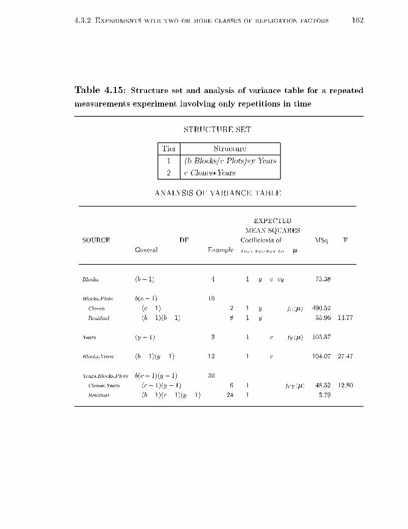
4.3.2 Experiments with two or more classes of replication factors 162
Table 4.15: Structure set and analysis of variance table for a repeated
measurements experiment involving only repetitions in time
STRUCTURE SET
Tier Structure
1 (b Blocks=c Plots)�y Years
2 c Clones�Years
ANALYSIS OF VARIANCE TABLE
EXPECTED
MEAN SQUARES
SOURCE DF CoeÆcients of MSq F
General Example �BPY �BP �BY �B �
Blocks (b� 1) 4 1 y c cy 75.38
Blocks.Plots b(c� 1) 10
Clones (c� 1) 2 1 y fC(�) 490.52
Residual (b� 1)(b� 1) 8 1 y 55.96 14.77
Years (y � 1) 3 1 c fY (�) 105.57
Blocks.Years (b� 1)(y � 1) 12 1 c 104.07 27.47
Years.Blocks.Plots b(c� 1)(y � 1) 30
Clones.Years (c� 1)(y � 1) 6 1 fCY (�) 48.52 12.80
Residual (b� 1)(c� 1)(y � 1) 24 1 3.79

4.3.2 Experiments with two or more classes of replication factors 163
derived according to the rules given in table 2.5, are as follows:
E[Y ] = Clones.Years
Var[Y ] = G + Blocks+ Blocks.Plots+ Blocks.Years + Blocks.Plots.Years
The analysis of variance table includes a source for Blocks.Years, about the inclusion
of which there has been some confusion in the literature. The usual justi�cation has
been that this interaction often occurs (see, for example, Anderson and Bancroft,
1952; Steel and Torrie, 1980). However, it is seen to be generally appropriate, in the
light of the structure set, to partition it out; to omit it, in any particular instance,
requires one to argue that it will not occur. Indeed, the analysis presented in table 4.15
reveals that for the generated data, Blocks.Years is a signi�cant source of variation.
As a result, the conclusions from the analysis given in table 4.15 di�er markedly from
those in table 4.14 in that a rather large interaction between Clones and Years has
been detected. This interaction was not detected in the split-plot analysis because
the Subplot Residual was in ated by the Blocks.Years component included in it.
Repetitions in time and space. Suppose that the experiment described in the
previous example was repeated at each of several sites. At �rst sight, one might be
tempted to think one had an experiment of the type described by Yates and Cochran
(see section 4.3.2.1) and, for an overall analysis of the data, to use that given in
table 4.13. However, the unrandomized factors in the experiment are Sites, Reps,
Plots and Years (that is, Years has not been randomized to Tracts of ground as in
the Yates-Cochran experiment). Clones is the only randomized factor. The structure
set for the experiment, a re ection of the experimental population and procedures,
and including a number of intertier interactions, is shown in table 4.16. Again, Sites
and Years are taken to be expectation factors as in the times-randomized-and-sites-
unrandomized experiment of section 4.3.2.1. The symbolic forms of the maximal
models for this experiment, derived according to the rules given in table 2.5, are as
follows:
E[Y ] = Clones.Sites.Years
Var[Y ] = G+ Sites.Blocks+ Sites.Blocks.Plots + Sites.Blocks.Years
+ Sites.Blocks.Plots.Years

4.3.2 Experiments with two or more classes of replication factors 164
Table 4.16: Structure set and analysis of variance table for an experiment
involving repetitions in time and space
STRUCTURE SET
Tier Structure
1 (s Sites=b Blocks=c Plots)�y Years
2 c Clones�Sites�Years
ANALYSIS OF VARIANCE TABLE
EXPECTED MEAN SQUARES
SOURCE DF CoeÆcients of
�SBPY �SBP �SBY �SB �CSY
Sites (s� 1) 1 y c cy fS(�CSY )
Sites.Blocks s(b� 1) 1 y c cy
Sites.Blocks.Plots sb(c� 1)Clones (c� 1) 1 y fC(�CSY )Clones.Sites (c� 1)(s� 1) 1 y fCS(�CSY )Residual s(b� 1)(c� 1) 1 y
Years (y � 1) 1 c fY (�CSY )
Sites.Years (s� 1)(y � 1) 1 c fSY (�CSY )
Sites.Blocks.Years (s� 1)(b� 1)(y � 1) 1 c
Sites.Blocks.Plots.Years sb(c� 1)(y � 1)Clones.Years (c� 1)(y � 1) 1 fCY (�CSY )Clones.Sites.Years (c� 1)(s� 1)(y � 1) 1 fCSY (�CSY )Residual s(b� 1)(c� 1)(y � 1) 1

4.3.2 Experiments with two or more classes of replication factors 165
The analysis of variance table for this experiment (also given in table 4.16) is
di�erent from the table given in table 4.13 in that the Residual of the latter has been
partitioned into two Residuals for the former. Thus the terms used for testing the
various hypotheses are di�erent for the two analyses.
Table 4.17: Experimental layout for a repeated measurements experi-
ment involving split plots and split blocks (Federer, 1975)y
Development StageBlock Herbicide
3 1 2I 7 6 3 5 2 1 4 1 4 6 2 7 3 5 5 6 3 1 7 2 4
A II 7 6 3 5 2 1 4 1 4 6 2 7 3 5 5 6 3 1 7 2 4
III 7 6 3 5 2 1 4 1 4 6 2 7 3 5 5 6 3 1 7 2 4
3 2 1III 3 2 1 6 4 5 7 5 4 2 3 7 6 1 6 2 4 3 7 5 1
B I 3 2 1 6 4 5 7 5 4 2 3 7 6 1 6 2 4 3 7 5 1
II 3 2 1 6 4 5 7 5 4 2 3 7 6 1 6 2 4 3 7 5 1
1 2 3III 3 6 2 5 1 4 7 6 3 7 5 4 2 1 1 2 6 4 7 3 5
C II 3 6 2 5 1 4 7 6 3 7 5 4 2 1 1 2 6 4 7 3 5
I 3 6 2 5 1 4 7 6 3 7 5 4 2 1 1 2 6 4 7 3 5
1 3 2II 7 2 3 5 1 4 6 7 6 3 2 4 1 5 1 4 5 6 3 2 7
D III 7 2 3 5 1 4 6 7 6 3 2 4 1 5 1 4 5 6 3 2 7
I 7 2 3 5 1 4 6 7 6 3 2 4 1 5 1 4 5 6 3 2 7
yThe levels of T are given inside the boxes.
Measurement of the several parts of a pasture. Federer (1975, example 7.4)
discusses a repeated measurements experiment involving repetitions in time and space
and for which the basic design is obtained by combining split-block and split-plot

4.3.2 Experiments with two or more classes of replication factors 166
design principles. There are three whole plot herbicide preconditioning treatments
(H) arranged in a randomized complete block design of four blocks each with three
rows. The blocks are further subdivided into three columns and the three levels of
a development stage factor (D) randomized to the columns within a block. Each
column is subdivided into seven subplots and a third factor (T ) randomized to them.
The experimental layout is shown in table 4.17. The produce of each of the 63 plots in
the experiment is divided into three parts (grass, legumes and weeds) and the weight
of each part for each plot recorded, giving 189 measurements.
The structure set for this experiment is as follows:
Tier Structure
1 (4 Blocks=(3 Rows�(3 Cols=7 Subplots)))�3 Parts
2 3 H�3 D�7 T�Parts

4.3.2 Experiments with two or more classes of replication factors 167
Table 4.18: Analysis of variance table for a repeated measurements ex-
periment involving split plots and split blocks
EXPECTED MEAN SQUARESSOURCE DF CoeÆcients of
�BRCSP �BCSP �BRP �BRCS �BCS �BR
�BRCP �BCP �BP �BRC �BC �B
Blocks 3 1 7 3 21 21 63 3 21 9 63 63 108
Blocks.Rows 8
H 2 1 7 21 3 21 63
Residual 6 1 7 21 3 21 63
Blocks.Cols 8
D 2 1 7 3 21 3 21 9 63
Residual 6 1 7 3 21 3 21 9 63
Blocks.Cols.Subplots 72
T 6 1 3 3 9
D.T 12 1 3 3 9
Residual 54 1 3 3 9
Blocks.Rows.Cols 16
H.D 4 1 7 3 21
Residual 12 1 7 3 21
Blocks.Rows.Cols.Subplots 144
H.T 12 1 3
H.D.T 24 1 3
Residual 108 1 3
Parts 2 1 7 3 21 21 63
Parts.Blocks 6 1 7 3 21 21 63
Parts.Blocks.Rows 16
Parts.H 4 1 7 21
Residual 12 1 7 21
Parts.Blocks.Cols 16
Parts.D 4 1 7 3 21
Residual 12 1 7 3 21
Parts.Blocks.Cols.Subplots 144
Parts.T 12 1 3
Parts.D.T 24 1 3
Residual 108 1 3
Parts.Blocks.Rows.Cols 32
Parts.H.D 8 1 7
Residual 24 1 7
Parts.Blocks.Rows.Cols.Subplots 288
Parts.H.T 24 1
Parts.H.D.T 48 1
Residual 216 1
yVariation contribution only to expected mean squares.

4.3.2 Experiments with two or more classes of replication factors 168
The analysis of variance is given in table 4.18.
In this experiment the unrandomized factor Parts is clearly an expectation factor.
The symbolic forms of the maximal models for this experiment, derived according to
the rules given in table 2.5, are as follows:
E[Y ] = Parts.H.D.T
Var[Y ] = G + Blocks+ Blocks.Rows + Blocks.Columns
+ Blocks.Columns.Subplots+ Blocks.Rows.Columns
+ Blocks.Rows.Columns.Subplots
+ Blocks.Parts + Blocks.Rows.Parts + Blocks.Columns.Parts
+ Blocks.Columns.Subplots.Parts + Blocks.Rows.Columns.Parts
+ Blocks.Rows.Columns.Subplots.Parts
The analysis given by Federer (1975) is given in table 4.19.
There are two major di�erences between the two analyses. First, the sources des-
ignated `error (HT)' and `error (HDT)' by Federer are not separated in the analysis
given in table 4.18; they are combined in the Residual source for Blocks.Rows.Cols.-
Subplots. Because of the sampling employed, their separation is not justi�ed. Second,
the source `error (Parts)' of Federer (1975, section 7.4), has been partitioned into the
Residual sources for the interactions involving Parts.Blocks in table 4.18. The analy-
sis presented in table 4.18 is quite di�erent from that obtained within the conventional
split-plot framework by Federer.

4.3.2 Experiments with two or more classes of replication factors 169
Table 4.19: Federer (1975) Analysis of variance table for a repeated
measurements experiment involving split plots and split blocks
SOURCE DF
Blocks 3H 2Blocks.H = error (H) 6D 2Blocks.D = error(D) 6T 6D.T 12Blocks.T.S = error(T) 54H.D 4Blocks.H.D = error(HD) 12H.T 12Blocks.H.T = error(HT) 36H.D.T 24Blocks.H.D.T = error(HDT) 72Parts 2Parts.H 4Parts.D 4Parts.T 12Parts.D.T 24Parts.H.D 8Parts.H.T 24Parts.H.D.T 48Blocks.Parts.H.D.T = error (Parts) 378

4.3.2 Experiments with two or more classes of replication factors 170
4.3.2.3 Factors randomized to two or more classes in bottom tier, no
carry-over
Subjects with repetitions in time. In a psychological experiment four subjects
of each sex participated in three blocks of four trials. In each block the subjects
were given two pairs of synonyms and two pairs of words unrelated in meaning. One
word of the pair was played through a headphone to the left ear and the other to the
right ear. The experimenter used three di�erent interstimulus intervals; that is, three
di�erent times between when the �rst word was played to the left ear and when the
second word was played. These were randomly assigned to the blocks of trials for each
subject. The order of the four word pairs used in the experiment was randomized and
this order used for all the interstimulus intervals and subjects. The subjects were
asked to press one of two buttons if the two words were synonyms and the other
button if they were unrelated. Two subjects of each sex chosen at random were asked
to use their left hand and the others to use their right hand (all subjects were right-
handed). The time taken from when the second word was played to when the buzzer
was pressed (the reaction time) was measured.
The unrandomized factors in this experiment are Sex, Subjects, Blocks and Trials;
the randomized factors are Hand, ISI (interstimulus interval), Relation and Pairs.
The structure set for the experiment is as follows:
Tier Structure
1 (2 Sex=4 Subjects=3 Blocks)�4 Trials
2 2 Hand�3 ISI�(2 Relation=2 Pairs)�Sex
The resulting analysis table is given in table 4.20. The symbolic forms of the
maximal models for this experiment, derived according to the rules given in table 2.5,
are as follows:
E[Y ] = Relations.Pairs.Hand.ISI.Sex
Var[Y ] = G+ Sex.Subjects + Sex.Subjects.Blocks + Trials
+ Sex.Trials+ Sex.Subjects.Trials
+ Sex.Subjects.Blocks.Trials

4.3.2 Experiments with two or more classes of replication factors 171
Table 4.20: Analysis of variance table for a repeated measurements ex-
periment with factors randomized to two classes of replication factors, no
carry-over e�ects
EXPECTED MEAN SQUARESy
SOURCE DF CoeÆcients of�XSBT �XST �XT �T �XSB �XS
Sex 1 1 3 12 4 12Sex.Subjects 6Hand 1 1 3 4 12Hand.Sex 1 1 3 4 12Residual 4 1 3 4 12
Sex.Subjects.Blocks 16ISI 2 1 4ISI.Sex 2 1 4Hand.ISI 2 1 4Hand.ISI.Sex 2 1 4Residual 8 1 4
Trials 3Relation 1 1 3 12 24Relation.Pairs 2 1 3 12 24
Sex.Trials 3Relation.Sex 1 1 3 12Relation.Pairs.Sex 2 1 3 12
Sex.Subjects.Trials 18Relation.Hand 1 1 3Relation.Hand.Sex 2 1 3Relation.Pairs.Hand 1 1 3Relation.Pairs.Hand.Sex 2 1 3Residual 12 1 3
Sex.Subjects.Blocks.Trials 48Relation.ISI 2 1Relation.ISI.Sex 2 1Relation.Hand.ISI 2 1Relation.Hand.ISI.Sex 2 1Relation.Pairs.ISI 4 1Relation.Pairs.ISI.Sex 4 1Relation.Pairs.Hand.ISI 4 1Relation.Pairs.Hand.ISI.Sex 4 1Residual 24 1
yVariation contribution only to the expected mean squares.

4.3.2 Experiments with two or more classes of replication factors 172
In the analysis, the intertier interactions between Sex and the other randomized
factors are to be partitioned out. Also, the factor Blocks, which is intrinsically crossed
with the other factors in the bottom tier, is nested within Subjects and Sex because
the order in which the interstimulus intervals were used was randomized for each
subject. However, Trials remains crossed with the other factors because the order of
presentation of the four word pairs was the same for all blocks and subjects.
The analysis given in table 4.20 di�ers from what would be obtained by analogy with
those given by Winer (1971) in that i) the randomized and unrandomized factors (for
example, Sex and Hand respectively) are distinguished, ii) the structure in the time
factors (Blocks and Trials) is fully recognized and iii) intertier interactions between
Subjects and ISI , Relation and Pairs are not included. Clearly, the randomization
procedures are re ected in the confounding pattern evident in the analysis table in
table 4.20.
4.3.2.4 Factors randomized to two or more classes in bottom tier, carry-
over
The experiments in this category are based on the change-over design, which is
a design in which measurements on experimental units are repeated and the treat-
ments are changed between measurements in such a way that the carry-over e�ects
of treatments can be estimated (Cochran and Cox, 1957, section 4.6a; John and Que-
nouille, 1977, section 11.4). The analysis described in this section is based on joint
work with W.B. Hall; this involved discussions during which the analysis for experi-
ments without preperiod, such as the animals-with-repetitions-in-time experiment,
was formulated. It was available in a manuscript submitted for publication in 1979
but Payne and Dixon (1983) have since indicated how the analysis can be performed
with GENSTAT 4.
Animals with repetitions in time. Cochran and Cox (1957, sections 4.61a and
4.62a) analyse the results from part of an experiment on feeding dairy cows. They
analysed the milk yield from a 6-week period for six cows that were fed a di�erent
diet in each of three periods. The order of the diets for each cow was obtained by

4.3.2 Experiments with two or more classes of replication factors 173
using two 3� 3 Latin square designs. The original experiment involved 18 cows and
utilized 6 squares; the 18 cows were divided into 6 sets so that the 3 cows in each set
were as similar as possible in respect to milk yielding ability (Cochran, Autrey and
Cannon, 1941). The pair of Latin squares used in the part of the experiment analysed
allows one to estimate the carry-over (or residual e�ects) of treatments in the period
immediately after they are applied. However, because there is no preperiod, carry-over
e�ects are not estimated from the �rst period.
Cochran and Cox point out that, in change-over experiments based on sets of Latin
squares, treatments are to be randomized to letters and rows and columns of the
squares are randomized. The experimenter has to decide whether to remove period
e�ects separately in each square, as is best if period e�ects are likely to di�er from
square to square; on the other hand, the experimenter might elect to remove overall
period e�ects. In the former case the squares are kept separate and the rows and
columns randomized separately in each square; in the latter, all columns are random-
ized and the rows are randomized across squares.
However, randomization of the rows of a single square can only be used when the
residual e�ects are balanced across a single square, as may be the case for an even
number of treatments. In the example from Cochran and Cox, a pair of squares
is required to achieve balance so that rows must be randomized across this pair of
squares.
The unrandomized factors are Sets, Cows and Periods. The structure for the
randomized factors is complicated by the fact that carry-over e�ects cannot occur
in measurements taken in the �rst period. This is overcome by introducing a factor
for no carry-over e�ect versus carry-over e�ect. That is, a factor (First) which is 1 for
the �rst period and 2 for other periods. The factor for carry-over e�ects (Carry) then
has four levels: 1 for no carry-over and 2, 3 and 4 for carry-over of the �rst, second
and third diets, respectively; however, the order of this factor is 3. The structure set
for the experiment is as follows:
Tier Structure
1 (2 Sets=3 Cows)�3 Periods
2 2 First=3 Carry+3 Direct

4.3.2 Experiments with two or more classes of replication factors 174
Table 4.21: Analysis of variance table for the change-over experiment
from Cochran and Cox (1957, section 4.62a)
EXPECTEDMEAN SQUARESy
SOURCE DF CoeÆcients of MSq F�SCP �SP �P �SC �S
Sets 1 1 3 3 9 18.00
Sets.Cows 4First.Carryz 2 1 3 2112.06 2.74Residual 2 1 3 769.50
Periods 2First 1 1 3 6 8311.36 2.62Residual 1 1 3 6 3168.75
Sets.Periods 2 1 3 4.50
Sets.Cows.Periods 8First.Carryx 2 1 19.21 0.39Direct{ 2 1 1427.28 28.65Residual 4 1 49.81
yVariation contribution only to the expected mean squares.zFirst.Carry is partially confounded with the Sets.Cows with eÆciency 0.167.xFirst.Carry is partially confounded with Sets.Cows.Periods with eÆciency 0.833.{Direct is partially aliased with First.Carry with eÆciency 0.800.
The relationship between First and Carry must be nested as it is impossible to have
no carry-over (level 1 of First) with carry-over from a dietary treatment (levels 2, 3
and 4 of Carry). The relationship between the carry-over factors and Direct (dietary
e�ect) must be independent because of the combinations of one diet following another.
This example does not ful�l the conditions given in section 2.2.5; there is no term

4.3.2 Experiments with two or more classes of replication factors 175
derived from the structure from the second tier to which all other terms from that
tier are marginal and, as Direct is not orthogonal to First.Carry , the experiment
is not structure balanced. However, with randomized factors being designated as
expectation factors, it is possible to use the approach to formulate an analysis, albeit
not a unique analysis. The symbolic forms of the maximal models for this experiment,
derived according to the rules given in table 2.5, are as follows:
E[Y ] = First.Carry + Direct
Var[Y ] = G + Sets + Sets.Cows + Periods + Sets.Periods
+ Sets.Cows.Periods
The analysis of variance table is given in table 4.21; it di�ers from that speci�ed
by Payne and Dixon (1983), and from that given by Cochran and Cox (1957), in
that here Periods is crossed with all �rst tier factors.. The First.Carry source in the
analysis table gives the di�erences between carry-over e�ects as it is orthogonal to
First. The analysis of variance was performed in GENSTAT 4 (Alvey et al., 1977).
Because the algorithm used to perform the analysis in GENSTAT 4 is sequential in
nature, the e�ect of having First and Carry before Direct in the structure is that
Direct is adjusted for First.Carry but not vice versa. By repeating the analysis with
Direct �rst in the formula, the analysis in which First.Carry is adjusted for Direct
will be obtained.
Experiment with preperiod. Kunert (1983) gives examples of change-over ex-
periments in which there is a preperiod so that residual e�ects are estimated from all
periods of the experiment. Such experiments have a somewhat simpler analysis than
those without preperiod, such as the animals-with-repetitions-in-time experiment just
discussed. For example, consider Kunert's (1983) example 4.7. The layout for this
experiment is given in table 4.22.
The unrandomized factors for this experiment are Units and Periods and the ran-
domized factors are Direct and Carry . The structure set is as follows:
Tier Structure
1 4 Units�12 Periods
2 3 Carry+3 Direct

4.3.2 Experiments with two or more classes of replication factors 176
Table 4.22: Experimental layout for a change-over experiment with pre-
period(Kunert, 1983)
PeriodsPreperiod 1 2 3 4 5 6 7 8 9 10 11 12
1 3 1 2 3 1 2 3 1 2 3 1 2 32 2 1 2 3 3 2 1 1 1 3 3 2 2
Units 3 3 2 3 1 1 3 2 2 2 1 1 3 34 1 3 1 2 2 1 3 3 3 2 2 1 1
The analysis of variance table is given in table 4.23. Again, this example does not
ful�l the conditions given in section 2.2.5; as for the previous example, there is no
term derived from the structure for the second tier to which all other terms derived
from that tier are marginal and, as Direct is not orthogonal to Carry , the experiment
is not structure balanced. But, with randomized factors again being designated as
expectation factors, it has been possible to use the approach to formulate a nonunique
analysis. The symbolic forms of the maximal models for this experiment, derived
according to the rules given in table 2.5, are as follows:
E[Y ] = Carry + Direct
Var[Y ] = G+ Units+ Periods+ Units.Periods

4.3.2 Experiments with two or more classes of replication factors 177
Table 4.23: Analysis of variance table for the change-over experiment
with preperiod from Kunert (1983)
EXPECTEDMEAN SQUARESy
SOURCE DF CoeÆcients of�UP �P �U
Units 3 1 12
Periods 11Carryz 2 1 4Residual 9 1 4
Units.Periods 33Carryx 2 1Direct{ 2 1Residual 29 1
yVariation contribution only to the expected mean squares.zCarry is partially confounded with the Periods with eÆciency 0.062.xCarry is partially confounded with Units.Periods with eÆciency 0.938.{Direct is partially aliased with Carry with eÆciency 0.938.

178
Chapter 5
Analysis of three-tiered
experiments
5.1 Introduction
In this chapter the analysis of three-tiered experiments is examined to illustrate how
the method described in chapter 2 facilitates their analysis. As is candidly acknowl-
edged in section 2.1, a satisfactory analysis for many studies can be formulated without
utilizing the proposed paradigm. However, it was suggested that the analysis of com-
plex experiments would be assisted if the approach is employed. This is particularly
the case for multitiered experiments; indeed, the full analysis of the experiment pre-
sented in section 5.2.4 can only be achieved with it. The analyses presented herein
di�er from those produced by other published methods so that, in some cases, I put
forward analyses that more closely follow generally accepted principles for the analysis
of designed experiments. Again, it will be assumed that the analyses discussed will
only be applied to data that conform to the assumptions necessary for them to be
valid.

5.2 Two-phase experiments 179
5.2 Two-phase experiments
Two-phase experiments were introduced by McIntyre (1955). They are commonly
used in the evaluation of wine (Ewart, Brien, Soderlund and Smart, 1985; Brien, May
and Mayo, 1987).
5.2.1 A sensory experiment
To introduce the analysis of two-phase experiments using the method presented herein,
the analysis of an orthogonal two-phase experiment is given in this section; the analysis
has been previously discussed by Brien (1983).
Consider an experiment to evaluate a set of wines made from the produce of a �eld
trial in order to test the e�ects of several viticultural treatments. Suppose that, in the
�eld trial, the treatments are assigned to plots according to a randomized complete
block design. The produce from each plot was separately made into wine which was
evaluated at a tasting in which several judges are given the wines over a number of
sittings. One wine is presented for scoring to each judge at a sitting and each wine is
presented only once to a judge. The order of presentation of the wines is randomized
for each judge. This experiment is then a two-phase experiment. In the �rst phase
the �eld trial is conducted, and in the second phase the wine made from the produce
of each plot in the �eld trial is evaluated by several judges.
The factors in the experiment are Blocks, Plots and Treatments from the �eld phase
of the experiment, and Judges and Sittings from the tasting phase. An observational
unit (of which there are jbt) is the wine given to a judge at a particular sitting.
The structure set is derived as described in section 2.2.4. Judges and Sittings are
the factors that would index the observational unit if no randomization had occurred,
and so these form the bottom tier of unrandomized factors. The �eld units, and
hence the wines, are uniquely identi�ed by the factors Blocks and Plots and they
would do so even if no randomization had been carried out in the �eld phase. As
the combinations of these factors were randomized to the sittings for each judge, they
form the second tier. The levels of Treatments were randomized to the plots within

5.2.1 A sensory experiment 180
each block and so Treatments forms the third or top tier. The structure set, assuming
no intertier interaction, is as follows:
Tier Structure
1 j Judges=bt Sittings
2 b Blocks=t Plots
3 t Treatments
The degrees of freedom of terms derived from the structure for a tier are computed,
as outlined in table 2.2, using the Hasse diagrams of term marginalities; the diagrams
for this example are given in �gure 5.1
Figure 5.1: Hasse diagram of term marginalities for a sensory experiment
��
��
��
��
��
��
6
6
�1 1
Judgesj j�1
Judges.Sittingsjbt j(bt�1)
��
��
��
��
��
��
6
6
�1 1
Blocksb b�1
Blocks.Plotsbt b(t�1)
��
��
��
��
6
�1 1
Treatmentst t�1
Tier 1 Tier 2 Tier 3
The analysis of variance table for this example, derived according to the rules given
in table 2.1, is given in table 5.1. The indentation of the Treatments source indicates

5.2.1 A sensory experiment 181
that Treatments is confounded with Blocks.Plots. The Residual source immediately
below the Treatments source corresponds to the unconfounded Blocks.Plots subspace,
that is, the unconfounded di�erences between plots within a block. Similarly, the
Blocks and Blocks.Plots sources are confounded with the Judges.Sittings source and
the second Residual source provides the unconfounded Judges.Sittings subspace.
Table 5.1: Analysis of variance table for a two-phase wine-evaluation
experiment
EXPECTED MEAN SQUARES
SOURCE DF CoeÆcients of�JS �J �BP �B �T
Judges j � 1 1 bt
Judges.Sittings j(bt� 1)Blocks (b� 1) 1 j jtBlocks.Plots b(t� 1)Treatments (t� 1) 1 j f(�T )Residual (b� 1)(t� 1) 1 j
Residual (j � 1)(bt� 1) 1
Total jbt� 1
For the purpose of determining the maximal expectation and variation models, all
factors, except for Treatments, are assumed to contribute to variation. The maximal
models for this experiment are derived as described in table 2.5 and, assuming the
data are lexicographically ordered on Judges and Sittings, are as follows:
E[y ] = �T
Var[y ] = V1 +V2
where

5.2.1 A sensory experiment 182
V1 = �GJ J+ �JI J + �JS I I,
V2 = U2(�BI J J+ �BP I I J)U02, and
U2 is the permutation matrix of order jbt re ecting the assigning of levels
combinations of Blocks and Plots to the sittings in which they were
presented to each judge.
The expected mean squares under this model, derived as described in table 2.8, are
also as given in table 5.1.
Figure 5.2: Minimal sweep sequence for a two-phase sensory experimenty
Residualz
Judges.Sittings
Judges
Blocks.Plots
Blocks
Residualz
Treatments
�� ��
�� ��
�� ��
�� ��
�� ��
�� ��
�� ��
?
?-
?-
?
yLines originating below a term signify a residual sweep and lines originating alongside a term signifya pivotal sweep (section 3.3.1.1).zResidual does not involve a sweep but merely serves to indicate the origin of the residuals for aresidual source.
The minimal sweep sequence for performing the analysis as prescribed in sec-
tion 3.3.1.1 is given in �gure 5.2.

5.2.1 A sensory experiment 183
Table 5.2: Analysis of variance table, including intertier interactions, for
a two-phase wine-evaluation experiment
EXPECTED MEAN SQUARESSOURCE DF CoeÆcients of
�JS �J �BPJ �BJ �BP �B �TJ �T
Judges j�1 1 bt 1 t b
Judges:Sittings j(bt�1)
Blocks (b�1) 1 1 t j jt
Blocks:P lots b(t�1)
Treatments (t�1) 1 1 j b f(�T )
Residual (b�1)(t�1) 1 1 j
Blocks:Judges (b�1)(j�1) 1 1 t
Blocks:P lots:Judges b(t�1)(j�1)
Treatments:Judges (t�1)(j�1) 1 1 b
Residual (b�1)(t�1)(j�1) 1 1
Total jbt� 1
It might be considered desirable to modify the structure set for the example to
include intertier interactions likely to arise. For this purpose, factors from lower tiers
have to be included in the structures for some higher tiers. An alternative structure
set for the example, involving such intertier interaction, is as follows:
Tier Structure
1 j Judges=bt Sittings
2 (b Blocks=t Plots)�Judges
3 t Treatments�Judges
The analysis derived from this structure set is given in table 5.2. This analysis is
quite di�erent from that presented in table 5.1; in particular, the test for Treatments
now involves a ratio of linear combinations of mean squares, whereas only a ratio

5.2.2 McIntyre's experiment 184
of mean squares is involved in table 5.1. Thus, it is possible that quite di�erent
conclusions will be reached depending on which analysis is performed.
5.2.2 McIntyre's experiment
In this section the method presented herein is applied to the nonorthogonal, but
structure-balanced, three-tiered experiment presented by McIntyre (1955). This illus-
trates the application to a more complicated experiment which results in an analysis
of variance table that is more informative than previously presented analysis tables
in that it re ects the randomization employed in the experiment. Further, there is
some clari�cation of which terms should be included in the analysis.
The object of the experiment was to investigate the e�ects of four light intensity
treatments on the synthesis of tobacco mosaic virus in the leaves of Nicotiana tabacum.
In the �rst phase of the experiment, Nicotiana leaves, inoculated with virus, were
subjected to the four di�erent light intensities. The experimental arrangement for
the �rst phase was obtained using two 4 � 4 Latin square designs, the rows and
columns of these squares corresponding to Nicotiana plants and position of the leaves
on these plants; the two Latin squares corresponded to di�erent sets of Nicotiana
plants. The layout is illustrated in �gure 5.3.
In the second phase sap from each of the leaves of the �rst phase was injected
into a half-leaf of the assay plant, Datura stramonium. The assignment of �rst-phase
leaves to the half-leaves of the assay plants was accomplished using four Graeco-Latin
squares; the rows and columns of the squares corresponded to Datura plants and
position of the leaf on the assay plants, respectively. Within a Graeco-Latin square,
the four leaves from one Nicotiana plant from each set were assigned to the half-leaves
of the assay plant using the one alphabet for each plant. The layout is illustrated in
�gure 5.4.

5.2.2 McIntyre's experiment 185
Figure 5.3: Layout for the �rst phase of McIntyre's (1955) experimenty
Nicotiana Plants1 2 3 4 1 2 3 4
Leaf LeafPosition Position
a b c d a b c d1 1
1 5 9 13 17 21 25 29b a d c c d a b
2 22 6 10 14 18 22 26 30c d a b d c b a
3 33 7 11 15 19 23 27 31d c b a b a d c
4 44 8 12 16 20 24 28 32
yThe letter in each cell refers to the light intensity to be applied to the unit and the number to theunit.

5.2.2 McIntyre's experiment 186
Figure 5.4: Layout for the second phase of McIntyre's (1955) experimenty
Datura Plants1 2 3 4 5 6 7 8
Assay Leaf Assay LeafPosition Position
1 2 3 4 5 6 7 81 1
17 20 18 19 23 22 24 212 1 4 3 8 7 6 5
2 218 19 17 20 22 23 21 243 4 1 2 7 8 5 6
3 319 18 20 17 21 24 22 234 3 2 1 6 5 8 7
4 420 17 19 18 24 21 23 22
Datura Plants9 10 11 12 13 14 15 16
Assay Leaf Assay LeafPosition Position
9 10 11 12 13 14 15 161 1
28 25 27 26 30 31 29 3210 9 12 11 16 15 14 13
2 227 26 28 25 31 30 32 2911 12 9 10 15 16 13 14
3 326 27 25 28 32 29 31 3012 11 10 9 14 13 16 15
4 425 28 26 27 29 32 30 31
yThe numbers in the cell refer to the units from the �rst phase to be assigned to the two half-leavesof the assay plant.

5.2.2 McIntyre's experiment 187
The observational unit is a half leaf of an assay plant and the factors in the experi-
ment are Reps, Datura, APosition, Halves, Sets, Nicotiana, Position and Treatments.
The structure set for this experiment, derived using the steps given in section 2.2.4,
is as follows:
Tier Structure
1 ((4 Reps=4 Datura)�4 APosition)=2 Halves
2 (2 Sets=4 Nicotiana)==Nicotiana
+(Sets/Nicotiana)�4 Position
3 4 Treatments
The structures derived from the factors in tiers two and three correspond to the
structure set for the �rst phase of the experiment, while the structure derived from
bottom tier factors corresponds to the structure of the units from the second phase.
Note that Nicotiana has to be included as a pseudoterm to Sets.Nicotiana for the
correct degrees of freedom to be obtained using the method described in table 2.2.
The pseudofactor indexes which Nicotiana plants from the �rst phase were assigned
to the same Datura plant in the second phase.
The analysis of variance for the experiment, obtained using the rules given in ta-
ble 2.1, is given in table 5.3. The Hasse diagrams of term marginalities, used in
obtaining the degrees of freedom of the terms in the analysis table as prescribed in
table 2.2, are presented in �gure 5.5.
For the purpose of deriving the maximal expectation and variation models for the
experiment, it is likely that all factors in the experiment, other than Treatments, will
be classi�ed as variation factors. Thus, the application of the steps given in table 2.5
yields the following models for the experiment, assuming the data are lexicographically
ordered on Reps, Datura, APosition, and Halves:
E[y ] = �T
Var[y ] = V1 +V2
where

5.2.2 McIntyre's experiment 188
Figure 5.5: Hasse diagram of term marginalities for McIntyre's experi-
ment
��
��
��
��
��
����
��
��
����
��
����
6
@@
@I
����
HHHH
HHY6 6
@@
@I
����
�1 1
APo4 3
Rep4 3
Rep.APo16 9
Rep.Dat16 12
Rep.Dat.APo64 36
Rep.Dat.APo.Half128 64
��
��
����
6
�1 1
Treatments4 3
��
��
��
����
��
��
����
����
��
����
@@
@I
����
PPPP
PPPP
Pi
HHHH
HHY6 6
����
����
�16
PPPP
PPPP
Pi
�1 1
Pos4 3
Set2 1
Nic4 3
Set.Pos8 3
Set.Nic8 3
Set.Nic.Pos32 18
Tier 1
Tier 3
Tier 2

5.2.2 McIntyre's experiment 189
Table 5.3: Analysis of variance table for McIntyre's two-phase experi-
ment
EXPECTED MEAN SQUARESSOURCE DF CoeÆcients of MSq F
�RADH �RDA �RA �A �RD �R �SNP �SN �SP �S �P �T
Reps 3
Sets.Nicotiana 3 1 2 8 8 32 4 16 182.58
Reps.Datura 12 1 2 8 75.12 6.37
APosition 3 1 2 8 32 119.07 14.87
Reps.APosition 9 1 2 8 8.01 0.68
Reps.Datura.APosition 36
Positiony 3 1 2 2 8 16 36.95 0.91
Sets.Positiony 3 1 2 2 8 40.47 1.30
Sets.Nicotiana.Positiony 18
Treatmentsy 3 1 2 2 f(�T ) 74.12 2.38
Residual 15 1 2 2 31.14 2.64
Residual 12 1 2 11.80
Reps.Datura.APosition.Halves 64
Sets 1 1 4 16 16 64 41.40
Sets.Nicotianaz 3 1 4 16 10.30
Positiony 3 1 2 8 16 23.38 0.54
Sets.Positiony 3 1 2 8 43.31 4.31
Sets.Nicotiana.Positiony 18
Treatmentsy 3 1 2 f 0(�T ) 31.23 3.11
Residual 15 1 2 10.04
Residual 36 1 7.60
Total 127
yThese sources are partially confounded with eÆciency 0.50.zThe restrictions placed on randomization result in the subspace of Sets.Nicotiana confounded withReps being orthogonal to that confounded with Reps.Datura.APosition.Halves. Sets.Nicotiana isthus orthogonal to all �rst tier sources.

5.2.2 McIntyre's experiment 190
V1 = �GJ J J J+ �RI J J J+ �RDI I J J
+�AJ J I J+ �RAI J I J+ �RDAI I I J
+�RDAHI I I I,
V2 = U2(�PJ J I J + �SI J J J+ �SP I J I J
+�SNI I J J+ �SNP I I I J)U02, and
U2 is a permutation matrix of order 128 re ecting the assignment of the
levels combinations of Set, Nicotiana and Position to the halves.
Based on these models, the expected mean squares, which are also given in table 5.3,
are derived using the steps given in table 2.8.
The analysis di�ers from that given by Curnow (1959) only in its layout and in
that the Reps.APosition interaction has been isolated. The advantage of the lay-
out of the analysis table presented in table 5.3 is that the confounding between
sources in the table is obvious. For example, Treatments has been confounded with
Sets.Nicotiana.Position which, in turn, is confounded with both Reps.Datura.APosi-
tion and Reps.Datura.APosition.Halves. In respect, of the Reps.APosition interaction,
Curnow (1959) has combined this source with the Reps.Datura.APosition Residual
source in the `Residual (2)' of his Sums analysis. Also, the Reps.APosition interaction
is not `of the character of a treatment and block interaction' as suggested by Curnow,
but is a source contributing to variation that can be separated from the Residual.
The sums of squares were computed using the sweep sequence presented in �g-
ure 5.6. The directly nonorthogonal terms in the experiment are Positions, Sets.Po-
sitions and Sets.Nicotiana.Positions and these terms are structure balanced. In addi-
tion, the nonorthogonality of the last term induces nonorthogonality in the Treatments
term which must be taken into account in the analysis sequence. Since most terms
are orthogonal, most backsweeps are redundant and the sequence shown in �gure 5.6
is the minimal sequence.

5.2.2 McIntyre's experiment 191
Figure 5.6: Minimal sweep sequence for McIntyre's two-phase
experimenty
�� ���� ���� ���� ���� ��
?
?
?
?
Rep
Rep.Dat
APo
Rep.APo
Rep.Dat.APo
-�� ���� ��?
Set.Nic
Residualz
-�� ��Posx
? �� ��-Rep.Dat.APo
Set.Posx
? �� �� �� ��- - -Rep.Dat.APo
Set.Nic.Posx
Rep.Dat.APo
Treatx
? �� ��- - -Rep.Dat.APo
Set.Nic.Posx
Rep.Dat.APo
Residualz
? �� ��-Rep.Dat.APo
Residualz
?�� ��Rep.Dat.APo.Half
-�� ���� ���� ���� ���� ���� ��
?
?
?
?
?
?
?
?
Set
Set.Nic
Posx
Rep.Dat.APo
Set.Posx
Rep.Dat.APo
Set.Nic.Posx
Rep.Dat.APo
Residualz
-
�� ���� ��
?
?
?
Rep.Dat.APo
Treatx
Rep.Dat.APo
Set.Nic.Posx
-
�� ��?
Rep.Dat.APo
Residualz
yLines originating below a term signify a residual sweep and lines originating alongside a term signify a pivotal sweep (section 3.3.1.1).Terms placed in dashed boxes signify a backsweep (section 3.3.1.1).zResidual does not involve a sweep but merely serves to indicate the origin of the residuals for a residual source.xFor these sources e�ective means are calculated by dividing computed means by an eÆciency factor of 0.5.

5.2.3 Taste-testing experiment from Wood, Williams and Speed (1988) 192
5.2.3 Taste-testing experiment from Wood, Williams and
Speed (1988)
Wood, Williams and Speed (1988) in their discussion of two-phase experiments claim
that they provide an analysis of variance table which is very similar to that put
forward by Brien (1983). In this section, I illustrate how the analysis of variance
table produced using the method outlined herein di�ers from that presented by Wood
et al. (1988). As a result, it will become clear that their partition of the Total sum
of squares may not be correct and that a more informative analysis of variance table
can be produced. Also, from the discussion of this example, it will be evident how
di�erences in the layout of an experiment might a�ect the analysis and, hence, be
re ected in the analysis of variance table. The analyses presented in this section are
all structure balanced.
The Wood et al. (1988) experiment with which we are concerned is their second
example, a taste-testing experiment the purpose of which was to investigate the e�ects
of six storage treatments on milk drinks. The experiment was a two-phase experiment;
in the �rst or storage phase, the milk drinks were subjected to the storage treatments,
whilst in the second or tasting phase, tasters scored the produce from the storage
phase. The storage treatments were the six combinations of two types of container
(plastic, glass) and three temperatures (-20ÆC, 1ÆC, 30ÆC).
A problem encountered at the outset in deriving the analysis for this semiconstruct-
ed example, is that, as I shall elaborate later in this section, the design used in the
�rst phase could not have been as described by Wood et al. (1988). However, the fol-
lowing scenario does �t with the Wood et al. (1988) description in that a randomized
complete block design is utilized in the assignment of treatment combinations in the
�rst phase.
Suppose that the �rst phase of the experiment involved treating milk rather than
storing it. In each of two periods six runs were performed; at each run the milk was
treated at one of the three temperatures mentioned above while contained in either
the plastic or glass container. After processing, six samples, corresponding to the six
type-temperature combinations, were randomly presented to 8 judges in each of two

5.2.3 Taste-testing experiment from Wood, Williams and Speed (1988) 193
sessions. This experiment will be referred to as the Wood, Williams and Speed (1988)
processing experiment. The data from the experiment are presented in table 5.4.
Table 5.4: Scores from the Wood, Williams and Speed (1988) processing
experimenty
Session 1 2Type Plastic Glass Plastic GlassTemperature -20 1 30 -20 1 30 -20 1 30 -20 1 30
Judge
1 4 5 5 6 3 5 5 6 7 7 4 72 6 6 7 5 6 7 4 7 6 5 6 63 4 7 8 8 2 8 2 8 3 8 7 74 6 6 7 5 3 4 2 5 1 6 2 35 7 7 7 7 7 7 7 7 8 7 8 86 7 8 8 6 5 7 8 6 7 7 8 87 7 7 7 6 6 6 6 6 6 8 8 68 7 7 7 6 6 6 6 6 6 8 8 6
yThe bolded scores are from the second period
The observational unit for this experiment is a unit scored by a judge in a session.
The factors are Judge, Session, Unit, Period, Run, Type and Temperature. The
factors that would index the observational unit if no randomization had occurred are
Judge, Session and Unit so these form the bottom or unrandomized tier. The factors
Period and Run index uniquely the �rst-phase units and would index the �rst-phase
units if no randomization had occurred in that phase. Hence, these factors form
the second tier of factors. The third tier is comprised of Type and Temperature as
these were assigned randomly to runs within each period. The structure set derived
from these tiers is as follows, it being necessary to include pseudofactors to obtain a
structure-balanced set of terms:

5.2.3 Taste-testing experiment from Wood, Williams and Speed (1988) 194
Tier Structure
1 (8 Judge�2 Session)=6 Unit
2 (2 Period=6 Run)==(2 Pseudo*Temperature)
3 2 Type�3 Temperature
The pseudofactor Pseudo is a factor of two levels. Observations that take level
1 of Pseudo are those with the levels combinations 1,1 and 2,2 of Period and Type,
otherwise an observation takes level 2 of Pseudo. The pseudoterms identify the various
subspaces of Period.Run that have the same eÆciency factors relative to the tier 1
structure (see table 5.5).
The degrees of freedom of terms derived from the structure for a tier are computed,
as outlined in table 2.2, using the Hasse diagrams of term marginalities; the diagrams
for this example are given in �gure 5.7. The analysis of variance table for this example,
derived according to the rules given in table 2.1, is given in table 5.5.
Assume all factors in the experiment, except Type and Temperature, are to be
designated as variation factors. The symbolic form of the maximal models for this
experiment, derived according to the rules given in table 2.5, is as follows:
E[Y ] = Type.Temperature
Var[Y ] = G+ Judge + Session+ Judge.Session + Judge.Session.Unit
+ Period+ Period.Run
Note that it may not be appropriate to designate Judge as a variation factor. This
is because judges evaluate in an individualistic manner and it will be important to
compare one judge's evaluation with another's; this is certainly the case with wine
evaluation (Brien, May and Mayo, 1987). However, in order to conform with Wood
et al. (1988), Judge will remain a variation factor.
The expected mean squares based on the above model are also given in table 5.5.
In computing these, one had �rst to derive the expectation for each of the mean
squares that would have been obtained if terms arising from pseudoterms had not
been combined. The expectation of a combined mean square was then obtained
as the weighted average of the expectation of the mean squares comprising it, the
weights being the degrees of freedom of the mean squares. Thus, the expectation of

5.2.3 Taste-testing experiment from Wood, Williams and Speed (1988) 195
Figure 5.7: Hasse diagram of term marginalities for the Wood, Williams
and Speed (1988) processing experiment
��
��
��
��
��
����
��
��
��
6
@@
@I
����
@@
@I
����
�1 1
Judge8 7
Session2 1
Judge.Session16 7
Judge.Session.Unit96 80
��
��
��
����
��
��
��
@@
@I
����
@@
@I
����
�1 1
Temp3 2
Type2 1
Type.Temp6 2
��
��
��
��
��
����
����
��
��
��
ZZ
ZZ
ZZ
ZZ
ZZ
ZZ}
����
��*
����
��*
HHHH
HHY
����
����
�16
PPPP
PPPP
Pi
�1 1
Period2 1
Pseudo2 1
Temp3 2
Pseudo.Temp6 2
Period.Run12 5
Tier 1
Tier 2
Tier 3

5.2.3 Taste-testing experiment from Wood, Williams and Speed (1988) 196
Table 5.5: Analysis of variance table for Wood, Williams and Speed
(1988) processing experiment
ANALYSIS OF VARIANCE TABLE
EXPECTED MEAN SQUARES
SOURCE DF CoeÆcients of MSq�JSU �JS �S �J �PR �P
Judge 7 1 6 12 12.213
Session 1 1 6 48 0.010
Judge.Session 7Period.Run 3 1 6 8
33.066
Residual 4 1 6 2.719
Judge.Session.Unit 80Period 1 1 8 48 1.260Period.Run 10Type 1 1 8 0.094Temperature 2 1 8 0.667Type.Temperature 2 1 8 8.000Residual 5 1 32
50.909
Residual 69 1 1.735
Total 95
INFORMATION SUMMARY
Model term EÆciency
Judge.SessionPseudo 1
3
Pseudo.Temp 13
Judge.Session.UnitPseudo 2
3
Pseudo.Temp 23

5.2.3 Taste-testing experiment from Wood, Williams and Speed (1988) 197
Figure 5.8: Minimal sweep sequence for Wood, Williams and Speed
(1988) processing experimenty
�� ���� ���� ��?
?
Judge
Session
Judge.Session
�� ��?Judge.Session.Unit
-�� ���� ��?
Pseudox
Judge.Session -�� ���� ��?
Pseudo.Tempx
Judge.Session -�� ��Residualz
-�� ���� ���� ���� ���� ��
?
?
?
?
?
?
Period
Pseudox
Judge.Session
Temp
Pseudo.Tempx
Judge.Session
Period.Run
�� ��?
Residualz
- Judge.Session
?
-
?
Judge.Session
? -�� ���� ���� ���� ��
?
?
?
Type
Temp
Type.Temp
Residualz
yLines originating below a term signify a residual sweep and lines originating alongside a term signify a pivotal sweep(section 3.3.1.1). Where there are multiple inputs, the original e�ects are added together to form the input for thesweep to be performed at the destination. Terms placed in dashed boxes signify a backsweep (section 3.3.1.1).zResidual does not involve a sweep but merely serves to indicate the origin of the residuals for a residual source.xFor this source e�ective means are calculated by dividing computed means by an eÆciency factor which is given intable 5.5.

5.2.3 Taste-testing experiment from Wood, Williams and Speed (1988) 198
the Period.Run Residual mean square is
2(�JSU + 8�PR) + 3(�JSU + 163�PR)
2 + 3= �JSU +
32
5�PR
The sums of squares were computed using the sweep sequence presented in �g-
ure 5.8.
As I mentioned earlier in this section, the actual physical conduct of the experiment
will mean that it is unlikely that the assignment of treatment combinations in the
�rst phase could have been achieved using a randomized complete block design with
replicates corresponding to the blocks. This is because it was a storage experiment,
with the milk being stored in either plastic or glass containers; thus, there would
have to have been several containers of each type (3 if there were no replicates or 6
otherwise) and types could not have been randomly assigned to containers. On the
other hand, Temperatures would have been randomized to the di�erent containers
which may or may not have been blocked into two replicates. We will presume that
they were blocked and refer to this experiment as the Wood, Williams and Speed
(1988) storage experiment.
The factors are Judge, Session, Unit, Rep, Type, Container and Temperature.
The factors that would index the observational unit if no randomization had been
performed are Judge, Session and Unit so these form the bottom or unrandomized
tier. The factors Rep, Type and Container index uniquely the �rst-phase units and
would index the �rst-phase units if no randomization had been performed in that
phase. Hence, these factors form the second tier of factors. The third tier is comprised
of Temperature as this was assigned randomly to containers within each rep-type
combination. The structure set derived from these tiers is as follows, it again being
necessary to include the pseudoterms to obtain a balanced analysis:
Tier Structure
1 (8 Judge�2 Session)=6 Unit
2 (2 Rep�2 Type)==2 Pseudo=6 Container)==(Pseudo*Temperature)
3 Type�3 Temperature

5.2.3 Taste-testing experiment from Wood, Williams and Speed (1988) 199
Table 5.6: Analysis of variance table for the Wood, Williams and Speed
(1988) storage experiment
ANALYSIS OF VARIANCE TABLE
EXPECTED MEAN SQUARESSOURCE DF CoeÆcients of MSq
�JSU �JS �S �J �RTC �RT �R
Judge 7 1 6 12 12.213
Session 1 1 6 48 0.010
Judge.Session 7Rep.Type 1 1 6 8
3243
6.420Rep.Type.Container 2 1 6 8
31.389
Residual 4 1 6 2.719
Judge.Session.Unit 80Rep 1 1 8 24 48 1.260Type 1 1 8 24 0.094Rep.Type 1 1 16
3483
2.778Rep.Type.Container 8Temperature 2 1 8 0.667Type.Temperature 2 1 8 8.000Residual 4 1 20
30.441
Residual 69 1 1.735
Total 95
INFORMATION SUMMARY
Model term EÆciency
Judge.SessionPseudo 1
3Pseudo.Temp 1
3
Judge.Session.UnitPseudo 2
3Pseudo.Temp 2
3

5.2.3 Taste-testing experiment from Wood, Williams and Speed (1988) 200
Figure 5.9: Minimal sweep sequence for the Wood, Williams and Speed
(1988) storage experimenty
�� ���� ���� ��?
?
Judge
Session
Judge.Session
�� ��?Judge.Session.Unit
-�� ���� ��?
Rep.Typex
Judge.Session -�� ���� ��?
Pseudo.Tempx
Judge.Session -�� ��Residualz
-�� ���� ���� ���� ���� ���� ��
?
?
?
?
?
?
?
Rep
Type
Rep.Typex
Judge.Session
Temp
Pseudo.Tempx
Judge.Session
Rep.Type.Contain
�� ��?
Residualz
?
-
?
Judge.Session
-�� ���� ���� ��
?
?
Temp
Type.Temp
Residualz
yLines originating below a term signify a residual sweep and lines originating alongside a term signify a pivotal sweep(section 3.3.1.1). Where there are multiple inputs, the original e�ects are added together to form the input for thesweep to be performed at the destination. Terms placed in dashed boxes signify a backsweep (section 3.3.1.1).zResidual does not involve a sweep but merely serves to indicate the origin of the residuals for a residual source.xFor this source e�ective means are calculated by dividing computed means by an eÆciency factor which is given intable 5.6.

5.2.3 Taste-testing experiment from Wood, Williams and Speed (1988) 201
The analysis of variance table for this example, derived according to the rules given
in table 2.1, is given in table 5.6.
Again, assume all factors in the experiment, except Type and Temperature, are to
be designated as variation factors. The symbolic form of the maximal models for the
storage experiment, derived according to the rules given in table 2.5, is as follows:
E[Y ] = Type.Temperature
Var[Y ] = G+ Judge + Session+ Judge.Session + Judge.Session.Unit
+ Rep + Rep.Type + Rep.Type.Container
The expected mean squares based on the above model are also given in table 5.6.
Again, the expectation of the Rep.Type.Container Residual mean square had to be
obtained as the weighted average of the expectations of the mean squares of which it
is comprised. It is calculated as follows:
2(�JSU + 8�RTC) + 2(�JSU + 163)
2 + 2= �JSU +
20
3�RTC
The sums of squares were computed using the sweep sequence presented in �g-
ure 5.9.
Comparison of the tables that I have produced (tables 5.5 and 5.6) with that pre-
sented by Wood et al. (1988) (see table 5.7) reveals a number of di�erences.
Firstly, their table gives no indication of the �rst phase units to which the types and
temperatures were randomized. Consequently, the term with which Type, Tempera-
ture and Type.Temperature is confounded has been omitted from each of the tables,
whereas in table 5.5 it is clear that these terms are confounded with Period.Run and,
in table 5.6, that the last two terms are confounded with Rep.Type.Container.
Secondly, there is no suggestion in the Wood et al. (1988) table of the Replicate
interactions with Type and Temperature being intertier interactions, which they are,
except for Rep.Type in the storage experiment. However, it is usual to assume there
are not such interactions and, if required to facilitate the analysis, they are only
included as pseudoterms or terms with no scienti�c interpretation. Further, as Brien
(1983) suggests the intertier interactions of Type and Temperature with Judge are
more likely to be important in taste-testing experiments. But, if it is thought that the

5.2.3 Taste-testing experiment from Wood, Williams and Speed (1988) 202
Table 5.7: Analysis of variance table after that presented by Wood,
Williams and Speed (1988) for a taste-testing experiment
ANALYSIS OF VARIANCE TABLE
EXPECTED MEAN SQUARESSTRATUM DF CoeÆcients of MSq
�JSU �JS �S �J �RTyTe �RTy �RTe �R
Judge 7 1 6 12 12.213
Session 1 1 6 48 0.010
Judge.Sessionreplicate.type 1 1 6 8
3243
6.420replicate.type.temperature 2 1 6 8
31.389
residual 4 1 6 2.719
Judge.Session.Unitreplicate 1 1 8 24 16 48 1.260type 1 1 8 24 0.094temperature 2 1 8 16 0.667type.temperature 2 1 8 8.000replicate.type 1 1 16
3483
2.778replicate.temperature 2 1 8 16 0.542replicate.type.temperature 2 1 16
30.340
residual 69 1 1.753
INFORMATION SUMMARY
Model term EÆciency factor
Judge.Session stratumreplicate.type 1
3replicate.type.temperature 1
3
Judge.Session.Unit stratumreplicate.type 2
3replicate.type.temperature 2
3

5.2.3 Taste-testing experiment from Wood, Williams and Speed (1988) 203
Replicate interactions might occur, one can include them, in addition to Period.Run
or Rep.Type.Container. Wood et al. (1988) provide no such rationale and it would
seem that they included them as full terms merely as a device to obtain a balanced
analysis. In these circumstances, they are more correctly designated as pseudoterms.
An important consequence of not including the Replicate interactions is that the
partition of the Total sum of squares di�ers so that divisors for F-test and estimates
of standard errors will di�er. In particular, the Period.Run Residual mean square
from the storage experiment can be obtained by pooling the replicate.type, repli-
cate.temperature and replicate.type.temperature mean squares from the Wood et al.
(1988). The Rep.Type.Container Residual mean square from the processing experi-
ment can be obtained by pooling the replicate.temperature and replicate.type.tem-
perature mean squares from the Wood et al. (1988) analysis.
Finally, Wood et al. (1988) assert that a problem in using the analysis-of-variance
method to obtain estimates of the canonical covariance components is that there are
usually more equations than parameters to estimate. This is not the case for this
example, nor for any of the other examples presented in the thesis.
In summary, of the analyses I have presented, the one most like that of Wood et al.
(1988) is surprisingly not that for the experiment employing the same design as theirs,
that is, the processing experiment based on a randomized complete block design in
the �rst phase. Rather, it is most like the storage experiment. Table 5.6 contains
almost the same set of mean squares as those in the Wood et al. (1988) table. The
di�erences are that the Rep.Type.Container Residual mean square consists of two
mean squares from the Wood et al. (1988) analysis and that the mean squares are
labelled di�erently to those in the Wood et al. (1988) table so that the types of
variability (section 6.6.2) contributing to the subspace are more accurately portrayed.
I believe this example demonstrates the advantage of employing the paradigm I have
proposed in the case of complex experiments. It provides a framework for deciding
which terms to include in the analysis that has to do with the behaviour expected
in the data rather than basing the decision on which terms are required to achieve a
balanced analysis.

5.2.4 Three structures required 204
5.2.4 Three structures required
In this section, a constructed structure-balanced example is presented, the experiment
being one that requires three structures for a complete analysis.
Consider a two-phase experiment (McIntyre, 1955) consisting of �eld and wine
evaluation phases. Suppose that the �eld phase involved a viticultural experiment to
investigate di�erences between four types of trellising and two methods of pruning.
The design consisted of two adjacent Youden squares of three rows and four columns,
the plots of which were each split into two subplots (or halfplots). Trellis was assigned
to main plots as shown in table 5.8 and methods of pruning were assigned at random
independently to the two halfplots within each main plot.
Table 5.8: Assignment of the trellis treatment to the main plots in the
�eld phase of the experiment.
Squares1 2
Columns 1 2 3 4 1 2 3 4
Rows1 4 1 2 3 2 1 4 32 1 2 3 4 3 2 1 43 2 3 4 1 4 3 2 1
For the evaluation phase, there were six judges all of whom took part in 24 sittings.
In the �rst 12 of these sittings the wines made from the halfplots of one square were
evaluated; the �nal 12 sittings were to evaluate the wines from the other square. At
each sitting, each judge assessed two glasses of wine from each of the two halfplots
of one of the main plots. The main plots allocated to the judges at each sitting
are shown in table 5.9, and were determined as follows. For the allocation of rows,
each occasion was subdivided into 3 intervals of 4 consecutive sittings. During each
interval, each judge examined plots from one particular row, these being determined

5.2.4 Three structures required 205
Table 5.9: Assignment of the main plots (Row and Column combinations)
from the �eld experiment to the judges at each sitting in the evaluation
phase.
Occasion 1Intervals 1 2 3Sittings 1 2 3 4 1 2 3 4 1 2 3 4
Judges1 13 12 11 14 31 34 32 33 22 23 24 212 23 22 21 24 11 14 12 13 32 33 34 313 33 32 31 34 21 24 22 23 12 13 14 114 31 34 33 32 22 23 21 24 13 12 11 145 11 14 13 12 32 33 31 34 23 22 21 246 21 24 23 22 12 13 11 14 33 32 31 34
Occasion 2Intervals 1 2 3Sittings 1 2 3 4 1 2 3 4 1 2 3 4
Judges1 24 21 22 23 31 33 32 34 11 13 12 142 14 11 12 13 21 23 22 24 31 33 32 343 34 31 32 33 11 13 12 14 21 23 22 244 33 32 31 34 13 11 14 12 24 22 23 215 23 22 21 24 33 31 34 32 14 12 13 116 13 12 11 14 23 21 24 22 34 32 33 31

5.2.4 Three structures required 206
using two 3 � 3 Latin square designs, one for judges 1{3 and the other for judges
4{6. Thus, for example, judge 1 examined plots from row 1 during interval 1 of the
�rst occasion, plots from row 3 during interval 2, and from row 2 during interval 3.
As a result, di�erences between judges and intervals could be eliminated from row
di�erences. At each sitting judges 1{3 examined wines from one particular column
and judges 4{6 examined wines from another column. Taking the 12 sittings from
each occasion, the ordered pairs of columns allocated to the two sets of judges were
chosen to ensure, �rstly, that each possible ordered combination of two out of four
columns occurred exactly once, and, secondly, that each judge examined a plot from
every column during each interval. Thus, judge di�erences could be eliminated from
column and row-column comparisons, and hence trellis di�erences; also, the amount
of information on row-column comparisons, and hence trellis di�erences, remaining
after sitting di�erences are eliminated is maximized. For clarity, table 5.9 shows the
plan in unrandomized order; in reality there would be a random permutation of the
numberings of the intervals within each occasion, the sittings within each interval,
and the judges on each occasion. Likewise, for each judge-sitting combination, the
positions (on the table) of the four glasses containing the two replicate wines from the
two halfplots were also randomized. Appendix A.4 contains such a randomized plan
together with a set of computer-generated scores. These scores are based on sum of a
set of e�ects, each of which is generated from a normal distribution; the sum was then
rounded to the nearest multiple of 0.5. This produces scores that take similar values
to those that would be obtained in practice. It is presumed that their distribution
is suÆciently close to being normal so that the analysis of variance is approximately
valid.
The observational unit for the experiment is a glass of wine in a position at a
sitting to be evaluated by an evaluator. The factors in the experiment are Occasions,
Intervals, Sittings, Judges, Positions, Rows, Squares, Columns, Halfplots, Trellis and
Method.
The structure set is derived as described in section 2.2.4. Three tiers are required
for this experiment and the structure set based on these is as follows:

5.2.4 Three structures required 207
Tier Structure
1 ((2 Occasions=3 Intervals=4 Sittings)�6 Judges)=4 Positions
2 (3 Rows�(2 Squares=4 Columns))=2 Halfplots
3 4 Trellis�2 Method
The structure derived from the factors in the �rst tier describes the underlying
structure of the units (glasses of wine) of the evaluation phase and re ects the per-
mutations to be employed (for example, intervals within occasions). The second gives
the inherent structure of the units (halfplots) of the �eld phase and the third de�nes
the structure of treatments applied in the �eld.
Assuming that the necessary assumptions hold for a joint analysis of the scores
produced by the judges, the analysis of variance for the experiment, obtained using
the rules given in section 2.2.4, would be as shown in table 5.10. The Hasse diagrams
of term marginalities, used in obtaining the degrees of freedom of the terms in the
analysis table as prescribed in table 2.2, are presented in �gure 5.10.
A crucial aspect of this experiment is that, in both phases, it involves the random-
ization of factors such that terms derived from the same tier are confounded with
di�erent terms from lower tiers. The second crucial aspect is that a term derived
from the third tier is nonorthogonal to terms from the second tier which are them-
selves nonorthogonal to terms derived from the �rst tier; eÆciency factors for the
nonorthogonal terms are given in table 5.11. The full decomposition for this example
cannot be achieved with less than three structures.

5.2.4 Three structures required 208
Figure 5.10: Hasse diagram of term marginalities for an experiment
requiring three tiers
��
��
��
��
��
����
��
��
����
��
��
����
��
����
6
@@
@I
����
HHHH
HHY6 6
HHHH
HHY6 6
@@
@I
����
�1 1
Jud6 5
Occ2 1
Occ.Jud12 5
Occ.Int6 4
Occ.Int.Jud36 20
Occ.Int.Sit24 18
Occ.Int.Sit.Jud144 90
Occ.Int.Sit.Jud.Pos576 432
��
��
��
����
��
��
��
@@
@I
����
@@
@I
����
�1 1
Meth2 1
Trel4 3
Trel.Meth8 3
��
��
��
��
��
����
��
��
����
��
��
��
6
@@
@I
����
HHHH
HHY6 6
@@
@I
����
�1 1
Row3 2
Sqr2 1
Row.Sqr6 2
Sqr.Col8 6
Row.Sqr.Col24 12
Row.Sqr.Col.Half48 24
Tier 1 Tier 2
Tier 3

5.2.4 Three structures required 209
Table 5.10: Analysis of variance table for an experiment requiring three
tiers
VARIATION CONTRIBUTION TO EXPECTED MEAN SQUARES
CoeÆcients of
SOURCE DF �OISJP �OIJ �J �OI �RQCH �RQ �Q MSq F �y
1�yc
�OISJ �OJ �OIS �O �RQC �QC �R
Occ 1
Sqr 1 1 4 16 48 24 96 288 12 24 96 72 288 1.0851 0.32 19.3 12.6
Occ.Int 4 1 4 16 24 96 3.8585 1.94 4.7 10.1
Occ.Int.Sit 18
Sqr.Col 6
Trel 3 1 4 24 4 8 24 1.1450
Residual 3 1 4 24 4 8 24 1.2300 2.88 3.6 18.4
Residual 12 1 4 24 0.3524 1.07
Jud 5 1 4 16 48 96 4.5924 0.43
Occ.Jud 5 1 4 16 48 10.7549 5.97
Occ.Int.Jud 20
Row 2 1 4 16 12 24 96 192 16.7192 19.68
Row.Sqr 2 1 4 16 12 24 96 0.8494 0.55 3.8 9.9
Residual 16 1 4 16 1.8002 5.49
Occ.Int.Sit.Jud 90
Sqr.Col 6
Trel 3 1 4 8 16 48 0.7037
Residual 3 1 4 8 16 48 0.3867 1.15 3.0 19.3
Row.Sqr.Col 12
Trel 3 1 4 12 24 4.5600
Residual 9 1 4 12 24 0.3386 0.93 40.9 51.6
Residual 72 1 4 0.3280 0.83
Occ.Int.Sit.Jud.Pos 432
Row.Sqr.Col.Half 24
Meth 1 1 12 0.1111
Trel.Meth 3 1 12 2.3323 5.10
Residual 20 1 12 0.4571 1.16
Residual 408 1 0.3943
Total 575
yThe numerator and denominator degrees of freedom, �1 and �2 respectively, for the F-ratios for which the degreesof freedom have to be computed using Satterthwaite's (1946) approximation as the F-ratios are the ratios of linearcombinations of mean squares.

5.2.4 Three structures required 210
Table 5.11: Information summary for an experiment requiring three tiers
Sources EÆciency
Occ.Int.Sit
Sqr.Col 13
Trel 127
Occ.Int.Sit.Jud
Sqr.Col 23
Trel 227
Row.Sqr.Col
Trel 89

5.2.4 Three structures required 211
Assuming all factors in the experiment, except Trellis and Method, are to be desig-
nated as variation factors, the maximal models for this experiment, derived according
to the rules given in table 2.5 and presuming the data are lexicographically ordered
on Occasions, Intervals, Sittings, Judges and Positions, is as follows:
E[y ] = �TM
Var[y ] = V1 +V2
where
V1 = �GJ J J J J+ �OI J J J J
+ �OII I J J J+ �OISI I I J J
+ �JJ J J I J+ �OJI J J I J
+ �OIJI I J I J+ �OISJI I I I J
+ �OISJP I I I I I,
V2 = U2(�RI J J J J+ �QJ I J J J
+ �QCJ I I J J+ �RQI I J J J
+ �RQCI I I J J+ �RQCHI I I I J)U02, and
U2 is the permutation matrix of order 576 re ecting the assigning of the
levels combinations of Rows, Squares, Columns and Halfplots to
positions in which they were presented to each judge at each sitting
in each interval on an occasion.
The steps set out in table 2.8 are used to obtain the contribution of this variation
model to the expected mean squares which are given in table 5.10.
The minimal sweep sequence for performing the analysis is given in �gure 5.11.
The analysis presented in table 5.10 indicates that the signi�cant canonical covari-
ance components are those for the termsOccasions.Judges, Occasions.Intervals.Judges
and Rows and that there is an interaction between the factors Trellis and Method;
because this interaction is signi�cant no F-ratios for the main e�ects of Trellis and
Method are presented.

5.2.4 Three structures required 212
Figure 5.11: Minimal sweep sequence for an experiment requiring three
tiersy
�� ���� ���� ���� ���� ���� ��
?
?
?
?
?
Occ
Occ.Int
Occ.Int.Sit
Jud
Occ.Jud
Occ.Int.Jud
-�� ��Sqr
- - -�� �� �� ��Sqr.Colx Occ.Int.
SitTrex
? �� ��- - -Occ.Int.Sit
Sqr.Colx Occ.Int.Sit
Residualz
? �� ��-Occ.Int.Sit
Residualz
-�� ���� ���� ��
?
?
Row
Row.Sqr
Residualz
?�� �� -Occ.Int.Sit.Jud
�� ��-Sqr.Colx Occ.Int.Sit
?Occ.Int.Sit.Jud
-�� ��
?
?
Trex
Occ.Int.Sit
Occ.Int.Sit.Jud
- -Sqr.Colx Occ.Int.Sit
? �� ��-Occ.Int.Sit.Jud
Residualz
?
?
Occ.Int.Sit
Occ.Int.Sit.Jud
-�� ���� ��
?
Row.Sqr.Col
Residualz
-�� ��
?
?
Trex
Occ.Int.Sit
Occ.Int.Sit.Jud
-
?
?
Sqr.Colx
Occ.Int.Sit
Occ.Int.Sit.Jud
-�� ��-Row.Sqr.
ColResidualz
?Occ.Int.Sit.Jud.Pos
����-�� ���� ��?
Row.Sqr.Col.Half
Residualz
-�� ���� ���� ��
?
?
Meth
Tre.Meth
Residualz
yLines originating below a term signify a residual sweep and lines originating alongside a term signify a pivotal sweep (section 3.3.1.1).Terms placed in dashed boxes signify a backsweep (section 3.3.1.1).zResidual does not involve a sweep but merely serves to indicate the origin of the residuals for a residual source.xFor this source e�ective means are calculated by dividing computed means by an eÆciency factor which is given in table 5.11.

5.3 Superimposed experiments 213
5.3 Superimposed experiments
Superimposed experiments are those in which an initial experiment is to be ex-
tended to include one or more extra randomized factors. They provide another type
of experiment whose analysis is elucidated when the proposed method is utilized.
However, the utilization of the steps given in chapter 2 will be left implicit.
Superimposed experiments provide further examples of experiments in which the
division of the factors into two classes based on their randomization is inadequate.
This is the case for superimposed experiments that involve a second randomization
requiring knowledge of the results of the �rst randomization, such as those described
by Preece, Bailey and Patterson (1978).
5.3.1 Conversion of a completely randomized design
One method of superimposing a new set of treatments on a completely randomized
design (Preece et al., 1978) is to randomize the new set of treatments within those
plots receiving the same original treatment. The observational unit in this experiment
is a plot. The factors are Plots and Ftreats from the original experiment and Streats
from the modi�ed experiment. The structure set and analysis of variance for such an
experiment are given in table 5.12. It is most likely that Plots would be designated
a variation factor and Ftreats and Streats expectation factors. Hence, the symbolic
form of the maximal models for this experiment, derived according to the rules given
in table 2.5, is as follows:
E[Y ] = Ftreats + Streats
Var[Y ] = G+ Plots
The expected mean squares under these models are given in table 5.12.
To obtain this analysis does not require the device of `regarding the �rst set of
treatments as a block factor' as is done by Preece et al. (1978). Furthermore, the
analysis more accurately portrays the randomization that has occurred in the experi-
ment. That Streats is indented under the Residual source for Ftreats indicates that,

5.3.2 Conversion of a randomized complete block design 214
Table 5.12: Structure set and analysis of variance table for a superim-
posed experiment based on a completely randomized design
STRUCTURE SET
Tier Structure
1 rt Plots
2 t Ftreats
3 r Streats
ANALYSIS OF VARIANCE TABLE
EXPECTEDSOURCE DF MEAN SQUARES
Plots rt� 1Ftreats t� 1 �P + fF (�)Residual t(r � 1)Streats r � 1 �P + fS(�)Residual (r � 1)(t� 1) �P
Total rt� 1
in the second experiment, Streats was randomized to plots such that it is orthogonal
to Ftreats.
5.3.2 Conversion of a randomized complete block design
To superimpose a new set of treatments on a randomized complete block design with
t treatments in t blocks, take a t� t Latin square and label its rows with the Blocks
labels of the �rst experiment and its columns using the original treatment labels
(Preece et al., 1978). The observational unit in this experiment is a plot. The factors
are Blocks, Plots and Ftreats from the original experiment and Streats in the modi�ed

5.3.2 Conversion of a randomized complete block design 215
Table 5.13: Structure set and analysis of variance table for a superim-
posed experiment based on a randomized complete block design
STRUCTURE SET
Tier Structure
1 t Blocks=t Plots
2 t Ftreats
3 t Streats
ANALYSIS OF VARIANCE TABLE
EXPECTEDMEAN SQUARES
SOURCE DF CoeÆcients of�BP �B �
Blocks t� 1 1 t
Blocks.Plots t(t� 1)Ftreats t� 1 1 fF (�)Residual (t� 1)2
Streats t� 1 1 fS(�)Residual (t� 1)(t� 2) 1
Total t2 � 1
experiment. The structure set and analysis of variance for such an experiment are
given in table 5.13. Blocks and Plots will be classi�ed as variation factors and Ftreats
and Streats as expectation factors. Hence, the symbolic form of the maximal models
for this experiment, derived according to the rules given in table 2.5, is as follows:
E[Y ] = Ftreats + Streats
Var[Y ] = G+ Blocks + Blocks.Plots
5.3.3 Conversion of Latin square designs 216
The expected mean squares under these models are given in table 5.13.
Comments similar to those made in the case of the superimposed experiment based
on a completely randomized design apply here also. In particular, that Streats is
indented under both Blocks.Plots and the Residual source for Ftreats indicates that,
in the second experiment:
1. Streats was randomized to plots so that it is orthogonal to Blocks and Ftreats,
and
2. Streats was confounded with Blocks.Plots.
5.3.3 Conversion of Latin square designs
Preece et al. (1978, section 5) give three methods of superimposing a new set of t
treatments on a t� t Latin square. They are:
1. simultaneously randomize the �rst and second experiments by choosing any
Graeco-Latin square and randomly permuting its rows and its columns;
2. take any Latin square orthogonal to that in the original experiment; permute
the rows and columns of the second square in such a way that the original Latin
square remains unchanged apart from a possible permutation of the letters; and
3. provided that the original Latin square is one of a complete set of mutually
orthogonal Latin squares, choose at random any other member of the set; ran-
domly allocate the second set of treatments to the letters of the second square.
In the �rst method, the two sets of treatments are randomized simultaneously, while
in the last two they are randomized separately.
The analysis for a superimposed experiment, in which the treatments are ran-
domized simultaneously, would follow that for a standard Graeco-Latin square. The
observational unit for such an experiment is a row-column combination. The factors
are Rows, Columns, Ftreats and Streats. The structure set and analysis of variance
are given in table 5.14A.

5.3.3 Conversion of Latin square designs 217
Table 5.14: Structure set and analysis of variance table for superimposed
experiments based on Latin square designs
A) SIMULTANEOUS B) SEPARATERANDOMIZATION RANDOMIZATION
STRUCTURE SETS
Tier Structure
1 t Rows�t Columns
2 t Ftreats + t Streats
Tier Structure
1 t Rows�t Columns
2 t Ftreats
3 t Streats
ANALYSIS OF VARIANCE TABLES
EXPECTED EXPECTED
MEAN SQUARES MEAN SQUARES
SOURCE DF CoeÆcients of SOURCE DF CoeÆcients of
�RC �C �R � �RC �C �R �
Rows t� 1 1 t Rows t� 1 1 t
Columns t� 1 1 t Columns t� 1 1 t
Rows.Columns (t� 1)2 Rows.Columns (t� 1)2
Ftreats t� 1 1 fF (�) Ftreats t� 1 1 fF (�)
Streats t� 1 1 fS(�) Residual (t� 1)(t� 2)
Residual (t� 1)(t� 3) 1 Streats t� 1 1 fS(�)
Residual (t� 1)(t� 3) 1
Total t2 � 1 Total t2 � 1

5.4 Single-stage experiments 218
The model-based analysis of superimposed experiments, in which the treatments
are randomized separately, is the same irrespective of the method used. The obser-
vational unit for such an experiment is a row-column combination. The factors are
Rows, Columns and Ftreats from the original experiment and Streats in the modi-
�ed experiment. The structure set and analysis of variance for such an experiment
are given in table 5.14B. This is di�erent to the situation for a randomization-based
analysis where the appropriate analysis may be di�erent for the two methods (Preece
et al., 1978 and Bailey, 1991).
For all methods of randomization, the Rows and Columns will be classi�ed as
variation factors and Ftreats and Streats as expectation factors. Hence, the symbolic
form of the maximal models for this experiment, derived according to the rules given
in table 2.5, is as follows:
E[Y ] = Ftreats + Streats
Var[Y ] = G+ Rows + Columns+ Rows.Columns
The expected mean squares under these models are given in table 5.14.
The analysis for the experiments involving separate randomization is similar to
that for the other such superimposed experiments in that Streats is confounded with
a Residual source, namely that for Rows.Columns. From this, it is concluded that:
1. Streats was randomized to row-column combinations so that it is orthogonal to
Rows, Columns and Ftreats, and
2. Streats is confounded with Rows.Columns.
5.4 Single-stage experiments
Both two-phase (section 5.2) and superimposed (section 5.3) experiments involve two
stages in their experimentation and it might therefore be supposed that multiple stages
characterize multitiered experiments. However, this is not so and in this section
we present examples of single-stage experiments that are three-tiered. Again, the
utilization of the steps presented in chapter 2 will be left implicit.

5.4.1 Plant experiments 219
5.4.1 Plant experiments
Suppose an experiment has been conducted to investigate di�erences in �rst-year
growth between six Eucalyptus species when the plots on which they have been
planted are prepared using three di�erent methods. There are �ve blocks of land
available for the experiment and each block of land has 18 plots. Thus there are
three plants of each species in a block. The three methods of plot preparation are
assigned at random to the three plots containing the same species. All told, there are
15 plants of each species used in the experiment and these are allocated, one to a plot,
at random. The observational unit is a plot and the factors in the experiment are
Blocks, Plots, Species, Plants, and Methods. The factors Blocks, Plots and Plants
will be designated variation factors and Species and Methods expectation factors.
In respect of the tiers, Blocks and Plots are the factors that would index the
observational units if no randomization had been performed and so they form the
bottom tier of unrandomized factors. Next, the factors Species and Plants were
randomized to the observational units and these form the second tier. As Methods
is randomized to the plants within a blocks-species combination, the species on a
particular plot must be known prior to randomizing Methods. As a result, Methods
must be in the third tier.
The structure set, derived from the tiers as described in section 2.2.4, is given in
table 5.15. To obtain the correct degrees of freedom for all terms, it is necessary to
specify that Sets is a pseudoterm to Species.Plants. This re ects the assignment of
di�erent sets of plants to the di�erent blocks. Also, Species is included in the third
tier because of the interest in its interaction with Methods.
The analysis of variance table, derived as described in table 2.1, is given in ta-
ble 5.15. This table makes it clear that Species and Methods are both confounded
with Blocks.Plots.
It is likely that Blocks, Plots and Plants will be classi�ed as variation factors
and Species and Methods as expectation factors. Hence, the symbolic forms of the
maximal models for this experiment, derived according to the rules given in table 2.5,

5.4.1 Plant experiments 220
Table 5.15: Structure set and analysis of variance table for a three-tiered
plant experiment
STRUCTURE SET
Tier Structure
1 5 Blocks=18 Plots
2 (6 Species=15 Plants)==5 Sets
3 3 Methods�Species
ANALYSIS OF VARIANCE TABLE
EXPECTED MEAN SQUARESSOURCE DF CoeÆcients of
�BP �B �SP �
BlocksSpecies.Plants 4 1 18 1
Blocks.Plots 85Species 5 1 1 fS(�)Species.Plants 80Methods 3 1 1 fM(�)Methods.Species 15 1 1 fMS(�)Residual 62 1 1
Total 89
are as follows:
E[Y ] = Methods.Species
Var[Y ] = G+ Blocks + Blocks.Plots+ Species.Plants
The expected mean squares under these models are given in table 5.15.
A point that arises in connection with this experiment is the inclusion of the factor
Plants which is nested within Species. It is required to fully describe the randomiza-

5.4.2 Animal experiments 221
tion that occurred in this experiment. However, in many experiments such as this,
this factor is ignored. Most often, the levels combinations of the factors Species and
Methods would be randomized to the levels combinations of Plots within Blocks;
there would be no speci�c allocation of plants of di�erent species. However, the dis-
advantage of this is thatMethods di�erences are not protected by randomization from
systematic di�erences between Plants of the same species. Further, from the analysis
table presented in table 5.15, it is evident that the sources Blocks and Species.Plants
confounded with Blocks are associated with the same subspace of the sample space.
Thus there are two type of variability, namely experimental unit variability and treat-
ment error (section 6.6.2), contributing to this subspace.
5.4.2 Animal experiments
Animal experiments, although not two-phase experiments, represent a group of com-
monly occurring three-tiered experiments. This is because they typically involve ani-
mals, units to which animals are assigned and treatments.
For example, consider a sheep experiment conducted to investigate the e�ects of
four levels of pasture availability and four stocking rates on the intake of herbage.
[This example is a simpli�ed version of an experiment reported by Whittaker (1965).]
These treatment combinations were randomized according to a randomized complete
block design to the 16 plots in each of four blocks. The size of the plots was adjusted
so that the correct stocking rate would be obtained if four sheep were assigned to the
plot. Thus, there were altogether 256 sheep required for the experiment and these
were divided into 4 groups of 64 according to body weight; 64 ocks of four sheep were
then formed by selecting four sheep from the same body weight class, the four sheep
from a body weight class being selected so that the di�erent ocks from the same
body weight class had as similar weights as possible. The ocks were then assigned
at random to the plots so that all ocks from the same body weight class were in the
same block. The weight gain of each sheep over the period of the experiment was
determined, as was the pasture production of each plot. The latter was measured as
the dry weight of clippings produced in an enclosed area.

5.4.2 Animal experiments 222
Table 5.16: Structure set and analysis of variance table for a grazing
experiment
STRUCTURE SET
Tier Structure
1 4 Classes=16 Flocks=4 Sheep
2 4 Blocks=16 Plots
3 4 Avail�4 Rate
ANALYSIS OF VARIANCE TABLE
EXPECTED MEAN SQUARESSOURCE DF CoeÆcients of
�CFS �CF + �BP �B �
Classes 3Blocks 3 1 4 64 fC(�)
Classes.Flocks 60Blocks.Plots 60Avail 3 1 4 fA(�)Rate 3 1 4 fR(�)Avail.Rate 9 1 4 fAR(�)Residual 45 1 4
Classes.Flocks.Sheep 192 1
Total 255

5.4.2 Animal experiments 223
The observational unit in respect of the weight gain measurements is a sheep. The
factors in the experiment are Classes, Sheep, Flocks, Blocks, Plots, Avail and Rate.
In determining the structure set for this study, it will be assumed that Classes is
independent of Avail and Rate; it is necessary to assume at least that the three factor
interaction between them is zero, otherwise there would be no Blocks.Plots Residual.
The structure set for the study and analysis of variance table are shown in table 5.16.
The factors Sheep, Flocks, Blocks and Plots will be designated variation factors
and Classes, Avail and Rate expectation factors. Hence, the symbolic forms of the
maximal models for this experiment, derived according to the rules given in table 2.5,
are as follows:
E[Y ] = Classes + Avail.Rate
Var[Y ] = G+ Blocks+ Blocks.Plots+ Classes.Flocks + Classes.Flocks.Sheep
The expected mean squares under these models are given in table 5.16.
A particular problem that arises in these experiments is that one often has insuf-
�cient animals to enable one to replicate the treatments as described in the above
experiment (Conni�e, 1976; Blight and Pepper, 1984). Thus we may have several
ocks of sheep assigned to plots to which treatments are also assigned. The revised
experimental structure set and analysis of variance table would then be as given in
table 5.17. The revised models are:
E[Y ] = Avail.Rate
Var[Y ] = G+ Plots+ Flocks+ Flocks.Sheep
The expected mean squares under these models are given in table 5.17.
It is clear from this table that there is no test available for Availability and Rate
di�erences without assuming that both Flocks and Plots canonical covariance com-
ponents are zero; that is, that the covariance of observations with the same Flocks
(Plots) level is now the same as the covariance of observations with di�erent Flocks
(Plots) levels. The use of the proposed method displays the problem in such a manner
that its essence is readily appreciated. The problem of determining the experimental
unit, which greatly perplexed Blight and Pepper (1984), is avoided. The application

5.4.2 Animal experiments 224
Table 5.17: Structure set and analysis of variance table for the revised
grazing experiment
STRUCTURE SET
Tier Structure
1 16 Flocks=4 Sheep
2 16 Plots
3 4 Avail�4 Rate
ANALYSIS OF VARIANCE TABLE
EXPECTED MEAN SQUARESSOURCE DF CoeÆcients of
�FS �F + �P �
Flocks 15Plots 15Avail 3 1 4 fA(�)Rate 3 1 4 fR(�)Avail.Rate 9 1 4 fAR(�)
Flocks.Sheep 48 1
Total 63
of the method, which is based on determining the observational unit, will reveal the
confounding relationships between sources.
The analyses I have described are for the weight gain of the individual sheep; that
is, the observational unit is a sheep. If one wanted to analyse measurements taken
on the plots in the original experiment, pasture production for example, then the
structure set for the study would be as follows:

5.4.3 Split plots in a row-and-column design 225
Tier Structure
1 4 Blocks=16 Plots
2 4 Classes=16 Flocks
3 4 Avail�4 Rate
While there is no doubt about the composition of the three tiers given above, there
is uncertainty about the order of the tiers I have nominated as the second and third
tiers. This is because the levels combinations of the factors in both the second and
third tiers were randomized to the levels combinations of the factors in the �rst tier.
The order given seems reasonable on the grounds that:
1. together Classes and Flocks uniquely index the observational units, whereas
Avail and Rate do not; and
2. Avail and Rate have been designated expectation factors whereas Flocks has
been designated a variation factor.
Further examples of three-tiered animal experiments are provided by the chick ex-
periment described by John and Quenouille (1977, section 4.9) and the pig experiment
described by Free (1977). Both of these experiments involve assigning animals and
treatments to cages/pens. The second experiment described in section 6.6.1 is also a
three-tiered animal experiment.
5.4.3 Split plots in a row-and-column design
Federer (1975, example 5.1) presents an experiment in which the split plots are ar-
ranged in a row-and-column design. It is another example that requires three tiers to
adequately represent its randomization. The experiment consists of three whole plot
treatments (C) arranged in a randomized complete block design having �ve blocks.
There are four split-plot treatments (D) arranged in a four-row by �ve-column de-
sign. Di�erent rectangles are used for each whole-plot treatment. For each rectangle,
the columns are randomized to blocks and the rows of the rectangle randomized to
the rows of the subplots for each C treatment. The experimental layout is shown in

5.4.3 Split plots in a row-and-column design 226
table 5.18. The experiment is unusual in that the subplot treatments are randomized
within the levels of the whole-plot treatments.
Table 5.18: Experimental layout for a split-plot experiment with split
plots arranged in a row-and-column design (Federer, 1975)
c2 c1 c3 c1 c3 c2 c2 c3 c1 c2 c1 c3 c3 c2 c1
d2 d3 d1 d4 d1 d3 d4 d4 d1 d1 d1 d2 d3 d1 d2d4 d4 d3 d1 d2 d2 d1 d2 d2 d4 d4 d4 d1 d3 d3d3 d2 d4 d3 d3 d1 d2 d1 d4 d3 d3 d3 d2 d4 d1d1 d1 d2 d2 d4 d4 d3 d3 d3 d2 d2 d1 d4 d2 d4
The observational unit for the experiment is a row within a plot. The unrandomized
factors in the experiment are Blocks, Plots and Rows; C and D are the randomized
factors. However, the levels of C must be known, before the levels ofD can be assigned
to the observational units. That is, there are two classes of randomized factors, and
hence three classes or tiers for the experiment. The tiers are: fBlock, Plots, Rowsg,
fCg and fDg. The structure set for the study is given below and the analysis table is
given in table 5.19. Note that the structure for the second tier involves both Blocks
and Rows as these two factors were taken into account in randomizing D.
Because the rows of the row-and-column design are randomized within each whole-
plot treatment, it is not appropriate to include the Rows and Rows.Blocks terms in
the speci�cation. Any meaningful connection between rows within a block is nulli�ed
by the randomization. However,subplots must, in actual fact, be connected across
whole plots because all the subplots in a single row have the same chance of being
included in the row of subplots within any one whole plot treatment. The restrictions
on randomization have made it possible to estimate the C.Rows term (Rows nested
within C), which will eliminate any overall Rows e�ects.
To determine the maximal expectation and variation models for the experiment, it
will be assumed that Blocks, Plots andRows contribute to the variation and that C

5.4.3 Split plots in a row-and-column design 227
Table 5.19: Structure set and analysis of variance table for a split-plot
experiment with split plots arranged in a row-and-column design (Federer,
1975)
STRUCTURE SET
Tier Structure
1 5 Blocks=3 Plots=4 Rows
2 Blocks*(3 C=Rows)
3 C�4 D
ANALYSIS OF VARIANCE TABLE
EXPECTED MEAN SQUARESSOURCE DF CoeÆcients of
�BPR �BP �B �BCR �CR �BC �
Blocks 4 1 4 12 1
Blocks.Plots 10C 2 1 4 1 5 4 fC(�)Blocks.C 8 1 4 1 4
Blocks.Plots.Rows 45C.Rows 9Dy 3 1 1 5 f 1D(�)C.Dy 6 1 1 5 f 1CD(�)
Blocks.C.Rows 36Dy 3 1 1 f 2D(�)C.Dy 6 1 1 f 2CD(�)Residual 27 1
yThe nonorthogonal terms D and C:D are confounded with C.Rows with eÆciency 0.04 and withBlocks.C.Rows with eÆciency 0.96.

5.4.3 Split plots in a row-and-column design 228
Table 5.20: Information summary for a split-plot experiment with split
plots arranged in a row-and-column design (Federer, 1975)
Sources EÆciency
C.Rows
D 0:04
C.D 0:04
Blocks.C.Rows
D 0:96
C.D 0:96
and D contribute to the expectation. Thus, the symbolic form of the maximal models
for this experiment, derived according to the rules given in table 2.5, is as follows:
E[Y ] = C.D
Var[Y ] = G+ Blocks + Blocks.Plots+ Blocks.Plots.Rows
+ Blocks.C + C.Rows + Blocks.C.Rows
The expected mean squares under this model, derived as described in table 2.8, are
also as given in table 5.19. The analysis presented in table 5.19 is the same as that
presented by Federer (1975) except that D and C:D are estimated from two sources
and that it is seen that the expected mean square for C involves �CR so that tests
will have to involve C.Rows.

229
Chapter 6
Problems resolved by the present
approach
In section 1.4, I speci�ed a number of issues that would need to be dealt with ade-
quately if a strategy for factorial linear model analysis is to be adjudged as satisfactory.
In this chapter, I address the manner in which the method presented in this thesis
deals with each of these issues. An earlier version of much of this material is contained
in Brien (1989) which is reproduced in appendix C. I believe that the insights outlined
below demonstrate that the view of analysis of variance provided by the approach is
useful. It provides a paradigm for the analysis of a wide range of studies and clari�es
a number of issues.
6.1 Extent of the method
As prescribed in section 2.2.5 and provided the assumptions underlying the analysis
are met, the approach as outlined in this thesis is applicable to randomized experi-
ments and unrandomized studies | unrandomized experiments, purely observational
studies and sample surveys (Cox and Snell, 1981) | in which:
1. there is a term in each structure, the maximal term for the structure, to which
every other term in that structure is marginal,

6.1 Extent of the method 230
2. any two terms from the same structure are orthogonal in the sense that the
orthogonal complements, in their model spaces, of their intersection subspace
are orthogonal (Wilkinson, 1970; Tjur, 1984, section 3.2);
3. the set of terms in each structure is closed under the formation of minima;
4. the structures in which there are variation terms are regular;
5. the maximal term for Tier 1 uniquely indexes the observational units;
6. expectation and variation factors are randomized only to variation factors; and
7. terms in the analysis satisfy the requirements for structure balance as outlined
in section 3.3.1.
All structures in the study must satisfy the �rst three of the above conditions and
hence must be Tjur structures; some of the structures must also satisfy some of the
other conditions.
It is clear that the proposed framework covers multiple-error experiments, includ-
ing multitiered experiments, and may include intertier interactions. The structure-
balance condition above can be relaxed to become: the terms in the study must
exhibit structure balance after those involving only expectation factors have been
omitted. Thus, the approach outlined can also be employed with experiments whose
expectation terms exhibit �rst-order balance such as the carry-over experiment of
section 4.3.2.4, or those with completely nonorthogonal expectation models such as
the two-factor completely randomized design with unequal replication presented in
section 4.2.2.
While nonorthogonal expectation factors can be dealt with, the ability to deal with
nonorthogonality between variation factors is limited to situations in which the terms
derived from the structures from di�erent tiers are at least structure balanced. The
limitations presented here, such as the inability to deal with nonorthogonality between
variation terms arising in the same tier and irregular variation terms, would appear
to be limitations of this calculus, rather than of the approach's broad philosophy.
Chapters 2 and 3 contain a set of rules that provides a calculus for obtaining the
expected mean squares, given the division of the factors into tiers and the expecta-

6.2 The basis for inference 231
tion/variation dichotomy, for the entire range of studies outlined here.
6.2 The basis for inference
The approach put forward in this thesis is a model comparison approach to linear
model analysis; inference is via the analysis-of-variance method and so is a least
squares procedure. The terms in the models are those found in the accompanying
analysis of variance table, these having been derived from the randomization-based
tiers.
The use of model-based versus randomization-based inference is discussed in sec-
tion 1.3. Our emphasis on general linear models derives from the philosophy pro-
pounded by Fisher (1935, 1966, section 21.1; 1956) and Yates (1965). They suggest
that the aim of the analysis should be to use one's knowledge of the situation to
formulate a realistic, parsimonious model. As a result the analysis will be more eÆ-
cient because it incorporates more of the investigator's knowledge. Their view, with
which we have much sympathy, is that the role of the randomization test is secondary
to model-based tests. It is used to con�rm the robustness of model-based tests to
departures from normality.
Further motivation for using model-based analysis is that, not uncommonly, sit-
uations arise in which scienti�cally interesting questions cannot be addressed by a
randomization test. Some examples are tests to determine the relative magnitudes
of various canonical covariance components, tests involving randomized variation fac-
tors, and tests to determine whether certain intertier interactions have to be taken
into account in inferences from the experiment (section 6.7). Another example is
that described by Yates (1965) and Harville (1975) where supplementary information
becomes available and needs to be taken into account by, for example, analysis of
covariance.
In particular, it is often asserted that in using the analysis of variance to analyse
experiments one must make the assumption of intertier additivity. This will clearly
be the case if randomization analysis is being employed as this assumption is essential
to it. However, there are situations in which it is desirable, where possible, to include

6.2 The basis for inference 232
intertier interactions in models. The sensory experiment (section 4.2.1) provides an
example in which an intertier interaction should be included in the maximal variation
model as one of them (A:B:E) is signi�cant; others (A:E) may have been. Nearly
all the examples in section 4.3.2 provide further instances where intertier interactions
are involved.
While randomization does provide support for the robustness of model-based tests,
this is not its primary role in the proposed approach. Here, its major roles are:
� to hold the investigator's view of the material under investigation; this is used
at the model identi�cation stage to assist in determining the models, and hence
the form of the analysis of variance table; and
� to provide insurance against bias in the allocation process and, hence, against
the formulation of an inadequate model.
As far as determining the models is concerned, the aspects of the randomization that
are relevant are the sets of factors involved in the randomization and the restrictions
placed on randomization. These aspects contain important information about how
the experimenter viewed the factors in the experiment. In particular, which terms are
likely to contribute to di�erences between the observational units. Thus, if one wishes
to ensure that the relevant physical features of the study are taken into account in the
models used for it, then the models should re ect the randomization that was carried
out. The proposed paradigm ensures that the models re ect it by deriving the models
from the randomization-based tiers. The manner in which it does this is summarized
in the analysis of variance table, in the form of the particular sources that end up
being included and the confounding relationships between them.
As suggested above, a second role for randomization is in providing insurance
against bias in the allocation process. In particular, it a�ords some justi�cation for
concluding that di�erences associated with terms consisting only of randomized fac-
tors are not the result of the terms to which they are randomized. Thus, while Harville
(1975) explains how randomization can be dispensed with, I agree with Kempthorne
(1977) that it is useful as an insurance against model inadequacy. An investigation
of the analysis of unrandomized studies illustrates this point.

6.2 The basis for inference 233
Consider an observational study planned to investigate the e�ect of treatment on
blood cholesterol by observing patients and recording whether they smoke tobacco
and measuring their blood cholesterol. A general feature of such studies, relevant to
model identi�cation, is that all the factors will be unrandomized so that only a single
structure is required to describe the study. Thus, the only dichotomy required for
this stage is the expectation/variation dichotomy. In the example, the unrandomized
structure, determined as described in section 2.2.4, is 2 Smoking=p Patients. Further,
suppose Smoking is designated to be an expectation factor and Patients a variation
factor. The analysis of variance table, based on this grouping of factors and derived
as prescribed in chapter 2, is given in table 6.1A. Model selection is trivial for this
example.
Table 6.1: Analysis of variance for an observational study
A) UNRANDOMIZED ANALYSIS B) QUASIRANDOMIZED ANALYSIS
EXPECTED EXPECTEDSOURCE MEAN SQUARES SOURCE MEAN SQUARES
Smoking �SP + fS(�) PatientsSmoking �P + fS(�)
y
Smoking.Patients �SP Residual �P
yf(�S) = p(�1 � �2)2=2 where �i is the expectation for the ith Smoking level.
If, on the other hand, smoking was to be regarded as having been randomized to
patients, the structure set would be:
Tier Structure
1 2p Patients
2 2 Smoking

6.2 The basis for inference 234
The analysis of variance table, based on this structure set and the expectation/-
variation dichotomy as before, is given in table 6.1. The sum of squares for the
Residual in this analysis is the same as that for Smoking.Patients from the previous
analysis and the Smoking sums of squares in the two analyses are equal. The essential
di�erence between the two analyses is that, in the unrandomized analysis, Smoking
is marginal to Smoking.Patients, whereas, in the quasirandomized analysis, Smoking
is confounded with Patients.
The form of the analysis for the unrandomized example symbolizes the fact that
grouping of the patients according to smoking behaviour cannot be considered arbi-
trary as there is a substantial probability of systematic di�erences between groups
irrespective of the e�ects of smoking. That is, patients are nested within smoking
and there are recognizable subsets of patients. A comparison, at model testing, of
the Smoking and Smoking.Patients mean squares from this analysis investigates the
question `Are di�erences between patients from di�erent smoking groups greater than
within group di�erences?'. That is, the question does not address the cause of the
di�erence between the groups, which, as has already been recognized, may not be due
to smoking di�erences.
However, it is conceivable that there is interest in regarding smoking as having
been randomized to patients, which amounts to regarding groupings of the patients
according to smoking as arbitrary. The form of the analysis in this case incorporates
the assumption of arbitrary grouping of patients according to Smoking as there is no
factor nesting Patients.
Associated with the di�erence in arbitrariness, and hence forms of the analyses, is
a di�erence between the questions examined by equivalent mean square comparisons
from the two analyses. A comparison of the Smoking and Residual mean squares
in the second analysis, where groupings are arbitrary, examines the question `Has
smoking caused di�erences greater than can be expected from patient di�erences?'.
Clearly, the crucial di�erence is that one is able to draw causal inferences when group-
ings according to smoking can be regarded as arbitrary.
It is a matter for those expert in the subject area in which the study is set as to
whether or not groupings can be considered arbitrary and, hence, which analysis is

6.3 Factor categorizations 235
appropriate. However, to regard them as arbitrary in this instance is somewhat more
dangerous than in randomized experiments. In randomized experiments, randomiza-
tion provides an objective mechanism which makes it more likely (and, indeed, it is
routinely assumed) that groupings based on randomized factors are arbitrary. Thus,
in the sensory example (section 4.2.1), inferences about batches are unlikely to be
a�ected by systematic position di�erences.
So randomization does have a role, albeit restricted, to play in model-based analysis
and it is important that the full details of the randomization employed are accurately
recorded when the study is reported.
6.3 Factor categorizations
It has been asserted herein that the division of the factors into tiers and the ex-
pectation/variation dichotomy are the factor categorizations fundamental to model
identi�cation. The division of the factors into tiers generates a structure set for a
study which, as Brien (1983) argues, is based on the factor relationships and inci-
dences arising from the design used in the study and the assumptions made about
the occurrence of terms (section 2.2.4). As such it leads to an inventory of the iden-
ti�able, physical features of the study that might a�ect the response, just what is
required given the class of models under consideration. The expectation/variation di-
chotomy speci�es the parameters of the distribution through which the factors a�ect
the response. In this it is driven by subject matter considerations, namely, the type of
inference desired and the parameters thought best to re ect the anticipated behaviour
of the factors. The predictive/standardizing dichotomy is central to prediction.
Other commonly used dichotomies are the �xed/random and block/treatment di-
chotomies. It is argued below that the �xed/random dichotomy has no role to play
in linear model analysis, although it should be considered in determining the relevant
population for inferences. Further, it will be suggested that the division of the factors
into tiers, and the accompanying unrandomized/randomized dichotomy, is a more
satisfactory nomenclature than block/treatment dichotomy.

6.3 Factor categorizations 236
From the discussion in section 1.2.2, it would appear that the consensus among
authors is that �xed factors are those for which the levels of the factor represent a
complete sample of the levels about which inferences are to be drawn. Random fac-
tors are those which represent an incomplete sample of the levels of interest. The
terms �xed/random are often taken to be identical to expectation/variation, possibly
because it is usual to parametrize e�ects arising from only �xed factors in terms of
expectation and those involving random factors in terms of variation. That is, the
di�erence between expectation/variation factors in parametrization parallels the dif-
ference between �xed/random. However, as outlined here, there is clearly a distinction
between the bases of the two dichotomies.
The �xed/random dichotomy is synonymous with complete/incomplete sampling.
Thus, for the sensory example presented in section 4.2.1, the random factors are
Occasion, Evaluator and Batch; the �xed factors are Area and Position. This grouping
of the factors is di�erent to that given in section 4.2.1 for the expectation/variation
dichotomy. The implication of this is that the maximal expectation and variation
models will di�er between the two groupings.
The basis of the expectation/variation dichotomy is whether or not the terms aris-
ing from a factor display symmetry but this is not the basis of the �xed/random
dichotomy. While some statisticians may base the �xed/random dichotomy on this
distinction and the �xed/random dichotomy could be suitably rede�ned on this basis,
I advocate the adoption of the expectation/variation dichotomy to avoid the poten-
tial double-usage inherent in rede�nition. In any case as Yates (1965) points out, the
�xed/random dichotomy, as de�ned here, does have a role to play in considering `the
relevant population for inferences'. It needs to be retained for this purpose. However,
as suggested in section 1.2.2.3, it has no part to play in determining models where
the variation is parametrized in terms of canonical covariance components; that is, it
is super uous in determining the analysis table and the expected mean squares based
on canonical components. These are determined by the division of the factors into
tiers and the expectation/variation dichotomy.
As discussed in section 1.2.1.2, the distinction between block and treatment factors
is considered by many statisticians to be fundamental to determining the appropriate

6.3 Factor categorizations 237
analysis of variance for a particular experiment. However, it was also pointed out that
the basis for classifying the factors has not usually been spelt out as it is taken to
be intuitively obvious. It was suggested that this is not always the case, especially in
animal, psychological and industrial experiments, and that in the literature this prob-
lem typically arises in the form `Is Sex a block or a treatment factor?' (for example,
Preece, 1982, section 6.2). The sensory example presented in section 4.2.1 provides
a further instance of the problem in that some confusion is likely to surround the
classi�cation of the factor Batch; the issue also arises in connection with experiments
involving a Time factor such as those discussed in section 4.3.2 involving the factor
Years.
Further, there has been some divergence between authors in their usage of the
terms. As argued in section 1.2.1.2, it would appear that Nelder (1965a, 1977) and
Bailey (1981, 1982a) intended that the distinction corresponds to the unrandomized/-
randomized dichotomy (see also Bailey, 1985). Thus, these authors would see block
factors as corresponding to what I have called unrandomized factors. On the other
hand, Houtman and Speed (1983) and Tjur (1984) seem to regard the distinction as
corresponding to the expectation/variation dichotomy, with block factors correspond-
ing to variation factors.
In the context of randomization analysis, the unrandomized/randomized and ex-
pectation/variation (under randomization) dichotomies are equivalent for two-tiered
experiments and it is irrelevant to consider to which dichotomy the block/treatment
dichotomy is equivalent. All three dichotomies are equivalent.
However, in linear model-based analysis of two-tiered experiments, the expecta-
tion/variation and unrandomized/randomized dichotomies are not always equivalent;
they are not in the sensory example presented in section 4.2.1 nor are they in situ-
ations described by Nelder (1977, section 2.3). To equate the expectation/variation
dichotomy to the unrandomized/randomized dichotomy will, in such instances, result
in inappropriate tests of hypotheses or estimates of standard errors since, as we shall
see, these depend on the former dichotomy. To dispense with the unrandomized/ran-
domized dichotomy, and generate separate structures for the expectation and variation
factors, is to shift the focus away from the central issue of identifying the physical

6.3 Factor categorizations 238
sources of di�erences taken into account by the investigator. The result of this will be
an inaccurate description of the pertinent physical features of the study and there is
a risk that not all relevant sources will be identi�ed. That is, as Fisher (1935, 1966)
began pointing out, the analysis must re ect what was actually done in the study, or
at least what was intended to be done. A more detailed examination of this matter is
not possible here, but some insight can be gained by considering the problems which
arise in generating the structure set for the sensory example (section 4.2.1) from its
expectation/variation partition.
In linear model-based analysis for two-tiered experiments, it seems that the block/-
treatment dichotomy most naturally corresponds to the unrandomized/randomized
dichotomy; indeed, it could be argued that the usage of the terms block/treatment,
suitably de�ned, be substituted for unrandomized/randomized. I recommend against
this as the latter terms embody the operational basis of the distinction between the
two types of factors. The failure of the former terms to do this has perhaps led to the
divergence of usage in the literature mentioned above and is likely to be perpetuated
if continued. For example, calling Batch a treatment factor appears incongruous;
however, it is a randomized factor and so, as outlined in section 6.2, there is some
justi�cation for assuming that there are no systematic position di�erences a�ecting
di�erences between batches.
Neither nomenclature is entirely adequate for three-tiered experiments (chapter 5;
Brien, 1983), such as the two-phase experiments of McIntyre (1955), and to refer to
the sets of factors as tiers 1, 2 and 3 avoids the problem. Although the sets might be
referred to as unrandomized2/unrandomized1/randomized for two-phase experiments,
with the subscripts referring to the phase (section 5.2), there are experiments for which
the appropriate designation would appear to be unrandomized/randomized2/random-
ized1 (sections 5.3 and 5.4).
In respect of the question `Is Sex a block or treatment factor?', the answer is clearly
that there is no universal prescription; it will be a randomized factor when individuals
of di�erent sexes are randomized to the observational units and an unrandomized fac-
tor when the observational units consist of individuals of di�erent sexes. In the latter
case, it is likely that there would be interest in interactions between the unrandom-

6.4 Model composition and the role of parameter constraints 239
ized factor Sex and the randomized factors (as in the example of section 4.3.2.3). The
examples discussed in section 4.3.2 also demonstrate that a factor may in one instance
be a randomized factor, yet in a super�cially similar experiment be an unrandomized
factor; compare the times-randomized (-and-sites-unrandomized) experiments (sec-
tion 4.3.2.1) with the repetitions-in-time (-and-space) experiments (section 4.3.2.2).
The use of the structure set for determining the analysis in these cases results in anal-
yses that re ect di�erences in the procedures employed in them (section 6.6.1) and as
a result di�er, at least in type of variability (section 6.6.2) involved and perhaps in
the partitioning of the Total sum of squares.
6.4 Model composition and the role of parameter
constraints
In respect of expectation model selection, the proposed approach is a model compar-
ison, rather than a parametric interpretation, approach (see section 1.2.2). However,
it di�ers from the usual model comparison treatment in its parametrization of an ex-
pectation model. Here an expectation model is based on the minimal set of marginal
terms for that model rather than consisting of all terms, including all marginal terms,
appropriate to the model being considered. The proposed approach is in agreement
with that advocated by Nelder (1977) to the extent that it does not necessarily involve
the imposition of constraints on the parameters of the expectation model. However,
whereas Nelder holds that it is undesirable to place constraints on the parameters,
here the imposition of constraints leads to an inconsequential reparametrization of the
model. For example, consider the dependence and additive independence models for
the two factors V and T in the split-plot experiment used as an example in section 2.2
(see section 2.2.6.2).

6.4 Model composition and the role of parameter constraints 240
Two alternative parametrizations of the additive independence model are:
E[yklm ] = �i + �j, and
E[yklm ] = �0 + � 0i + � 0j
where
�0 = � : + � :;
� 0i = �i � � :, and
� 0j = �j � � ::
Two alternative parametrizations of the dependence model are:
E[yklm ] = (��)ij, and
E[yklm ] = �? + �?i + � ?j + (��)?ij
where
�? = (��)::;
�?i = (��)i: � (��)::;
� ?j = (��):j � (��)::, and
(��)?ij = (��)ij � (��)i: � (��):j + (��):::
For each model, the alternative parametrizations are mathematically equivalent
and it has been the usual practice to use the second parametrization in each case,
although without the quali�ers I have included. As a result the dependence model
is often regarded as being the same as the additive model except for the interaction
term. However, super�cially similar terms, such as � 0i and �?i , are quite di�erent: �
0i is
the e�ect of V independent of the level of T , whereas �?i is the average response of V
over the levels of T . This distinction is especially important in unbalanced studies,
since whereas � 0i = �?i in orthogonal studies, this is not the case in unbalanced studies.
Of the parametrizations given above, the most natural is that involving the mini-
mal set of marginal terms since it relates directly to the mechanism hypothesized to
generate the data. The second parametrization in each case would seem most useful
for obtaining an expression for the interaction that measures the di�erence between
these two models (Darroch, 1984). The use of the saturated parametrization of the

6.5 Appropriate mean square comparisons 241
models also has the advantage that the sequence of testing models cannot ignore
the marginality between expectation models (for example, testing for V will not be
attempted given V:T has been accepted).
In employing the approach to analyse experiments with nonorthogonal expectation
models, such as the two-factor completely randomized design with unequal replica-
tion, the hypotheses tested will depend on the observed cell frequencies. However,
Nelder (1982) points out that from an information-theoretic viewpoint this is appro-
priate. It re ects the di�erences in information among the various contrasts in the
parameter space. The advantage of the approach presented here, over that relying
on parametric functions of cell means, is that the possible nondetection of signi�cant
results is avoided (Burdick and Herr, 1980).
Clearly, expectation model selection involves the comparison of a series of distinct
models, rather than choosing between terms to include in a model. On the other
hand, comparison of models in variation model selection is equivalent to deciding
which terms are to be included in the model.
6.5 Appropriate mean square comparisons
A major consequence of the approach outlined here is that the uniformity of mean
squares hoped for by Nelder (1977) unfortunately does not obtain. Nelder (1977)
obtains uniformity by modelling all terms as random variables uncorrelated with each
other; I believe this strategy is awed as the homogeneity properties associated with
random variables may not always be appropriate. Instead, I designate some terms
as contributing to expectation, for which homogeneity assumptions are not required,
and the others to variation. The expected mean squares for a study, and hence mean
square comparisons and hypotheses tested (or, equivalently, standard errors), depend
on the expectation/variation classi�cation of the factors, parallelling the e�ect of the
�xed/random classi�cation of mixed model analysis. For example, in the sensory
experiment (section 4.2.1), it would not be relevant to consider the hypothesis that
area di�erences are greater than could be expected from A:B and A:E variability
combined, even if A:E is signi�cant. This is because A:E has not been hypothesized

6.5 Appropriate mean square comparisons 242
to be a source of variation in the experiment. If it were, then the hypothesis would
be relevant. The aforementioned dependence is not the result of imposing constraints
on the parameters as is sometimes argued. Rather, it is the result of the fundamental
di�erences between expectation and variation models in respect of the behaviour of
marginal terms. In expectation models, the inclusion of a marginal term amounts to
an alternative parametrization of the same model (section 6.4), whereas for a variation
model a similar inclusion adds to the complexity of the variance matrix model.
There is considerable discussion on the testing of main e�ects in the presence of
interaction in the literature (see for example Nelder (1977) and accompanying discus-
sion). The approach presented here makes it explicit that the testing of expectation
main e�ects in the presence of expectation interaction is seen to be illogical, at the
model identi�cation stage (section 6.4); it involves an attempt to use two di�erent
models to describe the same data. Of course, in situations such as those described by
Elston and Bush (1964) and Tukey (1977), estimates of main e�ects for expectation
factors may be required at the prediction stage even if the �tted model involves inter-
actions to which they are marginal. As Kempthorne (1975a) states, the desirability
of estimating main e�ects in these circumstances depends on `a forcing speci�cation
of the target population'. However, the situation in respect of variation terms di�ers
from that for expectation terms; it is appropriate to test variation terms whether
or not terms to which they are marginal are signi�cant. The sensory example (sec-
tion 4.2.1) provides a case in point. In this example, it is necessary to test a variation
term (A:B) which is marginal to signi�cant variation terms with the result that A:B is
judged to be not signi�cant. Hence, the covariance of wine scores from the same A:B
combination is the same as that of scores from di�erent A:B combinations; that is,
Area.Batches does not contribute to the variability of the scores. The di�erence be-
tween expectation and variation terms, essentially recognized by Fisher (1935, 1966)
in a section added to the sixth edition (1951, section 65), is a consequence of the
di�erent nature of the models noted in section 6.3.
Also, Nelder (1977, section 2.3) suggests that sources corresponding to `random'
(variation) terms should occur only in the numerator of F-ratios when they are ran-
domized terms and only in the denominator when they are unrandomized. However,

6.6 Form of the analysis of variance table 243
the sensory example (section 4.2.1) provides a case in which it is relevant to use a
source corresponding to a randomized variation term in the denominator. As the A:E
interaction is not signi�cant, the randomized main e�ect A is to be tested and this
involves using the randomized variation interaction A:B. The A main e�ect is not
signi�cant, indicating that the di�erence between the wines from di�erent areas is no
greater than could be expected between those from two di�erent batches in the same
area.
6.6 Form of the analysis of variance table
The method described in chapter 2 involves the speci�cation of the models for a study
from the terms derived from the structure sets formed from the randomization-based
tiers. Accompanying this model will be an analysis of variance table incorporating
the same set of terms as the model and summarizing the confounding relationships
between the terms. That is not to say that the analysis of variance table is derived
from the models; rather they have a common origin: the structure sets. However,
as Cox (1984) suggests, the analysis of variance table is in many cases easier to
assimilate than the bare linear model as the analysis table incorporates information
not contained in the model. In my view, this is particularly so if it is of the form
advocated in this thesis.
The form of the analysis of variance tables for the two-tiered experiments presented
herein will be the same as those produced from the statistical programming language
GENSTAT 4 (Alvey et al., 1977), that implements Nelder's (1965a,b) approach to
deriving the structure sets for an experiment. This will be the case for the many
standard two-tiered designs such as randomized complete block, balanced and par-
tially balanced incomplete block, lattice, confounded factorial and split-plot designs.
The structure sets for many of these are discussed by Nelder (1965a,b) and Alvey et
al. (1977). The form of the analysis of variance table for multitiered experiments,
presented in Brien (1983), is an extension of that for the two-tiered experiments.
In sections 6.6.1{6.6.3, we investigate the bene�ts that lead one to recommend the
use of the particular form of analysis of variance table advocated herein.

6.6.1 Analyses reflecting the randomization 244
One of these bene�ts is that it results in models and analysis of variance tables that
re ect the randomization employed in the study. As a result it di�erentiates between
studies which, although they involve di�erent randomization procedures, traditionally
have the same model and analysis of variance applied to them.
A second bene�t is that the types of variability contributing to various subspaces
are portrayed in the analysis of variance table. One is able to determine readily which
combination of experimental unit variability, variability separated from experimental
error, treatment error, sampling error and intertier interaction is contributing to a
subspace.
A third bene�t is that, when the inadequate replication underlying what I have
termed total and exhaustive confounding occurs, it is evident in tables derived using
the method.
6.6.1 Analyses re ecting the randomization
Structure sets have been used by a number of authors as a basis for specifying the
analysis of variance table appropriate to a study (Bennett and Franklin, 1954; Schultz,
1955; Zyskind, 1962a; Nelder, 1965a,b; Alvey et al., 1977; Brien, 1983, 1989). A
particular issue about which these authors di�er is the number of structures necessary
to obtain the analysis of variance table and specify the linear model.
As an example, authors such as Bennett and Franklin (1954) and Schultz (1955)
would use the single structure Blocks�Treatments to specify the analysis for a ran-
domized complete block design. This would generate the analysis of variance given in
table 6.2A. However, this formulation does not properly represent the way in which
the design was set up, with Plots nested within Blocks, and Treatments randomized
independently onto Plots within a Block. Consequently, Nelder (1965), Wilkinson
and Rogers (1973), Brien (1983, 1989) and Payne et al. (1987) prefer to specify the
inherent structure of the design separately from the treatments imposed on it, and
would thus use the two structures Blocks=Plots and Treatments. The analysis of
variance tables generated by these structures is shown in table 6.2B. Of course, both
formulations lead ultimately to an equivalent partition of the Total sum of squares and

6.6.1 Analyses reflecting the randomization 245
hence analysis. However, only the second table portrays the randomization employed
in the experiment by exhibiting the confounding relationships between terms.
Table 6.2: Randomized complete block design analysis of variance tables
for two alternative structure sets
A) SINGLE FORMULA B) TWO FORMUL�
SOURCE DF SOURCE DF
Blocks b� 1 Blocks b� 1
Treatments t� 1 Blocks.Plots b(t� 1)Treatments t� 1
Blocks.Treatments (b� 1)(t� 1) Residual (b� 1)(t� 1)
It has also been demonstrated herein that three tiers are necessary to portray the
randomization that has occurred in some experiments. However, it is clear that for the
example presented in section 5.2.1, for example, the correct sample variance partition
can be obtained by replacing Plots in the second tier with Treatments, in a manner
analogous to the randomized complete block design. The structure set for obtaining
the analysis then becomes:
Tier Structure
1 j Judges=bt Sittings
2 b Blocks�t Treatments
But again this table will not adequately portray the randomization performed.
Another shortcut sometimes employed in the speci�cation of experiments is to re-
place a factor in a tier by factors from higher tiers; for example, for a randomized
complete block experiment, the structure set could be speci�ed as follows:

6.6.1 Analyses reflecting the randomization 246
Tier Structure
1 Blocks=Treatments
2 Treatments
While this may be more eÆcient from the viewpoint of computer storage, the struc-
ture set no longer adequately re ects the way in which the experiment was carried out.
Hence, the analysis table may no longer exhibit the confounding relationships between
terms. The same e�ect is produced by a rule followed in GENSTAT 4, namely that
terms included in both unrandomized (`block') and randomized (`treatment') models
will be deleted from the block model. This also contradicts rule 4 of table 2.1. These
departures from tables based on structure sets can be particularly confusing in more
complicated experiments.
So an important feature of the proposed approach is that it results in di�erent
analysis of variance tables for studies that vary in their randomization procedures. It
seems desirable that this occur. For example, Kempthorne (1955) and Anderson and
Maclean (1974) suggest there should be a distinction made between the randomized
complete block design and the two-factor completely randomized design with no in-
teraction. Wilk and Kempthorne (1957) also mention the Latin square design and the
super�cially similar (1=t)th fraction of a t3 factorial experiment (where the fraction
is chosen using a Latin square arrangement). In general, as outlined in section 6.2,
there can be substantive di�erences in the inferences applicable to experiments that
di�er in their randomization.
To investigate in more detail the manner in which the proposed method results
in di�erent analysis of variance tables for studies that di�er in their layout, I apply
the proposed method to the three experiments discussed by White (1975) and to a
multistage survey; a similar exercise carried out for the `two-factor' studies described
by Graybill (1976, section 14.9) would provide similar insights.
For White's (1975) �rst experiment:
Each of two new therapies requires special training and equipment, so that aphysician can be trained and equipped for only one of them. Ten physiciansare randomly divided into two groups of �ve, to be trained and equipped forthe two therapies. Then each physician treats six of his patients and rates the

6.6.1 Analyses reflecting the randomization 247
six results. The data consists of 60 such results, for the purpose of comparingthe two therapies.
The observational unit in this experiment is a patient and the factors are Physi-
cians, Patients and Therapies. The unrandomized or �rst-tier factors (that is, those
factors that index the units prior to randomization) are Physicians and Patients; the
randomized factor (that is, that factor to be associated with the units by randomiza-
tion) is Therapies. Further, let us suppose that Therapies is an expectation factor and
that the others are variation factors. The structure sets and variation model for the
study are then as given in table 6.3; the expectation model is just E[y ] = �Therapies.
For the second experiment:
At least 60 laboratory animals that respond to some stimulus are available forthe testing of drugs that may alter the response to that stimulus. They arerandomly divided among ten test days, six animals/day. The days are dividedinto two random groups of �ve and a drug assigned to each group. The sixanimals in a day-group are treated with the drug assigned to that day. Thedata consist of 60 animal responses, for the purpose of comparing the two drugs.
The observational unit in this experiment is an animal and the factors are Animals,
Days and Drugs. The unrandomized or �rst-tier factor is Animals. The Days are
associated randomly with the animals and so is a second-tier factor. The Drugs are
randomly associated with the days and so is a third-tier factor. Let us assume Drugs
to be the only expectation factor. The structure sets and variation model for the
study are then as given in table 6.3; the expectation model is just E[y ] = �Drugs.
For the third experiment:
Sixty cars arriving at a car-wash emporium are randomly assigned to ten car-wash units, six cars/unit. The ten units are �ve of each of two types. The dataconsist of 60 \cleanliness scores", for the purpose of comparing the two types.
The observational unit in this experiment is a car and the factors are Cars,Machines
and Types. The unrandomized factor is Cars and the randomized factors areMachines
and Types. In this case, suppose Types is the only expectation factor. The structure
sets and variation model for the study are then as given in table 6.3; the expectation
model is just E[y ] = �Types.

6.6.1 Analyses reflecting the randomization 248
Table 6.3: Structure sets and models for the three experiments discussed
by White (1975) and a multistage survey
STRUCTURE SETS
Experiment
Tier 1 2 3
1 10 Physicians=6 Patients 60 Animals 60 Cars
2 2 Therapies 10 Days 2 Types=5 Machines
3 2Drugs
Multistage
1 2 Sections=5 Trees=6 Leaves
VARIATION MODELS
Experi-ment Model
1 G + Physicians(P) + Physicians.Patients(PI)= �GJ10 J6 + �P I10 J6 + �PII10 I6
2 G + Days(D) + Animals(A)= �GJ60 + U2(�DI10 J6)U
02 + �AI60
3 G + Types.Machines(TM) + Cars(C)= �GJ60 +U2(�TMI2 I5 J6)U
02+ �CI60
multi- G + Sections.Trees(ST) +Sections.Trees.Leaves(STL)stage =�GJ2 J5 J6+ �ST I2 I5 J6 + �STLI2 I5 I6

6.6.1 Analyses reflecting the randomization 249
In addition, consider a multistage survey of leaf size of citrus trees in an orchard
divided into two sections in each of which �ve trees are randomly sampled. Six leaves
are randomly sampled from each tree. The data consist of 60 leaf area measurements.
The observational unit for this survey is a leaf and the factors are Sections, Trees and
Leaves. All three factors are unrandomized and so there is only one tier. Sections will
be taken to be the only expectation factor. The structure set and variation model for
the study are then as given in table 6.3; the expectation model is just E[y ] = �Sections.
The structure sets obtained for the three experiments are the same as those de-
scribed by White (1975) except for the second experiment, which is a multitiered
experiment. The variation models di�er only in that some include permutation ma-
trices to account for the randomization employed in the studies.
The appropriate analysis of variance tables, obtained according to the rules given
in section 2.2.5, are given in table 6.4. The tables are of the same form as those
produced by GENSTAT 4 (Alvey et al., 1977). The four tables are similar to the
extent that the estimated e�ects and the sums of squares for each of the last three
sources are computationally equivalent in all four cases. Also, the expected mean
squares are shown in table 6.4. The expected mean squares are essentially the same
for all of the studies, so that the `eight degrees-of-freedom-source' will be used to test
the `one degree-of-freedom-source' in all cases.
As White says for the three experiments, traditionally the same linear model, and
hence the same analysis of variance, would be applied to all four examples: the hier-
archical analysis as exempli�ed by the analysis for the multistage survey in table 6.4.
Thus, the application of the method of chapter 2 leads to di�erent models and
analysis of variance tables for situations that have previously had the same models
and tables applied to them. The basis of the di�erence between the traditional and
the approach proposed herein is that the latter utilizes prerandomization, rather than
postrandomization, factors. For example, in experiment 1, it is only postrandomiza-
tion that one can group physicians on the basis of the therapy they are to administer,
as is required for the hierarchical analysis; prior to randomization they are viewed as
a single unpartitioned set.

6.6.1 Analyses reflecting the randomization 250
Table 6.4: Analysis of variance tables for the three experiments described
by White (1975) and a multistage survey
EXPERIMENT 1 EXPERIMENT 2
EXPECTED EXPECTED
SOURCE DF MEAN SQUARES SOURCE DF MEAN SQUARES
Physicians 9 Animals 59
Therapies 1 �PI+6�P+fT (�)y Days 9
Residual 8 �PI+6�P Drugs 1 �A+6�D+fM (�)y
Residual 8 �A+6�D
Physicians.Patients 50 �PI Residual 50 �A
EXPERIMENT 3 MULTISTAGE SURVEY
EXPECTED EXPECTED
SOURCE DF MEAN SQUARES SOURCE DF MEAN SQUARES
Cars 59 Sections 1 �STL+6�ST+fS(�)y
Types 1 �C+6�TM+fT (�)y
Types.Machines 8 �C+6�TM Sections.Trees 8 �STL+6�ST
Residual 50 �C
Sections.Trees.Leaves 50 �STL
yfX(�) = 30�(�i � �:)2 where �i is the expectation of the ith level of factor X, and �: is the mean
of the �is.

6.6.1 Analyses reflecting the randomization 251
It is evident, upon examination of the analysis tables in table 6.4, that the studies
are quite di�erent in respect of the structures of their prerandomization populations
(for example, we have Patients nested within Physicians in experiment 1, whereas we
have an unpartitioned set of Animals in experiment 2). As a result the studies di�er
in the following respects:
1. Marginality relationships between sources in the analysis tables (for example,
Physicians is marginal to Physicians.Patients in experiment 1, whereas Animals
and Days are independent in experiment 2).
2. Population sampling procedures (for example, in experiment 1, physicians are
randomly selected and patients of each physician randomly selected; in experi-
ment 2, animals and days are independently and randomly selected). Conse-
quently, the orders of equivalent factors di�er (for example, 6 Patients from each
physician versus 60 Animals).
3. Randomization procedures which are manifested in the di�erent confounding
arrangements evident in the analysis tables in table 6.4 (for example, in ex-
periment 1, Therapies is confounded with Physicians; in experiment 2, Drugs
is confounded with both Animals and Days). Consequently, equivalent terms
from di�erent experiments are protected from systematic di�erences between
sets of terms which are not equivalent (for example, in experiment 1, Therapies
is protected from systematic Physicians di�erences; in experiment 2, Drugs is
protected from both systematic Animals and Days di�erences).
4. Di�erences in the form of assumptions (for example, in experiment 1, the Pa-
tients groups are assumed to be homogeneous in their covariance; in experiment
2, intertier additivity is assumed in that the e�ects of Days and Animals are
assumed to be additive). That is, although essentially equivalent assumptions
are required, the form in which they are expressed di�ers.
Thus, the structure of the prerandomization population and randomization proce-
dures are exhibited in the table in the form of the set of sources included and their

6.6.2 Types of variability 252
and confounding relationships. The analysis of variance table provides a convenient
representation of these aspects of a study.
However, it is not true that any di�erence in randomization will result in di�erent
analysis of variance tables. For example, consider the case of the two methods of su-
perimposing, by separate randomization, a second set of treatments to a �rst set that
had been assigned using a Latin square (section 5.3.3). In contrast to randomization-
based analysis (Preece et al., 1978 and Bailey, 1991), the analysis of variance table for
a model-based analysis (table 5.14) is the same for both methods of randomization.
This is because tables only re ect the sources produced by the allocation process in
that they re ect the way in which the terms in one tier are assigned to those in a lower
tier. That is, they re ect the terms to which they were assigned and the restrictions
placed on the assignment. Hence, any method of allocating Streats in the superim-
posed experiment that assigns its levels to the combinations of Rows and Columns
and keeps it orthogonal to Rows, Columns and Ftreats would have the same analysis
of variance table as that presented in table 5.14; as pointed out in section 2.2.2 this
includes systematic allocation.
6.6.2 Types of variability
The method of deriving analysis of variance tables given in sections 2.2.1{2.2.5 allows
one to associate more than one source with a particular subspace of the sample space.
A major advantage of this, as will be outlined in this section, is that it is possible to
have several types of variability identi�ed as contributing to the subspace.
Addelman (1970) recognizes a number of types of variability that may give rise to
response variable di�erences associated with the sources in the analysis of variance
table commonly designated `experimental error'. These are:
(a) variability that arises in the measuring or recording of responses of ex-perimental units, (b) variability due to the inability to reproduce treatmentsexactly, (c) inherent variability in experimental units ..., (d) the interactione�ect of treatments and experimental units, and (e) variability due to factorsthat are unknown to or beyond the control of the experimenter.
The most natural assumption to make about measurement error is that it is inde-

6.6.2 Types of variability 253
pendent between observations and that it has the same expectation and variance for all
observations. Such an assumption implies that the measurement error will a�ect the
whole sample space in a homogeneous manner and so cannot be separated from vari-
ability between individual observational units which, as indicated in section 2.2.6.2,
is always incorporated in the variation model by virtue of the compulsory inclusion of
the unit terms; hence, a speci�c term will not be included for measurement error. No
allowance can be made in the structure set for (e) variability due to factors unknown
to the experimenter.
In addition to the types of variability that might give rise to `experimental error',
one can envisage several other types of variability. For the purposes of this thesis, the
types of variability that will be entertained include:
1. treatments;
2. treatment error;
3. experimental unit variability;
4. variability to be separated from experimental unit variability (often this is vari-
ability arising from blocking factors not having treatments applied to them);
5. sampling error; and
6. intertier interaction.
Of these types of variability, all but the last can be identi�ed as arising from in-
tratier di�erences or di�erences for a term which involves only factors from the
same tier. The di�erences are between sets of observational units, a set being com-
prised of those units which have the same levels combination of the factors in the
term.
For a particular term, and hence source, one can identify the one type of variability
associated with that term. The type of variability associated with a term is the type
that would generate the di�erences between the levels combinations for the term, if
it was the only term contributing to the di�erences.
As an example, consider the randomized complete block design. The structure set
and analysis of variance table, under the assumptions of intertier additivity and no

6.6.2 Types of variability 254
treatment error, are given in table 6.5A.
Presented, in table 6.5B, are the structure set and analysis table for the case in
which the interaction of Blocks and Treatments is to be included in the analysis. The
fact that the Treatments and the Treatments.Blocks are the only sources appearing
under the Blocks.Plots source in the analysis table indicates that the subspace for
the Blocks.Plots source orthogonal to that for the Treatments source is the same as
the subspace for the Treatments.Blocks source. The �rst of these sources would be
classi�ed as deriving from experimental unit variability and the latter from intertier
interaction.
Suppose that the treatments were in fact clones of a certain vine species and that
the experimenter thought that the individual vines of a clone could vary, even when all
other things are kept equal. As a result the experimenter randomly assigns individual
vines of a clone to the replicates of the corresponding treatment. Now the factors in
the experiment are Blocks, Plots, Treatments and Vines, with Blocks and Plots still
being the unrandomized factors. The structure set, under the assumption of intertier
additivity, and the corresponding analysis table, are shown in table 6.5C. The form
of the analysis table indicates that the subspace for the Treatments.Vines source
(treatment error) is a subspace of that for the Blocks.Plots source (experimental unit
variability).
The structure set and analysis table with both of the above situations combined,
that is when both intertier interaction and treatment error are thought to occur,
are shown in table 6.6A. As the Treatments.Blocks term is totally aliased with Tier
2 terms that precede it, a source for it is not included in the table. If one wants
to include such a source and the associated canonical covariance component in the
table, then an extra structure for the intertier interactions will have to be given.
The structure set, and associated analysis table, are also shown in table 6.6B. An
examination of this table reveals that the subspace for the Treatments.Blocks source
(intertier interaction) is the same as that for the Treatments.Vines source (treatment
error) which is a subspace of that for the Blocks.Plots source (experimental unit
variability).
The point to be made about the types of variability arising from intratier di�erences

6.6.2 Types of variability 255
Table 6.5: Structure sets and analysis of variance tables for the ran-
domized complete block design assuming either a) intertier additivity, b)
intertier interaction, or c) treatment error
A) INTERTIER ADDITIVITY B) INTERTIER INTERACTION
STRUCTURE SET
Tier Structure
1 b Blocks=t Plots
2 t Treatments
Tier Structure
1 b Blocks=t Plots
2 t Treatments�Blocks
ANALYSIS OF VARIANCE TABLE
EXPECTED EXPECTEDSOURCE DF MEAN SQUARES SOURCE DF MEAN SQUARES
Blocks b�1 �BP+t�B Blocks b�1 �BP+�BT+t�B
Blocks.Plots b(t�1) Blocks.Plots b(t�1)Treatments t�1 �BP+fT (�) Treatments t�1 �BP+�BT+f(T�)Residual (b�1)(t�1) �BP Treatments.Blocks (b�1)(t�1) �BP+�BT
C) TREATMENT ERROR
STRUCTURE SET
Tier Structure
1 b Blocks=t Plots
2 t Treatments=b Vines
ANALYSIS OF VARIANCE TABLE
EXPECTEDSOURCE DF MEAN SQUARES
Blocks b�1 �BP+�TV +t�B
Blocks.Plots b(t�1)Treatments t�1 �BP+�TV +fT (�)Treatments.Vines (b�1)(t�1) �BP+�TV

6.6.2 Types of variability 256
Table 6.6: Structure sets and analysis of variance tables for the ran-
domized complete block design assuming both intertier interaction and
treatment error
A) SINGLE FORMULA B) TWO FORMUL�
STRUCTURE SET
Tier Structure
1 b Blocks=t Plots
2 t Treatments=b Vines
+ Treatments�Blocks
Tier Structure
1 b Blocks= t Plots
2a t Treatments=b Vines
2b Treatments�Blocks
ANALYSIS OF VARIANCE TABLE
EXPECTED EXPECTED
SOURCE DF MEAN SQUARES SOURCE DF MEAN SQUARES
�BP �TV �B � �BP�TV �BT�B �
Blocks b� 1 1 1 t Blocks b � 1 1 1 1 t
Blocks.Plots b(t� 1) Blocks.Plots b(t� 1)
Treatments t� 1 1 1 fT (�) Treatments t� 1 1 1 1 fT (�)
Treatments.Vines (b� 1)(t� 1) 1 1 Treatments.Vines (b � 1)(t� 1) 1 1 1
Treatments.Blocks (b� 1)(t� 1) 1 1 1
Terms totally aliased:
Treatments.Blocks
is that their principal e�ect in the analysis is on the precision of conclusions drawn
from the experiment. This is in contrast to intertier interactions which one would
usually want to assume do not occur in the experiment since, if they do, they may
limit the conclusions one is able to make about intratier terms marginal to the in-
tertier interaction. For example, a signi�cant Area.Evaluator interaction, an intertier
interaction, in the two-tiered sensory experiment described in section 4.2.1 would have

6.6.3 Highlighting inadequate replication 257
meant overall conclusions about Area di�erences were not appropriate. For further
discussion see section 6.7.
6.6.3 Highlighting inadequate replication
Inadequate replication is manifested as total and exhaustive confounding where an
exhaustively confounded term is one for which all the sources for which it is
a de�ning term have terms confounded with them. The occurrence of total and
exhaustive confounding is a phenomenon that has previously worried statisticians
(Addelman, 1970; Anderson, 1970) and which is illuminated by using the method of
chapter 2. Consider an experiment intended to measure the e�ect of 3 light intensities
on seedling growth. A batch of 60 seedlings is taken and seedlings are selected at
random to be placed in one of three controlled environment growth cabinets. Suppose
that the seedlings are kept in the same position in their respective growth cabinets
and that the positions are equivalent across growth cabinets. The structure set and
the analysis of variance, derived as prescribed in sections 2.2.1{2.2.5, are shown in
table 6.7.
In this experiment, Intensities is totally confounded with Cabinets in that this
is the only source with which Intensities is confounded. Further, the confounding
between Intensities and Cabinets is such that there is no part of the subspace of the
Cabinets source that is unconfounded with that for the Intensities source; that is,
the Cabinet term is exhaustively confounded. Consequently we have no measure of
Cabinet variability with which to test Intensities di�erences. This is also re ected
in the expected mean squares. However, if we can `neglect' the covariance within
cabinets, then the Cabinets.Positions source can be used to test the Intensities source.
That is, an assumption (�C = 0) is required to make this test and this is revealed in
the analysis of variance table.
The problems discussed by Addelman (1970) are also of the type just described.
The structure sets and analysis tables for the original and revised experiments of
his example 1, derived as prescribed in sections 2.2.1{2.2.5, are shown in table 6.8.
Clearly, in the original experiment Methods is totally and exhaustively confounded

6.6.3 Highlighting inadequate replication 258
Table 6.7: Structure set and analysis of variance table for a growth
cabinet experiment
STRUCTURE SET
Tier Structure
1 60 Seedlings
2 3 Cabinets�20 Positions
3 3 Intensities
ANALYSIS OF VARIANCE TABLE
SOURCE DF EXPECTED MEAN SQUARES
Seedlings 59Cabinets 2Intensities 2 �S + �CP + 20�C + fI(�)
y
Positions 19 �S + �CP + 3�PCabinets.Positions 38 �S + �CP
yfI(�) = 20�(�i � �:)2=2 where �i is the expectation for the ith Intensity , and �: is the mean of
the �is.
with Teachers while in the revised experiment it is not; this di�erence is immediately
obvious from the analysis of variance table given here. For this type of experiment it is
not likely that the di�erences between Teachers are negligible and so a test ofMethods
is not possible in the original experiment. The revised experiment is essentially the
same as experiment 2 of table 6.4.
The valve-type experiment presented by Anderson (1970) is also of the type dis-
cussed in this section; the lack of replication of valve types parallels the lack of repli-
cation of Cabinets in the experiment discussed above. The revised animal experiment

6.6.3 Highlighting inadequate replication 259
Table 6.8: Structure sets and analysis of variance tables for Addelman's
(1970) experiments
STRUCTURE SET
A) ORIGINAL EXPERIMENT B) REVISED EXPERIMENT
Tier Structure
1 ms Students
2 m Teachers
3 m Methods
Tier Structure
1 mgs Students
2 mg Teachers
3 m Methods
ANALYSIS OF VARIANCE TABLE
EXPECTED EXPECTED
SOURCE DF MEAN SQUARES SOURCE DF MEAN SQUARES
Students ms�1 Students mgs�1
Teachers m�1 Teachers mg�1
Methods m�1 �S+s�T+fM (�)y Methods m�1 �S+s�T+fM (�)z
Residual m(s�1) �S Residual m(g�1) �S+s�T
Residual mg(s�1) �S
yfM (�) = s�(�i � �:)2=(m� 1) where �i is the expectation for the ith Method, and �: is the mean
of the �is.zfM (�) = gs�(�i � �:)
2=(m� 1) where �i is the expectation for the ith Method, and �: is the meanof the �is.
discussed in section 5.4.2 also exhibits the same problem, as does the experiment
reported by Hale and Brien (1978).
It has been my experience as a consultant that, in situations such as these but
with no test possible, clients accept the explanation that the e�ects of two terms are
inseparable or indistinguishable. The alternative explanation that there is a lack of
replication in the experiment is commonly not appreciated by the client who usually
responds `But I have included several seedlings in each cabinet'.

6.7 Partition of the Total sum of squares 260
6.7 Partition of the Total sum of squares
It has been argued in section 6.6.1 that if the proposed approach is employed, the
randomization employed in the study will be incorporated in the analysis. However,
in cases presented in that section, it had little bearing on the partition of the sample
variance. One might think that this was generally the case and question the need for
more than one structure formula, at least as far as partitioning the sample variance is
concerned. Note that there can be no question as to the number of classes of factors or
number of tiers that can be identi�ed for a particular experiment; the issue is whether
these are all needed to produce the analysis of variance.
However, the example presented in section 5.2.4 is one in which the correct decom-
position cannot be obtained with less than the three tiers involved in the experiment.
As outlined in section 5.2.4, the crucial aspects of this experiment are that it involves
confounding of terms arising from the same structure with di�erent terms from lower
structures and that terms from both structures are nonorthogonal. Thus, it is clear
that the strategy of transferring terms from the structure for a higher to that for lower
tiers, as used above to analyse the randomized complete block design with a single
formula, will not work here. Alternatively, for some designs it is possible to obtain
a partial analysis using less than one structure for each tier: for example, the intra-
block analysis of a balanced incomplete block design can be obtained with the single
structure used in table 6.2A for the randomized complete block design. However, this
also is impossible for our example, and three structures are required to achieve any
valid analysis; thus, the least squares �t must be accomplished using a three-stage
decomposition of the sample space as prescribed in section 3.3.1.1.
A �nal point about the example is that the �eld phase uses a two-tiered design that
cannot be analysed with a single structure: suppose that data, such as the yields of
the vines, had been collected from the �eld experiment; their analysis would require
two structures and an algorithm for a two-stage decomposition of the sample space,
like that of Wilkinson (1970) or Payne and Wilkinson (1977).
While the number of tiers of factors may be characteristic of a study and cannot be
reduced in some experiments if the correct partition of the Total sum of squares is to

6.7 Partition of the Total sum of squares 261
be obtained, the partition of the Total sum of squares for a study is not unique. The
analysis will vary with the assumptions made about which terms need to be included;
for example, as discussed below, one may or may not decide to include certain intertier
interactions.
An important advantage, to the user, of basing analysis of variance tables on the
structure for a study is that it removes the need to rely on a series of standard analysis
tables (from a textbook on experimental design). Often, the randomization employed
in an experiment is limited by practical considerations, leading to experiments not
previously described in textbooks. The analysis of such experiments is commonly
accomplished by using the table corresponding to the experiment that, of all the
experiments described in a textbook, most closely resembles the experiment to be
analysed. In contrast, the procedure described herein is based on the randomization
procedures which are thereby incorporated into the analysis of variance table for the
experiment. It is a well-de�ned procedure relying less on intuition than has previously
been the case. As a result there should be more consistency in the formulation of an
analysis for a particular experiment.
Further, it has been my experience that in many instances the structure set for many
of the complex experiments presented in this thesis is misspeci�ed, largely because the
approach taken to the speci�cation is to derive the structure set corresponding to an
analysis determined as just described. Determination of the analysis for an experiment
in this way (for example, by analogy with the split-plot experiment) can lead to its
underanalysis (see a two-tiered sensory experiment (section 4.2.1), repetitions-in-time-
and-space (section 4.3.2.2) compared to times-randomized-and-sites-unrandomized
experiments (section 4.3.2.1) and the measurement-of-several-parts-of-a-pasture ex-
periment (section 4.3.2.2)). The danger is that incorrect conclusions may be drawn if
the wrong analysis is performed, as in the split-plot analysis of a two-tiered sensory
experiment (section 4.2.1).
A particular issue that the use of the approach elucidates is the problem of whether
to partition the `Error (b)' source in the analysis of the standard split-plot experiment
(see section 4.3.1) which has been shown to involve a decision about the occurrence of
an intertier (`block-treatment') interaction (namely D.Blocks), rather than of intratier

6.7 Partition of the Total sum of squares 262
di�erences. It is normal practice to assume that intertier interactions do not occur,
particularly as their presence cannot usually be tested for (for example, as is clear
from section 6.6.2, the presence of a Block.Treatment interaction cannot be tested
for in a randomized complete block design). Further, the assumption of additivity is
necessary if extensive inferences about the overall e�ects of randomized factors are to
be made from the experiment. However, as Yates (1965), comments it may not always
be advisable to pool intertier interactions (depending on experimental conditions)
as they can be used as a partial check for nonadditivity in the experiment. For
example, in sensory experiments, such as those discussed in sections 4.2.1 and 5.2.1,
it is desirable to include intertier interactions as these are likely to arise in this area
of experimentation. Thus, it is undesirable to give any strict rule, to be implemented
rigidly, for the isolation of intertier interactions. For a detailed discussion of the
pooling of these terms when they are not signi�cant see Brien (1989).
On the other hand, intratier di�erences are usually isolated, initially at least. Thus,
the Blocks.Years interaction in the repetitions-in-time experiment (see table 4.15),
which is often thought to be analogous to the intertier interaction D.Blocks of the
standard split-plot experiment, actually arises from intratier di�erences; it is variabil-
ity to be separated from experimental unit variability. So that, whereas the isolation
of the D.Blocks term is variable, the inclusion of the Blocks.Years term should be
routine. Indeed, the analyses presented in section 4.3.2.2 indicate that, if this source
is signi�cant, incorrect conclusions will be drawn when the term is not included. Also,
in this experiment, some of the terms of interest are shown to be intertier interactions
(for example, Clones.Years from table 4.15), a hitherto unrecognized fact.
The method is of pedagogical interest as one has only to teach students the set of
rules to be applied to all studies and then provide suitable experience in the use of the
technique. This seems more satisfactory than teaching a series of analyses that cover
only the range of studies discussed. Of course, for the structure set to be determined
correctly, it is critical that one has identi�ed all the (prerandomization) factors in the
study and correctly speci�ed the relationships between these factors.

263
Chapter 7
Conclusions
In this thesis, a paradigm is presented for factorial linear model analysis for experi-
mental and observational studies. As outlined in Brien (1989), the overall analysis is a
four-stage process in which the three stages of model identi�cation, model �tting and
model testing, jointly referred to as model selection, are repeated until the simplest
model not contradicted by the data is selected. In the �nal stage the selected model
is used for prediction. Model �tting �ts proposed expectation and variation models,
the terms to be included in the model having been derived from the structure sets
formed from the randomization-based tiers in the model identi�cation stage. The
use of the paradigm is advocated on the grounds that, while the analysis of stud-
ies can be achieved with other methods, the present approach greatly facilitates the
determination of the analysis. In particular, it ensures that the terms thought impor-
tant in designing the study are included in the analysis. I have demonstrated that
the conclusions from analyses derived using the proposed approach can di�er from
those that have been presented previously; when there is a di�erence, this is usu-
ally because previously presented methods omit important terms from the analysis or
produce di�erent expected mean squares. I suggest that the proposed approach clar-
i�es the analyses of many studies and that the general employment of the approach
should reduce the incidence of errors in the speci�cation of linear models at the model
identi�cation stage.

Chapter 7 Conclusions 264
In respect of the issues addressed in section 1.4, I believe the proposed approach
deals with them satisfactorily. First, I have presented many examples illustrating the
approach and so have demonstrated that it is applicable to a wide range of studies.
These include multiple-error, change-over, two-phase, superimposed and nonorthogo-
nal factorial experiments. While there is no restriction placed on the nonorthogonality
between terms in the expectation model, the variation model may exhibit only some
forms of nonorthogonal variation structure. The proposed approach is especially illu-
minating in analysis of multitiered experiments as is demonstrated in chapter 5.
I have chosen general linear models, rather than randomization models, as the
primary basis for inference. This is because the randomization analysis cannot answer
some scienti�cally interesting questions such as the signi�cance of variation terms and
intertier interactions. The major role of randomization in our linear model analysis is
that it contains valuable information about how the investigator views the material
under investigation; this information should, in turn, be taken into account at the
model identi�cation stage of the analysis. A secondary role for randomization is
to provide insurance against bias in the allocation process and, hence, against the
formulation of an inadequate model.
I contend that the relevant factor categorizations are the division of the factors
into tiers and the classi�cation of the factors as expectation or variation factors. An
analysis based on the subdivision of the factors into tiers will result in a model that
includes all the pertinent physical sources of di�erences in the study and so will
re ect what was done in the study. The categorization of the factors as expectation
or variation factors is based on the type of inference relevant to the study, not on
whether or not the factor levels are a complete sample of the levels in the population
of interest. It is demonstrated that diÆculties in classifying factors, such as with the
factor Sex, are resolved.
The form of the models used in the approach results in it being clear that the
expected mean squares depend on the separation of the factors in a study into ex-
pectation and variation factors, this arising from di�erences between expectation and
variation terms in respect of the treatment of terms marginal to signi�cant terms.
The approach clari�es the appropriate comparisons of mean squares for model se-

Chapter 7 Conclusions 265
lection. Thus it is clear that it is irrelevant, in model selection, to test any expectation
e�ect that is marginal to a signi�cant expectation e�ect. However, it can be necessary
to test an e�ect marginal to a signi�cant variation term so that this variation term
will be in the denominator of the F-ratio; the signi�cant variation term may be a
randomized term.
The analysis of variance table summarizes the linear model employed. Its form
when derived using the proposed approach has the advantage that it re ects the
relevant physical features of the study. Consequences of this include: studies with
di�erent randomizations of the factors will have di�erent analysis of variance tables;
one obtains a more accurate portrayal of the types of variability that obtain; total
and exhaustive confounding, when it occurs, is evident.
A further advantage of the proposed, and other similar, approaches is that the linear
model for a particular study is derived from a set of basic principles rather than by
analogy with a limited catalogue of standard analyses. This promotes the inclusion
of all the appropriate sources in the analysis. Even so, it has been shown that similar
approaches are easily misapplied to two-tiered experiments, particularly in the case of
multiple-error experiments; examples have been presented in which this would lead to
incorrect conclusions. The proposed approach uniquely allows for three or more tiers,
these being required to describe the randomization employed in the study and hence
to ensure the inclusion of all appropriate sources. It has been demonstrated that there
are three-tiered experiments whose analysis cannot be achieved with less than three
tiers and so are not satisfactorily analysable by the approaches of other authors. In
other cases, such as superimposed and single-stage experiments, the recognition that
they are three-tiered greatly elucidates their analyses.

266
Appendix A
Data for examples

A.1 Data for two-tiered sensory experiment of section 4.2.1 267
A.1 Data for two-tiered sensory experiment of sec-
tion 4.2.1
Table A.1: Scores for the two-tiered sensory experiment of section 4.2.1
Evaluator 1 2Occasion 1 2 1 2
Area Batch1 1 15.5 14.0 12.0 12.0
2 18.0 16.0 17.0 16.53 16.0 17.0 11.0 14.0
2 1 18.0 16.0 16.5 16.52 16.5 15.5 12.0 11.53 17.5 17.5 15.5 16.0
3 1 14.5 13.5 11.5 12.02 16.5 17.5 17.0 16.53 17.5 16.5 15.0 14.0
4 1 14.5 13.5 10.0 11.02 10.0 11.0 12.0 12.53 15.5 16.0 16.0 16.0

A.2 Data for the sprayer experiment of section 4.2.3.2 268
A.2 Data for the sprayer experiment of section
4.2.3.2
Table A.2: Lightness readings (L) and assignment of Pressure-Speed com-
binations (PS)y for the sprayer experiment of section 4.2.3.2
Blocks1 2 3
PS L PS L PS LPlots1 3 18.2 10 20.2 12 20.92 12 20.2 7 19.9 8 19.43 8 19.2 1 19.4 10 19.84 7 18.6 2 19.5 4 20.15 11 19.3 4 19.8 2 18.86 2 19.4 3 19.6 7 18.87 5 20.2 11 20.6 3 19.58 9 20.3 6 20.6 11 19.99 6 19.5 9 20.3 9 21.010 10 18.9 8 20.5 5 20.211 4 18.9 12 20.4 6 20.612 1 18.0 5 20.7 1 18.7
yThe Pressure-Speed combinations are numbered 1 { 12 across the three rows of the Flow ratessection in table 4.7.

A.3 Data for repetitions in time experiment of section 4.3.2.2 269
A.3 Data for repetitions in time experiment of sec-
tion 4.3.2.2
Table A.3: Yields and assignment of Clones for the repetitions in time
experiment of section 4.3.2.2
Plots1 2 3
Clone Yield Clone Yield Clone YieldBlocks Years
1 1 1 148.8 2 152.7 3 159.92 142.4 142.3 150.63 146.9 141.9 157.74 155.4 142.9 152.2
2 1 3 159.0 1 152.5 2 151.42 158.0 154.4 145.73 166.5 162.7 151.64 164.0 162.3 147.5
3 1 3 153.2 2 148.5 1 152.12 149.1 144.4 158.43 157.4 153.6 168.34 151.7 144.7 168.2
4 1 1 152.3 3 158.6 2 151.22 156.6 157.5 145.13 145.6 145.6 135.74 165.3 163.1 154.6
5 1 1 160.5 3 160.5 2 156.22 162.0 152.1 150.93 148.1 136.7 135.04 164.4 151.9 149.8

A.4 Data for the three-tiered sensory experiment of section 5.2.4 270
A.4 Data for the three-tiered sensory experiment
of section 5.2.4

A.4 Data for the three-tiered sensory experiment of section 5.2.4 271
Table A.4: Scores and assignment of factors for Occasion 1, Judges 1{3
from the experiment of section 5.2.4
(R = Rows; C = Columns; T = Trellis; M = Method)
Occasion 1
Sittings 1 2 3 4
R C T M Score R C T M Score R C T M Score R C T M Score
Judges Intervals Positions
1 1 1 3 3 2 1 14.5 3 1 3 1 16.0 3 2 1 2 15.5 3 4 4 2 15.5
2 3 3 2 2 13.5 3 1 3 2 16.0 3 2 1 1 14.5 3 4 4 2 16.0
3 3 3 2 1 14.5 3 1 3 2 15.5 3 2 1 1 16.5 3 4 4 1 15.5
4 3 3 2 2 15.0 3 1 3 1 14.5 3 2 1 2 14.5 3 4 4 1 16.0
2 1 1 3 1 1 14.0 1 4 3 1 15.5 1 2 4 1 15.0 1 1 2 2 15.0
2 1 3 1 1 15.0 1 4 3 1 14.0 1 2 4 2 15.0 1 1 2 1 14.0
3 1 3 1 2 14.5 1 4 3 2 13.5 1 2 4 2 15.0 1 1 2 1 15.0
4 1 3 1 2 15.0 1 4 3 2 15.0 1 2 4 1 14.5 1 1 2 2 15.0
3 1 2 1 4 2 16.0 2 2 2 1 15.0 2 4 1 2 16.5 2 3 3 1 15.5
2 2 1 4 1 15.0 2 2 2 2 14.5 2 4 1 2 16.0 2 3 3 2 15.0
3 2 1 4 2 15.0 2 2 2 1 15.0 2 4 1 1 15.5 2 3 3 1 15.5
4 2 1 4 1 16.0 2 2 2 2 15.0 2 4 1 1 15.0 2 3 3 2 16.5
2 1 1 2 1 4 2 15.5 2 3 3 1 16.0 2 4 1 1 16.5 2 2 2 1 15.5
2 2 1 4 1 16.0 2 3 3 1 16.0 2 4 1 2 15.0 2 2 2 1 17.0
3 2 1 4 2 16.5 2 3 3 2 16.5 2 4 1 2 15.0 2 2 2 2 16.5
4 2 1 4 1 16.5 2 3 3 2 15.0 2 4 1 1 15.5 2 2 2 2 16.0
2 1 3 2 1 1 16.0 3 1 3 2 16.0 3 3 2 1 16.0 3 4 4 2 15.5
2 3 2 1 1 14.0 3 1 3 1 15.5 3 3 2 2 15.5 3 4 4 1 15.5
3 3 2 1 2 15.5 3 1 3 2 16.0 3 3 2 2 14.0 3 4 4 2 15.5
4 3 2 1 2 16.0 3 1 3 1 16.5 3 3 2 1 15.0 3 4 4 1 16.0
3 1 1 2 4 1 16.5 1 1 2 1 16.0 1 3 1 1 16.0 1 4 3 1 16.5
2 1 2 4 2 15.5 1 1 2 1 15.0 1 3 1 2 17.0 1 4 3 1 17.0
3 1 2 4 1 16.0 1 1 2 2 16.0 1 3 1 2 16.5 1 4 3 2 16.5
4 1 2 4 2 16.0 1 1 2 2 15.5 1 3 1 1 15.5 1 4 3 2 16.0
3 1 1 1 1 2 2 14.5 1 3 1 2 15.0 1 4 3 2 16.0 1 2 4 2 16.0
2 1 1 2 1 15.0 1 3 1 2 14.5 1 4 3 2 15.5 1 2 4 1 16.0
3 1 1 2 1 16.5 1 3 1 1 15.0 1 4 3 1 15.0 1 2 4 2 15.0
4 1 1 2 2 16.5 1 3 1 1 16.5 1 4 3 1 15.5 1 2 4 1 14.0
2 1 2 2 2 1 16.5 2 1 4 2 15.5 2 3 3 2 16.0 2 4 1 2 16.5
2 2 2 2 2 14.5 2 1 4 2 15.5 2 3 3 1 16.5 2 4 1 1 15.0
3 2 2 2 1 16.0 2 1 4 1 16.0 2 3 3 2 17.0 2 4 1 2 17.0
4 2 2 2 2 15.5 2 1 4 1 15.5 2 3 3 1 17.0 2 4 1 1 17.5
3 1 3 2 1 2 15.5 3 1 3 2 16.0 3 3 2 2 14.5 3 4 4 2 15.5
2 3 2 1 2 16.5 3 1 3 1 15.5 3 3 2 1 15.5 3 4 4 1 15.5
3 3 2 1 1 15.0 3 1 3 2 14.5 3 3 2 1 16.0 3 4 4 2 15.5
4 3 2 1 1 15.0 3 1 3 1 16.0 3 3 2 2 15.5 3 4 4 1 16.0

A.4 Data for the three-tiered sensory experiment of section 5.2.4 272
Table A.5: Scores and assignment of factors for Occasion 1, Judges 4{6
from the experiment of section 5.2.4
(R = Rows; C = Columns; T = Trellis; M = Method)
Occasion 1
Sittings 1 2 3 4
R C T M Score R C T M Score R C T M Score R C T M Score
Judges Intervals Positions
4 1 1 3 1 3 2 14.5 3 3 2 1 14.5 3 4 4 2 13.0 3 2 1 2 14.0
2 3 1 3 2 14.0 3 3 2 1 12.5 3 4 4 1 13.5 3 2 1 2 14.0
3 3 1 3 1 14.0 3 3 2 2 12.5 3 4 4 1 13.0 3 2 1 1 13.5
4 3 1 3 1 15.0 3 3 2 2 14.5 3 4 4 2 13.5 3 2 1 1 13.0
2 1 1 2 4 1 14.5 1 1 2 1 15.0 1 3 1 2 14.0 1 4 3 1 14.5
2 1 2 4 2 14.5 1 1 2 2 14.0 1 3 1 1 15.0 1 4 3 2 15.5
3 1 2 4 1 15.0 1 1 2 2 15.0 1 3 1 2 14.5 1 4 3 2 15.0
4 1 2 4 2 15.5 1 1 2 1 14.5 1 3 1 1 14.5 1 4 3 1 15.0
3 1 2 2 2 2 15.0 2 1 4 1 15.5 2 3 3 1 15.5 2 4 1 2 15.5
2 2 2 2 1 15.0 2 1 4 1 14.5 2 3 3 2 15.0 2 4 1 1 16.5
3 2 2 2 1 14.5 2 1 4 2 15.0 2 3 3 1 15.5 2 4 1 2 15.0
4 2 2 2 2 14.5 2 1 4 2 14.5 2 3 3 2 16.0 2 4 1 1 15.5
5 1 1 2 3 3 1 15.5 2 1 4 2 16.0 2 2 2 2 14.5 2 4 1 2 15.5
2 2 3 3 2 16.0 2 1 4 1 15.5 2 2 2 1 16.0 2 4 1 1 14.0
3 2 3 3 1 15.5 2 1 4 1 15.5 2 2 2 2 15.5 2 4 1 2 16.0
4 2 3 3 2 16.0 2 1 4 2 15.5 2 2 2 1 14.5 2 4 1 1 16.5
2 1 3 3 2 2 13.5 3 4 4 1 14.5 3 2 1 2 14.5 3 1 3 2 15.0
2 3 3 2 1 13.5 3 4 4 2 14.0 3 2 1 1 14.5 3 1 3 2 15.0
3 3 3 2 1 14.5 3 4 4 2 14.0 3 2 1 1 13.5 3 1 3 1 15.0
4 3 3 2 2 15.0 3 4 4 1 14.5 3 2 1 2 15.5 3 1 3 1 13.5
3 1 1 1 2 1 14.0 1 2 4 2 15.5 1 4 3 2 15.0 1 3 1 1 15.0
2 1 1 2 1 14.0 1 2 4 2 14.5 1 4 3 1 15.0 1 3 1 2 15.5
3 1 1 2 2 14.5 1 2 4 1 14.5 1 4 3 2 14.5 1 3 1 2 16.0
4 1 1 2 2 14.0 1 2 4 1 16.0 1 4 3 1 15.0 1 3 1 1 15.5
6 1 1 1 3 1 2 14.5 1 1 2 1 14.5 1 2 4 1 15.0 1 4 3 1 15.0
2 1 3 1 1 15.0 1 1 2 2 14.0 1 2 4 1 14.0 1 4 3 2 14.5
3 1 3 1 2 15.0 1 1 2 1 14.5 1 2 4 2 14.5 1 4 3 1 15.0
4 1 3 1 1 15.5 1 1 2 2 13.5 1 2 4 2 13.0 1 4 3 2 14.0
2 1 2 3 3 2 15.0 2 4 1 2 15.0 2 2 2 2 13.5 2 1 4 1 14.0
2 2 3 3 1 15.0 2 4 1 2 14.5 2 2 2 1 15.5 2 1 4 1 13.5
3 2 3 3 2 15.5 2 4 1 1 15.5 2 2 2 1 14.5 2 1 4 2 15.5
4 2 3 3 1 15.5 2 4 1 1 13.5 2 2 2 2 15.5 2 1 4 2 16.0
3 1 3 1 3 2 15.0 3 2 1 2 14.5 3 4 4 2 14.5 3 3 2 2 14.0
2 3 1 3 1 14.0 3 2 1 2 15.0 3 4 4 1 15.0 3 3 2 1 14.5
3 3 1 3 1 14.5 3 2 1 1 15.0 3 4 4 1 14.5 3 3 2 2 13.0
4 3 1 3 2 15.0 3 2 1 1 14.0 3 4 4 2 15.0 3 3 2 1 14.5

A.4 Data for the three-tiered sensory experiment of section 5.2.4 273
Table A.6: Scores and assignment of factors for Occasion 2, Judges 1{3
from the experiment of section 5.2.4
(R = Rows; C = Columns; T = Trellis; M = Method)
Occasion 2
Sittings 1 2 3 4
R C T M Score R C T M Score R C T M Score R C T M Score
Judges Intervals Positions
1 1 1 3 4 2 2 15.0 3 1 1 2 14.0 3 2 4 1 14.5 3 3 3 1 16.0
2 3 4 2 2 13.5 3 1 1 2 15.5 3 2 4 2 15.0 3 3 3 2 14.0
3 3 4 2 1 13.5 3 1 1 1 14.5 3 2 4 1 15.5 3 3 3 2 15.0
4 3 4 2 1 14.0 3 1 1 1 14.0 3 2 4 2 15.0 3 3 3 1 15.0
2 1 2 4 3 1 15.5 2 1 2 1 15.5 2 3 4 2 15.5 2 2 1 2 16.0
2 2 4 3 2 14.5 2 1 2 2 16.0 2 3 4 2 15.0 2 2 1 1 15.0
3 2 4 3 1 16.5 2 1 2 2 15.0 2 3 4 1 16.0 2 2 1 2 16.0
4 2 4 3 2 17.5 2 1 2 1 16.0 2 3 4 1 16.0 2 2 1 1 15.5
3 1 1 3 2 2 15.0 1 2 3 1 16.0 1 1 4 2 14.5 1 4 1 2 15.5
2 1 3 2 1 15.5 1 2 3 2 15.0 1 1 4 1 14.5 1 4 1 1 14.5
3 1 3 2 1 15.5 1 2 3 2 14.0 1 1 4 1 14.5 1 4 1 2 15.5
4 1 3 2 2 15.0 1 2 3 1 15.0 1 1 4 2 16.0 1 4 1 1 14.5
2 1 1 1 3 2 1 15.0 1 2 3 2 15.0 1 1 4 2 15.0 1 4 1 1 14.5
2 1 3 2 2 15.0 1 2 3 1 15.0 1 1 4 1 14.5 1 4 1 2 15.0
3 1 3 2 1 14.0 1 2 3 1 16.5 1 1 4 1 15.5 1 4 1 1 14.5
4 1 3 2 2 16.0 1 2 3 2 16.0 1 1 4 2 15.5 1 4 1 2 15.0
2 1 3 1 1 1 15.0 3 4 2 2 14.5 3 2 4 2 14.0 3 3 3 1 15.0
2 3 1 1 2 15.0 3 4 2 2 14.0 3 2 4 1 14.5 3 3 3 2 14.0
3 3 1 1 1 14.5 3 4 2 1 14.5 3 2 4 2 15.5 3 3 3 1 15.5
4 3 1 1 2 14.5 3 4 2 1 14.0 3 2 4 1 15.0 3 3 3 2 14.5
3 1 2 1 2 2 14.5 2 4 3 1 15.5 2 3 4 2 15.0 2 2 1 1 14.5
2 2 1 2 1 14.0 2 4 3 2 15.5 2 3 4 1 15.0 2 2 1 2 15.5
3 2 1 2 2 15.5 2 4 3 1 14.0 2 3 4 1 14.0 2 2 1 2 15.0
4 2 1 2 1 15.0 2 4 3 2 14.5 2 3 4 2 15.5 2 2 1 1 14.0
3 1 1 2 3 4 2 14.5 2 2 1 2 15.0 2 1 2 2 14.5 2 4 3 2 16.5
2 2 3 4 2 16.0 2 2 1 1 14.5 2 1 2 1 14.5 2 4 3 1 14.5
3 2 3 4 1 15.0 2 2 1 1 15.0 2 1 2 1 15.5 2 4 3 2 15.5
4 2 3 4 1 14.5 2 2 1 2 15.0 2 1 2 2 14.5 2 4 3 1 15.0
2 1 1 1 4 2 15.5 1 4 1 1 14.5 1 2 3 1 15.0 1 3 2 1 14.0
2 1 1 4 2 15.0 1 4 1 2 15.5 1 2 3 2 14.5 1 3 2 2 14.0
3 1 1 4 1 15.5 1 4 1 2 15.0 1 2 3 2 15.0 1 3 2 2 15.0
4 1 1 4 1 14.5 1 4 1 1 15.0 1 2 3 1 15.0 1 3 2 1 15.5
3 1 3 1 1 1 14.5 3 4 2 1 15.5 3 3 3 1 16.0 3 2 4 1 15.0
2 3 1 1 2 14.0 3 4 2 2 14.5 3 3 3 2 15.0 3 2 4 2 15.0
3 3 1 1 2 14.5 3 4 2 2 15.0 3 3 3 1 14.5 3 2 4 2 14.5
4 3 1 1 1 14.0 3 4 2 1 14.0 3 3 3 2 14.5 3 2 4 1 14.0

A.4 Data for the three-tiered sensory experiment of section 5.2.4 274
Table A.7: Scores and assignment of factors for Occasion 2, Judges 4{6
from the experiment of section 5.2.4
(R = Rows; C = Columns; T = Trellis; M = Method)
Occasion 2
Sittings 1 2 3 4
R C T M Score R C T M Score R C T M Score R C T M Score
Judges Intervals Positions
4 1 1 3 3 3 2 16.0 3 2 4 1 15.0 3 1 1 1 16.0 3 4 2 1 16.0
2 3 3 3 1 16.0 3 2 4 2 15.5 3 1 1 2 15.0 3 4 2 2 14.0
3 3 3 3 1 14.5 3 2 4 2 15.5 3 1 1 2 15.0 3 4 2 1 15.5
4 3 3 3 2 14.5 3 2 4 1 16.0 3 1 1 1 15.0 3 4 2 2 14.5
2 1 2 1 2 1 15.0 2 4 3 2 17.5 2 2 1 2 16.5 2 3 4 2 15.5
2 2 1 2 1 16.0 2 4 3 1 16.0 2 2 1 1 15.5 2 3 4 2 15.0
3 2 1 2 2 16.0 2 4 3 1 16.5 2 2 1 2 15.5 2 3 4 1 15.5
4 2 1 2 2 15.5 2 4 3 2 17.0 2 2 1 1 15.5 2 3 4 1 15.5
3 1 1 1 4 2 14.5 1 4 1 2 15.5 1 3 2 2 13.5 1 2 3 2 14.0
2 1 1 4 1 14.0 1 4 1 1 14.5 1 3 2 1 14.5 1 2 3 1 14.5
3 1 1 4 2 15.0 1 4 1 2 15.0 1 3 2 1 15.5 1 2 3 1 15.0
4 1 1 4 1 14.5 1 4 1 1 13.5 1 3 2 2 13.0 1 2 3 2 14.5
5 1 1 1 4 1 1 14.0 1 1 4 2 15.0 1 2 3 1 15.0 1 3 2 2 14.5
2 1 4 1 2 15.5 1 1 4 1 15.5 1 2 3 2 15.5 1 3 2 1 13.5
3 1 4 1 1 14.0 1 1 4 2 15.0 1 2 3 1 15.5 1 3 2 1 16.0
4 1 4 1 2 16.0 1 1 4 1 16.5 1 2 3 2 16.0 1 3 2 2 14.5
2 1 3 4 2 2 15.5 3 1 1 2 15.0 3 3 3 2 15.0 3 2 4 2 15.0
2 3 4 2 2 14.5 3 1 1 1 16.0 3 3 3 1 15.0 3 2 4 1 15.0
3 3 4 2 1 16.5 3 1 1 2 15.5 3 3 3 2 15.5 3 2 4 2 16.0
4 3 4 2 1 16.0 3 1 1 1 15.0 3 3 3 1 15.5 3 2 4 1 16.0
3 1 2 3 4 1 15.5 2 2 1 2 15.0 2 1 2 2 14.5 2 4 3 1 16.0
2 2 3 4 2 15.5 2 2 1 2 15.5 2 1 2 1 15.5 2 4 3 1 14.0
3 2 3 4 1 14.0 2 2 1 1 15.0 2 1 2 1 14.0 2 4 3 2 15.0
4 2 3 4 2 15.5 2 2 1 1 14.5 2 1 2 2 14.5 2 4 3 2 16.0
6 1 1 2 4 3 2 15.5 2 1 2 1 16.0 2 2 1 1 15.5 2 3 4 1 15.5
2 2 4 3 1 15.0 2 1 2 2 14.5 2 2 1 2 16.0 2 3 4 1 15.0
3 2 4 3 2 14.0 2 1 2 1 15.0 2 2 1 1 15.5 2 3 4 2 15.5
4 2 4 3 1 15.5 2 1 2 2 16.0 2 2 1 2 16.5 2 3 4 2 16.0
2 1 1 4 1 1 15.0 1 1 4 1 15.0 1 3 2 2 13.5 1 2 3 1 16.0
2 1 4 1 2 16.0 1 1 4 1 15.5 1 3 2 2 15.0 1 2 3 1 15.0
3 1 4 1 2 14.0 1 1 4 2 15.0 1 3 2 1 14.0 1 2 3 2 15.0
4 1 4 1 1 15.0 1 1 4 2 15.5 1 3 2 1 13.5 1 2 3 2 15.5
3 1 3 3 3 2 15.5 3 2 4 1 14.5 3 1 1 1 14.5 3 4 2 1 15.5
2 3 3 3 1 14.0 3 2 4 2 14.5 3 1 1 1 14.5 3 4 2 1 15.5
3 3 3 3 2 15.0 3 2 4 2 15.0 3 1 1 2 14.0 3 4 2 2 14.5
4 3 3 3 1 14.0 3 2 4 1 14.5 3 1 1 2 14.5 3 4 2 2 13.5

275
Appendix B
Reprint of Brien (1983). Analysis
of variance tables based on
experimental structure. Biometrics,
39:53{59.

Appendix B Reprint of Brien (1983) 276

Appendix B Reprint of Brien (1983) 277

Appendix B Reprint of Brien (1983) 278

Appendix B Reprint of Brien (1983) 279

280
Appendix C
Reprint of Brien (1989). A model
comparison approach to linear
models. Utilitas Mathematica,
36:225{254.

Appendix C Reprint of Brien (1989) 281

Appendix C Reprint of Brien (1989) 282

Appendix C Reprint of Brien (1989) 283

Appendix C Reprint of Brien (1989) 284

Appendix C Reprint of Brien (1989) 285

Appendix C Reprint of Brien (1989) 286

Appendix C Reprint of Brien (1989) 287

Appendix C Reprint of Brien (1989) 288

Appendix C Reprint of Brien (1989) 289

Appendix C Reprint of Brien (1989) 290

Appendix C Reprint of Brien (1989) 291

Appendix C Reprint of Brien (1989) 292

Appendix C Reprint of Brien (1989) 293

Appendix C Reprint of Brien (1989) 294

Appendix C Reprint of Brien (1989) 295

296
Glossary
Aliased source. A source that is neither orthogonal nor marginal to sources whose
de�ning terms arise from the same structure as its own. Aliasing arises when
it is decided to replicate disproportionately the levels combinations of factors,
possibly excluding some levels combinations altogether. Thus, aliasing occurs
in connection with the fractional and nonorthogonal factorial designs but not
the balanced incomplete block designs. (cf. partial aliasing, total aliasing,
and confounded and marginal sources)
Aliased term. A term which is the de�ning term for a source that is not orthogonal
to sources whose de�ning terms arise from the same structure as it but which is
not marginal to their de�ning terms. (cf. aliased sources, partial aliasing,
total aliasing, and confounded and marginal terms)
Analysis of variance table. An analysis of variance table provides a convenient
representation of the structure of the prerandomization population and the ran-
domization procedures employed in a study. These are exhibited in the table in
the form of the set of sources included and their marginality and confounding
relationships. The table may contain some or all of the following columns:
1) SOURCE | (see Source)2) DF | Degrees of Freedom3) SSq | Sums of Squares4) MSq | Mean Squares5) EMS | Expected Mean Squares6) F | F-ratios each being the ratio of two (linear com-
binations of) mean squares.

Glossary 297
Backsweep. A sweep for previously �tted terms required to adjust for nonorthogo-
nality between the current term and previously �tted terms (Wilkinson, 1970).
Canonical covariance components. (�Tiw) The components measuring the covari-
ation, between the observational units, contributed by a particular term in excess
of that of marginal terms (Nelder, 1965a and 1977).
Change-over design. A design in which measurements on experimental units are
repeated and the treatments are changed between measurements in such a way
that the carry-over e�ects of treatments can be estimated (Cochran and Cox,
1957, section 4.6a; John and Quenouille, 1977, section 11.4).
Confounded source. A source is said to be confounded with another if the de�ning
term for the �rst source is in a higher structure than that of the second and
the subspaces for the two sources are not orthogonal. (see also Confounded
term)
Confounded term. A term is said to be confounded with another if the �rst term
is in a higher structure and the two terms are the de�ning terms for two sources
whose subspaces are not orthogonal. Confounding arises because of the need to
associate one and only one levels combination of factors with a levels combina-
tion of factors from a lower tier, it being impossible to observe more than one
levels combination from the �rst set with a levels combination from the second
set. (cf. aliased and marginal sources)
Note that this de�nition of confounding represents an extension of the tra-
ditional restricted usage of the expression to situations where terms from a
particular structure are confounded with more than one term from lower struc-
tures, for example, in a blocked experiment, where some treatment terms are
confounded with Blocks and others are not (Kendall and Buckland, 1960; Bailey,
1982b).
Covariance components. ( Tiw) Contribution from the ith structure to the covari-
ance between a pair of observations. A particular covariance component will
contribute if the pair of observations:

Glossary 298
� have the same levels combinations of the factors in the component's term;
and
� do not have the same levels combination of the factors from any term
marginal to the component's term.
The covariance components will be actual covariances when variation terms arise
from the �rst structure only and the set of variation terms is closed under the
formation of both minima and maxima of terms.
Crossed factors in a structure. Two factors are said to be crossed if having the
same level of one factor endows the observational units with a special relation-
ship, even if they have di�erent levels of the other factor. (cf. nested factors
in a structure)
Data vector. The vector containing the original observations for a single response
variable.
Decomposition tree. A diagram depicting the confounding relationships between
sources and so illustrating the analysis of variance decomposition. Its root is the
sample space or uncorrected Total source. Connected directly to the root are
the sources arising from the �rst structure. The sources arising from the second
structure are connected to the sources in the �rst structure with which they
are confounded; sources in the third structure, if any, are similarly connected to
sources in the second and so on.
De�ning term for a source. The term from which the source takes its name or,
for a residual source, the term from the highest nonresidual source with which
it is confounded, highest meaning from the highest structure.
E�ective mean. A mean divided by an eÆciency factor. The eÆciency factor ad-
justs for nonorthogonality between the term to which the mean corresponds and
terms previously �tted (Wilkinson, 1970).
E�ects vector. The vector for a particular term which is a linear form in the means
vectors for terms marginal to that term.

Glossary 299
EÆciency factor. The proportion of information available to estimate a term from
a source with which it is confounded and, in general, taking into account sources
with which it is aliased (Payne et al., 1987). Note, however, that experiments
involving partially aliased terms do not ful�l the conditions required of experi-
ments to be covered by the approach put forward in this thesis. For orthogonal
terms, the eÆciency factor equals one. For nonorthogonal terms, they can be
obtained from a catalogue of plans (if it contains the experiment), by an eige-
nanalysis of the model spaces for the two terms, or using an adaptive analysis
such as described by Wilkinson (1970) and Payne and Wilkinson (1977).
Exhaustively confounded term. A term is said to be exhaustively confounded if
all the sources for which it is a de�ning term have terms confounded with them.
Expectation factor. A factor for which it is considered most appropriate or de-
sirable to make inferences about the relative performance of individual levels.
Hence, inference would be based on location summary measures (`means'). Also
called systematic factors. (cf. variation factor)
Experiment. A study that involves the manipulation of conditions between di�erent
observational units by the experimenter, the particular conditions assigned to a
unit being chosen by randomization.
Experimental error. Variability between observational units which may arise from
experimental unit variability, treatment error, measurement error and intertier
interaction (Addelman, 1970).
Experimental unit. An identi�able physical entity in the experiment corresponding
to a term which has had other terms confounded with it. Thus it may be possible
to identify more than one experimental unit such as in the standard split-plot
experiment where the experimental units are Plots and Subplots. This de�nition
is consistent with that given by Cochran and Cox (1957) and Federer (1975);
it di�ers from that employed by other authors (for example, Tjur, 1984) where
their usage corresponds to what I have termed the observational unit.

Glossary 300
Experimental unit variability. Variability between observational units arising
from experimental units (Addelman, 1970).
Factor. A factor is a variable observed for each observational unit and so is indexed
by the observational units. It corresponds to a possible source of di�erences
in the response variable between observational units (Kendall and Buckland,
1960). A factor's values are called its levels. Factors determined prior to the
conduct of a study are to be included in the structure set for the study. Unlike
a term, it may be that a single factor does not represent a meaningful partition
of the observational units. (see also crossed factor, nested factor, term)
First-order balance in experiments. An experiment is said to exhibit �rst-order
balance when all aliased and confounded terms have a single eÆciency factor for
each source with which they are aliased or confounded (James and Wilkinson,
1971). Note that a statement on whether or not a study is �rst-order balanced
must be quali�ed by the set of terms in respect of which the study is being
assessed. Further, this de�nition is independent of the expectation and variation
models for the study. (cf. structure balance)
First-order balanced terms. Two terms are said to be �rst-order balanced if, in
the context of the analysis being performed, they have a single eÆciency factor
(James and Wilkinson, 1971).
Fixed factor. A factor whose levels are chosen arbitrarily and systematically and
are regarded as a complete sample of the levels of interest to the researcher (see
section 1.2.2). (cf. random factor)
General balance. (see �rst-order balance; structure balance)
Hasse diagram. A diagrammatic representation of a poset. An element is placed
above another if it is `less than' the other and the two elements are linked by a
line.
Hasse diagram of term marginalities. This diagram represents the marginality
relationships between terms by linking, with descending lines, terms that are
immediately marginal; the marginal term is placed above the term to which it

Glossary 301
is marginal. This diagram is called the Hasse diagram for ancestral subsets by
Bailey (1982a, 1984) and the factor structure diagram by Tjur (1984).
Hasse diagram of expectation model marginalities. This diagram represents the
marginality relationships between expectation models by linking, with descend-
ing lines, models that are immediately marginal; the marginal model is placed
above the model to which it is marginal.
Hasse diagram of variation model subsets. This diagram represents the subset
relationships between variation models by linking, with descending lines, models
that are immediately marginal; the marginal model is placed above the model
to which it is marginal.
Idempotent operator. (E) A member of the set of operators that projects orthog-
onally onto the minimal, orthogonal and invariant subspaces of terms from a
Tjur structure (James, 1982; Tjur, 1984).
Immediately marginal model. One model is immediately marginal to another if
it is in the minimal set of marginal models of the other.
Immediately marginal term. One term (A) is said to be immediately marginal to
another (B) if A is marginal to B but not marginal to any other term marginal
to B.
Incidence matrix. (W) A symmetric matrix for a set of factors making up a term.
Its order is equal to the number of observational units. The rows and columns
of the matrix are ordered lexicographically on the factors in the structure for
the �rst tier. The elements are ones and zeros with an element equal to one
if the observation corresponding to the row of the matrix has the same levels
combinations of the factors in the term as the observation corresponding to
the column, but no levels combinations in common for terms marginal to the
term. These matrices correspond to the W matrices of Nelder (1965a) and the
association matrices of Speed (1986).
Index set for study. The set of observational units, I. This index set indexes the
observed values of the response variable.

Glossary 302
Intertier interaction. Interaction for a term which involves factors from di�erent
tiers. In two-tiered experiments, this has been referred to previously as block-
treatment interaction (Addelman, 1970).
Intratier di�erences. Di�erences for a term which involves only factors from the
same tier. The di�erences are between sets of observational units, a set being
comprised of those units which have the same levels combination of the factors
in the term.
Lattice. A set L of elements a; b; c; : : : with two binary operations _ (`join') and ^
(`meet') which satisfy the following properties:
i) a _ a = a ^ a = a; (Idempotent)ii) a _ b = b _ a;
a ^ b = b ^ a; (Commutative)iii) a _ (b _ c) = (a _ b) _ c;
a ^ (b ^ c) = (a ^ b) ^ c; (Associative)iv) a _ (a ^ b) = a ^ (a _ b) = a (Absorption)
(Gr�atzer, 1971). For further information see de�nition 3.1 in section 3.2.
Levels combination of a set of factors. The combination of one level from each
of the factors in the set; that is, an element from the set of observed combinations
of the levels of the factors in a set.
Levels of a factor. The values a factor takes. Alternatively, they can be thought of
as the labels of the classes corresponding to the values of the factor (for example,
1; 2; : : : ; ntih where ntih is the order of the factor)
Marginal model. One model is marginal to another if the terms in the �rst model
are either contained in, or marginal to, those in the second model.
Marginal source. A source is said to be marginal to another if its de�ning term is
marginal to that for the other source.
Marginal term. One term (Tiu) is said to be marginal to another (Tiw) from the
same structure if the model space of Tiu is a subspace of the model space of
Tiw, this being the case because of the innate relationship between the levels
combinations of the two terms and being independent of the replication of the

Glossary 303
levels combination of the two terms (Nelder, 1977). This will occur if the factors
included in Tiu are a subset of those included in Tiw. The marginality relation
between terms or, more precisely, between the models spaces of terms, can be
viewed as a partial order relation between terms so that Tiu � Tiw means that
Tiu is marginal to Tiw and the set of terms forms a poset. (cf. aliased and
confounded sources)
Maximal expectation model. The sum of terms in the minimal set of marginal
terms for the full set of expectation terms. The maximal expectation model
represents the most saturated model for the mechanism by which the expectation
factors might a�ect the response variable.
Maximal term. The term in a structure to which every other term in that structure
is marginal.
Maximal variation model. The model for the variance matrix of the observations
that is the sum of several variance matrices, one for each structure in the study.
Each of these matrices is the linear combination of the summation matrices
for the variation terms from the structure; the coeÆcient of a summation ma-
trix in the linear combination is the canonical covariance components for the
corresponding variation term.
Maximum of terms. The term that is the union of the factors from the terms for
which it is the maximum.
Means vector. The observational-unit-length vector for a particular term obtained
by computing the mean for each unit from all observations with the same levels
combination of the factors in the term as the unit for which the mean is being
calculated.
Measurement error. Variability in the observations arising from inaccuracy in the
taking of measurements per se (Addelman, 1970).
Minimal set of marginal models for a model. This set is obtained by listing all
models marginal to the model and deleting those models marginal to another
model in the list.

Glossary 304
Minimal set of marginal terms for a model. The smallest set of terms whose
model space is the same as that of the full set of terms marginal to those in the
model; that is, the set obtained after all marginal terms have been deleted.
Minimum of terms. The term corresponding to the intersection of the model spaces
of the set of terms. (cf. Tjur's (1984) minimum of factors)
Model comparison approach. An approach to linear model analysis in which a
series of models is �tted and the simplest model not contradicted by the data
is selected (Burdick and Herr, 1980). (cf. parametric interpretation ap-
proach)
Model space of a term. The subspace of the observation space, Rn, which is the
range of the summation matrix for the term.
Multiple-error experiments. Experiments in which there is more than one source
with which terms are confounded.
Multitiered experiments. Experiments that involve more than two tiers of factors.
Nested factors in a structure. A factor is said to be nested within another if there
is no special relationship between the levels of the �rst factor associated with
observational units that have di�erent levels of the second factor (Bailey, 1985).
Particular levels of the nested factor can be identi�ed as `belonging' to one and
only one level of a nesting term. (cf. crossed factors in a structure)
Nesting term for a nested factor. A nesting term for a nested factor is a term
that does not contain the nested factor but which is immediately marginal to a
term that does.
Null analysis of variance. In two-tiered experiments, the analysis of variance de-
rived from unrandomized factors (Nelder, 1965a).
Null randomization distribution. In two-tiered experiments it is the population
of vectors produced by applying to the sample vector all permissible random-
izations of the unrandomized factors (Nelder, 1965a).

Glossary 305
Observational unit. The unit on which individual measurements are taken (Fed-
erer, 1975). The set of observational units can be thought of as a �nite index
set, I, indexing the observed values of the response variable and the factors in
the study.
Observational-unit subset for a term. A subset consisting of all those observa-
tional units that have the same levels combination of the factors in the term.
Order of a factor. The order of a factor, that is not nested within another factor,
is its number of levels; the order of a nested factor is the maximum number of
di�erent levels of the factor that occurs in the observational-unit subsets of the
nesting term(s) from the structure for the tier to which the factor belongs.
Orthogonal terms. Two terms are orthogonal if, in their model spaces, the orthogo-
nal complements of their intersection subspace are orthogonal (Wilkinson, 1970;
Tjur, 1984, section 3.2). Thus, two subspaces, L1 and L2, of Rn are orthogonal
if
L1 \ (L1 [ L2)? ? L2 \ (L1 [ L2)
?
Orthogonal variation structure. (OVS) The hypothesized variance matrix V for
the study can be written as a linear combination of a complete set of known
mutually orthogonal idempotent matrices where the coeÆcients of the linear
combination are positive.
Parametric interpretation approach. An approach to linear model analysis in
which a single maximal model is �tted and the pattern in the data is investigated
by testing hypotheses speci�ed in terms of linear parametric functions (Burdick
and Herr, 1980). (cf. model comparison approach)
Partial aliasing. A source, or term that is the de�ning term for a source, is partially
aliased if it is aliased and only part of the information is estimable; that is, the
eÆciency factor for the partially aliased source, given the sources with which
it is aliased have been �tted before it, is strictly between zero and one. (see
aliased sources and total aliasing)

Glossary 306
Partial confounding. Confounding in which only part of the information about a
confounded term is estimable from a single source; that is, the eÆciency factor
for the confounded term is strictly between zero and one. (see confounded
source and total confounding
Partially ordered set. A set P of elements a; b; c; : : : with a binary relation, denoted
by `�', which satisfy the following properties:
i) a � a, (Re exive)ii) If a � b and b � c, then a � c, (Transitive)iii) If a � b and b � a, then a = b (Antisymmetric)
(Gr�atzer, 1971). A commonly occurring poset in this thesis is the set of terms
from a structure, the order relation being the marginality relation between
terms. For further information see de�nition 3.1 in section 3.2.
Permutation matrix for a structure. (U) A matrix that speci�es the association
between the observed levels combinations of the factors in the structure and the
observational units.
Pivotal projection operator. An operator that produces the e�ects for �tting a
term to a source. In general, this will involve: a sequence of pivotal and resid-
ual projection operators for �tting the source; the adjusted e�ects operator for
the term; and a repetition of the same sequence of pivotal and residual opera-
tors to adjust for previously �tted sources to which the model space of term is
nonorthogonal.
Pivotal sweep. A sweep in which the vector of (e�ective) means from that sweep is
to be the input for the next sweep (Wilkinson, 1970).
Poset. (see Partially ordered set)
Previous-structure projection operator. A projection operator that has the same
range and de�ning term as a projection operator from a previous structure.
Projection operator. (P) An operator that projects onto the orthogonal subspace
corresponding to a source in the analysis of variance. Three basic types of

Glossary 307
projection operators, all of which are orthogonal projection operators, occur in
this thesis:
(i) previous-structure projection operator;
(ii) pivotal projection operator; and
(iii) residual projection operator.
Note that, except for those of type (i), any projection operator is said to corre-
spond to a source in that it is the projection operator for the source associated
with the structure from which the source arises.
Pseudofactors. Factors included in a structure for the study which have no scienti�c
meaning but which aid in the analysis (Wilkinson and Rogers, 1973). The name
derives from their application to the analysis of the pseudofactorial experiments
introduced by Yates (1936).
Pseudoterms. Terms whose factors include at least one pseudofactor. Such terms
have no scienti�c meaning and are included only as an aid to performing the
analysis; for example, their inclusion may result in a structure-balanced study.
Random factor. A factor whose levels are randomly sampled and represent an in-
complete sample of the levels of the factor of interest to the researcher (see
section 1.2.2). (cf. �xed factor)
Random sampling. The selection of a fraction from a population, the whole of
which is observable, such that each sample has a �xed and determinate proba-
bility of selection (Kendall and Buckland, 1960).
Randomization. (verb) The allocation, at random, of the levels combinations of the
factors in one tier to those of the factors in a previous, usually the immediately
preceding, tier.
Randomization. (noun) A random permutation of the levels combinations of the
factors in a tier, the permutation respecting the structure derived from that tier
(Bailey, 1981).

Glossary 308
Randomized factor. A factor whose levels are associated with a particular obser-
vational unit by randomizing. (cf. unrandomized factor)
Regular term. A term in a structure for which there is the same number of elements
in the observational-unit subsets for the term. Thus regular terms correspond
to Tjur's (1984) balanced factors and Bailey's (1984) regular factors.
Regular structure. A structure in which all terms are regular.
Relationship matrices. (S) (see Summation matrices)
Repeated measurements experiment. An experiment in which observations are
repeated over several times, Times representing an unrandomized factor. This
de�nition is not consistent with that of Koch, Elasho� and Amara (1988), but
is consistent with the traditional de�nition (Winer, 1971).
Replication factors. Factors whose primary function is to provide di�erent con-
ditions, resulting from uncontrolled variation, under which the treatments are
observed. The classes of replication factors that commonly occur include factors
indexing plots, animals, subjects, time periods and production runs.
Replication of a levels combination. The number of observational units with that
levels combinations of the factors in a term or, equivalently, the size of the
observational-unit subset for that levels combination of the factors in a term.
Residual projection operator. An operator that produces the residuals after �t-
ting a term to a source. In general, this will involve: a sequence of pivotal and
residual projection operators for �tting the source; the identity operator minus
the adjusted e�ects operator for the term; and a repetition of the same sequence
of pivotal and residual operators to adjust for previously �tted sources to which
the model space of a term is nonorthogonal. (Wilkinson, 1970).
Residual source. A source in the analysis table for the remainder after all terms
confounded with a particular source, whose de�ning term is in a lower structure
than theirs, have been removed.
Residual sweep. A sweep in which the residual vector of that sweep is to be the
input for the next sweep.

Glossary 309
Series-of-experiments experiment. Experiment involving repetition, usually in
time and/or space, and which involves a di�erent set of experimental units at
each repetition (Cochran and Cox, 1957, chapter 14).
Simple factor. A factor that is not nested in any other factor or a nested fac-
tor for which the same number of di�erent levels of the factor occurs in the
observational-unit subsets of its nesting term(s); this number is the order of the
factor.
Simple orthogonal structure. A structure for which:
1. all the factors are simple;
2. the only relationships between the factors are crossing and nesting; and
3. either the product of the order of the factors in the structure equals the
number of observational units or that the replication of the levels combi-
nations of the factors in the structure is equal.
(Nelder, 1965a). (cf. Tjur structure)
Single-stage experiment. An experiment which cannot be subdivided into one or
more completely self-contained subexperiments from the point of view of both
the design and conduct of the experiment.
Source. A subspace of the sample space, the whole of which is identi�ed as arising
from a particular set of terms. A source will either correspond to a term (called
the de�ning term) or be a residual source, the latter being the remainder
for a source once terms confounded with it have been removed. Each source
is labelled by its de�ning term and, if confounded, the source(s) with which it
is confounded. A residual source takes its de�ning term from the highest non-
residual source with which it is confounded, highest meaning from the highest
structure. The sources with which a source is confounded are not cited speci�-
cally if no ambiguity will result. The analysis of variance gives a measure of the
di�erences arising from the terms associated with each subspace.
Spectral component. (�Tiw) The contribution to the variance associated with a
term in the ith structure by the variation terms in that structure.

Glossary 310
Split-plot principle. The principle of randomizing two or more factors so that the
randomized factors di�er in the experimental unit to which they are randomized
(Kendall and Buckland, 1960).
Standard split-plot experiment. An experiment involving two randomized fac-
tors. One of these factors is applied to main plots according to a randomized
complete block design. The other factor is randomized to the subplots in each
main plot, the number of subplots in each main plot equalling the order of the
factor randomized to it (Federer, 1975).
Stratum. A source in an analysis of variance table whose expected mean square
includes canonical covariance components but not functions of the expectation
vector. That is, a source whose de�ning term is a variation term. This usage
di�ers from that of Nelder (1965a,b) who uses it to mean a source in the null
analysis of variance and hence one whose de�ning term consists of unrandomized
factors only.
Stratum component. (�sk) The covariance associated with a stratum which is ex-
pressible as the linear combination of canonical covariance components corre-
sponding to the expected mean square for the stratum.
Structure. A structure summarizes the relationships between the factors in a tier
and, perhaps, between the factors in a tier and those from lower tiers; it may
include pseudofactors. It is labelled according to the tier from which it is pri-
marily derived in that it is the relationships between all the factors in that tier
that are speci�ed in the structure. However, the set of factors in a structure
may not be the same as the set of factors in a tier as the set of factors in a
structure may include factors from more than one tier. The relationships be-
tween the factors are given in Wilkinson and Rogers (1973) notation. That is,
the crossed relationship is denoted by an asterisk (�), the nested relationship
by a slash (=), the additive operator by a plus (+) and the compound operator
by a dot (:); the pseudofactor operator is denoted by two slashes (==) (Alvey et
al., 1977). In addition, the order of each factor will precede the factor's name
in the lowest structure in which it appears. When writing out the structure,

Glossary 311
relationships between factors within a tier should usually be speci�ed before the
intertier relationships. Each structure has associated with it a set of terms.
Structure balance in experiments. An experiment is said to exhibit structure
balance when all terms from the same structure are orthogonal and there is
a single eÆciency factor between any term and the term(s) with which it is
confounded (Nelder, 1965b, 1968). Note that a statement on whether or not a
study is structure balanced must be quali�ed by the set of terms in respect of
which the study is being assessed. Further, this de�nition is independent of the
expectation and variation models for the study. (cf. �rst-order balance)
Structure set for a study. A set of structures summarizing the relationships be-
tween the factors in a study, these factors having been determined prior to the
conduct of the study. There is usually one structure for each tier of factors
which is labelled with that tier's number and ordered in the same way as the
tiers; each structure will involve the factors in the tier from which it is derived
and, perhaps, factors in lower tiers.
Summation matrices. (S) A symmetric matrix for a set of factors making up a
term. Its order is equal to the number of observational units. The rows and
columns of the matrix are ordered lexicographically on the factors in the struc-
ture for the �rst tier. The elements are ones and zeros with an element equal
to one if the observation corresponding to the row of the matrix has the same
levels combinations of the factors in the term as the observation corresponding
to the column (James, 1957, 1982; Speed, 1986).
Superimposed experiment. An experiment in which an initial experiment is to be
extended to include one or more extra randomized factors (Preece et al., 1978).
Sweep for a term. The means for each levels combination of the factors in the
term are calculated from the input vector to the sweep. The resulting (e�ec-
tive) means, divided by an eÆciency factor if appropriate, are placed in an
observational-unit-length vector such that the mean for a particular unit is the
one with the same levels combination as the unit. This vector is subtracted

Glossary 312
from the input vector to form a residual vector (Wilkinson, 1970).
Term. A set of factors, obtained by expanding a structure, which might contribute,
in combination, to di�erences between observational units. It usually represents
a meaningful partition of the observational units into subsets formed by placing
in a subset those observational units that have the same levels combination of
the factors in the term. The subsets formed in this way will be referred to as
the term's observational-unit subsets.
A term is, in some ways, equivalent to a factor as de�ned by Tjur (1984) and
Bailey (1984). It obviously is when the term consists of only one of the factors
from the original set of factors making up the tiers; when a term involves more
than one factor from the original set, it can be thought of as de�ning a new
factor whose levels correspond to the levels combinations of the original factors.
However, I reserve the name factor for those in the original set. A term is
written as a list of factors or letters, separated by full stops. The list of letters
for a term is formed by taking one letter, usually the �rst, from each factor's
name; on occasion, to economize on space, the full stops will be omitted from
the list of letters.
Tier. A set of factors having the same randomization status; a particular factor can
occur in one and only one tier. The �rst tier will consist of unrandomized factors,
or, in other words factors innate to the observational unit; these factors will
uniquely index the observational units. The second tier consists of the factors
whose levels combinations are randomized to those of the factors in the �rst tier,
and subsequent tiers the factors whose levels combinations are randomized to
those of the factors in a previous, in the great majority of cases the immediately
preceding, tier.
The factors in di�erent tiers are further characterized by the property that it
is physically impossible to assign simultaneously more than one of the levels
combinations of the factors in one tier to one of the levels combinations of the
factors in a lower tier.

Glossary 313
Tjur structure. A structure for which:
1. there is a term derived from the structure that is equivalent to the term
derived by combining all the factors in the structure, or there is a maximal
term derived from the structure to which all other terms derived from the
structure are marginal;
2. any two terms from the structure are orthogonal; and
3. the set of terms in the structure is closed under the formation of minima.
(Tjur, 1984, section 4.1; Bailey, 1984)
Total aliasing. A source, or term that is the de�ning term for a source, is totally
aliased with a set of sources if it is aliased and there is no information available
for it, given the sources with which it is aliased have been �tted before it; that
is, the eÆciency factor for the totally aliased source is zero. A source is totally
aliased if it is a subspace of the subspaces of sources arising from the same
structure. (see aliased source and partial aliasing)
Total confounding. Confounding in which the only information about a confounded
term is estimable from a single term. Cochran and Cox (1957) refer to this as
complete confounding.
Treatment error. Variability arising from an inability to reproduce exactly for each
unit the conditions speci�ed for a particular level of a factor (Addelman, 1970).
Two-phase experiments. Experiments that involve an initial subexperiment that
produces material which is incorporated into a second subexperiment (McIntyre,
1955).
Unit term. A term for which each of its levels combinations is associated with one
and only one observational unit.
Unrandomized factors. The factors in the �rst or bottom (`foundation') tier which
are those that would jointly identify the observational unit if no randomization
had been performed. (cf. randomized factor)

Glossary 314
Variation factor. A factor for which the performance of the set of levels as a whole
is potentially informative; in such cases, the performance of a particular level
is inferentially uninformative. Hence, inference would be based on dispersion
summary measures (`variances' and `covariances'). (cf. expectation factor)

315
Notation
Here we detail the notation used throughout the thesis.
Factors are given names which are shortened when necessary, most often to just
the �rst letter and on other occasions to the �rst three letters. In general, tih denotes
a factor from the ith structure.
Scalars
Scalars are denoted by lower-case letters. The following are commonly occurring
scalars:
aTiu The coeÆcient, usually �1, in a linear form of means vectors which make
up an e�ects vector.
eqTiu The eÆciency factor corresponding to term Tiu from the ith structure when
it is estimated from the qth source of the (i� 1)th structure; for orthogonal
terms the eÆciency factor is 1.
fi The number of factors in the ith structure.
n The number of observations in the study.
ntih Order of the factor tih.
nTiu The number of levels combinations of the factors in term Tiu that were
actually observed in the study.
pi The number of projection operators to e�ect the decomposition up to the
ith structure.

Notation 316
qik The sum of squares for a source in the analysis table.
ri The replication of the levels combinations of the factors in the ith structure,
provided the structure is simple orthogonal; that is, the number of observa-
tional units that have the same levels combination of the factors in the ith
structure.
rTiu The replication for regular term Tiu; that is, the number of observational
units that have the same levels combination of the factors in regular term
Tiu.
s The number of structures in the study.
ti The number of terms in the ith structure.
Æij The Kronecker delta where Æij =
(1 for i = j
0 for i 6= j.
Tiu The covariance component for the term Tiu.
�Tiu The canonical covariance component for the term Tiu.
�Tiu The spectral component for the term Tiu, being the contribution, by the
terms in the ith structure, to the expected mean square for the term Tiu.
�ik The degrees of freedom of a source in the analysis table.
�Tiu The degrees of freedom of the term Tiu.
�ik The contribution of the variation to the expected mean square for a partic-
ular source in the analysis.
Vectors
Vectors are denoted by bold lower-case letters. The following are commonly occurring
vectors:
1 The vector of ones.
ci The ti-vector of coeÆcients of the linear combination of the incidence ma-
trices for the ith structure.

Notation 317
dTiu The e�ects n-vector for term Tiu which is a linear combination of means
n-vectors for terms marginal to Tiu.
ei The symbolic ti-vector of the elements of Ei.
fi The ti-vector of coeÆcients of the linear combination of the summation
matrices for the ith structure.
li The ti-vector of coeÆcients of the linear combination of the mutually or-
thogonal idempotent matrices for the ith structure.
si The symbolic ti-vector of the elements of Si.
wi The symbolic ti-vector of the elements of Wi.
y The n-vector of observations for a single response variable which we assume
is arranged in lexicographical order with respect to the factors indexing the
�rst tier.
yTiu The means n-vector containing, for each observational unit, the mean of the
elements of y corresponding to that unit's levels combination of the factors
in term Tiu.
i The ti-vector of covariance component parameters for the terms in the ith
structure.
�i The ti-vector of canonical covariance component parameters for the terms
in the ith structure (zeroes are included for expectation terms).
�i The ti-vector of spectral component parameters for the terms in the ith
structure.
� The expectation n-vector containing the expectation parameters of the ob-
servations.
�i The n-vector of parameters corresponding to the terms from the ith struc-
ture that have been included in the maximal expectation model; the maxi-
mal expectation model is derived as described in section 2.2.6.1. The param-
eters are arranged in the vector in a manner consistent with the ordering of
the summation matrices for the structure. The vector contains only zeroes

Notation 318
if there is no expectation factor in the structure, or if a structure contains
the same set of expectation factors as a previous structure.
�Tiu The n-vector of expectation parameters for an expectation term Tiu. A
particular element of the vector corresponds to a particular observational
unit and will be the parameter for the levels combination of the term Tiu
observed for that observational unit; there will be nTiu unique elements in
the vector.
Matrices
Matrices are denoted by bold upper-case letters. The direct product of two matrices,
A and B say, is frequently required. It is denoted by AB = faijBg. The following
are commonly occurring matrices:
ATiu The averaging operator of order n for term Tiu (= R�1TiuSTiu).
ETiu The orthogonal idempotent matrix of order n for term Tiu.
EkTiu
The adjusted idempotent operator of order n for term Tiu when term Tiu is
estimated from the kth source in the (i� 1)th structure.
G The Grand mean operator (= J=m where m is the order of J).
I The identity matrix.
J The matrix of ones.
K The matrix of ones everywhere except the diagonal (= J� I).
M The projection operator onto the subspace of the sample space correspond-
ing to the expectation model.
Pik The kth projection operator of order n from the ith structure. Note that, in
this thesis, the term projection operator will be taken to mean orthogonal
projection operator.
RTiu The diagonal replications matrix of order n. A particular diagonal element
is the replication of the levels combination of the factors in term Tiu for the

Notation 319
observational unit corresponding to that element. For a regular term, all
diagonal elements are equal to rTiu .
STiu The summation matrix of order n for term Tiu.
Teisi The matrix of order ti that transforms the set of matrices in si to the set of
matrices in ei.
TeiwiThe matrix of order ti that transforms the set of matrices in wi to the set
of matrices in ei.
Tsiei The matrix of order ti that transforms the set of matrices in ei to the set of
matrices in si.
TsiwiThe matrix of order ti that transforms the set of matrices in wi to the set
of matrices in si.
Twiei The matrix of order ti that transforms the set of matrices in ei to the set of
matrices in wi.
Twisi The matrix of order ti that transforms the set of matrices in si to the set of
matrices in wi.
Ui The permutation matrix of order n for the ith structure that speci�es the
association between the observed levels combinations of the factors in that
structure and the observational units. If the number of observed levels
combinations for the factors in the structure is not equal to the number
of observational units, include a dummy factor nested within all the other
factors in the structure.
V The variance matrix of order n for the observations.
Vi The variation matrix of order n arising from variation terms in the ith
structure.
WTiu The incidence matrix of order n for term Tiu.
X The independent-variables matrix of order n; it speci�es the linear combi-
nation of the expectation parameters of a linear model associated with a
particular observational unit.

Notation 320
Sets
Sets are denoted by upper-case letters. The following are commonly occurring sets:
DTiu The terms in the ith structure that are the minima of terms immediately
marginal to the term Tiu.
Ei The orthogonal idempotent matrices for the ith structure.
Fi The factors in the ith structure.
I The index set, the elements of which are the observational units, and which
indexes the observed values of the response variable and the factors in the
study.
NTiu The factors in Tiu that nest other factors in Tiu.
Pi The orthogonal projection operators for the ith structure.
Si The summation matrices for the ith structure.
Ti The terms derived from the ith structure.
Tiu A term in the ith structure, consisting of one or more factors in Fi; it is
written as a list of factors, or the list of �rst letters of the factors' names,
separated by full stops; on occasion, to economize on space, the full stops
will be omitted from the list of letters.
TViThe terms from the ith structure that have been included in the maximal
variation model.
T�iThe terms from the ith structure that have been included in the maximal
expectation model.
Ugijq The set of indices specifying the projection operators that correspond to the
sources in the gth structure which:
� are confounded with the source corresponding to the qth projection
operator from the jth structure; and
� have no terms from structure (j + 1) through to the ith structure
confounded with them.
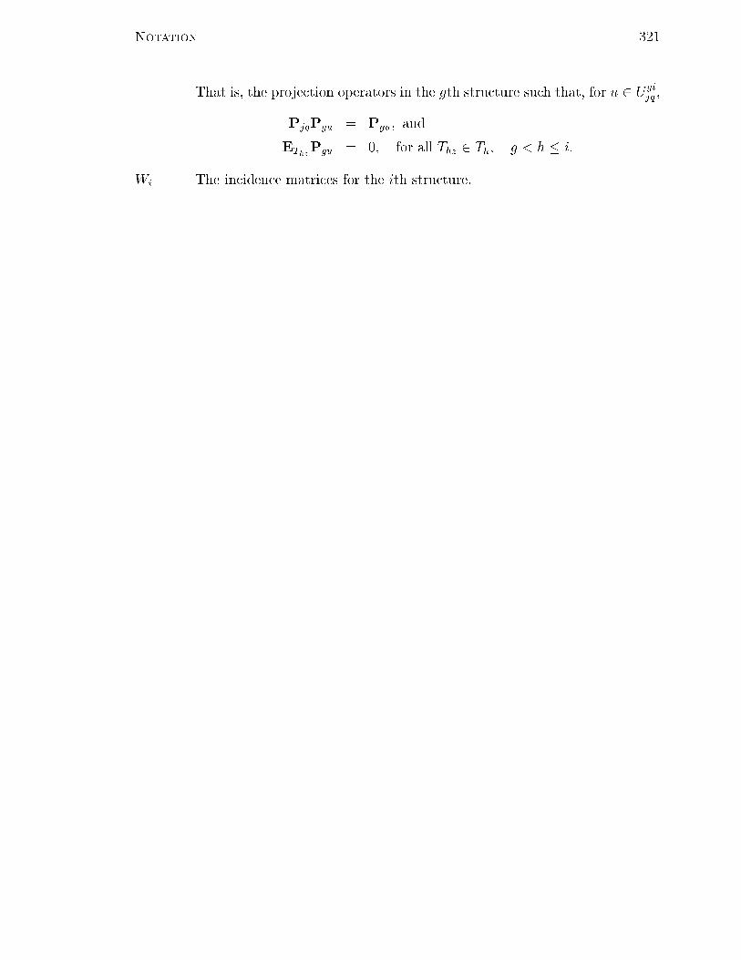
Notation 321
That is, the projection operators in the gth structure such that, for u 2 Ugijq ,
PjqPgu = Pgu; and
EThzPgu = 0; for all Thz 2 Th; g < h � i:
Wi The incidence matrices for the ith structure.

322
Bibliography
[Addelman, 1970] Addelman, S. (1970). Variability of treatments and experimental
units in the design and analysis of experiments. Journal of the American Statistical
Association, 65:1095{1108.
[Aigner, 1979] Aigner, M. (1979). Combinatorial Theory. Springer-Verlag, New York.
[Airy, 1861] Airy, G. B. (1861). On the Algebraical and Numerical Theory of Errors
of Observations and the Combination of Observations. Macmillan, London.
[Aitken, 1934] Aitken, A. C. (1934). On least squares and linear combination of
observations. Proceedings of the Royal Society of Edinburgh, Section A, 55:42{47.
[Aitkin, 1978] Aitkin, M. A. (1978). The analysis of unbalanced classi�cations (with
discussion). Journal of the Royal Statistical Society, Series A, 141:195{223.
[Allan and Wishart, 1930] Allan, F. E. and Wishart, J. (1930). A method of esti-
mating the yield of a missing plot in experimental work. Journal of Agricultural
Science, 20:399{406.
[Alvey et al., 1977] Alvey, N. G., Ban�eld, C. F., Baxter, R. I., Gower, J. C.,
Krzanowski, W. J., Lane, P. W., Leech, P. K., Nelder, J. A., Payne, R. W., Phelps,
K. M., Rogers, C. E., Ross, G. J. S., Simpson, H. R., Todd, A. D., Wedderburn,
R. W. C., and Wilkinson, G. N. (1977). Genstat Reference Manual. Statistics
Department, Rothamsted Experimental Station, Harpenden.
[Anderson, 1979] Anderson, R. D. (1979). On the history of variance component
estimation. In van Vleck, L. D. and Searle, S. R., editors, Variance Components
and Animal Breeding, pages 19{42. Cornell University Press, Ithaca, New York.

Bibliography 323
[Anderson and Bancroft, 1952] Anderson, R. L. and Bancroft, T. A. (1952). Statisti-
cal Theory in Research. McGraw-Hill, New York.
[Anderson, 1948] Anderson, T. W. (1948). On the theory of testing serial correlation.
Skandinavisk Aktuarietidskrift, 31:88{116.
[Anderson, 1970] Anderson, V. L. (1970). Restriction error for linear models (an aid
to develop models for designed experiments). Biometrics, 26:255{268.
[Anderson and Maclean, 1974] Anderson, V. L. and Maclean, R. A. (1974). Restric-
tion errors: Another dimension in teaching experimental statistics. The American
Statistician, 28:145{152.
[Anscombe, 1948] Anscombe, F. J. (1948). Contribution to the discussion of a paper
by Mr Champernowne. Journal of the Royal Statistical Society, Series B, 10:239.
[Appelbaum and Cramer, 1974] Appelbaum, M. I. and Cramer, E. M. (1974). Some
problems in the nonorthogonal analysis of variance. Psychological Bulletin, 81:335{
343.
[Bailey, 1981] Bailey, R. A. (1981). Distributive block structures and their automor-
phisms. In McAvaney, K., editor, Combinatorial Mathematics VIII: Proceedings of
the Eighth Australian Conference On Combinatorial Mathematics, Lecture Notes
in Mathematics 884, pages 115{124. Springer-Verlag, New York.
[Bailey, 1981a] Bailey, R. A. (1981a). A uni�ed approach to design of experiments.
Journal of the Royal Statistical Society, Series A, 144:214{223.
[Bailey, 1982a] Bailey, R. A. (1982a). Block structures for designed experiments. In
Wilson, R. J., editor, Applications of Combinatorics, pages 1{18. Shiva, Nantwich.
[Bailey, 1982b] Bailey, R. A. (1982b). Confounding. In Kotz, S. and Johnson, N. L.,
editors, Encyclopaedia of Statistical Sciences, volume 2, pages 128{134. John Wiley
& Sons, New York.
[Bailey, 1984] Bailey, R. A. (1984). Contribution to the discussion of a paper by
T. Tjur. International Statistical Review, 52:65{77.

Bibliography 324
[Bailey, 1985] Bailey, R. A. (1985). Nesting and crossing in design. In Kotz, S. and
Johnson, N. L., editors, Encyclopaedia of Statistical Sciences, volume 6, pages 181{
185. John Wiley & Sons, New York.
[Bailey, 1991] Bailey, R. A. (1991). Strata for randomized experiments. Journal of
the Royal Statistical Society, Series B, 53:27{78.
[Barnard, 1960] Barnard, G. A. (1960). Contribution to the discussion of a paper by
R. L. Plackett. Journal of the Royal Statistical Society, Series B, 22:214{215.
[Basu, 1980] Basu, D. (1980). Randomization analysis of experimental data: the
Fisher randomization test (with discussion). Journal of the American Statistical
Association, 75:575{595.
[Baxter and Wilkinson, 1970] Baxter, R. I. and Wilkinson, G. N. (1970). Genstat 4
user manual. Technical Report 6, CSIRO Division of Mathematical Statistics.
[Bennett and Franklin, 1954] Bennett, C. A. and Franklin, N. L. (1954). Statistical
Analysis in Chemistry and the Chemical Industry. John Wiley & Sons.
[Berge, 1971] Berge, C. (1971). Principles of Combinatorics. Academic Press, New
York.
[Blight and Pepper, 1984] Blight, G. W. and Pepper, P. M. (1984). Choosing the
experimental unit in grazing trials: Hobson's choice. unpublished manuscript.
[Bliss, 1967] Bliss, C. I. (1967). Statistics in Biology, volume I. McGraw-Hill, New
York.
[Bose, 1944] Bose, R. C. (1944). The fundamental theorem of linear estimation. (ab-
stract). In Proceedings of the 31st Indian Science Congress, pages 2{3.
[Box and Muller, 1959] Box, G. E. P. and Muller, M. E. (1959). Randomization and
least squares estimates. (abstract of paper presented in 1958). Journal of the Amer-
ican Statistical Association, 54:489.
[Brien, 1983] Brien, C. J. (1983). Analysis of variance tables based on experimental
structure. Biometrics, 39:51{59.

Bibliography 325
[Brien, 1989] Brien, C. J. (1989). A model comparison approach to linear models.
Utilitas Mathematica, 36:225{254.
[Brien et al., 1987] Brien, C. J., May, P., and Mayo, O. (1987). Analysis of judge
performance in wine-quality evaluations. Journal of Food Science, 52:1273{1279.
[Brien and Payne, 1989] Brien, C. J. and Payne, R. W. (1989). A note on the de-
scription of an experiment's structure. unpublished manuscript.
[Brien et al., 1984] Brien, C. J., Venables, W. N., James, A. T., and Mayo, O. (1984).
An analysis of correlation matrices: Equal correlations. Biometrika, 71:545{554.
[Brillinger et al., 1978] Brillinger, D. R., Jones, L. V., and Tukey, J. W. (1978). The
role of statistics in weather resources management. Technical report, Weather
Modi�cation Board Advisory Board. Report of the Statistical Task Force to the
Weather Modi�cation Board Advisory Board.
[Burdick and Herr, 1980] Burdick, D. S. and Herr, D. G. (1980). Counterexamples in
unbalanced two-way analysis of variance. Communications in Statistics { Theory
and Methods, A9:231{241.
[Chauvenet, 1863] Chauvenet, W. (1863). A Manual of Spherical and Practical As-
tronomy, volume I and II. Lippincott, Philadelphia.
[Clingele�er et al., 1977] Clingele�er, P. R., Trayford, R. S., May, P., and Brien, C. J.
(1977). Use of the starwheel sprayer for applying drying emulsion to Sultana grapes
to be dried on the trellis. Australian Journal of Experimental Agriculture and
Animal Husbandry, 17:871{880.
[Cochran, 1934] Cochran, W. G. (1934). The distribution of quadratic forms in a
normal system, with applications to the analysis of covariance. Proceedings of the
Cambridge Philosophical Society, 30:178{191.
[Cochran et al., 1941] Cochran, W. G., Autrey, K., and Cannon, C. (1941). A double
change-over design for dairy cattle feeding experiments. Journal of Dairy Science,
24:937{951.

Bibliography 326
[Cochran and Cox, 1957] Cochran, W. G. and Cox, G. M. (1957). Experimental De-
signs. John Wiley & Sons, New York, 2nd edition.
[Conni�e, 1976] Conni�e, D. (1976). A comparison of between and within herd vari-
ance in grazing experiments. Irish Journal of Agricultural Research, 15:39{46.
[Corbeil and Searle, 1976] Corbeil, R. R. and Searle, S. R. (1976). A comparison of
variance component estimators. Biometrics, 32:779{791.
[Corn�eld and Tukey, 1956] Corn�eld, J. and Tukey, J. W. (1956). Average values of
mean squares in factorials. Annals of Mathematical Statistics, 27:907{949.
[Corsten, 1976] Corsten, L. A. C. (1976). Canonical correlation in incomplete blocks.
In Ikeda, S., Hayakawa, T., Hudimoto, H., Okamota, M., Siotani, M., and Ya-
mamoto, S., editors, Essays in Probability and Statistics, chapter 10, pages 124{154.
Matsumoto, Japan.
[Cox, 1958] Cox, D. R. (1958). The interpretation of the e�ects of non-additivity in
the Latin square. Biometrika, 45:69{73.
[Cox, 1984] Cox, D. R. (1984). Interaction. International Statistical Review, 52:1{31.
[Cox and Hinkley, 1979] Cox, D. R. and Hinkley, D. V. (1979). Theoretical Statistics.
Chapman and Hall, London.
[Cox and Snell, 1981] Cox, D. R. and Snell, E. J. (1981). Applied Statistics. Chapman
and Hall, London.
[Crump, 1946] Crump, S. L. (1946). The estimation of variance components in the
analysis of variance. Biometrics Bulletin, 2:7{11.
[Crump, 1951] Crump, S. L. (1951). The present status of variance component anal-
ysis. Biometrics, 7:1{16.
[Curnow, 1959] Curnow, R. N. (1959). The analysis of a two phase experiment. Bio-
metrics, 15:60{73.
[Daniels, 1939] Daniels, H. E. (1939). The estimation of components of variance.
Journal of the Royal Statistical Society, Supplement, 6:186{197.

Bibliography 327
[Darroch, 1984] Darroch, J. N. (1984). Contribution to the discussion of a paper by
D. R. Cox. International Statistical Review, 52:26{27.
[Easterling, 1975] Easterling, R. G. (1975). Randomization and statistical inference.
Communications in Statistics, 4:723{735.
[Eden and Yates, 1933] Eden, T. and Yates, F. (1933). On the validity of Fisher's
Z�test when applied to an actual sample. Journal of Agricultural Science, 23:6{
16.
[Eisenhart, 1947] Eisenhart, C. (1947). The assumptions underlying the analysis of
variance. Biometrics, 3:1{21.
[Eisenhart, 1964] Eisenhart, C. (1964). The meaning of \least" in least squares. Jour-
nal of the Washington Academy of Sciences, 54:24{33.
[Elston and Bush, 1964] Elston, R. C. and Bush, N. (1964). The hypotheses that can
be tested when there are interactions in an analysis of variance model. Biometrics,
20:681{698.
[Ewart et al., 1985] Ewart, A. J. E., Brien, C. J., Soderlund, R., and Smart, R. E.
(1985). The e�ects of light pruning, irrigation and improved soil management on
wine quality of the vitis vinifera cv. Riesling. Vitis, 25:209{217.
[Federer, 1955] Federer, W. T. (1955). Experimental Design, Theory and Application.
Macmillan, New York.
[Federer, 1975] Federer, W. T. (1975). The misunderstood split plot. In Gupta, R. P.,
editor, Applied Statistics. North Holland, Amsterdam.
[Fisher, 1918] Fisher, R. A. (1918). The correlation between relatives on the suppo-
sition of Mendelian inheritance. Transactions of the Royal Society of Edinburgh,
52:388{433. Reprinted in Bennett, J. H., editor, (1971) Collected Papers of R. A.
Fisher., volume 1, pages 134-168. University of Adelaide, Adelaide.
[Fisher, 1925] Fisher, R. A. (1925). Statistical Methods for Research Workers. Oliver
and Boyd, Edinburgh, 1st edition.

Bibliography 328
[Fisher, 1935a] Fisher, R. A. (1935a). Contribution to the discussion of a paper by
F. Yates. Journal of the Royal Statistical Society, Supplement, 2:229{231. Incom-
plete extract in Bennett, J. H., editor, (1973) Collected Papers of R. A. Fisher.,
volume 3, pages 332-333. University of Adelaide, Adelaide.
[Fisher, 1935b] Fisher, R. A. (1935b). The Design of Experiments. Oliver and Boyd,
Edinburgh, 1st edition.
[Fisher, 1956] Fisher, R. A. (1956). Statistical Methods and Scienti�c Inference.
Oliver and Boyd, Edinburgh, 1st edition.
[Fisher, 1966] Fisher, R. A. (1966). The Design of Experiments. Oliver and Boyd,
Edinburgh, 8th edition.
[Fisher, 1970] Fisher, R. A. (1970). Statistical Methods for Research Workers. Oliver
and Boyd, Edinburgh, 14th edition.
[Fisher and Mackenzie, 1923] Fisher, R. A. and Mackenzie, W. A. (1923). Studies in
crop variation. II. The manurial response of di�erent potato varieties. Journal of
Agricultural Science Cambridge, 13:311{320. Reprinted in Bennett, J. H., editor,
(1971) Collected Papers of R. A. Fisher., volume 1, pages 469-478. University of
Adelaide, Adelaide.
[Free, 1977] Free, S. M. (1977). The consultant's forum: Designing nutrition studies
with litters. Biometrics, 33:561{563.
[Goldman and Zelen, 1964] Goldman, A. J. and Zelen, M. (1964). Weak generalized
inverses and minimum variance linear unbiased estimation. Journal of Research of
the National Bureau of Standards, Section B., 68b:151{172.
[Goodnight, 1980] Goodnight, J. H. (1980). Tests of hypotheses in �xed e�ects linear
models. Communications in Statistics { Theory and Methods, A9:167{180.
[Gossett, 1923] Gossett, W. S. (1923). On testing varieties of cereals. Biometrika,
15:271{293.
[Gr�atzer, 1971] Gr�atzer, G. (1971). Lattice Theory: First Concepts and Distributive
Lattices. Freeman, San Francisco.

Bibliography 329
[Graybill, 1961] Graybill, F. A. (1961). An Introduction to Linear Statistical Models,
volume 1. McGraw Hill, New York.
[Graybill, 1976] Graybill, F. A. (1976). Theory and Application of the Linear Model.
Duxbury Press, Massachusetts.
[Grenander, 1954] Grenander, U. (1954). On the estimation of the regression co-
eÆcients in the case of an auto-correlated disturbance. Annals of Mathematical
Statistics, 25:252{272.
[Grenander and Rosenblatt, 1957] Grenander, U. and Rosenblatt, M. (1957). Statis-
tical Analysis of Stationary Time Series. John Wiley & Sons, New York.
[Haberman, 1975] Haberman, S. J. (1975). Direct products and linear models for
complete factorial tables. Annals of Statistics, 3:314{333.
[Hale and Brien, 1978] Hale, C. R. and Brien, C. J. (1978). In uence of Salt Creek
rootstock on composition and quality of Shiraz grapes and wine. Vitis, 17:139{146.
[Harter, 1961] Harter, H. L. (1961). On the analysis of split-plot experiments. Bio-
metrics, 17:144{149.
[Harter, 1974] Harter, H. L. (1974). The method of least squares and some alterna-
tives. International Statistical Review, 42:147{174.
[Hartley and Rao, 1967] Hartley, H. O. and Rao, J. N. K. (1967). Maximum likelihood
estimation for the mixed analyses of variance model. Biometrika, 54:93{108.
[Harville, 1975] Harville, D. A. (1975). Experimental randomization: Who needs it?
The American Statistician, 29:27{31.
[Harville, 1977] Harville, D. A. (1977). Maximum-likelihood approaches to variance
component estimation and to related problems. Journal of the American Statistical
Association, 72:320{340.
[Harville, 1978] Harville, D. A. (1978). Alternative formulations and procedures for
the two-way mixed model. Biometrics, 34:441{454.
[Henderson, 1953] Henderson, C. R. (1953). Estimation of variance and covariance
components. Biometrics, 9:226{252.

Bibliography 330
[Hinkley, 1980] Hinkley, D. V. (1980). Contribution to the discussion of a paper by
D. Basu. Journal of the American Statistical Association, 75:582{584.
[Hocking and Kutner, 1975] Hocking, R. R. and Kutner, M. H. (1975). Some analyt-
ical and numerical comparisons of estimators for the mixed aov model. Biometrics,
31:19{28.
[Hocking and Speed, 1975] Hocking, R. R. and Speed, F. M. (1975). A full rank anal-
ysis of some linear model problems. Journal of the American Statistical Association,
70:706{712.
[Hocking et al., 1980] Hocking, R. R., Speed, F. M., and Coleman, A. T. (1980).
Hypotheses to be tested with unbalanced data. Communications in Statistics {
Theory and Methods, A9:117{129.
[Houtman and Speed, 1983] Houtman, A. M. and Speed, T. P. (1983). Balance in de-
signed experiments with orthogonal block structure. Annals of Statistics, 11:1069{
1085.
[Huynh and Feldt, 1970] Huynh, H. and Feldt, L. S. (1970). Conditions under which
mean square ratios in repeated measurements designs have exact F�distribution.
Journal of the American Statistical Association, 65:1582{1589.
[Irwin, 1931] Irwin, J. O. (1931). Mathematical theorems involved in the analysis of
variance. Journal of the Royal Statistical Society, 94:284{300.
[Irwin, 1934] Irwin, J. O. (1934). On the independence of the constituent items in the
analysis of variance. Journal of the Royal Statistical Society, Supplement, 1:236{
251.
[Irwin, 1960] Irwin, J. O. (1960). Contribution to the discussion of a paper by
R. L. Plackett. Journal of the Royal Statistical Society, Series B, 22:212{213.
[Jackson, 1939] Jackson, R. W. B. (1939). Reliability of mental tests. British Journal
of Psychology, 29:267{287.
[James, 1957] James, A. T. (1957). The relationship algebra of an experimental de-
sign. Annals of Mathematical Statistics, 28:993{1002.

Bibliography 331
[James, 1982] James, A. T. (1982). Analyses of variance determined by symmetry
and combinatorial properties of zonal polynomials. In Kallianpur, G., Krishnaiah,
P. R., and Gosh, J. K., editors, Statistics and Probability: Essays in Honour of
C. R. Rao, pages 329{341. North Holland, Amsterdam.
[James and Wilkinson, 1971] James, A. T. and Wilkinson, G. N. (1971). Factoriza-
tion of the residual operator and canonical decomposition of nonorthogonal factors
in the analysis of variance. Biometrika, 58:279{294.
[John and Quenouille, 1977] John, J. A. and Quenouille, M. H. (1977). Experiments:
Design and Analysis. GriÆn, London, 2nd edition.
[Kempthorne, 1952] Kempthorne, O. (1952). The Design and Analysis of Experi-
ments. John Wiley & Sons, New York.
[Kempthorne, 1955] Kempthorne, O. (1955). The randomization theory of experi-
mental inference. Journal of the American Statistical Association, 50:940{967.
[Kempthorne, 1966] Kempthorne, O. (1966). Some aspects of experimental inference.
Journal of the American Statistical Association, 61:11{34.
[Kempthorne, 1975a] Kempthorne, O. (1975a). Fixed and mixed models in the anal-
ysis of variance. Biometrics, 31:473{486.
[Kempthorne, 1975b] Kempthorne, O. (1975b). Inference from experiments and ran-
domization. In Srivastava, J. N., editor, A Survey of Statistical Design and Linear
Models, pages 303{331. North Holland, Amsterdam.
[Kempthorne, 1976a] Kempthorne, O. (1976a). The analysis of variance and facto-
rial design. In Owen, D. B., editor, On the History of Statistics and Probability,
volume 17, pages 29{54. Marcel-Dekker, New York.
[Kempthorne, 1976b] Kempthorne, O. (1976b). Best linear unbiased estimation with
arbitrary variance matrix. In Ikeda, S., Hayakawa, T., Hudimoto, H., Okamota,
M., Siotani, M., and Yamamoto, S., editors, Essays in Probability and Statistics,
chapter 14, pages 203{225. Matsumoto, Japan.

Bibliography 332
[Kempthorne, 1977] Kempthorne, O. (1977). Why randomize? Journal of Statistical
Planning and Inference, 1:1{25.
[Kempthorne, 1980] Kempthorne, O. (1980). Contribution to the discussion of a pa-
per by D. Basu. Journal of the American Statistical Association, 75:584{587.
[Kempthorne and Folks, 1971] Kempthorne, O. and Folks, J. L. (1971). Probability,
Statistics, and Data Analysis. Iowa State University Press, Ames, Iowa.
[Kendall and Buckland, 1960] Kendall, M. G. and Buckland, W. R. (1960). A Dic-
tionary of Statistical Terms. Oliver and Boyd, Edinburgh, 2nd edition.
[Khuri, 1982] Khuri, A. I. (1982). Direct products: a powerful tool for the analysis of
balanced data. Communication in Statistics { Theory and Methods, 11:2903{2920.
[Koch et al., 1988] Koch, G. G., Elasho�, J. D., and Amara, I. A. (1988). Repeated
measurements { design and analysis. In Kotz, S. and Johnson, N. L., editors,
Encyclopaedia of Statistical Sciences, volume 8, pages 46{73. John Wiley & Sons,
New York.
[Kruskal, 1968] Kruskal, W. H. (1968). When are least squares and Gauss-Markov es-
timators identical? A coordinate-free approach. Annals of Mathematical Statistics,
39:70{75.
[Kunert, 1983] Kunert, J. (1983). Optimal design and re�nement of the linear model
with applications to repeated measurements designs. The Annals of Statistics,
11:247{257.
[Kurkjian and Zelen, 1963] Kurkjian, B. and Zelen, M. (1963). Applications of the
calculus of factorial arrangements. I. Block and direct product designs. Biometrika,
50:63{73.
[Lindley, 1980] Lindley, D. V. (1980). Contribution to the discussion of a paper by
D. Basu. Journal of the American Statistical Association, 75:589{590.
[Magness and McGuire, 1962] Magness, T. A. and McGuire, J. B. (1962). Compar-
ison of least squares and minimum variance estimates of regression parameters.
Annals of Mathematical Statistics, 33:462{470.

Bibliography 333
[McCarthy, 1939] McCarthy, M. D. (1939). On the application of the Z�test to
randomized blocks. Annals of Mathematical Statistics, 10:337{359.
[McCullagh and Nelder, 1983] McCullagh, P. and Nelder, J. A. (1983). Generalized
Linear Models. Chapman and Hall, London.
[McIntyre, 1955] McIntyre, G. A. (1955). Design and analysis of two phase experi-
ments. Biometrics, 11:324{334.
[McIntyre, 1956] McIntyre, G. A. (1956). Query 123. Biometrics, 12:527{532.
[Mead and Curnow, 1983] Mead, R. and Curnow, R. N. (1983). Statistical Methods
in Agriculture and Experimental Biology. Chapman and Hall, London.
[Miller, 1977] Miller, J. J. (1977). Asymptotic properties of maximum likelihood
estimates in the mixed model of the analysis of variance. Annals of Statistics,
5:746{762.
[Millman and Glass, 1967] Millman, J. and Glass, G. V. (1967). Rules of thumb for
writing the anova table. Journal of Educational Measurement, 4:41{51.
[Mitra and Moore, 1973] Mitra, S. K. and Moore, B. J. (1973). Gauss-Markov esti-
mation with an incorrect dispersion matrix. Sankhya, Series A, 35:139{152.
[Mitra and Rao, 1968] Mitra, S. K. and Rao, C. R. (1968). Some results in estimation
and tests of linear hypotheses under the Gauss-Markov model. Sankhya, Series A,
30:281{290.
[Mitra and Rao, 1969] Mitra, S. K. and Rao, C. R. (1969). Conditions for optimality
and validity of simple least squares theory. Annals of Mathematical Statistics,
40:1617{1624.
[Morley Jones, 1959] Morley Jones, R. (1959). A property of incomplete blocks. Jour-
nal of the Royal Statistical Society, Series B, 21:172{179.
[Muller and Watson, 1959] Muller, M. E. and Watson, G. S. (1959). Randomization
and linear least squares estimation. Technical Report 32, Statistical Techniques
Research Group, Princeton University.

Bibliography 334
[Nelder, 1965a] Nelder, J. A. (1965a). The analysis of randomized experiments with
orthogonal block structure. I. Block structure and the null analysis of variance.
Proceedings of the Royal Society, Series A, 283:147{161.
[Nelder, 1965b] Nelder, J. A. (1965b). The analysis of randomized experiments with
orthogonal block structure. II. Treatment structure and the general analysis of
variance. Proceedings of the Royal Society, Series A, 283:162{178.
[Nelder, 1968] Nelder, J. A. (1968). The combination of information in generally
balanced designs. Journal of the Royal Statistical Society, Series B, 30:303{311.
[Nelder, 1977] Nelder, J. A. (1977). A reformulation of linear models (with discus-
sion). Journal of the Royal Statistical Society, Series A, 140:48{76.
[Nelder, 1982] Nelder, J. A. (1982). Linear models and non-orthogonal data. Utilitas
Mathematica, 21A:141{152.
[Neyman, 1923] Neyman, J. (1923). Sur les applications de la th�eorie des probabilit�es
aux experi�ences agricols. Essay des principes. Roczniki Nauk Rolniczych, 10:1{51.
[Neyman, 1934] Neyman, J. (1934). On two di�erent aspects of the representative
method. Journal of the Royal Statistical Society, 97:558{625.
[Neyman and Kolodzieczyk, 1935] Neyman, J. with the cooperation of Iwaskiewicz,
K. and Kolodzieczyk, S. (1935). Statistical problems in agricultural experimentation
(with discussion). Journal of the Royal Statistical Society, Supplement, 2:107{180.
[Ogawa, 1980] Ogawa, J. (1980). Experimental randomization in statistical inference.
In Matusita, K., editor, Recent Developments in Statistical Inference and Data
Analysis, pages 237{246. North Holland, Amsterdam.
[Payne and Dixon, 1983] Payne, R. W. and Dixon, T. J. (1983). The analysis of
experiments with repeated measures. Genstat Newsletter, 11:10{22.
[Payne et al., 1987] Payne, R. W., Lane, P. W., Ainsley, A. E., Bicknell, K. E., Digby,
P. G. N., Harding, S. A., Leech, P. K., Simpson, H. R., Todd, A. D., Verrier, P. J.,
White, R. P., Gower, J. C., Tunnicli�e Wilson, G., and Paterson, L. J. (1987).
Genstat 5 Reference Manual. Oxford University Press, Oxford.

Bibliography 335
[Payne and Wilkinson, 1977] Payne, R. W. and Wilkinson, G. N. (1977). A general
algorithm for analysis of variance. Applied Statistics, 26:251{260.
[Pearce et al., 1974] Pearce, S. C., Cali�nski, T., and Marshall, T. F. D. (1974). The
basic contrasts of an experimental design with special reference to the analysis of
data. Biometrika, 61:449{460.
[Pitman, 1938] Pitman, E. J. G. (1938). Signi�cance tests which may be applied to
samples from any population. Biometrika, 29:322{335.
[Plackett, 1960] Plackett, R. L. (1960). Models in analysis of variance (with discus-
sion). Journal of the Royal Statistical Society Series B, 22:195{217.
[Plackett, 1972] Plackett, R. L. (1972). Studies in the history of probability and
statistics. XXIX. The discovery of the method of least squares. Biometrika, 59:239{
251.
[Preece, 1982] Preece, D. A. (1982). The design and analysis of experiments: what
has gone wrong? Utilitas Mathematica, 21A:201{244.
[Preece et al., 1978] Preece, D. A., Bailey, R. A., and Patterson, H. D. (1978). A ran-
domization problem in forming designs with superimposed treatments. Australian
Journal of Statistics, 20:111{125.
[Rao, 1959] Rao, C. R. (1959). Expected values of mean squares in the analysis
of incomplete block experiments and some comments based on them. Sankhya,
21:327{336.
[Rao, 1967] Rao, C. R. (1967). Least squares theory using an estimated dispersion
matrix and its application to measurement of signals. In le Cam, L. M. and Neyman,
J., editors, Proceedings of the Fifth Berkeley Symposium on Mathematical Statistics
and Probability, pages 355{372, Berkeley, California. University of California Press.
[Rao, 1968] Rao, C. R. (1968). A note on a previous lemma in the theory of least
squares and some further results. Sankhya, Series A, 30:259{266.
[Rao, 1971] Rao, C. R. (1971). Uni�ed theory of linear estimation. Sankhya, Series
A, 33:371{394.

Bibliography 336
[Rao, 1972] Rao, C. R. (1972). Some recent results in linear estimation. Sankhya,
Series B, 34:369{378.
[Rao, 1973] Rao, C. R. (1973). Uni�ed theory of least squares. Communications in
Statistics, 1:1{8.
[Rao, 1973b] Rao, C. R. (1973b). Linear Statistical Inference and its Applications.
John Wiley & Sons, New York, 2nd edition.
[Rao, 1974] Rao, C. R. (1974). Projectors, generalized inverses and the BLUE's.
Journal of the Royal Statistical Society Series B, 36:442{448.
[Rao, 1978] Rao, C. R. (1978). Least squares theory for possibly singular models.
Canadian Journal of Statistics, 6:19{23.
[Rao and Mitra, 1971] Rao, C. R. and Mitra, S. K. (1971). Further contributions to
the theory of generalized inverse of matrices and its applications. Sankhya, Series
A, 33:289{300.
[Rao and Yanai, 1979] Rao, C. R. and Yanai, H. (1979). General de�nition and de-
composition of projectors and some applications to statistical problems. Journal of
Statistical Planning and Inference, 3:1{17.
[Rota, 1964] Rota, G.-C. (1964). On the foundations of combinatorial theory. I. The-
ory of M�obius functions. Zeitschrift f�ur Wahrscheinlichkeitstheorie und verwandte
Gebiete, 2:340{368.
[Rouanet and L�epine, 1970] Rouanet, H. and L�epine, D. (1970). Comparison between
treatments in a repeated-measurement design: ANOVA and multivariate methods.
The British Journal of Mathematical and Statistical Psychology, 23:147{163.
[Rubin, 1980] Rubin, D. B. (1980). Discussion of randomization analysis of experi-
mental data: the Fisher randomization test by D. Basu. Journal of the American
Statistical Association, 75:591{593.
[Sahai, 1979] Sahai, H. (1979). A bibliography on variance components. International
Statistical Review, 47:177{222.

Bibliography 337
[Satterthwaite, 1946] Satterthwaite, F. E. (1946). An approximate distribution of
estimates of variance components. Biometrics, 2:110{114.
[Sche��e, 1956] Sche��e, H. (1956). Alternative models for the analysis of variance.
Annals of Mathematical Statistics, 27:251{271.
[Sche��e, 1959] Sche��e, H. (1959). The Analysis of Variance. John Wiley & Sons,
New York.
[Schultz Jr., 1955] Schultz Jr., E. F. (1955). Rules of thumb for determining expec-
tations of mean squares in analysis of variance. Biometrics, 11:123{135.
[Seal, 1967] Seal, H. L. (1967). Studies in the history of probability and statistics.
XV. The historical development of the Gauss linear model. Biometrika, 54:1{24.
[Searle, 1968] Searle, S. R. (1968). Another look at Henderson's methods of estimating
variance components (with discussion). Biometrics, 24:749{778.
[Searle, 1971] Searle, S. R. (1971). Topics in variance component estimation. Bio-
metrics, 27:1{76.
[Searle, 1971b] Searle, S. R. (1971b). Linear Models. John Wiley & Sons, New York.
[Searle, 1974] Searle, S. R. (1974). Prediction, mixed models, and variance compo-
nents. In Proschan, F. and Ser ing, R. J., editors, Reliability and Biometry, pages
229{266. Society for Industrial and Applied Mathematics, Philadelphia.
[Searle, 1979a] Searle, S. R. (1979a). Notes on variance component estimation: a de-
tailed account of maximum likelihood and kindred methodology. Technical Report
Bu-673-M, Biometrics Unit, Cornell University, Ithaca, New York.
[Searle, 1979b] Searle, S. R. (1979b). Maximum likelihood and minimum variance
estimation of variance components. In van Vleck, L. D. and Searle, S. R., editors,
Variance Components and Animal Breeding, pages 59{68. Cornell University Press,
Ithaca, New York.
[Searle and Henderson, 1979] Searle, S. R. and Henderson, H. V. (1979). Dispersion
matrices for variance components models. Journal of the American Statistical As-
sociation, 74:465{470.

Bibliography 338
[Searle et al., 1981] Searle, S. R., Speed, F. M., and Henderson, H. V. (1981). Some
computational and model equivalences in analyses of variance of unequal-subclass-
numbers data. The American Statistician, 35:16{33.
[Seely, 1970] Seely, J. (1970). Linear spaces and unbiased estimation. Annals of
Mathematical Statistics, 41:1725{1734.
[Seely and Zyskind, 1971] Seely, J. and Zyskind, G. (1971). Linear spaces and mini-
mum variance unbiased estimation. Annals of Mathematical Statistics, 42:691{703.
[Sheynin, 1978] Sheynin, O. B. (1978). C. F. Gauss and the theory of errors. Archives
of History of Exact Science, 20:21{72.
[Smith and Hocking, 1978] Smith, D. W. and Hocking, R. R. (1978). Maximum like-
lihood analysis of the mixed model: the balanced case. Communication in Statistics
{ Theory and Methods, A7:1253{1266.
[Smith and Murray, 1984] Smith, D. W. and Murray, L. W. (1984). An alternative to
Eisenhart's model II and mixed model in the case of negative variance estimates.
Journal of the American Statistical Association, 79:145{151.
[Smith, 1955] Smith, H. F. (1955). Variance components, �nite populations, and
experimental inference. Mimeo Series 135, University of North Carolina Institute
of Statistics.
[Snedecor and Cochran, 1980] Snedecor, G. W. and Cochran, W. G. (1980). Statisti-
cal Methods. Iowa State University Press, Ames, Iowa, 7th edition.
[Speed and Hocking, 1976] Speed, F. M. and Hocking, R. R. (1976). The use of the
R()�notation with unbalanced data. The American Statistician, 30:30{33.
[Speed et al., 1978] Speed, F. M., Hocking, R. R., and Hackney, O. P. (1978). Meth-
ods of analysis of linear models with unbalanced data. Journal of the American
Statistical Association, 73:105{112.
[Speed, 1986] Speed, T. P. (1986). ANOVA models with random e�ects: an approach
via symmetry. In Gani, J. and Priestley, M. B., editors, Essays in Time Series

Bibliography 339
and Allied Processes: Papers in Honour of E. J. Hannan, pages 355{368. Applied
Probability Trust, SheÆeld.
[Speed and Bailey, 1982] Speed, T. P. and Bailey, R. A. (1982). On a class of associa-
tion schemes derived from lattices of equivalence relations. In Schultz, P., Praeger,
C. E., and Sullivan, R. P., editors, Algebraic Structures and Applications, pages
55{74. Marcel-Dekker, New York.
[Speed and Bailey, 1987] Speed, T. P. and Bailey, R. A. (1987). Factorial dispersion
models. International Statistical Review, 55:251{277.
[Steel and Torrie, 1980] Steel, R. G. D. and Torrie, J. H. (1980). Principles and
Procedures of Statistics. McGraw-Hill, New York, 2nd edition.
[Steinhorst, 1982] Steinhorst, R. K. (1982). Resolving current controversies in analysis
of variance. The American Statistician, 36:138{139.
[Szatrowski, 1980] Szatrowski, T. H. (1980). Necessary and suÆcient conditions for
explicit solutions in the multivariate normal estimations problem for patterned
means and covariances. Annals of Statistics, 8:802{810.
[Szatrowski and Miller, 1980] Szatrowski, T. H. and Miller, J. J. (1980). Explicit max-
imum likelihood estimates from balanced data in the mixed model of the analysis
of variance. Annals of Statistics, 8:811{819.
[Thomas, 1968] Thomas, D. H. (1968). When do minimum variance estimators coin-
cide? (abstract). Annals of Mathematical Statistics, 39:1365.
[Tippett, 1929] Tippett, L. H. C. (1929). Statistical methods in textile research. The
analysis of complex variations. Shirley Institute Memoirs, 8:175{196.
[Tippett, 1931] Tippett, L. H. C. (1931). The Methods of Statistics. Williams and
Norgate, London.
[Tjur, 1984] Tjur, T. (1984). Analysis of variance models in orthogonal designs. In-
ternational Statistical Review, 52:33{81.
[Tukey, 1977] Tukey, J. W. (1977). Contribution to the discussion of a paper by
J. A. Nelder. Journal of the Royal Statistical Society, Series A, 140:72.

Bibliography 340
[Urquhart and Weeks, 1978] Urquhart, N. S. and Weeks, D. L. (1978). Linear models
in messy data: some problems and alternatives. Biometrics, 34:696{705.
[Urquhart et al., 1973] Urquhart, N. S., Weeks, D. L., and Henderson, C. R. (1973).
Estimation associated with linear models: a revisitation. Communications in Statis-
tics, 1:303{330.
[Watson, 1955] Watson, G. S. (1955). Serial correlation in regression analysis, I.
Biometrika, 42:327{341.
[Watson, 1967] Watson, G. S. (1967). Linear least squares regression. Annals of
Mathematical Statistics, 38:1679{1699.
[Watson, 1972] Watson, G. S. (1972). Prediction and the eÆciency of least squares.
Biometrika, 59:91{98.
[Welch, 1937] Welch, B. L. (1937). On the Z�test in randomized blocks and Latin
squares. Biometrika, 29:21{52.
[White, 1975] White, R. F. (1975). Randomization and the analysis of variance.
Biometrics, 31:552{572.
[Whittaker, 1965] Whittaker, I. A. M. (1965). Factors A�ecting the Intake of Herbage
by the Grazing Animal. PhD thesis, Waite Agricultural Research Institute, the
University of Adelaide, Adelaide, South Australia.
[Wilk, 1955] Wilk, M. B. (1955). The randomization analysis of a generalized ran-
domized block design. Biometrika, 42:70{79.
[Wilk and Kempthorne, 1955] Wilk, M. B. and Kempthorne, O. (1955). Fixed,
mixed, and random models. Journal of the American Statistical Association,
50:1144{1167.
[Wilk and Kempthorne, 1956] Wilk, M. B. and Kempthorne, O. (1956). Some aspects
of the analysis of factorial experiments in a completely randomized design. Annals
of Mathematical Statistics, 27:950{985.

Bibliography 341
[Wilk and Kempthorne, 1957] Wilk, M. B. and Kempthorne, O. (1957). Non-
additivities in the Latin square design. Journal of the American Statistical As-
sociation, 52:218{236.
[Wilkinson, 1970] Wilkinson, G. N. (1970). A general recursive procedure for analysis
of variance. Biometrika, 57:19{46.
[Wilkinson et al., 1983] Wilkinson, G. N., Eckert, S. R., Hancock, T. W., and Mayo,
O. (1983). Nearest neighbour (NN) analysis of �eld experiments (with discussion).
Journal of the Royal Statistical Society, Series B, 45:151{211.
[Wilkinson and Rogers, 1973] Wilkinson, G. N. and Rogers, C. E. (1973). Symbolic
description of factorial models for analysis of variance. Applied Statistics, 22:392{
399.
[Winer, 1971] Winer, B. J. (1971). Statistical Principles in Experimental Designs.
McGraw-Hill, New York, 2nd edition.
[Wood et al., 1988] Wood, J. T., Williams, E. R., and Speed, T. P. (1988). Non-
orthogonal block structure in two-phase designs. Australian Journal of Statistics,
30A:225{237.
[Yates, 1933] Yates, F. (1933). The principles of orthogonality and confounding in
replicated experiments. Journal of Agricultural Science, 23:108{145. Reprinted
with additional author's note in Yates, F. (1970) Experimental Design: Selected
Papers. pages 1-40. GriÆn, London.
[Yates, 1934] Yates, F. (1934). The analysis of multiple classi�cations with unequal
numbers in the di�erent classes. Journal of the American Statistical Association,
29:51{66.
[Yates, 1936] Yates, F. (1936). A new method of arranging variety trials involving a
large number of varieties. Journal of Agricultural Science, 26:424{455. Reprinted
with additional author's note in Yates, F. (1970) Experimental Design: Selected
Papers. pages 147-180. GriÆn, London.
[Yates, 1965] Yates, F. (1965). A fresh look at the basic principles of the design and
analysis of experiments. In le Cam, L. M. and Neyman, J., editors, Proceedings of

Bibliography 342
the Fourth Berkeley Symposium on Mathematical Statistics and Probability, pages
777{790, Berkeley, California. University of California Press. Reprinted with ad-
ditional author's note in Yates, F. (1970) Experimental Design: Selected Papers.
pages 265-286. GriÆn, London.
[Yates, 1970] Yates, F. (1970). Author's note on �xed and random e�ects models. In
Experimental Design: Selected Papers, pages 281{286. GriÆn, London.
[Yates, 1975] Yates, F. (1975). The early history of experimental design. In Srivastava,
J. N., editor, A Survey of Statistical Design and Linear Models, pages 581{592.
North Holland, Amsterdam.
[Yates, 1977] Yates, F. (1977). Contribution to the discussion of a paper by
J. A. Nelder. Journal of the Royal Statistical Society, Series A, 140:67{68.
[Yates and Cochran, 1938] Yates, F. and Cochran, W. G. (1938). The analysis of
groups of experiments. Journal of Agricultural Science, 28:556{580. Reprinted
with additional author's note in Yates, F. (1970) Experimental Design: Selected
Papers. pages 119-145. GriÆn, London.
[Zelen and Federer, 1964] Zelen, M. and Federer, W. T. (1964). Application of the
calculus for factorial arrangements, II. Two-way elimination of heterogeneity. An-
nals of Mathematical Statistics, 35:658{672.
[Zyskind, 1962a] Zyskind, G. (1962a). On conditions for equality of best and sim-
ple linear least squares estimators. (abstract). Annals of Mathematical Statistics,
33:1502{1503.
[Zyskind, 1962b] Zyskind, G. (1962b). On structure, relation, �, and expectation of
means squares. Sankhya Series A, 24:115{148.
[Zyskind, 1963] Zyskind, G. (1963). Some consequences of randomization in a general-
ization of the balanced incomplete block design. Annals of Mathematical Statistics,
34:1569{1581.
[Zyskind, 1967] Zyskind, G. (1967). On canonical forms, non-negative covariance
matrices and best and simple least squares linear estimators in linear models. Annals
of Mathematical Statistics, 38:1092{1109.

Bibliography 343
[Zyskind, 1975] Zyskind, G. (1975). Error structures, projections and conditional
inverses in linear model theory. In Srivastava, J. N., editor, A Survey of Statistical
Design and Linear Models, pages 647{663. North Holland, Amsterdam.
[Zyskind and Martin, 1969] Zyskind, G. and Martin, F. B. (1969). On best linear
estimation and a general Gauss-Markov theorem in linear models with arbitrary
nonnegative covariance structure. SIAM Journal of Applied Mathematics, 17:1190{
1202.

![Untitled-2 [] · FS 78 FS 68 , FOCUS ÉkJ ËFOCUS FS 78 FS 68 FS 68 , , , FS 68 Foundation FS 68 , FS 68 68 fi , FOCUS F-s 688 , , 68 , 688 FOCUS FS , FS 68 , , , 688 ,](https://static.documents.pub/doc/80x56/5b75f9b67f8b9a3b7e8b5e04/untitled-2-fs-78-fs-68-focus-ekj-efocus-fs-78-fs-68-fs-68-fs-68.jpg)


![Title 68 RCW - Washington State · 2016. 9. 23. · (2016 Ed.) [Title 68 RCW—page 1] Title 68 Title 68 68 CEMETERIES, MORGUES, AND HUMAN REMAINSCEMETERIES, MORGUES, AND HUMAN REMAINS](https://static.documents.pub/doc/80x56/60aab8bfaf00663cd7475042/title-68-rcw-washington-state-2016-9-23-2016-ed-title-68-rcwapage-1.jpg)


