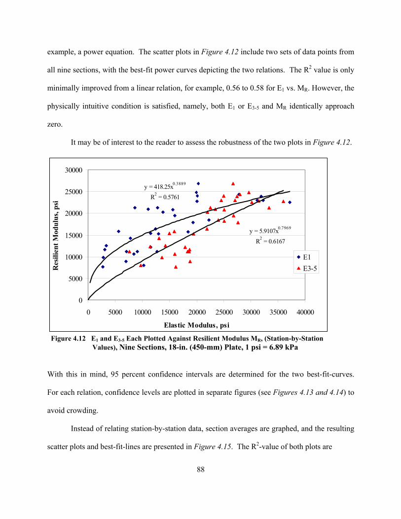
FALLING WEIGHT DEFLECTOMETER FOR ESTIMATING SUBGRADE RESILIENT MODULI FINAL REPORT by K.P. George Conducted by the DEPARTMENT OF CIVIL ENGINEERING UNIVERSITY OF MISSISSIPPI In cooperation with THE MISSISSIPPI DEPARTMENT OF TRANSPORTATION And U.S. DEPARTMENT OF TRANSPORTATION FEDERAL HIGHWAY ADMINISTRATION The University of Mississippi University, Mississippi October 2003
Transcript
FALLING WEIGHT DEFLECTOMETER FOR ESTIMATING SUBGRADE
RESILIENT MODULI
FINAL REPORT
by
K.P. George
Conducted by the
DEPARTMENT OF CIVIL ENGINEERING UNIVERSITY OF MISSISSIPPI
In cooperation with
THE MISSISSIPPI DEPARTMENT OF TRANSPORTATION
And
U.S. DEPARTMENT OF TRANSPORTATION FEDERAL HIGHWAY ADMINISTRATION
The University of Mississippi University, Mississippi
October 2003
ii
Technical Report Documentation Page
Form DOT F 1700.7 (8-72) Reproduction of completed page authorized
1.Report No. FHWA/MS-DOT-RD-03-153
2. Government Accession No.
3. Recipient’s Catalog No.
5. Report Date December 2003
4. Title and Subtitle Falling Weight Deflectometer for Estimating Subgrade Moduli
9. Performing Organization Name and Address University of Mississippi Department of Civil Engineering University, MS 38677 11. Contract or Grant No.
State Study 153 13. Type Report and Period Covered
January 2002 – December 31, 2003 Final Report
12. Sponsoring Agency Name and Address Mississippi Department of Transportation Research Division P.O. Box 1850 Jackson, MS 39215-1850
14. Sponsoring Agency Code
15. Supplementary Notes 16. Abstract Subgrade soil characterization expressed in terms of resilient modulus, MR, has become crucial for pavement design. For new pavement design, MR values are generally obtained by conducting repeated load triaxial tests on reconstituted/undisturbed cylindrical specimens, employing TP46 protocol. Because of the complexities encountered with the test, in situ tests would be desirable if reliable correlation can be established. In evaluating existing pavements for rehabilitation selection, subgrade characterization is even more complex. The focus of this study is to investigate the viability of Falling Weight Deflectometer (FWD) for direct testing of subgrade with the object of deriving resilient modulus, via a correlation between FWD modulus and MR. In support of this research, side-by-side Automated Dynamic Cone Penetrometer (ADCP) tests were also conducted. Ten as-built subgrade sections reflecting typical subgrade soil materials of Mississippi were selected and tested with FWD. Both fine- and coarse-grain soils were included in the program. Undisturbed samples were extracted using a Shelby tube and tested in a repeated load triaxial machine for MR, employing TP46 protocol. Other routine laboratory tests are conducted to determine physical properties, and, in turn, classify the soil being tested. Employing seven FWD sensor deflections, elastic moduli, E1 to E7, are calculated employing forward equations (assuming static half-space). E1 and E3-5 (average of E3, E4, and E5) are regressed against MR, advancing two models for MR prediction. Employing E1 and E3-5, two distinct resilient moduli are derived, with the lesser of the two serving as the design resilient modulus. A feature of the model is that both center sensor modulus and offset sensor moduli enter in the process, yielding a representative, but conservative, resilient modulus for design. Having been derived from multiple sensor moduli, this procedure promises to be a viable method for subgrade characterization, considering significant nonhomogenity expected of built-up subgrades. Also suggested is a short-cut procedure for predicting resilient modulus which employs an E3-5 section average for a low moduli range, that is, E1<9000 psi (62 MPa), and lesser of E1 and E3-5 for E1>9000 psi (62 MPa). An exclusive program, FWDSUBGRADE, is developed to analyze FWD deflection data from subgrade tests, extracting first sensor modulus E1, and average of three offset sensor moduli, E3-5, from which only design resilient modulus is derived. The program, in addition to calculating station-by-station resilient modulus, relying on what is known as “cumulative difference” technique, delineates homogenous units of the subgrade, outputting mean and standard deviation of the resilient modulus for each homogenous section. A graphical plot of resilient modulus of each station is another output of the program.
This report includes the results of a study titled “Falling Weight Deflectometer for
Estimating Subgrade Moduli”, conducted by the Department of Civil Engineering, The
University of Mississippi, in cooperation with the Mississippi Department of Transportation
(MDOT), and the U.S. Department of Transportation, Federal Highway Administration
(FHWA). Funding of this project by MDOT and FHWA is gratefully acknowledged.
The author wishes to thank Bill Barstis with MDOT’s Research Division for his efforts in
coordinating the overall work plan of the project. Johnny Hart of MDOT coordinated the
fieldwork, including FWD tests; Alan Hatch of MDOT conducted ADCP tests. Richard
Stubstad’s (ERES/ARA) assistance in the data analysis phase of this project is acknowledged.
Manil Bajracharya and Madan Gaddam were the key personnel from the University
conducting laboratory work and providing support in the field. The service of Sherra Jones in
preparing this report is gratefully acknowledged.
iv
ABSTRACT
Subgrade soil characterization expressed in terms of resilient modulus, MR, has become
crucial for pavement design. For new pavement design, MR values are generally obtained by
conducting repeated load triaxial tests on reconstituted/undisturbed cylindrical specimens,
employing TP46 protocol. Because of the complexities encountered with the test, in situ tests
would be desirable if reliable correlation can be established. In evaluating existing pavements
for rehabilitation selection, subgrade characterization is even more complex. The focus of this
study is to investigate the viability of Falling Weight Deflectometer (FWD) for direct testing of
subgrade with the object of deriving resilient modulus, via a correlation between FWD modulus
and MR. In support of this research, side-by-side Automated Dynamic Cone Penetrometer
(ADCP) tests were also conducted.
Ten as-built subgrade sections reflecting typical subgrade soil materials of Mississippi
were selected and tested with FWD. Both fine- and coarse-grain soils were included in the
program. Undisturbed samples were extracted using a Shelby tube and tested in a repeated load
triaxial machine for MR, employing TP46 protocol. Other routine laboratory tests are conducted
to determine physical properties, and, in turn, classify the soil being tested.
Employing seven FWD sensor deflections, elastic moduli, E1 to E7, are calculated
employing forward equations (assuming static half-space). E1 and E3-5 (average of E3, E4, and
E5) are regressed against MR, advancing two models for MR prediction. Employing E1 and E3-5,
two distinct resilient moduli are derived, with the lesser of the two serving as the design resilient
modulus. A feature of the model is that both center sensor modulus and offset sensor moduli
enter in the process, yielding a representative, but conservative, resilient modulus for design.
Having been derived from multiple sensor moduli, this procedure promises to be a viable method
v
for subgrade characterization, considering significant nonhomogenity expected of built-up
subgrades. Also suggested is a short-cut procedure for predicting resilient modulus which
employs an E3-5 section average for a low moduli range, that is, E1<9000 psi (62 MPa), and
lesser of E1 and E3-5 for E1>9000 psi (62 MPa).
An exclusive program, FWDSUBGRADE, is developed to analyze FWD deflection data
from subgrade tests, extracting first sensor modulus E1, and average of three offset sensor
moduli, E3-5, from which only design resilient modulus is derived. The program, in addition to
calculating station-by-station resilient modulus, relying on what is known as “cumulative
difference” technique, delineates homogenous units of the subgrade, outputting mean and
standard deviation of the resilient modulus for each homogenous section. A graphical plot of
resilient modulus of each station is another output of the program.
vi
TABLE OF CONTENTS
1. INTRODUCTION……………………………………………………………………….1 1.1 How to Characterize Subgrade……………………………………………………1 1.2 Critique of Resilient Modulus Test (TP46)……………………………………….3 1.3 Objective…………………………………………………………………………..4 1.4 Scope………………………………………………………………………………5
2. REVIEW OF LITERATURE………………………………………………….………..7
2.1 Introduction………………………………………………………………………..7 2.2 Deflection Tests for Material Characterization……………………………………7
2.2.1 Deflection Analysis Methods……………………………………………...8 2.3 Nonlinear Characterization of Subgrade (Unbound Material)…………………...12 2.4 Relation Between Resilient Modulus, MR, and FWD Modulus,
Eback or E…………………………………………………………………………15 2.4.1 Small-Scale Devices for Measuring Elastic Stiffness and Its Relation to
FWD Modulus…………………………………………………………...17 2.5 Relation Between MR and E: A Critique……………………………………….17
2.6 Conclusion……………………………………………………………………….19
3. EXPERIMENTAL WORK AND DATA COLLECTED…………………………….21 3.1 Introduction………………………………………………………………………21 3.2 Field Tests………………………………………………………………………..21
3.2.1 FWD Test On Prepared Subgrade and Modulus Calculation……………21 3.2.2 Automated Dynamic Cone Penetrometer (ADCP) Test…………………41 3.2.3 Geogauge Modulus………………………………………………………42 3.2.4 In-Place Density and Moisture…………………………………………..45
3.2.5 Soil Sampling and Tests………………………………………………….47 3.3 Summary…………………………………………………………………………51
4. ANALYSIS AND DISCUSSION OF RESULTS……………………………………..54
4.1 Introduction………………………………………………………………………54 4.2 How Layering Affects Elastic Modulus…………………………………………54 4.3 FWD Elastic Modulus Compared to Geogauge Modulus……………………….57 4.4 Are the Resilient Moduli of Shelby Tube Samples Overestimated?…………….58 4.5 Selecting Appropriate Resilient Modulus from TP46 Results…………………..63 4.6 FWD Plate Dimension and Sensor Tip Size for Subgrade Test…………………68
4.6.1 General….………………………………………………………………..68 4.6.2 Comparison of Moduli from 18-in. (450-mm) and 12-in. (300-mm)
Plates……………………………………………………………………..68 4.6.3 Comparison of Moduli Employing 10 mm and 16 mm Tips…………….71
4.7 Selecting Appropriate FWD Test Results………………………………..………73 4.7.1 FWD Test Results, Outliers Deleted…...……………………………...…73 4.7.2 Selecting FWD Elastic Modulus…………………………………………73 4.7.3 Elastic Modulus and Resilient Modulus Variabilities Compared………..77
vii
4.8 Prediction of Design Resilient Modulus Employing FWD Modulus E1 and/or E3-5……………………………………………………………….…...79 4.8.1 General…………………………………………………………………...79 4.8.2 Linear Relation Between E1 and MR……………………………………..80 4.8.3 Linear Relation Between E3-5 and MR…………………………………...83 4.8.4 One-to-One Relation Between E1 and MR……………………………….83 4.8.5 Resilient Modulus Prediction Using Both E1 and E3-5…...………...…...86
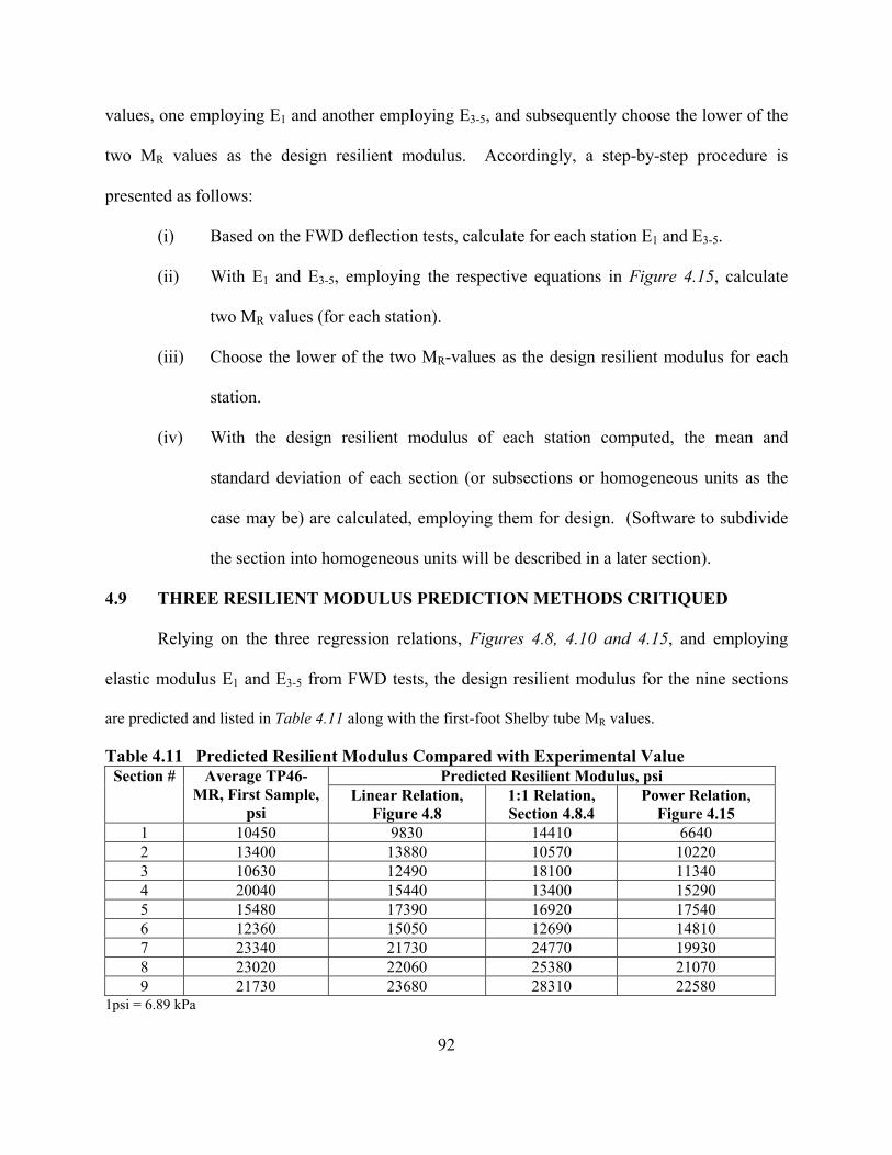
4.9 Three Resilient Modulus Prediction Methods Critiqued………………………...91 4.10 Data Analysis Software…………………………………………………………..93 4.11 Summary…………………………………………………………………………94
5. PLANNING FWD TEST AND CALCULATION OF DESIGN RESILIENT MODULUS……………………………………………………………………………...95 5.1 Overview…………………………………………………………………………95 5.2 Planning FWD Test in the Field…………………………………………………95
5.2.1 Equipment Selection……………………………………………………..96 5.2.2 When and Where To Test?………………………………………………97
5.3 Selection of Design Unit…………………………………………………………97 5.4 Computer Program, FWDSUBGRADE, to Calculation Design Modulus………99 5.5 Summary………………………………………………………………………..100
6. SUMMARY AND CONCLUSIONS…………………………………………………103
6.1 Summary………………………………………………………………………..103 6.2 Conclusions……………………………………………………………………..104 6.3 Recommendations for Further Research………………………………………..105 6.4 Implementation…………………………………………………………………106 6.5 Benefits…………………………………………………………………………106
REFERENCES…………………………………………………………………..……………108
APPENDIX A (FWD Deflection Basins, Typical Station From Each Section)………………113
APPENDIX B (Automated Dynamic Cone Penetrometer Test Data)…………………………119
APPENDIX C (Resilient Modulus of Sample 1 (0-12 in. Depth) As Function
of Stress State………………………………………………………………...…125
APPENDIX D (Detailed Flow Chart of Software Program FWDSUBGRADE)……………...148
viii
LIST OF TABLES 2.1 Summary of the Median and Mean Values for Each Coefficient of Constitutive
Equation 2.6 for Subgrade Soils, k6 = 0 (37)…………………………………………….14
2.2 AASHTO Modulus Correction Values From Long-term Pavement Performance Sections (43). (Backcalculated values shall be multiplied by a correction factor to get resilient modulus)…………………………………………………………………………………16
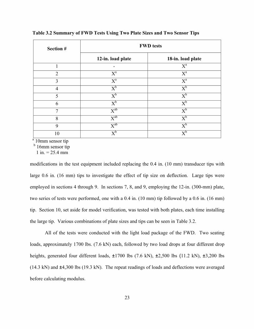
3.1 Summary Section Locations and Tests Performed………………………………………22 3.2 Summary of FWD Tests Using Two Plate Sizes and Two Sensor Tip Sizes……….…...23 3.3 Backcalculated Moduli Based on FWD Deflection Basin, Section # 1…………………...25 3.4 Comparison of Modulus (Expressed As A Ratio) Calculated for Offset Sensors Employing
Equation 3.1, and Exact Equation with Distributed Loads…………………………..……27 3.5 Elastic Moduli For All Four Load Drops For Nine Stations of Section # 4……………….28 3.6 Summary of Elastic Modulus Calculated from FWD Sensor Deflections Using
18-in. (450-mm) Plate, Montgomery County, Section # 1………………………………29 3.7 Summary of Elastic Modulus Calculated from FWD Sensor Deflections Using 18-in. (450-mm) Plate, Coahoma County, Section # 2…………………………………..29 3.8 Summary of Elastic Modulus Calculated from FWD Sensor Deflections Using 18-in.
(450-mm) Plate, Coahoma County, Section # 3…………………………………………30 3.9 Summary of Elastic Modulus Calculated from FWD Sensor Deflections Using 18-in.
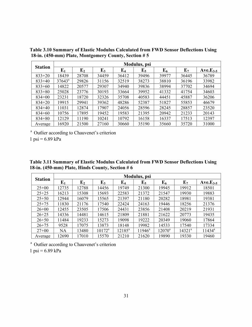
(450-mm) Plate, Montgomery County, Section # 4……………………………………..30 3.10 Summary of Elastic Modulus Calculated from FWD Sensor Deflections Using 18-in.
(450-mm) Plate, Montgomery County, Section # 5……………………………………..31 3.11 Summary of Elastic Modulus Calculated from FWD Sensor Deflections Using 18-in.
(450-mm) Plate, Hinds County, Section # 6…………………………………………….31 3.12 Summary of Elastic Modulus Calculated from FWD Sensor Deflections Using 18-in.
(450-mm) Plate, Wayne County, Section # 7……………………………………………32 3.13 Summary of Elastic Modulus Calculated from FWD Sensor Deflections Using 18-in.
(450-mm) Plate, Wayne County, Section # 8……………………………………………32 3.14 Summary of Elastic Modulus Calculated from FWD Sensor Deflections Using 18-in.
(450-mm) Plate, Wayne County, Section # 9……………………………………………33
ix
3.15 Summary of Elastic Modulus Calculated from FWD Sensor Deflections Using 18-in. (450-mm) Plate, Madison County, Section #10………………………………………….33
3.16 Summary of Elastic Modulus Calculated from FWD Sensor Deflections Using 12-in.
(300-mm) Plate, Coahoma County, Section #2………………………………………….34 3.17 Summary of Elastic Modulus Calculated from FWD Sensor Deflections Using 12-in.
(300-mm) Plate, Coahoma County, Section #3………………………………………….34 3.18 Summary of Elastic Modulus Calculated from FWD Sensor Deflections Using 12-in.
(300-mm) Plate, Montgomery County, Section #4………………………………………35 3.19 Summary of Elastic Modulus Calculated from FWD Sensor Deflections Using 12-in.
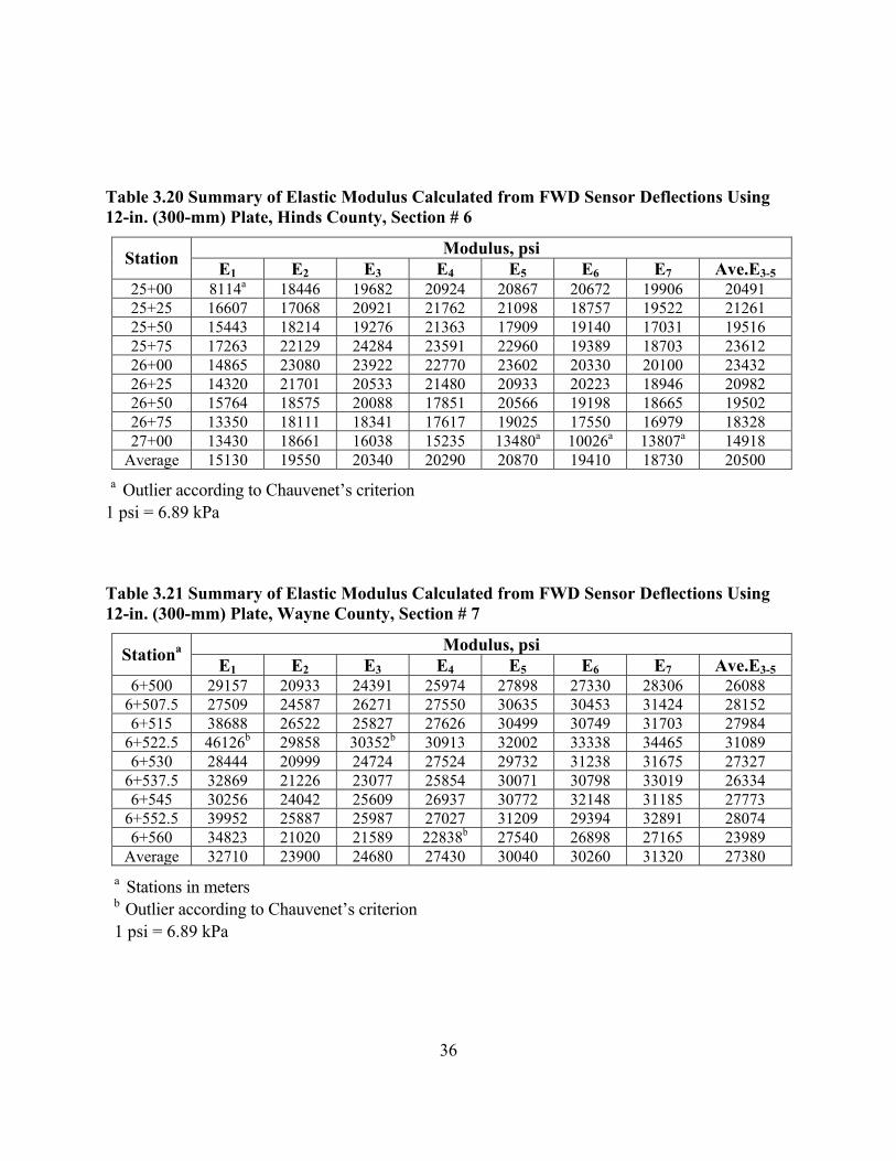
(300-mm) Plate, Montgomery County, Section #5………………………………………35 3.20 Summary of Elastic Modulus Calculated from FWD Sensor Deflections Using 12-in.
(300-mm) Plate, Hinds County, Section #6……………………………………………...36 3.21 Summary of Elastic Modulus Calculated from FWD Sensor Deflections Using 12-in.
(300-mm) Plate, Wayne County, Section #7…………………………………………….36 3.22 Summary of Elastic Modulus Calculated from FWD Sensor Deflections Using 12-in.
(300-mm) Plate, Wayne County, Section #8…………………………………………….37 3.23 Summary of Elastic Modulus Calculated from FWD Sensor Deflections Using 12-in.
(300-mm) Plate, Wayne County, Section #9…………………………………………….37 3.24 Summary of Elastic Modulus Calculated from FWD Sensor Deflections Using 12-in.
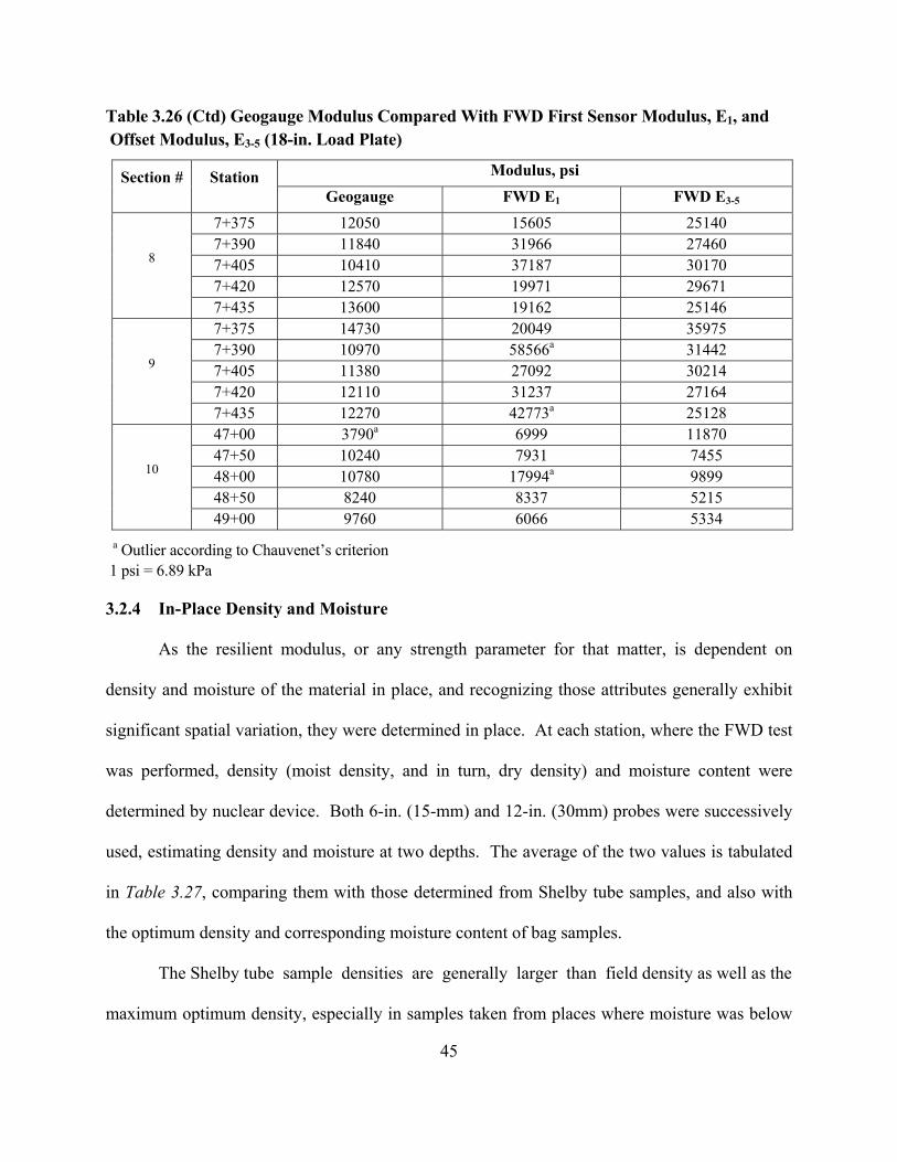
(300-mm) Plate, Madison County, Section #10………………………………………….38 3.25 Summary of Dynamic Cone Penetration Index (DCPI) Results of Ten Test Sections…..43 3.26 Geogauge Modulus Compared With FWD First Sensor Modulus, E1, and Offset Modulus,
3.27 Density and Moisture Determined (i) by Nuclear Device (ii) from Shelby Tube Samples, and (iii) Optimum Moisture and Density………………………………………………….46
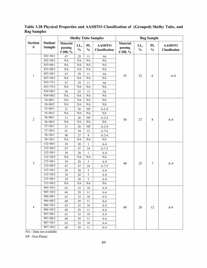
3.28 Physical Properties and AASHTO Classification of (Grouped) Shelby Tube, and Bag
Samples…………………………………………………………………………………...49 3.29 Resilient Modulus of Reconstituted Samples Compared With Modulus of Shelby Tube
Samples…………………………………………………………………………………...52 4.1 TP46 Resilient Modulus Compared to That Predicted by Equation 4.2…………………62
x
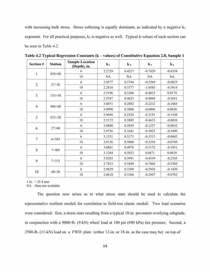
4.2 Typical Regression Constants (k – values) of Constitutive Equation 2.8, Sample 1…….64 4.3 Calculated Stress States in Subgrade Under Different Loads Including Overburden…...65 4.4 Resilient Modulus Calculated Employing Two Stress States at Depths 6 in. Below and 18
in. Below Surface, Respectively. Load 2500 lb on 18-in. Plate…………………………66 4.5 Comparison of Average Density and Moisture of Sample 1 (0 - 12 in. depth) and sample
2 (12 - 24 in. depth) Shelby Tube Samples………………………………………………67 4.6 Comparison of Coefficient of Variation of Sample 1 (0 - 12 in. depth) and Sample 2 (12 -
24 in. depth) Resilient Modulus………………………………………………………….68 4.7 Summary of Statistical Test Results Comparing 18-in. (450-mm) Plate Modulus to 12-in.
(300-mm) Plate Modulus………………………………………………………………...70 4.8 Comparison of Coefficient of Variation of 12-in. and 18-in. Plate Moduli……………..70 4.9 Average Section Elastic Moduli at Each Sensor, Load Plate = 12 in., Sensor Tip
10 mm/18 mm, Sections 7 – 9………………………………………………………..….72 4.10 How Sensor Tips, 10 mm and 16 mm, Affect Elastic Moduli (E1 and E3-5),
12-in. Plate……………………………………………………………………………….72 4.11 Predicted Resilient Modulus Compared with Experimental Value……………………...91
xi
LIST OF FIGURES 2.1 Typical FWD Load Impulse and Geophone Response With Time……………………...11 2.2 Frequency Response Function…………………………………………………………...12 3.1.a Elastic Moduli at Each Sensor Location. Nine Stations of Section #4, 1 psi = 6.89 kPa, 1 in. = 25.4 mm…………………………………………………………………………..38 3.1.b Elastic Moduli at Each Sensor Location. Nine Stations of Section #7, 1 psi = 6.89 kPa,
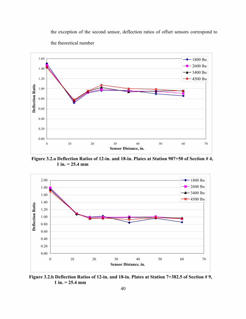
1 in. = 25.4 mm……………………………………………………………...…………...39 3.2.a Deflection Ratios of 12-in. and 18-in. Plates at Station 907+50 of Section #4, 1 in. = 25.4 mm……………………………………...…………………………………...40 3.2.b Deflection Ratios of 12-in. and 18-in. Plates at Station 7+382.5 of Section #9, 1 in. = 25.4 mm…………………...……………………………………………………...40 4.1 Geogauge Modulus Compared with FWD Modulus, E1(av), Section Averages,
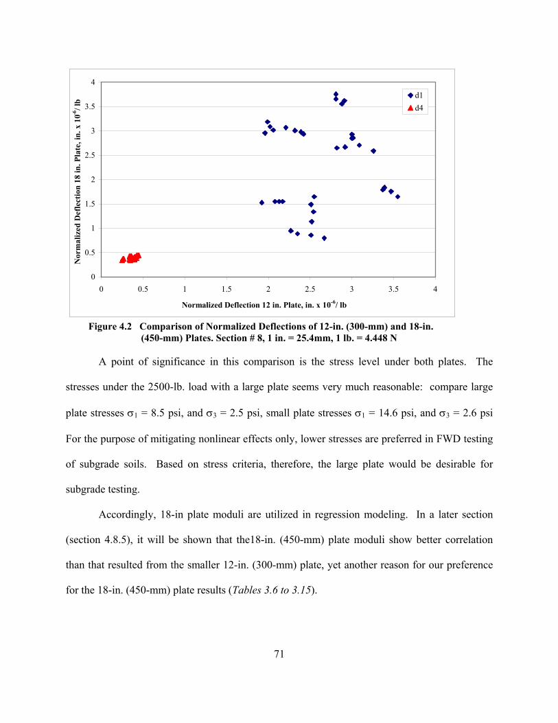
FWD with 18-in. (450-mm) Plate, 1 psi = 6.89 kPa…………………………………..…58 4.2 Comparison of Normalized Deflections of 12-in. (300-mm) and 18-in.(450-mm) Plates.
Section #8, 1 in. = 25.4mm, 1 lb. = 4.448N……………………………………………...71
4.3 Comparison of Normalized Deflections of 10 mm and 16 mm tip, Section # 8, 12-in. Plate, 1 in. = 25.4 mm……………………………………...…………………………….74
4.4 Photograph of Imprint Showing Loose Coarse Particles Congregating Around the First Sensor Tip………………………………………………………………………………..76
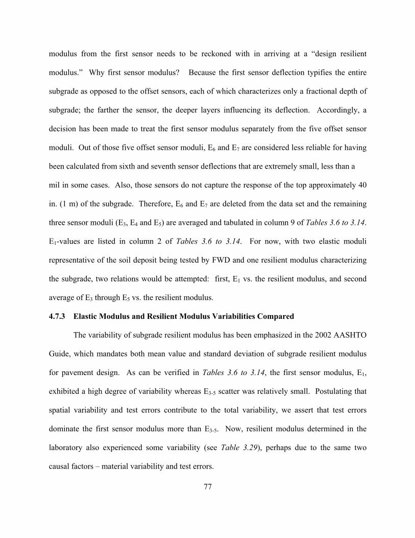
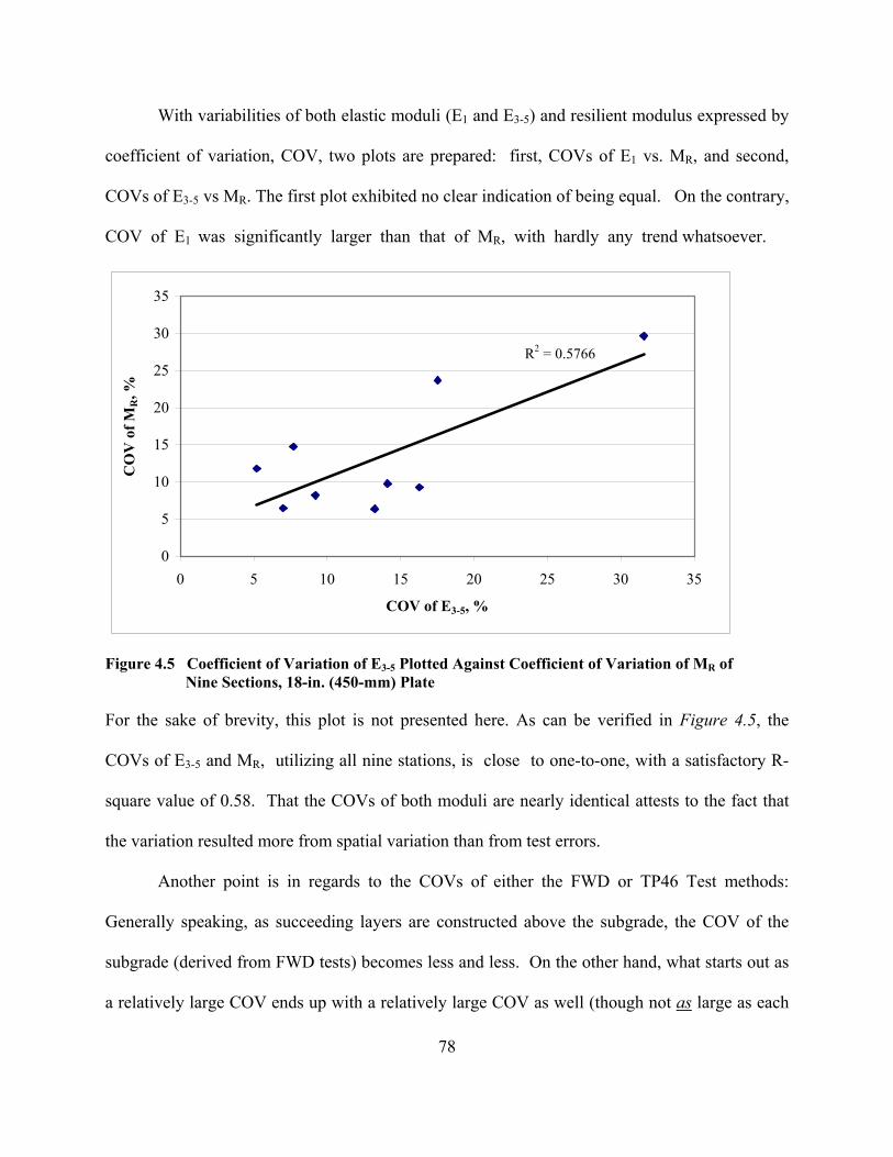
4.5 Coefficient of Variation of E3-5 Plotted Against Coefficient of Variation of MR of Nine Sections, 18-in. (450-mm) Plate…………………………………………………………78
4.6 Scatter Plot of Station-by-Station Values of E1 and MR, Nine Sections, 18-in. (450-mm) Plate, 1 psi = 6.89 kPa……………………………………………………………………81
4.7 Scatter Plot of Station-by-Station Values of E1 and MR, Eight Sections, (Section 1 Not Included), 12-in. (300-mm) Plate, 1 psi = 6.89 kPa……………………………………...81
4.8 Scatter Plot of Section Average E1 vs. Section Average MR, Nine Sections, 18-in. (450-mm) Plate, 1 psi = 6.89 kPa………………………………………………………..82
4.9 Scatter Plot of Section Average E3-5 vs. Section Average MR, Nine Sections, 18-in. (450-mm) Plate, 1 psi = 6.89 kPa………………………………………………………..84
4.10 Scatter Plot of Section Average E1 vs. Section Average MR, Nine Sections, 18-in.
4.11 Scatter Plot of Section Average E3-5 vs. Section Average MR, Nine Sections, 18-in. (450-mm) Plate, Intercept Zero, 1 psi = 6.89 kPa………………………………………..85
4.12 E1 and E3-5 Each Plotted Against Resilient Modulus MR, (Station-by-Station Values), Nine Sections, 18-in. (450-mm) Plate, 1 psi = 6.89 kPa…………………………………87
4.13 Scatter Plot of Station-by-Station Values of E1 and MR, 18-in. (450-mm) Plate, 1 psi = 6.89 kPa…………………………………………………………………………..88
4.14 Scatter Plot of Average Modulus of Sensors 3-5 vs. Resilient Modulus, 18-in. (450-mm) Plate, 1 psi = 6.89 kPa………………………………………………………..88
4.15 Section Averages E1 and E3-5, Each Plotted Against Average Resilient Modulus MR, Eight Sections, 18-in. (450-mm) Plate, Section 1 Deleted in E1 vs. MR Plot & Section 5 Deleted in E3-5 vs. MR Plot, 1 psi = 6.89 kPa…………………………………………….89
5.1 FN(40) Results versus Distance Along Project (Adapted From Reference 2)…………..98 5.2 Delineating Analysis Units by Cumulative Difference Approach (Adapted From
Reference 2)…………………………………………………………………………….100
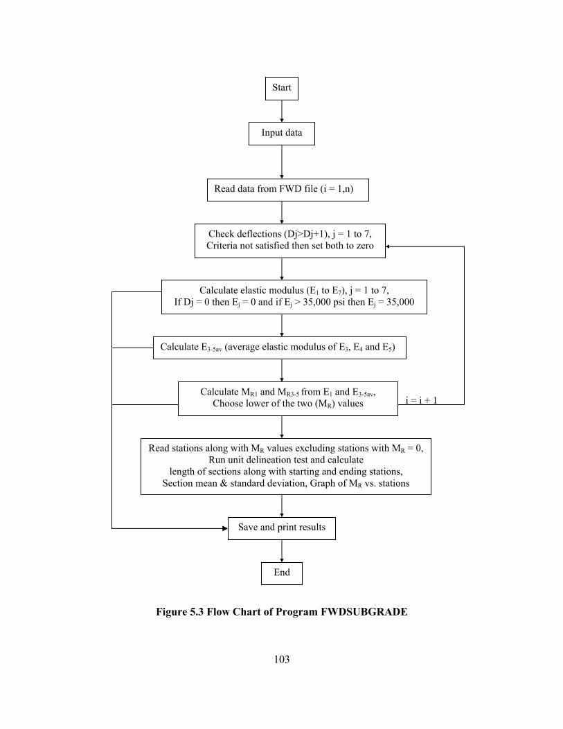
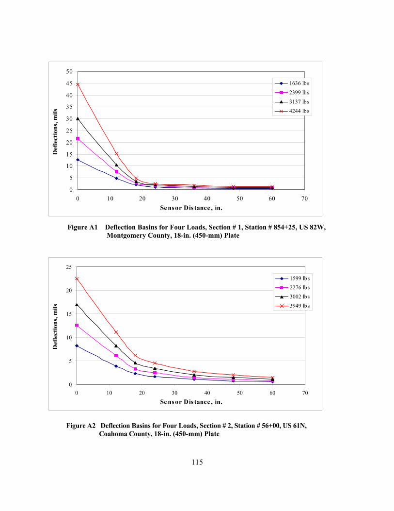
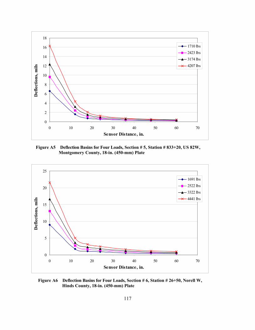
5.3 Flow Chart of Program FWDSUBGRADE…………………………………………….102 APPENDIX A FWD DEFLECTION BASINS, TYPICAL STATION FROM EACH SECTION……….113 Figure A1 Deflection Basins for Four Loads, Section #1, Station #854+25, US 82W, Montgomery County, 18-in. (450-mm) Plate…………………………………..114 Figure A2 Deflection Basins for Four Loads, Section #2, Station #56+00, US 61N, Coahoma County, 18-in. (450-mm) Plate………………………………………114 Figure A3 Deflection Basins for Four Loads, Section #3, Station #152+50, US 61N, Coahama County, 18-in. (450-mm) Plate………………………………………115 Figure A4 Deflection Basins for Four Loads, Section #4, Station #907+50, US 82W, Montgomery County, 18-in. (450-mm) Plate…………………………………..115 Figure A5 Deflection Basins for Four Loads, Section #5, Station #833+20, US 82W, Montgomery County, 18-in. (450-mm) Plate…………………………………..116 Figure A6 Deflection Basins for Four Loads, Section #6, Station #26+50, Norell W, Hinds County, 18-in. (450-mm) Plate…………………………………………..116
xiii
Figure A7 Deflection Basins for Four Loads, Section #7, Station #6+530, US 45N, Wayne County, 18-in. (450-mm) Plate…………………………………………117 Figure A8 Deflection Basins for Four Loads, Section #8, Station #7+405, US 45N, Wayne County, 18-in. (450-mm) Plate…………………………………………117 Figure A9 Deflection Basins for Four Loads, Section #9, Station #7+435, US 45N, Wayne County, 18-in. (450-mm) Plate…………………………………………118 Figure A10 Deflection Basins for Four Loads, Section #10, Station #48+50, Nissan W. Parkway, Madison County, 18-in. (450-mm) Plate…………………………….118 APPENDIX B AUTOMATED DYNAMIC CONE PENETROMETER TEST DATA…………………...119 Figure B1 ADCP Test Results in Section #1, US 82W, Montgomery County…………….120 Figure B2 ADCP Test Results in Section #2, US 61N, Coahoma County………………...120 Figure B3 ADCP Test Results in Section #3, US 61N, Coahoma County………………...121 Figure B4 ADCP Test Results in Section #4, US 82W, Montgomery County…………….121 Figure B5 ADCP Test Results in Section #5, US 82W, Montgomery County…………….122 Figure B6 ADCP Test Results in Section #6, Norrell W, Hinds County………………….122 Figure B7 ADCP Test Results in Section #7, US 45N, Wayne County…………………...123 Figure B8 ADCP Test Results in Section #8, US 45N, Wayne County…………………...123 Figure B9 ADCP Test Results in Section #9, US 45N, Wayne County…………………...124 Figure B10 ADCP Test Results in Section #10, Nissan W. Parkway, Madison County………124
APPENDIX C RESILIENT MODULUS OF SAMPLE # 1 (0 – 12 in. DEPTH) AS FUNCTION OF STRESS STATE………………………………………………………………………………125 Figure C1 Resilient Modulus Test Results, Station 852+50, Section 1, Sample #1,
1 MPa = 145 psi………………………………………………………………..126 Figure C2 Resilient Modulus Test Results, Station 853+50, Section 1, Sample #1,
1 MPa = 145 psi………………………………………………………………..126 Figure C3 Resilient Modulus Test Results, Station 853+75, Section 1, Sample #1,
1 MPa = 145 psi………………………………………………………………..127
xiv
Figure C4 Resilient Modulus Test Results, Station 854+00, Section 1, Sample #1, 1 MPa = 145 psi………………………………………………………………...127
Figure C5 Resilient Modulus Test Results, Station 55+00, Section 2, Sample #1,
1 MPa = 145 psi………………………………………………………………..128 Figure C6 Resilient Modulus Test Results, Station 56+00, Section 2, Sample #1,
1 MPa = 145 psi………………………………………………………………...128 Figure C7 Resilient Modulus Test Results, Station 57+50, Section 2, Sample #1,
1 MPa = 145 psi………………………………………………………………...129 Figure C8 Resilient Modulus Test Results, Station 58+50, Section 2, Sample #1,
1 MPa = 145 psi………………………………………………………………...129 Figure C9 Resilient Modulus Test Results, Station 152+00, Section 3, Sample #1,
1 MPa = 145 psi………………………………………………………………...130 Figure C10 Resilient Modulus Test Results, Station 152+50, Section 3, Sample #1,
1 MPa = 145 psi………………………………………………………………...130 Figure C11 Resilient Modulus Test Results, Station 153+00, Section 3, Sample #1,
1 MPa = 145 psi………………………………………………………………...131 Figure C12 Resilient Modulus Test Results, Station 153+50, Section 3, Sample #1,
1 MPa = 145 psi………………………………………………………………...131 Figure C13 Resilient Modulus Test Results, Station 153+90, Section 3, Sample #1,
1 MPa = 145 psi………………………………………………………………...132 Figure C14 Resilient Modulus Test Results, Station 905+50, Section 4, Sample #1,
1 MPa = 145 psi………………………………………………………………...132 Figure C15 Resilient Modulus Test Results, Station 906+00, Section 4, Sample #1,
1 MPa = 145 psi………………………………………………………………...133 Figure C16 Resilient Modulus Test Results, Station 906+50, Section 4, Sample #1,
1 MPa = 145 psi………………………………………………………………...133 Figure C17 Resilient Modulus Test Results, Station 907+00, Section 4, Sample #1,
1 MPa = 145 psi………………………………………………………………...134 Figure C18 Resilient Modulus Test Results, Station 907+50, Section 4, Sample #1,
1 MPa = 145 psi………………………………………………………………...134
xv
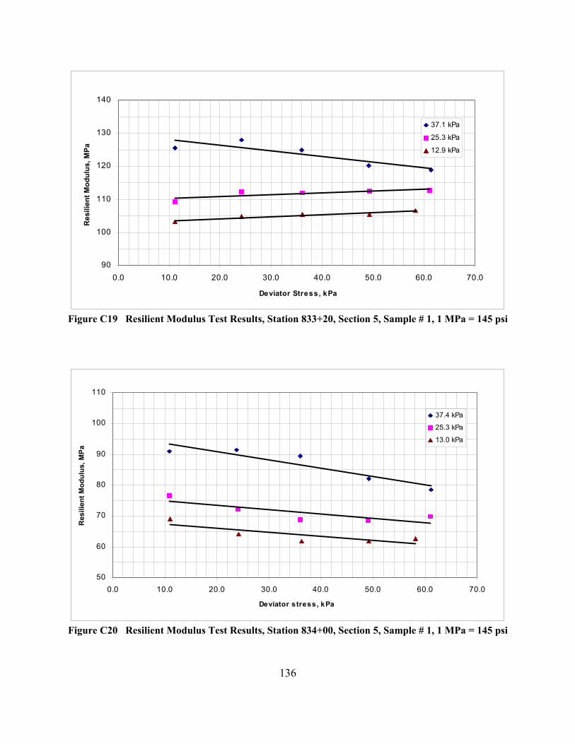
Figure C19 Resilient Modulus Test Results, Station 833+20, Section 5, Sample #1, 1 MPa = 145 psi………………………………………………………………...135
Figure C20 Resilient Modulus Test Results, Station 834+00, Section 5, Sample #1,
1 MPa = 145 psi………………………………………………………………...135 Figure C21 Resilient Modulus Test Results, Station 834+40, Section 5, Sample #1,
1 MPa = 145 psi………………………………………………………………...136 Figure C22 Resilient Modulus Test Results, Station 25+00, Section 6, Sample #1,
1 MPa = 145 psi………………………………………………………………..136 Figure C23 Resilient Modulus Test Results, Station 25+50, Section 6, Sample #1,
1 MPa = 145 psi………………………………………………………………..137 Figure C24 Resilient Modulus Test Results, Station 26+00, Section 6, Sample #1,
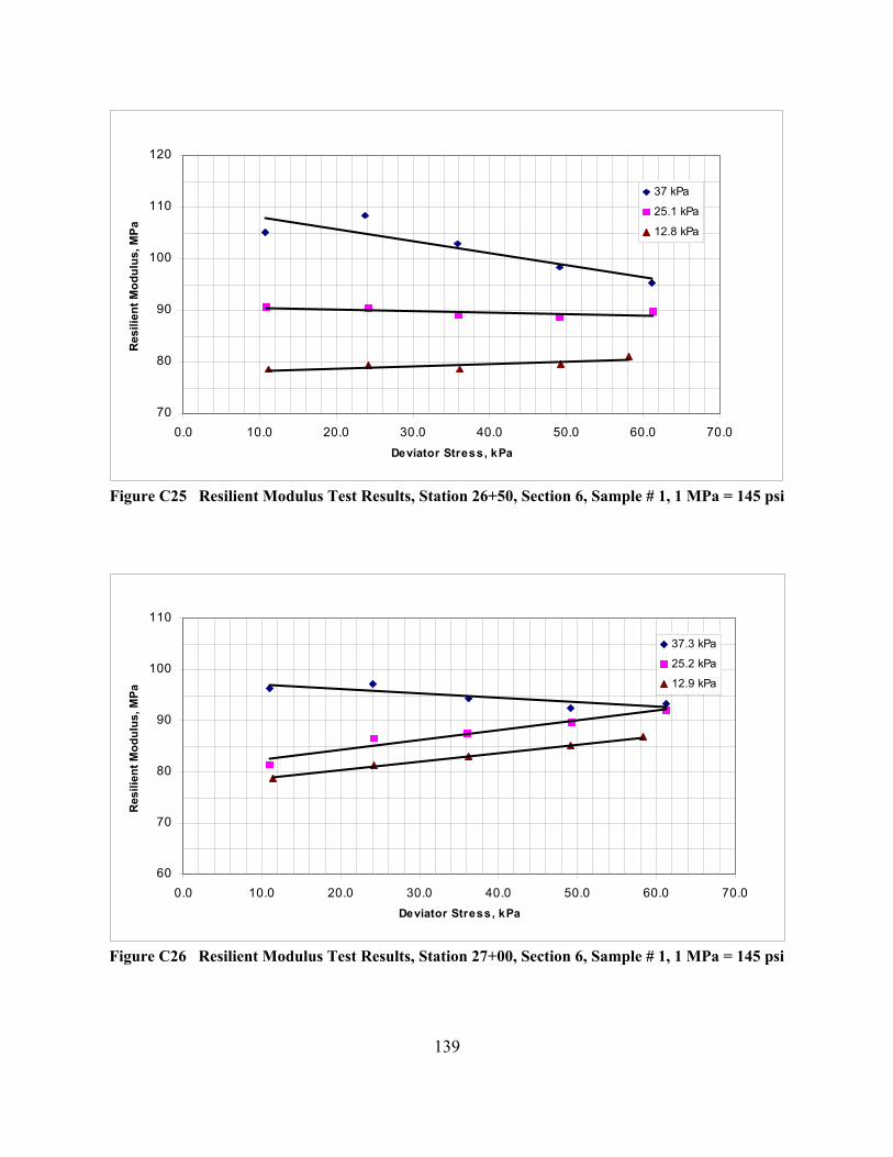
1 MPa = 145 psi………………………………………………………………..137 Figure C25 Resilient Modulus Test Results, Station 26+50, Section 6, Sample #1,
1 MPa = 145 psi……………………………………………………………….138 Figure C26 Resilient Modulus Test Results, Station 27+00, Section 6, Sample #1,
1 MPa = 145 psi……………………………………………………………….138 Figure C27 Resilient Modulus Test Results, Station 6+500, Section 7, Sample #1,
1 MPa = 145 psi……………………………………………………………….139 Figure C28 Resilient Modulus Test Results, Station 6+515, Section 7, Sample #1,
1 MPa = 145 psi……………………………………………………………….139 Figure C29 Resilient Modulus Test Results, Station 6+530, Section 7, Sample #1,
1 MPa = 145 psi……………………………………………………………….140 Figure C30 Resilient Modulus Test Results, Station 6+545, Section 7, Sample #1,
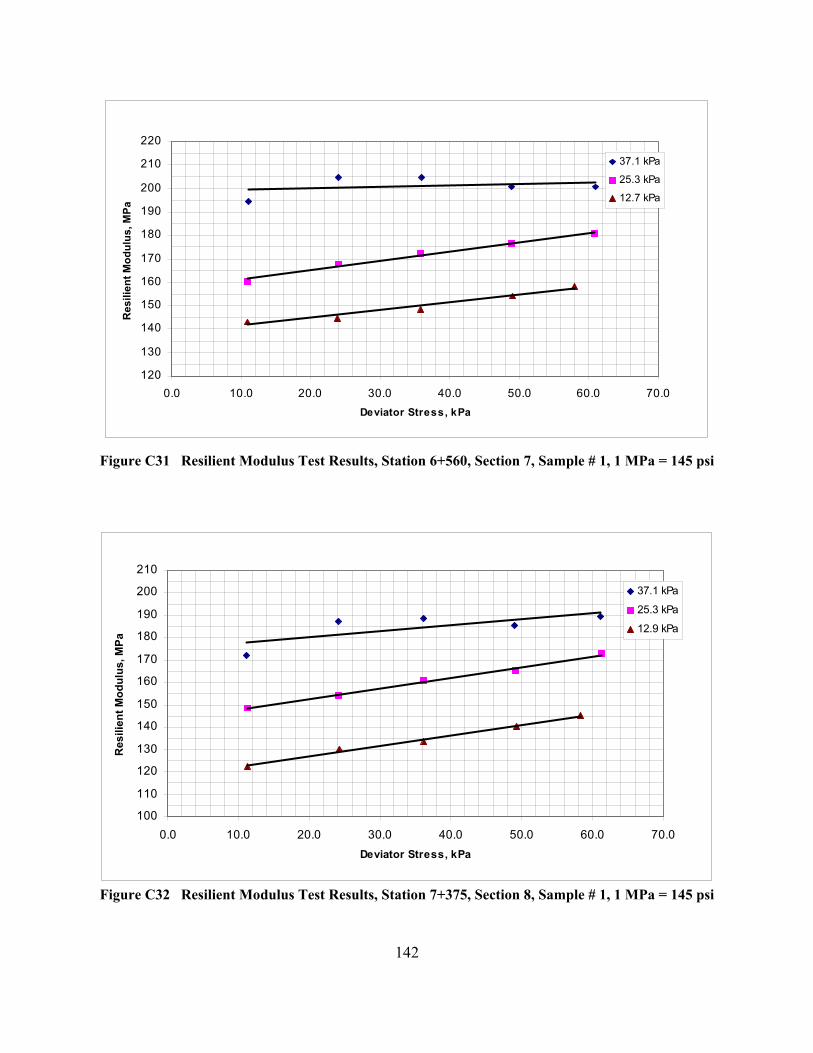
1 MPa = 145 psi……………………………………………………………….140 Figure C31 Resilient Modulus Test Results, Station 6+560, Section 7, Sample #1,
1 MPa = 145 psi………………………………………………………………141 Figure C32 Resilient Modulus Test Results, Station 7+375, Section 8, Sample #1,
1 MPa = 145 psi………………………………………………………………141 Figure C33 Resilient Modulus Test Results, Station 7+390, Section 8, Sample #1,
1 MPa = 145 psi………………………………………………………………142
xvi
Figure C34 Resilient Modulus Test Results, Station 7+405, Section 8, Sample #1, 1 MPa = 145 psi………………………………………………………………...142
Figure C35 Resilient Modulus Test Results, Station 7+420, Section 8, Sample #1,
1 MPa = 145 psi………………………………………………………………...143 Figure C36 Resilient Modulus Test Results, Station 7+375, Section 9, Sample #1,
1 MPa = 145 psi………………………………………………………………...143 Figure C37 Resilient Modulus Test Results, Station 7+390, Section 9, Sample #1,
1 MPa = 145 psi………………………………………………………………...144 Figure C38 Resilient Modulus Test Results, Station 7+420, Section 9, Sample #1,
1 MPa = 145 psi………………………………………………………………...144 Figure C39 Resilient Modulus Test Results, Station 7+435, Section 9, Sample #1,
1 MPa = 145 psi………………………………………………………………...145 Figure C40 Resilient Modulus Test Results, Station 47+00, Section 10, Sample #1,
1 MPa = 145 psi………………………………………………………………...145 Figure C41 Resilient Modulus Test Results, Station 47+50, Section 10, Sample #1,
1 MPa = 145 psi………………………………………………………………...146 Figure C42 Resilient Modulus Test Results, Station 48+00, Section 10, Sample #1,
1 MPa = 145 psi………………………………………………………………...146 Figure C43 Resilient Modulus Test Results, Station 48+50, Section 10, Sample #1,
1 MPa = 145 psi………………………………………………………………...147 Figure C44 Resilient Modulus Test Results, Station 49+00, Section 10, Sample #1,
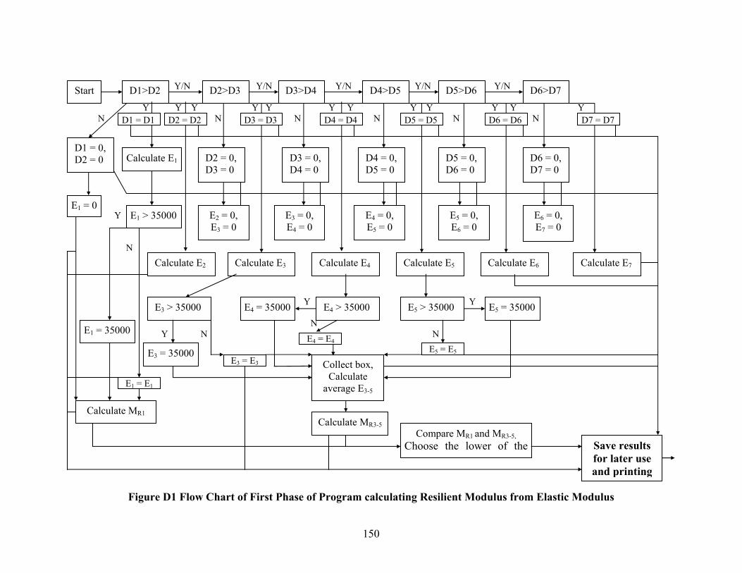
1 MPa = 145 psi………………………………………………………………...147 APPENDIX D DETAILED FLOWCHARTS OF SOFTWARE PROGRAM FWDSUBGRADE……….148 Figure D1 Flow Chart of First Phase of Program calculating Resilient Modulus from
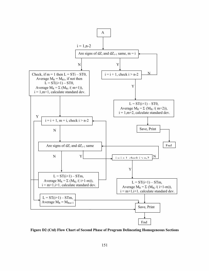
Elastic Modulus………………………………………………………………...149 Figure D2 Flow Chart of Second Phase of Program Delineating Homogeneous Section…150
1
CHAPTER 1
INTRODUCTION
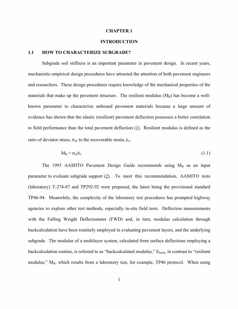
1.1 HOW TO CHARACTERIZE SUBGRADE?
Subgrade soil stiffness is an important parameter in pavement design. In recent years,
mechanistic-empirical design procedures have attracted the attention of both pavement engineers
and researchers. These design procedures require knowledge of the mechanical properties of the
materials that make up the pavement structure. The resilient modulus (MR) has become a well-
known parameter to characterize unbound pavement materials because a large amount of
evidence has shown that the elastic (resilient) pavement deflection possesses a better correlation
to field performance than the total pavement deflection (1). Resilient modulus is defined as the
ratio of deviator stress, σd, to the recoverable strain, εr,
MR = σd/εr (1.1)
The 1993 AASHTO Pavement Design Guide recommends using MR as an input
parameter to evaluate subgrade support (2). To meet this recommendation, AASHTO tests
(laboratory) T-274-87 and TP292-92 were proposed, the latest being the provisional standard
TP46-94. Meanwhile, the complexity of the laboratory test procedures has prompted highway
agencies to explore other test methods, especially in-situ field tests. Deflection measurements
with the Falling Weight Deflectometer (FWD) and, in turn, modulus calculation through
backcalculation have been routinely employed in evaluating pavement layers, and the underlying
subgrade. The modulus of a multilayer system, calculated from surface deflections employing a
backcalculation routine, is referred to as “backcalculated modulus,” Eback, in contrast to “resilient
modulus,” MR, which results from a laboratory test, for example, TP46 protocol. When using
2
forward calculation, employing surface deflection(s) and Boussinesq equations, the modulus
resulting is designated “elastic modulus,” E.
Highway agencies have also attempted to correlate resilient modulus with other test
parameters. The California Bearing Ratio (CBR)-resilient modulus correlation has been studied
extensively (3). The Dynamic Cone Penetrometer (DCP), a penetration device, introduced in the
1960s for pavement evaluation, is another device that has been employed for characterization for
subgrade soils (4, 5, 6, 7).
The AASHTO Guide allows the use of both laboratory and in situ backcalculated moduli,
but recognizes that the moduli determined by both procedures are not equal. The guide,
therefore, suggests that the subgrade modulus determined from deflection measurements on the
pavement surface, Eback, be adjusted by a factor of 0.33. However, other ratios have been
documented. Ali and Khosla (8) compared the subgrade soil resilient modulus determined in the
laboratory and backcalculated values from three pavement sections in North Carolina. The ratio
of laboratory- measured modulus values to the corresponding backcalculated values varied from
0.18 to 2.44. Newcomb (9) reported the results of similar tests in Washington State, suggesting a
ratio in the range of 0.8 to 1.3. Von Quintus et al. (10) reported ratios in the range of 0.1 to 3.5
in a study based on data obtained from the Long Term Pavement Performance (LTPP) database.
In the same reference, different average ratios were reported based on the type of layers atop the
subgrade layer. Laboratory values were consistently higher (nearly double) than the
backcalculated values, according to Chen et al. (11). Note that the previous studies relied on
backcalculated moduli from deflection measurements on the top of the pavement structure.
Many factors may have contributed to the disagreement between the laboratory measured and
backcalculated moduli. One reason is the difficulty of obtaining representative samples from the
3
field because of the inherent variability of the subgrade layer itself. A detailed discussion of the
differences between laboratory measured MR(lab) and backcalculated moduli can be found
elsewhere (12).
While numerous studies have attempted FWD measurements on the pavement surface,
only a few have targeted FWD tests conducted directly on the subgrade surfaces. In their study
of the Minnesota Research Road Project (Mn/ROAD), Van Deusen et al. (13) reported
difficulties analyzing FWD measurements performed directly on subgrade surfaces. Their
results showed a weak correlation between laboratory and backcalculated moduli. Chai (6)
employed the FWD during subgrade construction, backcalculated modulus and comparing these
values to the field modulus calculated from the Dynamic Cone Penetration Index (DCPI).
Resilient modulus vs. elastic modulus, E, relation was explored in a recent study titled “The
Virginia Smart Road Project” (14). The relationship, however, was less than satisfactory. A
recent investigation, conducted by the author’s group, showed that the backcalculated moduli
(Eback) obtained from testing directly on the subgrade are in satisfactory agreement with the
laboratory values with certain restrictions (15).
1.2 CRITIQUE OF RESILIENT MODULUS TEST (TP46)
Since AASHTO recommends using a laboratory resilient modulus test in a relatively small
soil sample – one that is undisturbed or reconstituted – it is worthwhile to examine how realistic
this test is. Despite several improvements made over the years, researchers have cited several
uncertainties as well as limitations associated with this laboratory test procedure, a list of which
follows (16):
1. The laboratory resilient modulus sample is not completely representative of in situ
conditions because of sample disturbance and differences in aggregate orientation,
4
moisture content, in-situ soil suction and level of compaction (or recompaction).
2. Inherent equipment flaws make it difficult to simulate the state of stress of the material in
situ.
3. Inherent instrumentation flaws create uncertainty in the measurement of sample
displacements.
4. Lack of uniform equipment calibration and verification procedures lead to differences not
only between labs but also within a given lab.
5. Laboratory specimens represent the properties of a small quantity of material, and not
necessarily the average of the mass of material that responds to a typical truck axle.
6. The time, expense and potential impact associated with a statistically adequate sampling
plan as well as testing add up to large expenditure.
Overall, these issues have kept the resilient modulus test from achieving general acceptance by
the pavement and materials testing community, whereas a nondestructive test such as the FWD
deflection test is credited with providing in situ modulus, and is also capable of identifying
inherent spatial variation. This research explores the viability of FWD in estimating subgrade
material modulus, a surrogate for resilient modulus for pavement design.
1.3 OBJECTIVE
This project addresses the issue of employing FWD deflection test data for subgrade
characterization. Recognizing the need for the resilient modulus of subgrade soil in AASHTO
design methodology, this research seeks a relationship between deflection-based elastic modulus,
E, and laboratory determined resilient modulus, MR. Once a statistically significant relationship
is established, the FWD could become a viable device for direct in-situ testing of subgrades and
for estimating the subgrade resilient modulus (via a derived relationship), the standard input into
5
the AASHTO 1993 Design Guide, as well as in the 2002 Mechanistic Design Guide.
1.4 SCOPE
Ten as-built subgrades, representing a wide range of soil types, were tested with
Mississippi Department of Transportation (MDOT) FWD employing the low-load package and
two load plates (12-in. (300-mm) and 18-in. (450-mm)). Shelby tube samples (three depths from
each station) were retrieved from the same locations and tested for resilient modulus, MR. For
direct verification of the stiffness of the subgrade, Geogauge modulus was determined at each
location. Side-by-side (automated) dynamic cone penetrometer tests were also performed, to a
depth of 3 ft. 3 in. (1000 mm), identifying layering of subgrade, which became useful in
interpreting deflection-based elastic modulus. Because of their importance on soil properties,
density and moisture were determined using nuclear gauge, again at the same test locations. Bag
samples collected from each section enabled us to identify and classify the soil in each test
section, further substantiating the classification test results of Shelby tube samples.
This report comprises six chapters and three appendices. Chapter 2 presents a literature
review of the use of deflection testing devices for material characterization with special reference
to FWD deflections for subgrade modulus calculation, and its relation to resilient modulus. Field
data collected from ten test sections, five stations from each test section, are presented in Chapter
3. A comprehensive data analysis, culminating in a relation between elastic modulus, E, and
resilient modulus, MR, comprises Chapter 4. A methodology for FWD tests is described in the
first part of chapter 5. Presented in the latter part is an outline of a computer program designated
“FWDSUBGRADE,” for analyzing FWD data, arriving at a design resilient modulus – mean and
standard deviation of so-called “uniform section.” A summary and observations regarding the
findings of the study constitute Chapter 6. Typical deflection basins are presented in Appendix
6
A. Appendix B includes the entire DCP data of ten test sections. Resilient modulus test results
comprise Appendix C. Detailed flow charts of the program, FWDSUBGRADE, are included in
Appendix D.
7
CHAPTER 2
REVIEW OF LITERATURE
2.1 INTRODUCTION
The 1986 AASHTO Guide has stipulated and the 2002 Guide reaffirmed that resilient
modulus should be the parameter for characterizing subgrade. Consequently, AASHTO Tests
(laboratory) T274-87 and TP292-91 were proposed, the latest being the provisional standard
TP46-94 and the “harmonized” MR test protocol developed in the NCHRP 1-28A study. The
complexity of the laboratory test procedures has prompted highway agencies to explore other test
methods, primarily nondestructive deflection tests, and subsequent backcalculation of moduli
(17). Some of the impulse devices currently in use are Falling Weight Deflectometer, Loadman,
and TRL Foundation Tester (TFT). Correlation of laboratory moduli with other test methods has
been attempted. The California Bearing Ratio–resilient modulus correlation has been studied
extensively in the past. The Dynamic Cone Penetrometer (DCP), a penetration device,
introduced in the 1960s for pavement evaluation, is another device that has been employed for
characterization of subgrade soils, again via a correlation between laboratory MR and DCP index
(4, 7).
2.2 DEFLECTION TESTS FOR MATERIAL CHARACTERIZATION
Nondestructive testing (NDT) of pavements, especially deflection testing, has been a vital
part evaluating the structural capacity of pavement. The following discusses different deflection
measuring methods and analysis techniques to derive material property of the layered system. A
detailed discussion of these topics can be seen in reference (18).
The NDT equipment used in making the measurements includes a variety of modes for
applying loads to a pavement and a number of sensors for measuring the pavement response.
8
The loading methods include: (a) static or slowly moving loads, (b) vibration, (c) “near field”
impulse methods, and (d) wave propagation methods. Output responses are measured on the
surface or with depth below the surface. Surface measurements are made with the following: (a)
geophones that sense the velocity of motion, (b) accelerometers, and (c) linear voltage
differential transformers (LVDT) that measure displacement. Measurements below the surface
are made with all of the same sensors, but the loading methods may include moving traffic.
The Benkelman Beam, the LaCroix Deflectograph, and the Curviameter apply static or
slow moving loads. Vibratory loads are applied by the Dynaflect, the Road Rater, the Corps of
Engineers 71-kN (16-kip) Vibrator, and the Federal Highway Administration’s Cox Van. “Near
field” impulse loads, a term which will be explained subsequently, are applied by the Dynatest,
KUAB, and Phoenix falling weight deflectometers. Small-scale impulse test devices include
Loadman (19), German Dynamic Plate Bearing Test (GBP) (20), and TRL Foundation Tester
(TFT) (21). “Far field” impulse loads are applied by the impact devices used in Spectral
Analysis of surface wave technique. Wave propagation is used by the Shell Vibrator, which
loads the pavement harmonically and sets up standing surface waves, the peaks and nodes of
which are found by using moveable sensors.
2.2.1 Deflection Analysis Methods
The analytical methods covered in this review are categorized as follows: (a) closed-
form multilayered solution, (b) backcalculation of moduli, and (c) impulse methods for near-field
measurements.
2.2.1.1 Closed-Form Multilayered Solution
The first closed-form, multilayer solution for the backcalculation of layer moduli was
developed by Hou (22). The central feature of this method was the least squares method
9
(Newton method) used for searching for the set of moduli that will reduce the sum of the squared
differences between the calculated and measured deflections to a minimum. An algorithm based
on the modified Newton method was employed by Harichandran et al. (23) to obtain the least
squares solution of an over-determined set of equations. The algorithm was implemented in a
new backcalculation program named MICHBACK.
Another closed-form solution makes use of Odemark’s assumption (24), which was
developed for the purpose of estimating surface deflections of multilayered pavements.
According to Odemark, the deflection of a multilayered pavement with moduli, Ei and layer
thickness, hi, may be represented by a single layer thickness, H, and a single modulus, E0, if the
thickness is chosen to be:
3/1
1 0∑=
∗∗=
m
i
i
EE
hCH i (2.1)
where, C = a constant, approximately 0.8 to 0.9
This useful assumption makes it possible to use the Boussinesq theory for a one-layer to
estimate stresses, strains, and displacements in the half-space, which are assumed to occur in the
real multilayered pavement at the same radius and at the depth corresponding to the transformed
depth where they were calculated.
An equivalent layer method of special mention here is the one developed by Ullidtz (25),
which permits the use of a stress-softening nonlinear stress-strain relation in the subgrade.
Calculations of rutting and fatigue life of test pavements, using strains and deflections computed
using this method, have proven to be realistic. Backcalculation of layer moduli also appears to
give reasonable results for pavements in which the layer decreases in stiffness with depth.
10
2.2.1.2 Backcalculation of Moduli
Backcalculation procedure is widely employed for analyzing deflection data from FWD.
There are three general techniques into which these methods may be grouped.
1. There is a traditional backcalculation technique that matches measured deflections
against those calculated from theory. Some of the programs that make use of this
technique include EVERCALC (26), MODCOMP (27), and WESDEF (28).
2. A pattern search technique is employed in MODULUS (29) to obtain a match between
measured and calculated deflections.
3. BOUSDEF (30) and ELMOD (31) are examples of a technique based on an equivalent
layer method.
The traditional backcalculation technique uses deflection test conditions (i.e., load,
plate geometry, layer thicknesses) and estimated layer moduli to generate a theoretical deflection
basin. The theoretical deflections are compared with the measured deflections, and the error is
computed. If the error is not within a specified tolerance, the process is repeated with revised
layer modulus values until the two deflection basins are considered to be sufficiently close or
until the modulus for any given layer reaches a given limit.
2.2.1.3 Impulse and Response Analysis Methods in the Near Field
When the falling weight drops to a pavement surface, an impulse generates body waves
and surface waves. The geophone sensors pick up the vertical velocity of the pavement surface,
and a single analog integration of the signal produces the deflection versus time trace. Figure 2.1
shows a typical set of force versus time impulses and deflection versus time responses. Usually
these signals are used to extract the maximum force and the maximum deflection from each
geophone and to print them out for analysis by elastic methods. But, there is much more useful
11
Figure 2.1 Typical FWD Load Impulse and Geophone Response With Time
information in these signals than simply their maxima.
One method of tapping this additional information is to perform a Fast Fourier Transform
on the force-time impulse and on each deflection-time response. The transform breaks up a
signal into its component frequencies and produces a complex number for each frequency, a(f) +
ib(f). The magnitude of this complex number is (a2 + b2)1/2, and the phase angle, Φ,
(arc tan (b/a)). If the transform of the deflection signal is divided, frequency-by-frequency, by
the transform of the load impulse, the result is a transfer function, which is also a complex
number and a function of frequency. A graph of the magnitude for typical transfer functions is
shown in Figure 2.2 for the geophones placed 1, 3, and 5 ft (0.3, 0.9, and 1.5m) from the center
of the loaded area. In Figure 2.2, the magnitude is the deflection per unit of force at each
frequency.
12
Figure 2.2 Frequency Response Function
2.3 NONLINEAR CHARACTERIZATION OF SUBGRADE (UNBOUND
MATERIAL)
Ever since resilient modulus officially replaced earlier design parameters such as soil
support value, its nonlinear behavior has been recognized. Ullditz (25) asserted that the
difference between field modulus and laboratory modulus can be overcome by treating the
subgrade as a nonlinear material. Over the years, numerous models have been proposed, a brief
review of which follows:
2
1
k
a
dR p
kM
=
σ (Moossadeh and Witczak (32)) (2.2)
2
31
k
aR p
kM
=
σ (Dunlap, (33)) (2.3)
13
2
1
k
aR p
kM
=
θ (Seed et al. (34)) (2.4)
where σd = deviator stress;
σ3 = confining pressure;
θ = bulk stress;
pa = atmospheric pressure; and
k1, k2 = regression constants.
May and Witczak (35) and Uzan (36) proposed another model
32
1
k
a
d
k
aR pp
kM
=
σθ (2.5)
An expanded version of Equation 2.5, that has been used is,
Coefficient k1 is proportional to Young’s modulus. Thus, the values for k1 should be positive
since MR can never be negative. Increasing the volumetric stress (θ) should produce a stiffening
or hardening of the material, which results in a higher MR. Therefore, the exponent k2 of the bulk
stress term for the above constitutive equation should also be positive. Coefficient k6 is intended
to account for pore water pressure or cohesion and is a measure of the material’s ability to resist
tension. The values for k6 are expected to be negative or, when positive, less than or equal to a
third of the bulk stress. Coefficient k3 is the exponent of the octahedral shear stress term, and
14
its value should be negative since increasing the shear stress will produce a softening of the
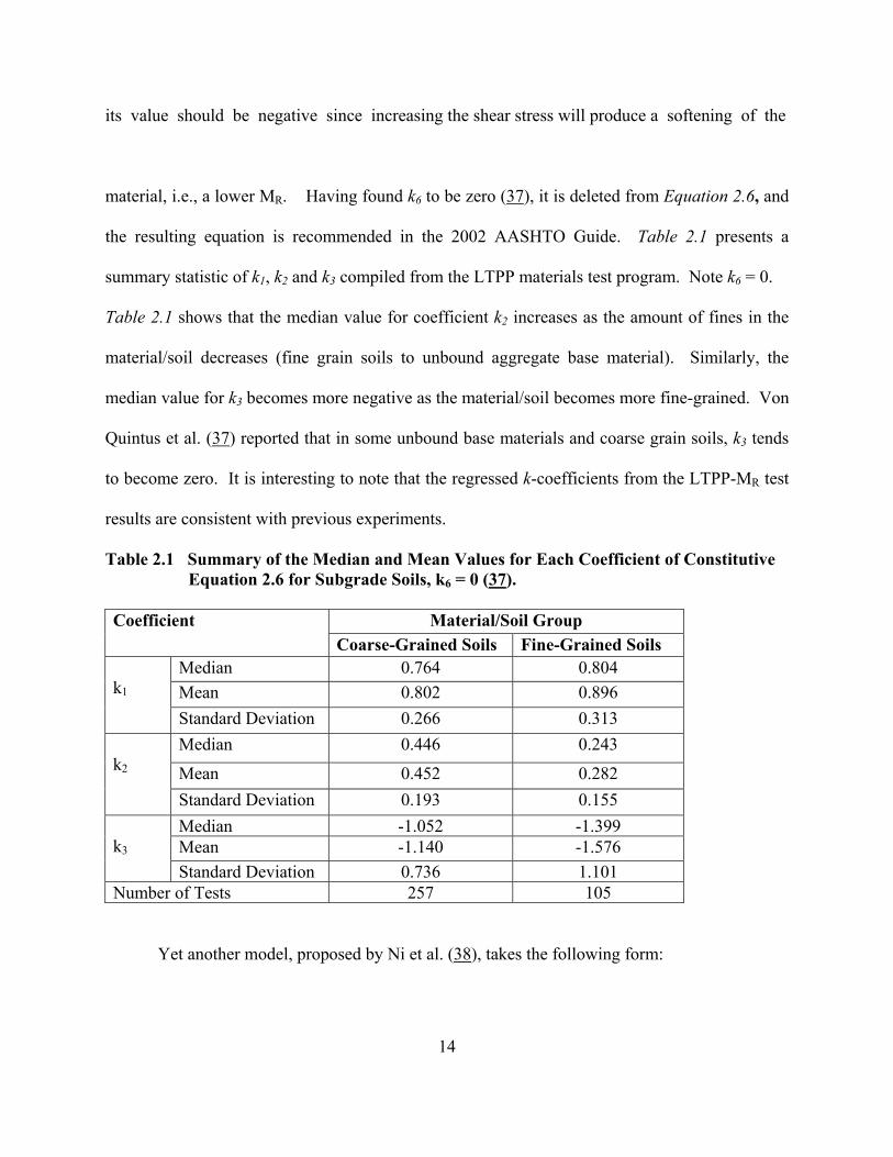
material, i.e., a lower MR. Having found k6 to be zero (37), it is deleted from Equation 2.6, and
the resulting equation is recommended in the 2002 AASHTO Guide. Table 2.1 presents a
summary statistic of k1, k2 and k3 compiled from the LTPP materials test program. Note k6 = 0.
Table 2.1 shows that the median value for coefficient k2 increases as the amount of fines in the
material/soil decreases (fine grain soils to unbound aggregate base material). Similarly, the
median value for k3 becomes more negative as the material/soil becomes more fine-grained. Von
Quintus et al. (37) reported that in some unbound base materials and coarse grain soils, k3 tends
to become zero. It is interesting to note that the regressed k-coefficients from the LTPP-MR test
results are consistent with previous experiments.
Table 2.1 Summary of the Median and Mean Values for Each Coefficient of Constitutive Equation 2.6 for Subgrade Soils, k6 = 0 (37).
Material/Soil Group Coefficient
Coarse-Grained Soils Fine-Grained Soils Median 0.764 0.804 Mean 0.802 0.896
k1
Standard Deviation 0.266 0.313 Median 0.446 0.243
Mean 0.452 0.282
k2
Standard Deviation 0.193 0.155 Median -1.052 -1.399 Mean -1.140 -1.576
k3
Standard Deviation 0.736 1.101 Number of Tests 257 105
Yet another model, proposed by Ni et al. (38), takes the following form:
15
32
1131
k
a
d
k
aR pp
kM
+
+=
σσ (2.7)
A recent LTPP study (39) included an additional power term to the universal model of Uzan,
2
4321 loglogloglog
+
+
+=
a
oct
a
oct
aa
R
pk
pk
pkk
pM ττθ (2.8)
According to the authors, there is a reasonably strong trend for the TP46 results to be somewhat
nonlinear for the log octahedral shear stress term. Nonlinear behavior of log bulk stress,
however, is not as common, but does exist in some cases.
2.4 RELATION BETWEEN RESILIENT MODULI, MR, AND FWD MODULUS, Eback
OR E
The results of comparison overwhelmingly suggest that the laboratory resilient modulus
is less than that determined from backcalculation, Eback. The AASHTO Guide (2) asserted that
laboratory modulus is only a third of that determined from in situ deflection of pavements. Other
researchers, for example, Daleiden (40), Akram (41) and Nazarian (42) could not identify a
unique relationship between moduli from laboratory and field tests. Having failed to establish a
meaningful relationship between laboratory and backcalculated moduli, Von Quintus and
Killingsworth (43) recommended correction factors (see Table 2.2) to be used with the AASHTO
Design Guide. Based on the comparison study performed in regard to the WESTRACK road
test, Seed et al. (16) asserted that their findings were enough to support the consensus that
laboratory and NDT-based backcalculated moduli do not agree.
Whereas all of the above investigations relied on FWD measurements on pavement
surface, only a few investigations had conducted the FWD test directly on the subgrade surface.
In their study of the Minnesota Research Road Project (Mn/ROAD), difficulties were
16
encountered in analyzing FWD measurements performed directly on a subgrade surface
(17). Their results showed weak correlation between laboratory and backcalculated moduli. Yet
another attempt to estimate resilient modulus via subgrade deflection testing and Boussinesq
Table 2.2 AASHTO Modulus Correction Values From Long-term Pavement Performance Sections (43). (Backcalculated value shall be multiplied by correction factor to get resilient modulus)
Layer Type and Location
C-Value, Correction Factor
Granular base/subbase under PCC 1.32 Granular base/subbase under AC 0.62 Granular base/subbase between stabilized layer and AC 1.43 Subgrade soils under stabilized subgrade 1.32 Subgrade under full-depth AC or PCC 0.52 Subgrade under granular base/subbase 0.35
Average 3240 3560 10590 14010 18630 16900 16480 14410 a Outlier according to Chauvenet’s criterion NA - Data not available 1 psi = 6.89 kPa Table 3.7 Summary of Elastic Modulus Calculated from FWD Sensor Deflections Using 18-in. (450-mm) Plate, Coahoma County, Section # 2
Average 8060 11420 18160 17700 18450 17090 16230 18100
a Outlier according to Chauvenet’s criterion 1 psi = 6.89 kPa Table 3.9 Summary of Elastic Modulus Calculated from FWD Sensor Deflections Using 18-in. (450-mm) Plate, Montgomery County, Section # 4
a Outlier according to Chauvenet’s criterion 1 psi = 6.89 kPa Table 3.11 Summary of Elastic Modulus Calculated from FWD Sensor Deflections Using 18-in. (450-mm) Plate, Hinds County, Section # 6
Average 28310 28000 28680 29240 31470 30290 29200 29800
a Stations in meters
b Outlier according to Chauvenet’s criterion 1 psi = 6.89 kPa Table 3.15 Summary of Elastic Modulus Calculated from FWD Sensor Deflections Using 18-in. (450-mm) Plate, Madison County, Section # 10
a Outlier according to Chauvenet’s criterion 1 psi = 6.89 kPa Table 3.19 Summary of Elastic Modulus Calculated from FWD Sensor Deflections Using 12-in. (300-mm) Plate, Montgomery County, Section # 5
Average 31290 25010 27360 27760 30880 28800 28010 28670
a Stations in meters b Outlier according to Chauvenet’s criterion 1 psi = 6.89 kPa Table 3.23 Summary of Elastic Modulus Calculated from FWD Sensor Deflections Using 12-in. (300-mm) Plate, Wayne County, Section # 9
the optimum. This could be attributed to disturbance/densification resulting from pushing
Shelby tube for sample extraction. Since MR is significantly affected by sample density,
modulus values could be higher for those samples. A correction to account for this re-
compaction effect was attempted, a description of which will be presented in a later section.
3.2.5 Soil Sampling and Tests
Two independent sampling procedures were performed: Shelby tube samples from every
station where FWD test was performed, and a bag sample representative of each test section.
Three Shelby tube samples were retrieved from each station, at 1 ft. (304 mm) intervals reaching
a depth in excess of 3 ft. (912 mm). These core samples were sealed in wax paper and shipped to
the laboratory for resilient modulus testing in accordance with TP 46 protocol. The coring not
only corroborated the layering, if any, identified by ADCP, but also helped to explore the
presence of possible water table/rigid bottom. In order for the bag sample to be representative of
the section, it was collected from three sampling locations digging to a depth of 16 in. (406 mm)
minimum. This composite sample was shipped to the laboratory for further tests.
3.2.5.1 Laboratory Tests on Shelby Tube Samples
Trimmed from Shelby tube samples, three 2.8 in. (71 mm) diameter by 5.6 in. (142 mm)
tall specimens were tested for resilient modulus, in accordance with AASHTO TP 46 protocol.
All MR tests were carried out in the MDOT Soils Laboratory. The deformation in the samples
was recorded using two Linear Variable Differential Transducers (LVDTs) mounted outside of
the testing chamber. Deformation and applied load readings were digitally recorded, from which
the deviator stresses and resilient strains were calculated. The average MR values for the last five
loading cycles of a 100-cycle sequence yielded the resilient modulus. Typical laboratory MR test
results for the first samples (0–12-in, 0–305-mm) are presented in Appendix C. In all of the soils,
48
laboratory MR decreases with decrease in confining stress. The effect of deviator stress on MR
appears mixed, though in a majority of soils MR decreases with increase in deviator stress. Upon
completion of MR test, its density and moisture content were determined as well.
The Shelby tube samples tested for resilient modulus were preserved for further
laboratory tests. Based on visual appearance, dry density values, and resilient modulus for every
sample, they were grouped, reducing the number of samples for classification. Nonetheless, 89
classification tests were required from an original pool of 148 samples. These tests included
particle size analysis in accordance with AASHTO T88-90, Liquid Limit in accordance with
AASHTO T-89-90, and Plastic Limit AASHTO T-90-87. This information was employed to
classify the subgrade soil of Shelby tube samples in accordance with the AASHTO procedure.
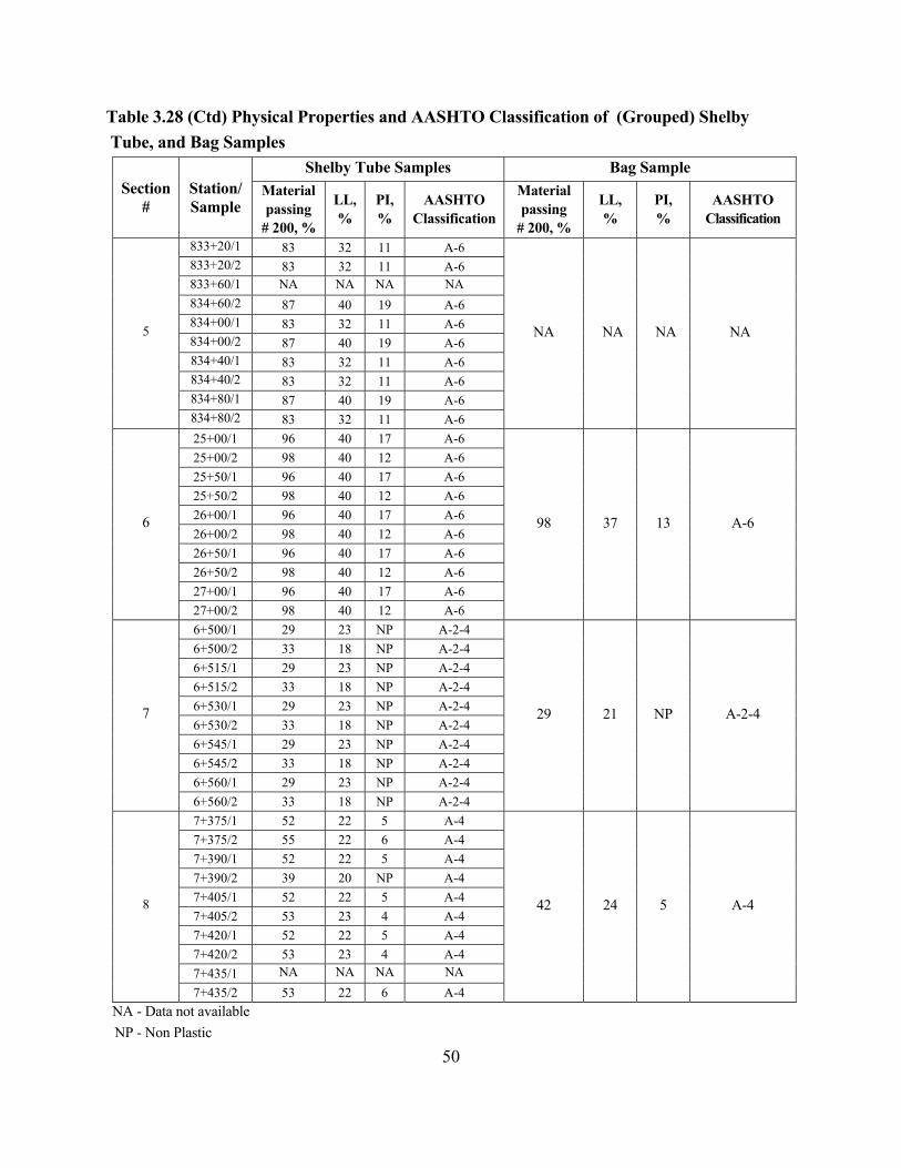
Table 3.28 lists the results of the aforementioned tests for all of the samples from the ten sections
included in the study.
3.2.5.2 Routine Laboratory Tests on Bag Samples
In order to double-check the soil classification based on Shelby tube samples, a bag
sample from each section was subjected to particle size analysis (AASHTO T88-90), Atterberg
limits (AASHTO T89-90 and T90-87), and Standard Proctor test (AASHTO T99-90).
Table 3.28 lists the results of those tests for all of the ten sections. These tests were intended to
establish benchmark properties of the soils being studied. As reported, each Shelby tube sample,
after being tested for resilient modulus, was subjected to classification tests. Comparison of
those results with the bag sample properties enabled us to assess the (natural) spatial variability
in each section.
Besides classification tests, 2.8 in. by 5.6 in. (71 mm by 142 mm) samples (three for each
section) were reconstituted at the respective optimum moisture and maximum density and tested
49
Table 3.28 Physical Properties and AASHTO Classification of (Grouped) Shelby Tube, and Bag Samples
Shelby Tube Samples Bag Sample Section
# Station/ Sample
Material passing
# 200, %
LL, %
PI, %
AASHTO Classification
Material passing
# 200, %
LL, %
PI, %
AASHTO Classification
852+50/1 47 29 11 A6 852+50/2 NA NA NA NA853+00/1 NA NA NA NA853+00/2 NA NA NA NA853+50/1 47 29 11 A6 853+50/2 NA NA NA NA853+75/1 47 29 11 A6 853+75/2 NA NA NA NA854+00/1 56 25 15 A6
1
854+00/2 NA NA NA NA
55
22
6
A-4
54+00/1 NA NA NA NA54+00/2 NA NA NA NA55+00/1 31 20 NP A-2-4 55+00/2 NA NA NA NA56+00/1 31 20 NP A-2-4 56+00/2 NA NA NA NA57+50/1 31 20 NP A-2-4 57+50/2 91 54 23 A-7-6 58+50/1 48 27 8 A-2-4
subgrade surface 4.3 1 9000 lb wheel load over 18 in. pavement 18 in. below
subgrade surface 4 1.3
6 in. below subgrade surface 14.6 2.6
2500 lb load on 12 in. FWD plate 18 in. below
subgrade surface 4.4 0.6
6 in. below subgrade surface 8.5 2.5
2500 lb load on 18 in. FWD plate 18 in. below
subgrade surface 4 0.7
1 psi = 6.89 kPa 1in. = 25.4 mm
the subgrade. The stress states calculated at various depths, employing KENLAYER, are
tabulated in Table 4.3. Stress states at 6 in. and 18 in. depths, including overburden, were
subsequently employed in resilient moduli computation of Shelby tube samples retrieved from
corresponding depths. The results in entirety are not presented in the report for brevity;
however, the resilient moduli of first sample (0 to 12 in.) and second sample (12 to 24 in.)
employing, respectively, the two stess scenarios (stresses σ1 = 8.5 psi, σ3 = 2.5 psi and σ1 = 4.0
psi, σ3 = 0.7 psi) are presented in Table 4.4.
Comparing the two sets, it is noted that the second sample (under the corresponding load
stresses, column 4) appears significantly softer than the first sample, as evidenced by its lower
modulus. The percentage reduction varies from 14% in section #3 to 50% in section 7. Some of
this decrease in MR could be attributed to the lower bulk stress and/or confining stress employed
in calculating the second sample moduli. Also, the moisture content of the second sample is invariably
66
Table 4.4 Resilient Modulus Calculated Employing Two Stress States at Depths 6 in. Below and 18 in. Below Surface, Respectively. Load 2500 lb on 18-in. Plate
Resilient Modulus, psi Section # Station Stress State σ1 = 8.5, σ2 = σ3 = 2.5
First sample Stress State σ1 = 4, σ2 = σ3 = 0.7
Second sample 854 + 00 7711 NAa 853 + 75 11687 NA 853 + 50 12528 NA
1
852 + 50 9866 NA 54 + 00 NA NA 55 + 00 15880 NA 56 + 00 7998 NA 57 + 50 15407 8608
Table 4.4 (Ctd) Resilient Modulus Calculated Employing Two Stress States at Depths 6 in. Below and 18 in. Below Surface, Respectively. Load 2500 lb on 18-in. Plate
NA - Data not available 1 psi = 6.89 kPa Table 4.5 Comparison of Average Density and Moisture of First Sample (0 - 12 in. depth) and Second Sample (12 - 24 in. depth) Shelby Tube
significantly larger, as can be seen in Table 4.6.
Explanation of the selection of stress state for MR calculation follows: First, the 2500-lb
load, is appropriate because the four FWD load levels employed in the test program bracket the
2500-lb load. Second, it is gratifying to note that this load results in stresses, typically sustained
by subgrades (namely, σ1 = 8.5 psi and σ3 = 2.5 psi). Accordingly, modulus values from column
3 of Table 4.4 are chosen to relate to FWD-modulus from Tables 3.6 to 3.15.
4.6 FWD PLATE DIMENSION AND SENSOR TIP SIZE FOR SUBGRADE TEST
4.6.1 General
FWD deflection tests were conducted on ten test sections with two variations from the
normal set up, namely, an 18-in. (450-mm) plate and a modified 16-mm sensor tip (see Table
3.2). The purpose of this investigation was to investigate whether the 18-in. plate (300-mm)
would have advantage over the 12-in. (450-mm) plate and also whether large sensor tips (16
mm) would work better than the standard 10-mm tips.
69
4.6.2 Comparison of Moduli from 18-in. (450-mm) and 12-in. (300-mm) Plates
Average moduli of nine test stations in each section, for each sensor, are presented in the
last row of Tables 3.6 to 3.15 and 3.16 to 3.24, respectively, for the large and small plates. The
first question is: Are they statistically equal? A Mann-Whitney-Wilcoxon test for comparison of
two independent variables (50) was performed to test the difference between the first sensor
modulus (E1) obtained from the large and the small plates. The same comparison test was
performed on the offset sensor E3-5 (average of third, fourth and fifth sensors) and both of the
results are tabulated in Table 4.7. Evidence is lacking to suggest that plate size has any effect on
E1 and E3-5.
Coefficient of Variation (COV) of E1 of both plates is listed in columns 2 and 3 while
COV of E3-5 in columns 4 and 5 of Table 4.8. It is noted that E1 values from the large plate show
large variations within a section, as signified by larger COV values. It could be that uneven
seating of large plate adversely affects E1. Unpredictable plate vibration could be another
reason. The COV of the offset sensors (E3-5) with large plate, however, is improved compared to
that for the small plate results.
The side-by-side tests with two plates revealed another compelling result that the first
sensor moduli indeed shows a large variation regardless of the size of the plate, as can be seen in
Figure 4.2, for a typical section (#8). Normalized deflections (deflection per unit load) of sensor
1 shows significant variation compared to those of sensor 4. Some 36 sensor 4 data points
bunch together right on the equality line, whereas the, corresponding points for the first sensor
deflections, hardly show any trend. Also, the theoretical result that first sensor deflections of 12-
in. and 18-in. plates conform to a ratio of 1·5 is not satisfied. More than plate size, sensor
position affects the precision of deflection results.
70
Table 4.7 Summary of Statistical Test Results Comparing 18-in. (450-mm) Plate Modulus to 12-in. (300-mm) Plate Modulus
Average E1, psi Average E3-5, psi Section
# 18-in. Plate
12-in. Plate
Mann-Whitney-Wilcoxon Test
Comparing 12- and 18-in. Plate
Moduli, E1
18-in. Plate
12-in. Plate
Mann-Whitney-Wicoxon Test Comparing
12- and 18-in. plate Moduli, E3-5
1 3240 NA NA 14410 NA NA 2 10570 10630 No difference 13660 13130 No difference 3 8060 7870 No difference 18100 23170 Different 4 13400 15770 No difference 27360 26500 No difference 5 16920 17710 No difference 31000 30330 No difference 6 12690 15130 No difference 19460 20500 No difference 7 24770 32710 Different 26240 27380 No difference 8 25380 31290 No difference 25850 28670 No difference 9 28310 33480 No difference 29800 29500 No difference
10 7620 9040 No difference 7510 6650 No difference
NA - Data not available 1 psi = 6.89 kPa Table 4.8 Comparison of Coefficient of Variation of 12-in. and 18-in. Plate Moduli
Coefficient of Variation, percent E1 E3-5 Section #
The resilient modulus predicted by linear relation is in good agreement with the
laboratory MR. Despite good predictions, the relation violates a necessary physical boundary
condition that both moduli should approach zero identically. Instead, with the first sensor elastic
modulus zero, a resilient modulus in excess of 10,000 psi (70 MPa) is predicted. In soft soils,
therefore, this resilient modulus prediction is suspect. The viability of linear model is
questionable, because of its inability to make reasonable MR predictions for a range of soils.
As indicated at the outset, the one-to-one relation predicts reasonable design resilient
modulus, should the subgrade tested be homogeneous and moderately stiff. Due in part to the
top stiff surface layer perhaps, the resilient moduli of sections #3, and #9 are overpredicted.
While testing a subgrade with a soft layer overlying a stiff layer, as in section #4, the resilient
modulus is underpredicted, however, (20,040 psi (138 MPa) vs. 12,780 psi (88 MPa)). With a
soft top layer why section #1 departed from under-prediction is still not clear. These differences
in resilient moduli arise from the fact that the overall response under the FWD test and the TP46
test happen to be different, attributable to the non-homogeneity of the subgrade and nonlinearity
of soil. To summarize, though a one-to-one relation is preferred for its simplicity, when
implementing that relationship in low stiffness soils, the resilient modulus prediction becomes ad
hoc for the reason that E1 needs to be replaced by E3-5. Replacing E1 by E3-5 can give rise to
overprediction of resilient moduli, as we note in sections #1 and #3. One also has to contend
with the likelihood of overprediction of resilient modulus in stiff soils.
Compared to linear and one-to-one relations, the power relation makes fewer assumptions
in predicting design resilient modulus from FWD elastic modulus, E1 and E3-5. Employing E1
and E3-5, resilient modulus values are computed and the lesser of the two is selected as the design
value. Relying on both E1 and E3-5 in predicting a representative resilient modulus is desirable
94
for the following reasons: First, the subgrade can seldom be homogeneous. In soft soils or soft
soil atop a stiff soil, E1 is generally smaller than E3-5. However, if the soil deposit is stiff, despite
possible layering (that is, slight variations in stiffness with depth), E1 tends to be comparable to
E3-5. Realizing that E1 and E3-5 are affected by layering, which seldom is known during FWD
test, an argument may be made in employing both E1 and E3-5. Should the two MR values be
different, the lesser of the two is selected, resulting in a conservative design. Note, no ad hoc
assumptions are introduced in selecting a probable resilient modulus for the subgrade, and finally
the design modulus. Second, in high stiffness soils, the resilient modulus is not over predicted.
The leveling off of the E1 vs. MR curve ensures that high FWD elastic moduli do not result in
large predicted MR values. The fact that the two curves cross over at approximately 35,000 psi
(241 MPa) beyond which E1 surpassing E3-5 agrees with our field results. A stiff or stiff atop a
soft soil resulting in E1 equal to or larger than E3-5 is a relevant finding in this regard. Typical
examples being sections #7, #8 and #9, where E1 is close to E3-5, though not slightly larger.
Third, this method gives better correlation than that of one-to-one relation and as good a
correlation as linear method as indicated by the R-squared values (Figures 4.8, 4.10 and 4.15).
In addition, it satisfies the intuitive physical condition as well. This method where E1 and E3-5
are both contributing to the selection of design resilient modulus is by far our recommendation.
4.10 DATA ANALYSIS SOFTWARE
The task at hand in determining a design resilient modulus for new pavement design
starts with FWD tests followed by an analysis of deflection data. Each subgrade section tested
may show substantial spatial variation in response (deflection) and, in turn, modulus, so that the
section in question may, in effect, comprise one or more uniform sections or homogeneous units.
A software program to perform these two tasks--namely, data reduction and subsectioning, if
95
warranted--is developed as a part of this study, the details of which can be seen in Chapter 5.
This program, following the calculation of elastic modulus from FWD deflection data, estimates
station-by-station resilient modulus utilizing elastic modulus. With the resilient modulus, we
employ cumulative difference approach technique (2) for testing and delineating homogeneous
units for the subgrade in question. By way of output, the program prints out the length of each
uniform section, the mean and standard deviation of design resilient modulus for each uniform
section, and a resilient modulus of each station plotted with distance along the road.
4.11 SUMMARY
With the objective of correlating FWD-based elastic modulus with resilient modulus
from TP46 results, the two sets of data obtained from nine test sections are scrutinized ensuring
that the data is reasonable in view of the unique nature of (for example, layering) each subgrade
section. Whether the sampling (by Shelby tube) has any effect on resilient modulus test results is
discussed. A side-by-side test with two plate sizes and two sensor tip sizes led us to select an 18-
in. plate and standard 10 mm tip for subgrade investigation. In selecting the appropriate resilient
modulus value, the stress dependency of modulus is taken into account. After a discussion of
elastic modulus computed from seven deflection sensors, a decision has been made to use both
E1 (first sensor modulus) and the offset sensor modulus E3-5 (average of third, fourth, and fifth
sensor modulus), seeking independent correlations with MR.
Of the three procedures described to estimate probable resilient modulus for a test station,
the recommended procedure employs both E1 and E3-5 sequentially, choosing the lesser resilient
modulus for design purpose. A software program titled FWDSUBGRADE, developed as a part
of this study, performs all of the calculations, and identifies subsections, if any, in the section in
question. A detailed discussion of this program will be presented in Chapter 5.
96
CHAPTER 5
PLANNING FWD TEST AND CALCULATION OF DESIGN RESILIENT MODULUS
5.1 OVERVIEW
A methodology for choosing a design resilient modulus, relying on FWD test deflections
and corresponding elastic modulus, has been the topic of Chapter 4. Planning FWD test and
collecting field data is an important component that supports this methodology. A brief
description of FWD test configuration and advance field preparation will be covered in the first
part of the chapter. Each subgrade project under consideration may be a fraction of a mile or a
few miles in length. Inherent spatial variation along the road shall be recognized. And, if the
variation of modulus is statistically significant, the project should be divided into subsections or
homogeneous units, as described in the second part of this chapter. Included in the third part of
this chapter is a brief description of the exclusive computer program, FWDSUBGRADE, for
arriving at homogeneous unit(s), if warranted.
5.2 PLANNING FWD TEST IN THE FIELD
The field test shall be planned with extreme care ensuring that data collected from FWD
tests be minimally affected by spatial variations in the field. The planning of the field test
includes the following:
1. Equipment selection
2. When and where to test?
3. Validation of deflection data
Data collected during the FWD test include the load applied and the resulting peak sensor
deflections. A validation procedure of deflection data is included in section 3.2.1 and is
97
implemented in the computer program described in the latter part of this chapter. It entails
checking each deflection basin for negative slopes. That is, the sensor deflection shall not
increase as the sensor distance from the load center increases.
5.2.1 Equipment Selection
A FWD with a seven-sensor configuration shall be used for the field deflection study. A
load package inducing a load of 2,500 ± 100 pounds is recommended. An 18-in. (450-mm) load
plate is preferred for subgrade testing. The velocity sensor spacing shall be adjusted such that
they are positioned with one at the center of the load plate and the remaining six sensors at 12 in.
(305 mm) 18 in. (457 mm), 24 in. (610 mm), 36 in. (914 mm), 48 in. (1219 mm), and 60 in.
(1524 mm), respectively, from the center of the plate.
5.2.1.1 Test Procedure
At each station two seating loads followed by three or more load drops of 2,500 ± pounds
shall be applied. The peak load and peak deflection of each sensor (total of seven sensors) shall
be monitored and recorded, with the data collection repeated for all of the load repetitions
(except for the two seating loads). Tests shall be repeated at constant intervals (or uniform
spacing) along the road till the end of the proposed subgrade. Because FWDSUBGRADE
software does not use the beginning station modulus, it shall not be tested; however, the last
station (or the project end) must be tested, regardless if the last section is equal to or smaller than
the predetermined interval. Though the test interval (spacing) is left to the discretion of the
project engineer, based on the precision required and practicality, a test interval of 50 ft. (15 m)
is recommended.
98
5.2.2 When and Where to Test?
Subgrade soil, though compacted to specified density and moisture, could become soft
should it absorb excessive moisture resulting from precipitation for an extended period of time.
Likewise, it could become hard if the soil becomes dry, as can be expected during a long
drought. Additionally, some coarse-grain soils could lose strength when subject to extreme
drought. For these reasons, it is important to schedule FWD testing when the moisture of the
subgrade is close to optimum moisture. Approximately, the moisture during tests shall be within
the upper limit of optimum moisture +2 percent, and the lower limit of 75 percent of optimum.
Test locations along the road shall be so chosen as to avoid loose surface material and
wheel ruts due to construction traffic. Uneven subgrade surface could result in load plate not
being seated properly giving rise to asymmetrical stress distribution affecting sensor deflections.
Loose surface material also affects the sensor deflections. Experience suggests that loose
particulate material shifts while the load is being dropped. Figure 4.4 is an illustration of a
sensor imprint where coarse loose particles congregate around the sensor tip, caused primarily by
vibration due to impacting load. If subgrade to be tested is uneven and/or rutted, it shall be
bladed and lightly recompacted before FWD testing to ensure a reasonably smooth surface for
proper seating of the plate, and the sensors, as well. Finally, test locations shall be aligned such
that they are within 10 ft. of the centerline of the paved surface for 14 ft. wide lanes or 8 ft. for
12 ft. wide lanes.
5.3 SELECTION OF DESIGN UNIT
When considering a reasonably large pavement project, deflections along the prepared
subgrade and, in turn, the moduli could experience changes of large magnitude signaling
statistically different units within a given project. Frequently, the engineer must rely on the
99
analysis of a measured pavement response variable (e.g., modulus) for unit delineation. The
designer could develop a plot of the measured response variable as a function of the distance
along the project. This can be done manually or through computerized data analysis-graphic
systems. To illustrate the approach, the problem of sectioning a highway based on friction
Figure 5.1 FN(40) Results versus Distance Along Project (Adapted From Reference 2)
number (FN (40)) is included herein. Figure 5.1 is a plot of friction number results, FN (40),
versus station number along an actual highway system. The proposed methodology is adopted
from reference 2.
Once the plot of a pavement response variable has been generated, it may be used to
delineate units through several methods. The simplest of these is visual examination to
subjectively determine where relatively unique units occur. In addition, several analytical
100
methods are available to help delineate units, with the recommended procedure being the
“cumulative difference.” This analytical procedure, readily adaptable to computerized
evaluation, relies on the simple mathematical fact that when the variable Zc (defined as the
difference between the area under the response curve at any distance and the total area developed
from the overall project average response at the same distance) is plotted as a function of
distance along the project, unit boundaries occur at the location where the slopes (Zc vs distance)
change sign. Figure 5.2 is a plot of the cumulative difference variable (Zc) for the data shown in
Figure 5.1. For this example, 11 preliminary analysis units are defined. The engineer must then
evaluate the resulting length of each unit to determine whether two or more units should be
combined for practical construction considerations and economic reasons. The combination of
units should be done relative to the sensitivity of the mean response values for each unit upon
performance of future designs.
5.4 COMPUTER PROGRAM, FWDSUBGRADE, TO CALCULATE DESIGN
MODULUS
As alluded to before, the program, FWDSUBGRADE, performs two major tasks in
arriving at a design modulus. First, accepting deflection data, it calculates elastic modulus and,
in turn, derives resilient modulus of soil at each station. Employing these station-by-station
moduli in an analytical procedure known as cumulative difference, the program delineates
homogeneous units, outputting the length of each unit (in the event of identifying multiple units)
and the corresponding resilient moduli – both mean and standard deviation –which shall form the
design resilient moduli. The logic of these operations is presented in the flow chart in
Figure 5.3. Detailed operations of the program can be seen in Appendix D.
101
Note the output of the program includes a plot of the resilient modulus at each station as a
function of distance along the project. This plot should serve as a guide in combining adjacent
units to form “design units.” Practical construction considerations and economic reasons likely
Figure 5.2 Delineating Analysis Units by Cumulative Difference Approach (Adapted From Reference 2)
govern these decisions. For example, should there be short sections of relatively soft
material,they shall be upgraded with additives (cement, lime, lime-fly ash, etc.) to facilitate
merger with contiguous homogeneous units.
5.5 SUMMARY
Planning the FWD test in the field, including equipment selection and site preparation for
subgrade deflection measurements, is described. Test specifics, for example, seating load and
102
repetitions required, are also a part of this discussion. With the calculated modulus response in
each project, a methodology for unit delineation is presented. Finally, a flow chart outlining the
operations necessary to accept FWD deflection data and to output homogeneous units (with
boundaries identified) and corresponding design modulus constitute the last section of this
chapter.
103
i = i + 1
Figure 5.3 Flow Chart of Program FWDSUBGRADE
Start
Input data
Read data from FWD file (i = 1,n)
Check deflections (Dj>Dj+1), j = 1 to 7, Criteria not satisfied then set both to zero
Calculate elastic modulus (E1 to E7), j = 1 to 7, If Dj = 0 then Ej = 0 and if Ej > 35,000 psi then Ej = 35,000
Calculate E3-5av (average elastic modulus of E3, E4 and E5)
Calculate MR1 and MR3-5 from E1 and E3-5av, Choose lower of the two (MR) values
Read stations along with MR values excluding stations with MR = 0, Run unit delineation test and calculate
length of sections along with starting and ending stations, Section mean & standard deviation, Graph of MR vs. stations
Save and print results
End
104
CHAPTER 6
SUMMARY AND CONCLUSIONS
6.1 SUMMARY
This project addresses the issue of employing a FWD test for subgrade characterization.
A research program, including field and laboratory tests, is initiated seeking a relation between
deflection-based elastic modulus, E, and laboratory resilient modulus, MR. Ten as-built subgrade
sections were tested using the FWD followed by the Dynamic Cone Penetrometer to detect soil
layering, if any. Undisturbed soil samples were retrieved utilizing a thin wall Shelby tube and
tested in the laboratory employing TP46 protocol. Elastic modulus calculations employing
forward calculation equations (assuming an elastic half-space) was regressed against laboratory
resilient modulus, advancing various approaches (models) for MR prediction. A feature of the
chosen approach is that both center sensor modulus and offset sensor moduli enter in the process
independently resulting in two equations. With two equations, two resilient moduli can be
derived, and the lesser of the two yield a conservative value for design. Having been derived
with multiple sensor moduli, it promises to be a viable method for subgrade characterization,
especially when sizeable nonhomogeneity is expected in built-up subgrades. A short-cut
procedure suggesting a one-to-one relation between E1 and MR is also presented, where, for the
two extreme reaches (lower and upper), E1 is replaced by E3-5 when E1 < 9000 psi, and lesser of
E1 and E3-5 when E1 > 25,000 psi.
An exclusive program, FWDSUBGRADE, was developed to analyze FWD deflection
data obtained from subgrade tests, extracting the first sensor modulus E1, and average of three
offset sensors, E3-5. Employing E1 and E3-5, two distinct resilient moduli are derived with the
105
lesser of the two serving as the design resilient modulus. The program, in addition to calculating
station-by-station resilient modulus, relying on what is known as cumulative difference
technique, delineates homogeneous units of the subgrade, outputting mean and standard
deviation of resilient modulus for each homogenous section. A graphical plot of resilient
modulus at each station along the project is another output of the program.
6.2 CONCLUSIONS
The analysis of test results focused on relating FWD elastic modulus to resilient modulus
of undisturbed Shelby tube samples and recommending this model for estimating a design
resilient modulus. Summarized herein are the major conclusions/observations, related to test set-
up, modulus results and data analysis:
1. FWD is a viable test device for testing subgrade soil provided the stress in the subgrade
can be kept low, ensuring elastic behavior (a 2,500 ± lb load on an 18-in. plate meets the
stress criteria).
2. The first sensor deflection exhibits large variability compared to those of the offset
sensors, except the second sensor deflection that also shows large fluctuation especially
with an 18-in. plate.
3. The standard 10 mm sensor tip performed as satisfactorily as the larger tip, 16 mm size.
4. Forward calculation employing elastic equations is found to result in consistent elastic
moduli values from all of the offset sensor deflections except sensor 2.
5. The first sensor modulus tends to be lower than each of the offset sensor modulus when
the surface material is softer than the underlying soil, while the first sensor modulus is
either e qual to or slightly larger than the offset sensor modulus when the subgrade is
uniformly stiff or a stiff material overlies a softer material.
106
6. Disturbance caused by pushing the Shelby tube sampler into a desiccated top layer
resulted in re-compaction of samples, and, in turn, increased resilient modulus values.
Moisture also influenced the resilient modulus results.
7. Though tested at appointed stresses, resilient modulus based on TP46 protocol exhibits
stress dependency, warranting the use of universal model to adjust the resilient modulus
values with respect to stress state.
8. Field, as well as laboratory test results, show that subgrade in all of the test sections is
non-uniform, with more variation spatially than in the vertical direction.
9. Though the data revealed a one-to-one relationship between E1 and MR for a limited
range of moduli values, the relation is not robust enough nor could be justified on a
theoretical basis.
10. Neither first sensor modulus nor offset sensor moduli (E3-5: average of third, fourth and
fifth sensor moduli) could independently capture subgrade response characteristic,
therefore, employing E1 and E3-5 concurrently, two resilient modulus values are chosen.
Lesser of the two values constitutes the design resilient modulus.
6.3 RECOMMENDATIONS FOR FURTHER RESEARCH
This research has charted a viable procedure for characterizing subgrade employing
FWD, a device that has been used for some time for pavement evaluation including the in-place
subgrade. In the overall pavement evaluation scheme, the nonhomogeneity of subgrade plays a
minor role as compared to when a subgrade is being tested directly on the surface. In order to
account for the nonhomogeneity only, both center sensor and offset sensor moduli have been
brought into prominence in choosing the appropriate design resilient modulus. Now the two
relationships/equations derived in this research needs to be continually refined as more field test
107
data becomes available. More test data on relatively soft soils, whose modulus falls below
10,000 psi (70 MPa), would indeed improve the robustness of the two relations, that form the
backbone of the correlation methodology.
Also studies are encouraged to map out the change in subgrade moduli, as other layers,
for example, subbase/base and surface, are emplaced over the subgrade. This would help to
substantiate the 0.33 factor for translating subgrade FWD modulus (backcalculated), to resilient
modulus in the context of pavement evaluation.
6.4 IMPLEMENTATION
The subgrade soils selected for this study covered a wide variety of Mississippi soil
types, plasticity indices, and gradations. Accordingly, the procedures described for determining
design MR-values using the FWD shall be widely applicable, at least for unbound, fine-grain
subgrade soils. Design resilient modulus may be calculated employing equations in Figure 4.15
followed by a plot similar to that in Figure 5.1, in choosing homogeneous sections. Alternately,
the computer program FWDSUBGRADE performs all of the above steps.
The entire procedure of reading the FWD data in real time and making calculations,
outputting homogeneous units with mean and standard deviation of resilient modulus, is
programmed and furnished for ready-use by MDOT. The ability to perform real time data
analysis in the field enables the engineer to verify the accuracy of sub-sectioning and to some
extent validate the resilient modulus values predicted by the analysis procedure.
6.5 BENEFITS
The principle benefit of the correlations developed in this research resides in being able
to use FWD for subgrade characterization. Subgrade resilient modulus for pavement design (in
accordance with AASHTO Guide and the 2002 Guide) can now be determined employing
108
relationships developed in this study. FWD deflection-based characterization is preferred
primarily for two reasons: (i) in-situ tests circumvent disturbance (recompaction/decompaction)
affecting the test outcome, and (ii) in-situ tests simulate the stress state in the material better than
that can be attained in TP46 test, for example. With the results accomplished in this research
incorporated in a user-friendly program, feasibility of the FWD test directly on subgrade is
indeed enhanced.
Recognition of spatial variability of soil compaction uncovered in this study could lead to
better construction control specifications, in terms of employing statistical quality control. As
FWD is extensively used in pavement evaluation, receiving widespread recognition, its use in
subgrade evaluation is a logical choice and is likely to be embraced by pavement engineers.
109
REFERENCES
1. Witczak, M., Qi, X. and Mirza, M.W., “Use of Nonlinear Subgrade Modulus in AASHTO Design Procedure”, ASCE Journal of Transportation Engineering, Vol. 121, No. 3, 1995, pp. 273-282.
2. AASHTO Guide for Design of Pavement Structures 1993. AASHTO, Washington, DC,
1993. 3. Heukelom, W., and Klomp, A.J.G., “Dynamic Testing as a Means of Controlling
Pavements During and After Construction”, Proceedings of the First International Conference on Structural Design of Asphalt Pavements, University of Michigan, 1962.
4. Hassan, A., “The Effect of Material Parameters on Dynamic Cone Penetrometer Results
For Fine-grained Soils and Granular Materials”, Ph.D. Dissertation, Oklahoma State University, Stillwater, Oklahoma, 1996.
5. Burnham, T., and Johnson, D., “In-Situ Characterization Using the Dynamic Cone
Penetrometer”, Report MN-93/05, Minnesota Department of Transportation, Maplewood, Minnesota, 1993.
6. Chai, G., and Roslie, N., “The Structural Response and Behavior Prediction of Subgrade
Soils Using Falling Weight Deflectometer in Pavement Construction”, Proceedings, Third International Conference on Road & Airfield Pavement Technology, Beijing, China, April 1998.
7. George, K.P. and Uddin, W., “Subgrade Characterization for Highway Pavement
Design”, Final Report, Submitted to Mississippi Department of Transportation, The University of Mississippi, December 2000.
8. Ali, N.A., and Khosla, N.P., “Determination of Layer Moduli Using a Falling Weight
Deflectometer”, Transportation Research Record 1117, TRB, National Research Council, Washington, D.C., 1987, pp. 1-10.
9. Newcomb, D.E., “Comparison of Field and Laboratory Estimated Resilient Moduli of
Pavement Materials”, Asphalt Paving Technology, Association of Asphalt Paving Technologists, Vol. 56, February 1987, pp. 91-106.
10. Von Quintus, H.L., and Killingsworth, B.M., “Comparison of Laboratory and In-Situ
Determined Elastic Moduli”, A paper presented at the 76th Annual Meeting of the Transportation Research Board, Washington, D.C., January 1998.
11. Chen, Bilyeu, and He, “Comparison of Resilient Moduli Between Field and Laboratory
Testing: A Case Study”, A Paper Presented at the 76th Annual Meeting of the Transportation Research Board, Washington, D.C., January 1998.
110
12. Houston, W.N., Mamlouk, M.S., and Perera, R.W.S., “Laboratory versus Nondestructive Testing for Pavement Design”, ASCE Journal of Transportation Engineering, Vol. 118, No. 2, 1992, pp. 207-222.
13. Van Deusan, D.A., Lenngren, C.A., and Newcomb, D.E., “A Comparison of Laboratory
and Field Subgrade Moduli at the Minnesota Road Research Project”, Nondestructive Testing of Pavements and Backcalculation of Moduli, ASTM STP 1198, H.L. Von Quintus et al., eds., ASTM, 1994.
14. Nassar, W., Al-Qadi, I., Flinlsch, G.W., and Appea, A., “Evaluation of Pavement Layer
Response at the Virginia Smart Road”, Virginia Polytechnic Institute, Blacksburg, VA, 1990.
15. Rahim, A., and George, K.P. “Falling Weight Deflectometer for Estimating Subgrade
16. Seeds, S.B., Ott, W.C., Milchail, M., and Mactutis, J.A. “Evaluation of Laboratory
Determined and Nondestructive Test Based Resilient Modulus Values From WesTrack Experiment”, Nondestructive Testing of Pavements and Backcalculation of Moduli ASTM STP 1375, S. Tayabji and O. Lukanen eds., ASTM, 2000.
Characterization of Subgrade Soils and Granular Base Materials at the Minnesota Road Research Project”, Report No. MN/RC-96/19, Minnesota Department of Transportatino, St. Paul, Minnesota, December 1995.
18. Newcomb, D.E. and Birgisson, B., “Measuring In-Situ Mechanical Properties of
19. Gros, C., “Use of a Portable Falling Weight Deflectometer: Loadman”, University of
Oulu, Publications of Road and Transportation Laboratory, No. 20, 1993. 20. Kudla, W., Floss, R., and Trautmann, C., “Dynamic Plate Compression Test - Rapid
Testing Method for Quality Assurance of Unbound Course”, Autobahn 42, No. 2. (Published in German), 1991.
21. Rogers, C.D.F., Brown, A.J. and Fleming, P.R., “Elastic Stiffness Measurement of
Pavement Foundation Layers”, Unbound Aggregates in Roads 4, Edited by Dawson A. and Jones R.H., Nottingham University, 1995.
22. Hou, T.Y., “Evaluation of Layered Material Properties from Measured Surface
Deflections”, Ph.D. Thesis, University of Utah, Salt Lake City, Utah, 1977.
111
23. Harichandran, R.S., Mahmood, T., Raab, A.R., and Baladi, G.Y., “Modified Newton Algorithm for Backcalculation of Pavement Layer Properties”, Transportation Research Record 1384, TRB, National Research Council, Washington, D.C., 1993, pp. 15-22.
24. Odemark, N., “Undersokning av elasticitetegenskaperna hos olika jordarter samt terori
for berakning av belagningar eligt elasticitesteorin”, Statens Vaginstitute, meddelande 77, 1949.
25. Ullidtz, Per, “Will Nonlinear Backcalculation Help?” Nondestructive Testing of
Pavements and Backcalculation of Moduli, Volume 3, ASTM STP 1375, S. Tayabj and E.D. Lukanen, eds., ASTM, 2000.
26. Lee, S.W., Backcalculation of Pavement Moduli by Use of Pavement Surface
Deflections, Ph.D. dissertation, University of Washington, Seattle, Washington, 1988. 27. Irwin, L.H., User’s Guide to MODCOMP 2, Version 2.4, Report No. 83-8, Cornell Local
Roads Program, Cornell University, Ithaca, N.Y., November 1983. 28. Van Cauwelaert, F.J., Alexander, D.R., White, T.D. and Barker, W.R. “Multilayer Elastic
Program for Backcalculating Layer Moduli in Pavement Evaluation”, Nondestructive Testing of Pavements and Backcalculation of Moduli, ASTM STP 1026, A.J. Bush III and Gilbert Baladi, eds., American Society for Testing and Materials, Philadelphia, PA, 1989.
29. Uzan, J., et al., A Microcomputer Based Procedure for Backcalculating Layer Moduli
from FWD Data, Research Report No. 1123-1, Texas Transportation Institute, College Station, TX, September 1988.
30. Haiping, Z., Hicks, R.G. and Bell, C.A. “BOUSDEF: A Backcalculation Program for
Determining Moduli of a Pavement Structure”, Transportation Research Record 1260, TRB, National Research Council, Washington, D.C., 1990.
31. Ullidtz, P. and Stubstad, R.N. “Analytical-Empirical Pavement Evaluation Using the
Falling Weight Deflectometer”, Transportation Research Record 1022, TRB, National Research Council, Washington, D.C., 1985.
32. Moossazadeh, J.M. and Witczak, W. “Prediction of Subgrade Moduli for Soil That
Exhibits Nonlinear Behavior”, Transportation Research Record 810, TRB, National Research Council, Washington, D.C., 1981.
33. Dunlap, W.S. “A Report On A Mathematical Model Describing the Deformation
Characteristics of Granular Materials”, Technical Report 1, Project 2-8-62-27, TTI, Texas A & M University, 1963.
112
34. Seed, H.B., Mitry, F.G., Monosmith, C.L., and Chan, C.K. “Prediction of Pavement Deflection From Laboratory Repeated Load Tests”, NCHRP Report 35, Transportation Research Board, Washington, D.C., 1967.
35. May, R.W. and Witczak, M.W. “Effective Granular Modulus to Model Pavement
Response”, Transportation Research Record 810, TRB, National Research Council, Washington, D.C., 1981.
36. Uzan, J., “Characterization of Granular Materials”, Transportation Research Record
1022, TRB, National Research Council, Washington, D.C., 1985. 37. Yau, A. and Von Quintus, H.L., “Study of LTPP Laboratory Resilient Modulus Test Data
38. Ni, B., Hopkins, T.C., Sun, L., and Beckham, T.L., “Modeling the Resilient Modulus of
Soils”, Proceedings, Sixth International Conference Bearing Capacity of Roads, Railways and Airfields, Lisbon, Portugal, 2002.
39. Stubstad. R.N., et al., “LTPP Data Analysis: Feasibility of Using FWD Deflection Data
to Characterize Pavement Construction Quality” NCHRP Web Document #52: Project 20-59 (9), Washington, D.C., 2002.
40. Daleiden, J.F., Killingsworth, B.M., Simpson, A.L., and Zamora, R.A., “Analysis of
Procedures for Establishing In Situ Subgrade Moduli”, Transportation Research Record 1462, TRB, National Research Council, Washington, D.C., 1994.
41. Akram, T., Scullion, T., and Smith, R.E., “Comparing Laboratory and Backcalculated
Layer Moduli on Instrumented Pavement Sections”, Special Technical Publication (STP) 1198, ASTM, Philadelphia, PA, 1994.
42. Nazarian, S., Yuan, D., and Baker, M.R. “Rapid Determination of Pavement Moduli
With Spectral-Analysis-of-Surface-Waves Method”, Research Record 1243-1F, Center for Geotechnical and Highway Materials Research, University of Texas at El Paso, 1995.
43. Von Quintus, H. and Killingsworth, B., “Design Pamphlet for the Backcalculation of
Pavement Layer Moduli in Support of the 1993 AASHTO Guide for the Design of Pavement Structures”, Report No. FHWA-RD-97-076, FHWA, USDOT, Washington, D.C., 1997.
44. Shahid, M.A., Thom, N.H., and Fleming, P.R. “In Situ Assessment of Road
Foundations”, Journal of the Institute of Highways and Transportation and IHIE, Vol. 44, No. 11, 1997.
113
45. Fleming, P.R., “Small-scale Dynamic Devices for the Measurement of Elastic Stiffness Modulus on Pavement Foundations”, Nondestructive Testing of Pavements and Backcalculation of Moduli: ASTM STP 1375, S. Tayabji and O. Lukanen, eds., ASTM, 2000.
46. Cooleman, H.W. and Steele, W.G. “Experimentation and Uncertainty Analysis for
Engineers”, John Wiley & Sons, Inc., New York, N.Y., 1989. 47. Harr, M.E., “Mechanics of Particulate Media”, McGraw-Hill, New York, N.Y., 1977. 48. “Humboldt Stiffness Gauge, A Field Instrument for Measuring Lift Stiffness and Soil
Modulus” Humboldt Manufacturing Co., Norridge, IL. 49. George, K.P., “Soil-Cement Field Trial” Interim Report to Mississippi Department of
Transportation, University of Mississippi, University, M.S., 2001. 50. Netter, J., Wasserman, W., and Whitmore, G.A. Applied Statistics, Allyn and Bacon,
Inc., 1988.
114
APPENDIX A
FWD DEFLECTION BASINS, TYPICAL STATION FROM EACH
SECTION
115
0
5
10
15
20
25
30
35
40
45
50
0 10 20 30 40 50 60 70Se nsor Dis tance , in.
Def
lect
ions
, mils
1636 lbs2399 lbs3137 lbs4244 lbs
Figure A1 Deflection Basins for Four Loads, Section # 1, Station # 854+25, US 82W, Montgomery County, 18-in. (450-mm) Plate
0
5
10
15
20
25
0 10 20 30 40 50 60 70Se nsor Dis tance , in.
Def
lect
ions
, mils
1599 lbs2276 lbs3002 lbs3949 lbs
Figure A2 Deflection Basins for Four Loads, Section # 2, Station # 56+00, US 61N, Coahoma County, 18-in. (450-mm) Plate
116
0
5
10
15
20
25
30
0 10 20 30 40 50 60 70Sensor Distance, in.
Def
lect
ions
, mils
1636 lbs2374 lbs3076 lbs4170 lbs
Figure A3 Deflection Basins for Four Loads, Section # 3, Station # 152+50, US 61N, Coahoma County, 18-in. (450-mm) Plate
0
5
10
15
20
25
0 10 20 30 40 50 60 70Sensor Distance, in.
Def
lect
ions
, mils
1845 lbs2620 lbs3334 lbs4478 lbs
Figure A4 Deflection Basins for Four Loads, Section # 4, Station # 907+50, US 82W, Montgomery County, 18-in. (450-mm) Plate
117
0
2
4
6
8
10
12
14
16
18
0 10 20 30 40 50 60 70Sensor Distance, in.
Def
lect
ions
, mils
1710 lbs2423 lbs3174 lbs4207 lbs
Figure A5 Deflection Basins for Four Loads, Section # 5, Station # 833+20, US 82W, Montgomery County, 18-in. (450-mm) Plate
0
5
10
15
20
25
0 10 20 30 40 50 60 70Sensor Distance, in.
Def
lect
ions
, mils
1691 lbs2522 lbs3322 lbs4441 lbs
Figure A6 Deflection Basins for Four Loads, Section # 6, Station # 26+50, Norell W, Hinds County, 18-in. (450-mm) Plate
118
0
2
4
6
8
10
12
14
0 10 20 30 40 50 60 70Sensor Distance, in.
Def
lect
ions
, mils
1790 lbs2694 lbs3469 lbs4576 lbs
Figure A7 Deflection Basins for Four Loads, Section # 7, Station # 6+530, US 45N, Wayne County, 18-in. (450-mm) Plate
0
1
2
3
4
5
6
7
0 10 20 30 40 50 60 70Sensor Distance, in.
Def
lect
ions
, mils
1845 lbs2620 lbs3285 lbs4269 lbs
Figure A8 Deflection Basins for Four Loads, Section # 8, Station # 7+405, US 45N, Wayne County, 18-in. (450-mm) Plate
119
0
1
2
3
4
5
6
7
0 10 20 30 40 50 60 70Sensor Distance, in.
Def
lect
ions
, mils
1808 lbs2682 lbs3519 lbs4576 lbs
Figure A9 Deflection Basins for Four Loads, Section # 9, Station # 7+435, US 45N, Wayne County, 18-in. (450-mm) Plate
0
5
10
15
20
25
30
35
0 10 20 30 40 50 60 70Se nsor Dis tance , in.
Def
lect
ions
, mils
1661 lbs2325 lbs2940 lbs4023 lbs
Figure A10 Deflection Basins for Four Loads, Section # 10, Station # 48+50, Nissan W. Parkway, Madison County, 18-in. (450-mm) Plate
120
APPENDIX B
AUTOMATED DYNAMIC CONE PENETROMETER TEST DATA
121
0
200
400
600
800
1000
1200
1400
0 10 20 30 40 50 60 70 80
Number of BlowsPe
netr
atio
n, m
m
852+50
853+50
853+75
854+00
854+50
Figure B1 ADCP Test Results in Section # 1, US 82W, Montgomery County