CMPO Working Paper Series No. 04/101 CMPO is funded by the Leverhulme Trust. Family Income and Educational Attainment: A Review of Approaches and Evidence for Britain Jo Blanden 1 and Paul Gregg 2 1 Centre for Economic Performance, London School of Economics and Department of Economics, University College London 2 Department of Economics, University of Bristol and Centre for Economic Performance, London School of Economics April 2004 Abstract It is widely recognised that, on average, children from poorer backgrounds have worse educational outcomes than their better off peers. There is less evidence on how this relationship has changed over time and, indeed, what exactly leads to these inequalities. In this paper we demonstrate that the correlation between family background (as measured by family income) and educational attainment has been rising between children born in the late 1950s and those born two decades later. The remainder of the paper is spent considering the extent to which these associations are due to the causal effects of income rather than the result of other dimensions of family background. We review the approaches taken to answering this question, drawing mainly in the US literature, and then present our own evidence from the UK, discussing the plausible range for the true impact of income on education. Our results indicate that income has a causal relationship with educational attainment. Keywords: Education, Inequality JEL Classification: JEL I21 I32 Acknowledgements We thank the Leverhulme Trust for funding this research. The authors would like to thank the Sutton Trust for Financial Support. We would also like to thank the editorial board (especially Stephen Machin and Steve Nickell) and an anonymous referee for helpful comments. Andrew Shephard and Alissa Goodman at the Institute for Fiscal Studies were helpful in providing the latest income inequality statistics for families with children. Address for Correspondence [email protected]
Transcript
CMPO Working Paper Series No. 04/101
CMPO is funded by the Leverhulme Trust.
Family Income and Educational Attainment: A Review of
Approaches and Evidence for Britain
Jo Blanden1
and Paul Gregg2
1Centre for Economic Performance, London School of Economics and
Department of Economics, University College London
2Department of Economics, University of Bristol and Centre for Economic Performance, London School of Economics
April 2004
Abstract It is widely recognised that, on average, children from poorer backgrounds have worse educational outcomes than their better off peers. There is less evidence on how this relationship has changed over time and, indeed, what exactly leads to these inequalities. In this paper we demonstrate that the correlation between family background (as measured by family income) and educational attainment has been rising between children born in the late 1950s and those born two decades later. The remainder of the paper is spent considering the extent to which these associations are due to the causal effects of income rather than the result of other dimensions of family background. We review the approaches taken to answering this question, drawing mainly in the US literature, and then present our own evidence from the UK, discussing the plausible range for the true impact of income on education. Our results indicate that income has a causal relationship with educational attainment. Keywords: Education, Inequality JEL Classification: JEL I21 I32
Acknowledgements We thank the Leverhulme Trust for funding this research. The authors would like to thank the Sutton Trust for Financial Support. We would also like to thank the editorial board (especially Stephen Machin and Steve Nickell) and an anonymous referee for helpful comments. Andrew Shephard and Alissa Goodman at the Institute for Fiscal Studies were helpful in providing the latest income inequality statistics for families with children. Address for Correspondence [email protected]
1. Introduction
As income inequality rose after 1980, incomes in households with children fell
relative to those of other households whilst income inequality within this group grew
sharply. The poorest households with children saw virtually no rise in living standards
for twenty years (see Figure 11 and Gregg, Harkness and Machin, 1999, for more
detail).
We know from existing research that children from poorer backgrounds do less well
in a number of dimensions than their peers (see for example Gregg and Machin, 2000)
and in the UK the simple correlation between low income and poor educational
outcomes has been long established (Rowntree, 1901, Glennerster, 1995). In terms of
completed education, children from low-income households go on to leave full-time
education much earlier, and with fewer formal qualifications than their more affluent
counterparts. For example, of children born in 1970, some 26% failed to achieve any
O levels or equivalent by the age of 30, whilst 23% went on to get a degree. Among
children from the poorest 20% of households at age 16, only 11% went on to get a
degree and 41% failed to achieve any O levels. The extent to which the relationship
between low income and poor attainment is causal is, however, less clear.
There is recent evidence that the relationship between family incomes and children’s
outcomes has increased over successive cohorts. Blanden et al. (2002) document that
the intergenerational transmission of income has increased for children born in 1970
(British Cohort Survey) compared with those born in 1958 (National Child
Development Survey). There is also evidence that the increased persistence is in part a
consequence of an increased relationship between family income and educational
attainment. Related papers by Blanden and Machin (2004) and Blanden, Gregg and
Machin (2003) show increased educational inequalities by income group.
The fundamental question is whether it is money itself that makes the difference to
children’s lives and opportunities. If the real drivers of educational outcomes are
1 Gini coefficients for families with children (after adjusting for family size using the McClements scales) are .224 in 1970, .228 in 1980, .320 in 1990, .337 in 1997/98 and .344 in 2002/03 (Institute for Fiscal Studies calculations from the Family Expenditure Survey and Family Resources Survey). It therefore appears that the rise in inequality for families with children was strongest in the 1980s, continued more slowly in the 1990s. Inequality appears to have been steady over the period of the current Labour Government with early increases in equality being offset by more recent reductions perhaps reflecting the impact of the new tax credits after 1999.
2
innate ability, parental education, parenting styles and other factors that are related to,
but not caused by, income then increased income inequality will not matter to
children’s educational attainment. However there are clearly mechanisms by which
income can directly influence attainment such as child care quality, the home
environment, social activities, neighbourhoods and schools. If these are important
then increasing inequality in family income will translate into inequalities in
children’s educational outcomes and their life chances. A clearer understanding of
these issues is key to appreciating the extent to which goals of equality of opportunity
(or meritocracy) can be reconciled with wide income inequalities, and they are
essential to evaluating the educational benefits of reducing child poverty.
Evidence from the UK indicates that low income does have an independent effect on
children’s outcomes after controlling for key aspects of family background and child
ability (see Gregg and Machin, 2000 and Hobcraft, 1998). However, to be confident
that the effect of income has been accurately isolated requires more than controlling
for family background. If unobserved child or family heterogeneity is positively
correlated with income, this will generate an upward bias in the relationship between
income and child attainment. The difficulty of controlling for this heterogeneity
means that the task of separating the influence of income from other aspects of family
background is not straightforward.
The latest research from the US uses a variety of different methods of controlling for
family background and heterogeneity and finds that family income does have a direct
positive effect on educational attainment. However, there is substantia l variation in
the strength of the identified effect (for example see Mayer, 1997, Houston et al.,
2000, Levy and Duncan, 2000, Clark-Kaufman et al. 2003). Our aim in this paper is to
review the evidence on the effect of family income on education and to explore
British data using the same approaches.
We start by presenting a summary of the findings generated by the analysis
undertaken in this paper. Table 1 summarises the results obtained from the different
identification strategies we pursue. We group the results by the survey used. The data
here is taken from two different sources, the BCS 1970 birth cohort and the British
Household Panel Survey, meaning that we are comparing young people who reached
16 in 1986 with those who reached this age in the mid to late 1990s.
3
We present the marginal effects for a .4 reduction in log income (approximately an
income reduction of one third, or £140 a week at the mean in the BHPS2) on staying
in education on beyond 16 and final educational attainment. The first two columns for
each dataset give the marginal effect of ln(income) at age 16 from ordered probit
models of qualifications which control for individual and family characteristics. The
other specifications use identification strategies based on transitory income variations
within the family. Due to the different properties of the two datasets used, each of this
type of specification can only be applied to one of the two datasets. Columns (4) and
(5) in the first panel provide results from models using the BCS when ability scores at
age 10 and income at age 10 are used to control for more of the differences between
children. Column (7) in the lower panel reports results from a sibling fixed effect
specification for the BHPS and column (8) gives the marginal effects from a
specification where post-school income is controlled for as a proxy for permanent
income, again using data from the BHPS.
Although this exercise is clearly based on some very different identification strategies
(and in some cases, individual estimates are not significant), the results generally tell a
consistent story. The strategies which focus on transitory income variations show
results which are smaller than those from the models that control only for family
characteristics. This is because these strategies rely on short run income variations and
probably have greater measurement error. We can therefore think of the first two
columns as upper bounds on the true education- income results and the second two
columns as lower bounds; for this reason we show the range of estimates in the final
column of each panel.
The results from the earlier BCS study indicate that a .4 reduction in log income (a
shock of around one third of the level of income) increases the likelihood of a young
person not obtaining GCSE A-C equivalents by between 7.1 percentage points and 1.1
percentage points, on average, depending on the methodology used, where all
estimates are significant. Effects are of similar magnitude (but opposite sign) when
we consider if young people stayed on at school, this is not surprising as age 16
attainment and staying on are obviously intimately related. A one third reduction in
income reduces the same sample’s probability of obtaining a degree by between 1 and
2 In 2000 prices.
4
5.6 percentage points, again all our estimates indicate that the impact of income is
statistically significant.
Results from the later BHPS data indicate a narrower range of magnitudes for the
impact of income on outcomes at age 16 with a .4 fall in log income leading to an
increase in the probability of leaving school without GCSE A-C grades of between 2
and 4 percentage points. The same shock in income leads to a reduction in the
probability of obtaining a degree of between 6.7 and 3.3 percentage points. The
advantages and disadvantages of all the approaches used here are explained in detail
below as we discuss each method in turn.
Overall, the main results of our paper provide consistent evidence of a significant
impact of family income on educational attainment in the UK. The results suggest that
a one third reduction in income from the mean increases the probability of a child
getting no A-C GCSEs by around 3 to 4 percentage points, on average, and reduces
the chances of achieving a degree by a similar magnitude3. The results which rely less
on transitory variations show a clear rise in the impact of family income on degree
attainment, unfortunately it is not possible to judge if the causal effect of income on
education has changed as our most stringent models cannot be applied consistently
across both datasets.
The remainder of the paper discusses the concepts and methods behind the summary
enclosed in Table 1. Section 2 describes the identification problem faced and
discusses the strategies employed by researchers in the US to discover the true impact
of family income on education. Section 3 discusses the data we use here. Section 4
considers the modelling strategies and the results for British data in detail.
Conclusions are drawn in Section 5.
2. The Identification of the Impact of Family Income: Existing Literature and Modelling Strategies
3 To give an alternative idea of the order of magnitude of these effects, the BHPS marginal effect on degree attainment -5.3 given in column (8) translates to an elasticity of degree attainment of .64 with respect to income. The BCS result of -2.9 given in column (5) indicates an elasticity of degree attainment of .40 with respect to income.
5
The relationship between family income and education
There are a large number of possible routes by which the children of low income
families do less well at school; some of these are causal and others are non-causal. It
is the impact of the causal factors that we seek to identify.
Non-causal relationships are circumstances that lead to low attainment that are linked
to, but not caused by, low family income. Low income families contain adults with
characteristics that may leave the children more prone to low educational
achievement. Such characteristics would include low parental education or other less
easily observed adult heterogeneity, which leads to lower home-based child
development. Examples of this are: poorer innate ability; a lower emphasis on
educational achievement in parenting; or a reduced ability to translate parenting time
into educational development. Also in this category would be a shock leading to both
low attainment and low income, such as a family break-up. In all these scenarios it is
not low income itself that causes reduced attainment. A further mechanism
emphasised in the child development literature is that financial problems increase
family conflict and parental stress reduc ing the ability for parents to engage in
effective parenting that improves educational outcomes.
The economic literature on the causal relationship between income and educational
attainment has a strong emphasis on direct financial investments in children’s human
capital, (Becker and Tomes, 1986). The underlying theory is of utility maximisation
over spending on investments in education, consumption and other investments,
where the three alternatives are strictly substitutes. While there are clearly some direct
investments that parents can make in their children’s development (including money
for fees and maintenance in higher education) this seems less relevant at early ages.
During childhood a large portion of how income influences attainment is likely to
come through as the co-production of education alongside consumption or other
investments. Examples of this are the provision of a good home environment through
books, toys and outings (Burgess et al, 2004 show these to be important for a cohort
in Avon). Here the books and toys are purchased for current consumption as well as
educational benefits. Equally the housing decision, while certainly influenced by
school quality, has other benefits including the investment potential of the house
itself.
6
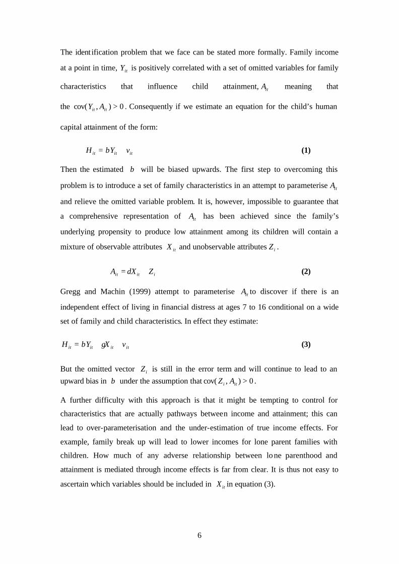
The ident ification problem that we face can be stated more formally. Family income
at a point in time, itY is positively correlated with a set of omitted variables for family
characteristics that influence child attainment, itA meaning that
the 0),cov( >itit AY . Consequently if we estimate an equation for the child’s human
capital attainment of the form:
ititit vYH += β (1)
Then the estimated β will be biased upwards. The first step to overcoming this
problem is to introduce a set of family characteristics in an attempt to parameterise itA
and relieve the omitted variable problem. It is, however, impossible to guarantee that
a comprehensive representation of itA has been achieved since the family’s
underlying propensity to produce low attainment among its children will contain a
mixture of observable attributes itX and unobservable attributes iZ .
iitit ZXA += δ (2) Gregg and Machin (1999) attempt to parameterise itA to discover if there is an
independent effect of living in financial distress at ages 7 to 16 conditional on a wide
set of family and child characteristics. In effect they estimate:
itititit vXYH ++= γβ (3)
But the omitted vector iZ is still in the error term and will continue to lead to an upward bias in β under the assumption that 0),cov( >iti AZ .
A further difficulty with this approach is that it might be tempting to control for
characteristics that are actually pathways between income and attainment; this can
lead to over-parameterisation and the under-estimation of true income effects. For
example, family break up will lead to lower incomes for lone parent families with
children. How much of any adverse relationship between lone parenthood and
attainment is mediated through income effects is far from clear. It is thus not easy to
ascertain which variables should be included in itX in equation (3).
7
Alternative Strategies and Previous Literature
Disentangling income effects from unobserved family or child heterogeneity requires
some ingenuity and a careful statement of econometric models. To our knowledge,
three approaches have been most widely used in the context of educational attainment
(Blow et al. 2004, provide a comprehensive literature review for this area). The
majority of these strategies exploit variations in incomes within families rather than
longer term income differences which may have larger effects.
i) Experimental Trials of Policy Interventions
In the US there have been a number of welfare to work programmes undertaken under
experimental conditions and evidence from these is perhaps the cleanest and clearest
available. The relevant population in the trial is divided into a treated group who
participate in the programme and an untreated control group. This random allocation
ensures that treatment is not correlated with family or child characteristics. Such
trials became more common from 1996 when the Clinton administration allowed
states to administer their own welfare to work programmes. Under these programmes
the treated receive an exogenously driven change in family income which is not
received by the untreated programme families. In all cases the financial payment is
attached to other conditions, but they can be nonetheless informative.
Some welfare reforms that focus on getting lone mothers into employment (and off
welfare) have included child outcomes in their evaluations. The most recent and
comprehensive assessment of the effects on children is contained in Clark-Kauffman
et al. (2003); we report the key results from this paper in Table 2.
This analysis pools the data from a large number of random assignment welfare
experiments and compares the treated and control groups. These programmes were
aiming to raise employment and earnings of welfare dependent families in the US;
some also offered additional cash assistance when mothers moved into work. Column
1 reports the evidence of programme effects on child educational attainment test
scores for those programmes with cash assistance, so that the observed changes in
child outcomes reflect the combined effect of work and income changes. The income
gains among the treated participants in these earning-supplement programmes where
modest at $1500-$2000 (£1000 to £1300) per year over the untreated participants for
8
two to three years. Column 2 shows the impact on child test scores for programmes
based on raising maternal employment without additional in-work financial support
(job search counselling or education based approaches). These had positive
employment and earnings effects but had very modest effects on family incomes, as
benefit payments are withdrawn. The differences between columns 1 and 2 reflect the
impact of the extra effect of income as both types of programmes led to similar
employment and earnings changes. The size of the attainment gains for pre-schoolers
is modest, but statistically significant, raising attainment by 8 percent of a standard
deviation. At older ages there are no differences across the programmes except that at
ages 12 to 15 there are large, but poorly identified, negative results associated with the
programmes without earnings supplement.
Another interesting set of experimental programmes are the evaluations of the Moving
To Opportunity (MTO) programme (see Goering and Feins, 2003 for a full summary).
In these programmes families from poor neighbourhoods are randomly selected into
one of three populations. The first is given financial help with rents conditional upon
moving to a more affluent neighbourhood. 4 A second group received rent support
but could move to any neighbourhood. The third group received no help in moving
from the deprived neighbourhood. So the treatment is that families receive financial
support to meet higher housing costs associated with moving to more affluent (and
high rent) areas, provided they make the move.
These studies provide crucial evidence of how higher incomes might influence
children’s educational attainment by enabling families move to live in affluent areas
with better schools and peer groups. Importantly these moves were not associated
with increases in employment or earnings among adults, so the effects observed are
operating purely through neighbourhood change. Table 3 reports details of child
outcomes across studies from two MTO sites in Boston and Baltimore, as reported in
Goering and Feins (2003). The results suggest that moving neighbourhood (which is
hand- in-hand with changing school and peer group for most children) is associated
with marked improvements in behavioural problems and school test scores and, for
older children, a reduction in the number of arrests for violent crime.
4 The rent assistance was in the form of Section 8 housing vouchers. This is a rent assistance programme in the US which has some parallels with Housing Benefit in the UK but is more restricted in its availability.
9
These studies provide powerful evidence for income effects on child outcomes,
however, the specific samples involved and the enforced link between income
increases and other changes (employment or moving neighbourhood) may mean the
results do not generalise to the population at large.
In the UK random-assignment experiments are very rare; however there is one policy
evaluation that is relevant to our context. The Education Maintenance Allowance was
piloted in 15 Local Authorities in the UK from 1999 onward. It offered youths from
low income families a weekly financial payment (of up to £40 a week), for up to two
years, provided they stayed on in full- time education after compulsory schooling ends
at age 16. Non-attendance leads to payment withdrawal and there were bonuses for
course completion. The EMA is therefore a means tested cash payment conditiona l on
educational enrolment. Ashworth et al. (2003) report evidence of the impact of this
programme where eligible and ineligible populations in the pilot areas are compared
(through propensity matching techniques) to similar people in 11 areas not taking part
in the programme. The evaluation suggests school/college enrolment increased by 6
percentage points for those eligible for full subsidy. Additionally there was no
increase in drop out rates and staying on rates into a second year also improved. The
EMA is being implemented nationally at the start of the 2004-2005 academic year.
ii) Sibling Studies
Our model of attainment and income is:
itititit vXYH ++= γβ . (4)
The principle behind sibling fixed effects models is to assume that the error itv is
composed of two elements itfit eZv += where fZ is a family fixed effect which is
equal across siblings and ite is uncorrelated with itY . The sibling fixed effects model is
estimated on deviations of itH and itY from the family mean; this eliminates the
impact of fZ and generates unbiased estimates ofβ .
The variation in family incomes experienced by the siblings comes from the age gap
between them. This means that siblings will be affected by income in different periods
10
because other children have either not been born yet or have already left home. This
approach uses income variations within a family rather than differences across
families. Sibling studies require an income history for the family including some
periods of differing income experience.
The central problems for sibling studies is that siblings will often be close in age and
experience very similar income patterns for most of their childhood. Also, only
families with two or more children can be considered. Further, measurement error in
data reporting will lead to attenuation bias. An advantage of this approach is that
income shocks in the family will be experienced by siblings at different ages; this can
provide evidence on when in childhood income matters most. Levy and Duncan
(2000) is a recent sibling study using the Panel Study of Income Dynamics. They find
that parental income matters most for young children but that the magnitudes of the
effects are small with a 2.7 fold increase in family income through childhood adding
three quarters of a year to completed years of schooling by age 20. These are
extremely small impacts compared with others found in the literature.
(iii) Post Educational Income
Mayer (1997) also considers whether transitory income fluctuations have an impact
on child educational outcomes. Leaving aside the question of measurement error,
income at a point in time can be thought of as composed of transitory and permanent
components.
transit
permiit YYY += (5)
Therefore in a regression of the relationship between income and education the
income parameter will be a weighted-average of the coefficients that would be
obtained if measures of permanent and transitory income could be entered into the
model separately. The key assumption here is that the permanent component will be
correlated with unobservable characteristics iZ and that this leads to bias. The
transient income component is assumed to be uncorrelated with fixed family
characteristics 0),cov( =itrans
i ZY , therefore the coefficient on transiY would be the true
relationship between income and education. The strategy is to use a measure of family
11
income after the child has completed the normal education process as a control for the
permanent component of income. The estimation equation thus looks like
itititit uYYH ++= +121 ββ (6)
Any correlation between the later income measure and attainment is not causal and its
inclusion can be seen as an attempt to condition out the permanent income
component. If 1+itY was perfectly correlated with permiY 1β would be the relationship
of interest between education and transitory income at age 16. However this will not
be the case as 1+itY also contains a transitory component, meaning some residual bias
will remain in this approach. This can be reduced by averaging over several years of
later income.
Mayer uses a range of child outcomes and test scores as dependent variables. The
addition of post-childhood family income reduces the estimated impact of a 10%
increase in income on years of schooling from 1.86 to 1.68 (after conditioning on
observed family fixed characteristics). The conditioning on later income makes only a
minor difference but is more important for other outcomes such as teenage
motherhood and dropping out of school. A concern with this approach is that income
changes between the two periods considered reflect family shocks that influence child
attainment independently. In addition, lifecycle models predict that anticipated
income changes will affect behaviour in all periods if families can smooth
consumption.
The US literature consistently shows that family income does influence a child’s
educational attainment. However, as studies consider a range of outcomes and
sometimes refer to specific population groups or ages of children, it is difficult to
form a clear picture of the results across identification strategies. The identified causal
income effects appear small in the sibling study but much larger in the work by Mayer
described above, and in the experimental studies. The majority of the identification
strategies focus on income variations that are unrelated to fixed family characteristics.
Naturally such variations tend to be small. They would not show the impact of
changes in income sufficient to change residential neighbourhood, for example, which
is so important in determining peer group and school quality. In this regard the MTO
12
experiments are particularly revealing; showing that neighbourhood makes a
substantial difference to child educational and behavioural outcomes.
British work on uncovering the causal impact of income on education is less well-
developed than the research on US data. As has already been mentioned Gregg and
Machin (1999) try to isolate the impact of financial disadvantage by carefully
controlling for confounding factors. Ermisch et al. (2002) use the sibling methods
described here on BHPS data to try and uncover the effect of parental employment
(rather than income) on educational attainment. In the following sections we explore
the extent to which the data available in the UK enables us to identify the impact of
income on educational attainment.
3. Data
The primary data sources used in this paper are the British Cohort Study (BCS) and
the British Household Panel Study (BHPS). These data have different strengths and
weaknesses but both offer the possibility of examining the relationship between
family income variations and the child’s educational outcomes.
The BCS takes all children born in the same week in April 1970 and follows them at
intervals until, to date, age 30. This data is particularly useful for our purposes as it
contains substantial information on family background and child characteristics
collected at ages 5, 10 and 16. Information on school leaving decisions and final
educational attainment s are available from the age 16 and 30 surveys.
The BCS contains two measures of family income, at ages 10 and 16. Having two
measures allows us more scope to control for permanent income differences. However
the income measures are not problem-free. In order to encourage response all
questions ask parents to identify the income band they fall into rather than attempting
to obtain a precise income measure. By considering similar families in the Family
Expenditure Survey we find the median income within each band and set incomes to
this value. Another important set of data we use is from tests administered to the
children at age 10. We use the quintile attained in the Shortened Edinburgh Reading
Test and Young’s friendly maths test. Measures of test scores and income at age 10
enable us to consider the relationship between the change in attainments between ages
13
10 and 16 and the change in incomes, removing the permanent effect of
characteristics correlated with income.
The first results we report below also include data from the National Child
Development Study (NCDS). This data was the forerunner to the BCS, considering
children born in a week in March 1958. The information available in the NCDS is
very similar to the BCS, however, income information is only obtained once, at age
16; this limits the extent to which this data can be used to identify the causal impact of
income.
The BHPS is a household panel study which started in 1991 with 10,000 households.
Households have been sampled annually since and the most recent data available is
from 2001. The advantage of this data is that we have annual measures of income for
all households and information on educational qualifications and enrolment for all
children and young people within the sample households. These aspects enable us to
pursue two identification strategies which are not possible using the BCS data. First,
parental household income continues to be observed after young people have left
home, enabling us to pursue Mayer’s idea that later incomes will not be directly
correlated with outcomes aside from their correlation with permanent income.
Second, the inclusion of all children enables us to use sibling variation to eliminate
family fixed effects as in Levy and Duncan (2001) and Ermisch and Francesconi
(2002).
The main disadvantage of the BHPS is its small effective sample size; there are few
children of a particular age in each wave. This is particularly limiting for those
estimations which require the observation of young people in several waves. We
attempt to maximise samples by using information from other waves whenever
possible. Nonetheless this limitation of the data sometimes affects the specifications
we can estimate. In addition the BHPS contains no information on test scores; the
attainment information available is age left full time education and educational
qualifications obtained.
4. Results
We begin this section by estimating some basic models of how income and
educational attainment are related in three time periods using data from the NCDS,
14
BCS and BHPS as described previously. We add controls for a series of family
characteristics in order to show the extent to which the patterns are modified by the
most straight- forward attempts to reduce the bias on the income effect. In the final
estimation we control for a group of variables for which it is less clear whether they
independently drive attainment or just mediate the relationship between income and
education. These provide the strictest test of this type of model.
The models estimated are ordered probits of the highest qualification obtained related
to family income at age 16. Highest qualification has four categories: degree or
equivalent; A levels or equivalent; GCSEs at A-C, CSEs at Grade 1, O levels or
equivalent; and below this level. This measure is obtained from the age 33 data in the
NCDS, the age 30 data in the BCS and at age 23 (or 22 if age 23 unavailable) in the
BHPS. There is an obvious non-comparability here as highest qualification is taken at
a much earlier age in the BHPS than in the other samples. This could potentially bias
the income effects in the BHPS upwards if poorer young people take longer to reach
their final qualification level, unfortunately this is unavoidable given the nature of the
BHPS data. Reassuringly, results presented in Blanden and Machin (2004) show
similar patterns for degree attainment when we consider graduation by age 23 in all
the datasets.
The first panel in Table 4 presents results showing the association between family
income and highest qualification with no controls added. In order to ease
interpretation marginal effects are calculated to show the change in probability of
obtaining the lowest and highest qualification category in response to an income
shock, we show the impact on probabilities of a constant one third reduction in
income (.4 log points). To give an idea of the magnitude of the shock; in these data a
reduction of 33% from the mean is equivalent to moving from the median to around
the 20th percentile.
The first key point is that the raw relationship between family income and education
has strengthened considerably between the NCDS and BCS cohorts. The marginal
effect of reducing income by .4 log points for the NCDS is to increase the chance of
obtaining less than a GCSE A-C equivalent by 8.1 percentage points and reduces the
probability of obtaining a degree by 4 percentage points. In the BCS a one third shock
15
increases the chance of poor qualifications by 9.6 percentage points and reduces the
probability of obtaining a degree by 7.4 points.
In the BHPS the implied marginal effect of obtaining no qualifications falls relative to
the BCS, back to 5.7 points, whilst the change in the probability of going on to do a
degree strengthens to 8.7 points. There is therefore prima facie evidence of an opening
up in opportunities at lower levels of qualifications at the same time as there was a
strengthening of the education and income relationship at the higher education level.
These findings are consistent with those reported in Blanden, Gregg and Machin
(2003) and Blanden and Machin (2004) who find a reversal in the inequality in
staying on after the compulsory leaving age between students from richer and poorer
families but no evidence of a similar fall in higher education inequalities.
This approach shows the impact of the changing influence of income on attainment
but not the added effect of the increasing income inequality that was demonstrated in
Figure 1. In our data the standard deviation of log income rises from .402 in the
NCDS, to .481 in the BCS and .522 in the BHPS. If we estimate marginal effects that
take into account the increase in inequality over the period (by estimating the impact
of a standard deviation shock) marginal effects rise from -4 points in the NCDS, to -
8.6 points in the BCS and -11.1 points in the BHPS for the probability of doing a
degree. These compare to marginal effects of -4, -7.4 and -8.7 for the constant .4
shock. This shows how increased inequality magnifies the impact of the changes in
the strength of the relationship between education and income; in this example
growing inequality increases the marginal effects by 1.2 percentage points in the BCS
and 2.4 points in the BHPS.
In the remainder of the panels in this Table we add controls for family background.
The second panel adds controls for the child’s sex, family size, parental age and race;
this makes no substantive difference to the estimated income relationships. The third
panel adds controls for parental education5. This is one of the main observable
characteristics that we might think is correlated with both child’s attainment and
parental income. The implied income relationships are reduced by around a fifth to a
5 To avoid complications in cases where the father may not be a member of the household we control for mother’s education except in cases where the mother is missing when we use father’s education instead.
16
quarter. So even with these controls included the income effects remain strong and the
patterns over time are unchanged. For example, in the top panel a fixed .4 log point
drop in income led to a 4 point fall in the probability of obtaining a degree in the
NCDS compared with 7.4 points in the BCS and 8.7 points in the BHPS. Controlling
for parental education these marginal effects are 2.8, 5.6 and 6.7 points respectively.
Once again we can also allow the results to reflect rising income equality by applying
a standard deviation shift in income, the increase is again magnified to 2.8 (NCDS),
6.5 (BCS) and 8.6 (BHPS).
The final panel in Table 4 conditions on a larger set of additional controls for which it
is less clear whether or not they should be included. As noted in the earlier discussion
we would wish to condition on factors that influence both income and child
attainment but not factors that have an impact on attainment that is mediated though
income. Including a control for living in a lone-parent household, for example, might
wrongly attribute an effect to lone parenthood whereas it is actually the low income
associated with lone parenthood that is the key issue. The factors introduced here are
region, social class and lone parenthood. Once again adding these controls leads to a
reduction in all the estimated relationships but here the interpretation is more
problematic.
Table 4 gives a clear picture of how the relationship between incomes at age 16 and
highest qualification has changed over time. However it would not be justifiable to
say we have uncovered changes in the causal relationships. In the next section we use
techniques borrowed from the US literature to explore the extent to which these
impacts are causal. Unfortunately the different strengths and weaknesses of the
datasets mean that no approach is applicable to the NCDS or to more than one of the
other datasets, even so, we believe the exercise is informative.
Income Variation and Child Attainment
The results presented above use income at age 16 as the variable of interest, this
includes permanent income through childhood, transient income at age 16 and any
measurement error.
161616 itrans
iperm
ii YYY ε++= (7)
17
As discussed earlier the main concern with estimating income effects is that the
permanent income component is correlated with fixed family characteristics that
influence attainment. All the strategies pursued below attempt to control for
permanent income effects and identify only the relationship between transient income
and education. This has three very important implications. First, the implied time over
which the income effect would have been applied to the family is much smaller.
Transitory income, by definition, only applies for a small number of years whereas
permanent income has an influence throughout childhood. Second, any measurement
error will become an increasingly important proportion of the variance of income
once the permanent income component is removed. This will bias our estimated
effects downward. Third, by focusing on transitory income, income effects that
require sustained differences to make an impact (e.g. moving to a better
neighbourhood) cannot be captured. For these reasons the estimated effects of income
on attainment will be lower than the effect of permanent income differences.
Child Development Trajectories – Controlling for Age 10 Ability and Income
Our first attempt to control for unobserved heterogeneity uses the BCS data on
income and ability tests at age 10 to control for differences between children up to this
age. This shows how income changes after age 10 influence educational attainment
after this age.
Assuming that the measures are good, controlling for ability scores at age 10 accounts
for the underlying differences in ability between children, one aspect of heterogeneity
which we believe will be correlated with income (our iZ ). However, it may still be
the case that unobserved heterogeneity impacts the achievement trajectory post-16 in
a way that is correlated with permanent income. In order to account for this we also
control for income at age 10. This will control for the part of income at age 16 which
is correlated with income at age 16, in other words the permanent component that may
be correlated with iZ .
Controlling for income and ability at age 10 is similar to adopting a model in which
the change in attainment after age 10 is regressed on the change in income between
age 10 and 16, meaning that we eliminate iZ in the style of a fixed effect model. As it
is likely that family background will affect development after age 10 as well as before
18
we also include a set of observable family characteristics; however to the extent that
there are aspects of family background correlated with income that are still
unobserved the coefficients will remain upward biased.
We control for income at age 10 in two different ways. First we include age 10
incomes as a RHS variable. So the estimating equation is:
itiiiiiadult vXYYHH ++++= 1610216110 γββα (8)
Here the estimated β on income at 16 is purged of any cross correlation with income
at 10, family characteristics and test scores at age 10. To the extent that age 10 income
does not provide a perfect measure of permanent income (because of its own
transitory component) this approach will remain upward biased.
The second approach is to use the change in income between ages 10 and 16 as a
direct measure of transitory income:
itiiiiiadult vXYYHH ++−+= 161016310 )( γβα (9)
where )()( 101016161016 itrans
iitrans
iii YYYY εε +−+=− . (10)
Note that in addition to netting out permanent income in this approach we introduce
more measurement error; also, the coefficient 3β on )( 1016 ii YY − will be reduced if
transitory income at age 10 has an impact on attainment after age 10. As a result we
view the strict first difference model as producing a coefficient that is downward
biased. In summary, the two approaches used will provide plausible upper and lower
bounds on the true effect.
Results for this methodology are given in Table 5. We estimate these specifications
with two dependent variables: highest qualification at age 30 and staying on beyond
the school leaving age. Again we report the marginal effects of the standard .40 log
point reduction in income. The first column reports results without conditioning on
age 10 income for comparison purposes, this is equivalent adding controls for test
scores to specification C in Table 4. The second and third columns provide upper and
lower bounds for the effect of age 16 income conditioning on age 10 income. The
19
upper panel gives the results for highest qualification achieved while the lower panel
looks at staying on at 16. In column 2 a one third reduction in income increases the
propensity to achieve no A-C GCSEs by just over 3 percentage points and has a
similar magnitude reduction in the propensity to get a degree. The strict first
difference in column 3, which represents a lower bound estimate, is around 1
percentage point for each of these attainment levels6. The lower panel finds similar
but opposite signed effects for staying on as those for low qualification attainment.
Sibling Fixed Effect Estimation
The results of the sibling models for the BHPS are given in Table 6. Child-specific
controls are included to account for any characteristics which change across children
and may be correlated with income changes and attainment. In our models we control
for the gender of the child, the number of children in the household and the work
status of both parents when income is observed. Due to the shortness of the panel we
do not observe family incomes and full education histories for all siblings so the
results for different qualification levels use slightly different samples of individuals.
The top panel of Table 6 shows results for a linear probability model of staying on
and income at age 16. We show the impact for this model of only focusing on a
sample of siblings (column 2) rather than including single child families (column 1),
which makes no difference here. In the third column we remove bias in the same way
as we did in Table 4 by adding controls for parental education; this reduces the
income effect somewhat to –3.5 points for a one third reduction in income. The final
column estimates the sibling fixed effect models. Even in this stringent test of
causality the coefficient and marginal effect do not fall very much further; with a
marginal effect of –3.1 percentage points. If we believe the sibling fixed effects
models has removed the upward bias, this indicates that the true effect is around one
quarter smaller than that obtained in a model with only basic controls and more than a
tenth smaller than a model when parental education is also added. The disadvantage
6 The first difference model imposes the restriction that 213 βββ −= where 3β is the coefficient on
the change in income and 1β and 2β are the coefficients on income at age 16 and income at age 10 when these are entered separately, statistical tests show that the data does not reject this restriction in any of our models.
20
of the fixed effect approach is that the fall in the signal to noise ratio leads to a rise in
the standard errors leaving the income coefficient significant at only the 10% level.
The lower panel uses degree attainment as the dependent variable. In this case the
explanatory variable used is income at age 18. This seems appropriate as this is the
age when university enrolment choices are made for most young people. In addition,
choosing a measure of income obtained closer to the outcome maximises the available
sample size. For this model the income effects change more between the full sample
and sibling sample7. The marginal effect of a one third drop in income on the
probability of degree attainment is –6.2 with basic controls, -5.1 with controls for
parental education and –3.3 in the sibling fixed effects model. These reductions
indicate a proportionately larger bias in these estimates compared with those for
staying on. Although the magnitude of the sibling fixed effects coefficient remains
quite large the standard errors are high for this model and the coefficient and marginal
effect do not approach significance.
In summary, BHPS models that include sibling fixed effects give rather smaller
estimates than those that include only controls for family characteristics and in neither
case considered here are the estimates statistically significant at conventional levels.
The recurring problem of sibling estimation is that by relying on differences in
income within families for identification enhances the effect of measurement error
and reduces the variance in income and outcomes that can be used to identify effects.
This difficulty is clearly observed here as the standard errors rise sharply when sibling
fixed effects are included. Note also, that by comparing siblings who are close in age
the length of time over which income can be having an effect is sharply reduced.
These estimates are, therefore, more like point in time impacts of income at 16 on
post-16 education decisions rather than reflecting more cumulative effects of long-run
income differences. Due to these problems, the results of the sibling models can be
considered as a lower bound on the true income effect.
Post childhood income as a proxy for permanent family characteristics
7 This may be because to be included here siblings need to be fairly close together in age as income and outcome variables are further apart in time. It seems plausible that income constraints on university attendance are more important for parents who are contemplating sending two or more children to university in quick succession.
21
Table 7 explores Mayer’s approach using data from the BHPS. We add post-school
income to our specification in an attempt to proxy permanent income. In choosing the
age at which post-childhood income is observed we balance two factors. First,
income must be taken at an age sufficiently removed from the educational process to
satisfy the assumption that it will not be correlated directly with educational
outcomes. However, sample size considerations also play a role; the further away the
income is from the outcome of interest the smaller the sample size will be. We show
results conditioning on just income at age 20 and on an average of income between 18
and 21 (if age 21 income is not observed, we average up to age 20). Ideally we would
wish to use income at later ages but sample sizes become prohibitively small if this is
attempted.
The first panel reports the results from a probit model of highest qualification
achieved. In both models the impact of controlling for age 20 incomes is limited while
average income from age 18-21 reduces the impact of income somewhat more as we
would expect. In the model with no additional controls for income the marginal effect
of a .4 log point reduction in income is a 4.4 percentage point rise in the probability of
obtaining GCSE A-C qualifications and a 6.9 fall in the probability of obtaining a
degree, these effects reduce to 3.9 and 6.1 respectively when average income between
18 and 21 is controlled for.
The lower panel uses staying on at 16 as the dependent variable and finds similar
results (with reverse sign) as for ga ining poor or low qualifications. The evidence
suggests that in the 1990s family income has a larger effect on the probability of
obtaining a degree than it does on staying on or obtaining at least some good
secondary qualifications. These relative magnitudes are very much consistent with the
results in Table 4 and those found in related work by Blanden, Gregg and Machin
(2003). In summary, this approach reduces the observed income effect rather less than
the methods that control for earlier ability and income and the sibling fixed effect
approach.
6. Conclusions
This paper presents evidence on two questions, first whether there is a causal impact
of family income on educational attainment, and second whether the association
22
between family income and attainment is increasing. Our evidence clearly indicates
that there exist some important relationships between family income and educational
attainment in the UK and that these relationships have been strengthening through
time. In addition, as far as the data allows, we have also found evidence that income
does have a causal impact on educational outcomes. Evidence on changes over time in
the causal relationship between income and attainment is inconclusive as it is
impossible to estimate any of our most stringent models in a consistent way across the
datasets.
Although not all of our estimates are statistically significant, the consensus from our
different approaches suggests that family income does affect educational outcomes.
The models which attempt to net out permanent income (and therefore provide a
lower bound estimate) suggest that a one third reduction in family income from the
mean, which is about £140 a week or £7000 a year, reduces the chances of securing a
degree by around 4 percentage points. The estimates based on only conditioning out
family characteristics are somewhat larger. Effects of a similar magnitude are found
for the other outcomes we consider, obtaining no GCSE A-C grades and staying on at
school.
A natural question to ask is whether this is a large impact or not, especially as £7000
sounds like a large shock compared with the 4 percentage point change it leads to. In
order to bring this into focus we can use our models to predict the difference between
the probability of degree attainment for young people at the 90th percentile of the
income distribution compared to the 10th percentile. The model which controls for
age 10 ability and income using BCS data predicts that the probability of degree
attainment is .18 at the 10th percentile compared with .27 at the 90th. Results from the
BHPS which control for post-education income give a larger estimate of the income
effect. This, combined with greater income inequality, means that the predicted gap is
larger with the probability of degree attainment at the 10th percentile .21 and .42 at the
90th. These results demonstrate that when combined with substantial income
inequality the impact of income has important implications for educational inequality.
From a policy point of view £7000 a year is a large amount of money, far beyond the
income redistribution that is likely to be achieved by taxes and benefits. However, a
broader attempt to reduce the inequalities in the distribution of work and wages offers
23
hope of more substantial progress. In addition, direct interventions to raise attainment
of those from poorer families, through early years’ education and extra resources for
schools can be cost effective if they are well targeted. Recent Government policy
seems to be making a concerted effort to address these issues with financial
redistribution to families and education investments ranging from pre-school
programmes through to the EMA. It is for future research to discover if these attempts
are successful in creating greater equality of opportunity.
24
References
Ashworth, K. Hardman, J. Woon-chia, L., Maguire, S, Middletin, S., Dearden, L. Emmerson, K. Frayne,C. Goodman, A. Ichimura, H. and Meghir, C. (2001) Education Maintainance Allowance: The First Year A Quattitive Evaluation, Department for Education and Employment Research Report no. 257
Atkinson, A. (1981) ‘On Intergenerational Income mobility in Britain’, Journal of Post-Keynesian Economics’, 3, 194-218.
Blanden, J., P. Gregg, A.Goodman and S.Machin (2002) ‘Changes in Intergenerationa l Mobility in Britain’, Centre for the Economics of Education Discussion Paper No.26, London School of Economics and forthcoming in M. Corak (ed.) Generational Income Mobility in North America and Europe, Cambridge University Press.
Blanden, J., P.Gregg, S. Machin (2003) ‘Changes in Educational Inequality’ Mimeo, Centre for Economic Performance.
Blanden, J. and S. Machin (2004) ‘Educational Inequality and the Expansion of UK Higher Education’, Scottish Journal of Political Economy, Forthcoming.
Blow, L., A. Goodman, G. Kaplan, I. Walker and F. Windmeijer (2004) ‘How Important is Income in Determining Children’s Outcomes? A Methodology Review of Econometric Approaches’ A Report for Her Majesty’s Treasury Evidence Based Policy Fund, Forthcoming as an IFS Discussion Paper.
Breen, R. and J. Goldthorpe (2001) ‘Class, Mobility and Merit: The Experience of Two British Birth Cohorts’, University of Oxford, Mimeo.
Brewer, M., A. Goodman, M. Myck, J. Shaw and A. Shephard (2004) ‘Poverty and Inequality in Britain: 2004’ Institute for Fiscal Studies Commentary No. 96.
Clark-Kauffman, E., G. Duncan and P. Morris (2003) ‘How Welfare Policies Affect Child and Adolescent Achievement’, American Economic Review, 93, 299-303.
Ermisch, J. M. Francesconi and D. Pevalin (2002) ‘Childhood Parental Behaviour Young Peoples Outcomes’ Institute for Social and Economic Research, Working Paper No 2002-12.
Feinstein, L. (2003) ‘Inequality in the Cognitive Development of British Data in the 1970 Cohort’, Economica, 70, 73-97.
Glennerster, H. (1995) British Social Policy since 1945, Blackwells, Oxford.
Gibbons, S. and S. Machin (2003) ‘Valuing English Primary Schools’ Journal of Urban Economics, 53, 197-219.
Goering, J. and J. Feins Eds. (2003) Choosing a Better Life? Evaluating the Moving to Opportunity Social Experiment, Urban Institute Press, Washington DC.
25
Gregg, P., S. Harkness and S. Machin (1999) ‘Poor Kids: Child Poverty in Britain, 1966-96’, Fiscal Studies, 20, 163-87
Gregg, P. and S. Machin (1999) ‘Childhood Disadvantage and Success or Failure in the Labour Market’, in D. Blanchflower and R. Freeman (eds.) Youth Employment and Joblessness in Advanced Countries, National Bureau of Economic Research, Cambridge, MA.
Gregg, P. and S. Machin (2000) ‘The Relationship Between Childhood Experiences, Subsequent Educational Attainment and Adult Labour Market Performance’, in Koen Vleminckx and Timothy Smeeding (eds.) Child Well Being in Modern Nations: What do we Know?, Policy Press.
Haverman R. and Wolfe, B. (1995) The Determinants of Children’s Attainments: A Review of Methods and Findings, Journal of Economic Literature, 23, 1829-1878
Hobcraft, J. (1998) ‘Intergenerational and life-course transmission of social exclusion: Influences and childhood poverty, family disruption and contact with the police’, CASE Paper 15, Centre for Analysis of Social Exclusion, LSE.
Houston, A. Granger, R. Bos, J. Mistry, R. Crosby, D. Duncan, G. McLoyd,V. Gibson, C. Magnuson, K Romich, J. Ventura, A. (2001) Work-based Anti-poverty Programs for Parents Can Enhance the School Performance and Social Behaviour of Children, mimeo Dept. of Human Ecology, University of Texas at Austin
Katz L.F., J.R. Kling and J. B. Liebman (2001) ‘Moving to Opportunity in Boston: Early Results of a Randomised Experiment’ Quarterly Journal of Economics 116, 607-654.
Levy, D. and Duncan, G. (2001) Using Siblings to Assess the Effect of Childhood Family Income on Completed Schooling, Joint Centre for Poverty Research Working Paper, North Western University.
Ludwig, J., G. Duncan and P. Hirschfield (2001) ‘Urban Poverty and Juvenile Crime: Evidence from a Randomised Housing Mobility Experiment’ Quarterly Journal of Economics, 116, 655-680.
Ludwig, J., H. Lad and G. Duncan (2001) ‘Urban Poverty and Educational Outcomes’ Brookings-Wharton Papers on Urban Affairs, 147-2001.
Mayer, S. (1997) What Money Can’t Buy: Family Income and Children’s Life Chances, Harvard University Press.
McGroeder, S. M. Zaslow, K. Moore and S. LeMenestral (2000) ‘The national evaluation of welfare to work strategies: Impacts on young children and their families two years after enrolment: Findings from the child outcomes study.’ Washington, DC. US Department of Health and Human Services.
Rowntree, B. S. (1901) Poverty, A Study of Town Life (London, Longman)
26
Figure 1: Changes Over Time in the Distribution of Real Income For Families With Children, UK
Table 1: Summary of Marginal Effects of Family Income at Age 16 on Educational Attainment
BCS – 1970 Birth Cohort
(1) (2) (3) (4) (5) From Table 4 From Table 4 From Table 5 From Table 5 Controlling for
parental education and basic controls
(1) Plus Controls for Social Class, Region and Lone-Parenthood
(1) Plus Controlling for age 10 income and ability at age
10
Change in income between ages 10 and 16
as the explanatory variable, controls as (3)
Range of Estimates
No A-C GCSEs or equiv.
.071 (.005)
.062 (.005)
.034 (.007)
.011 (.005)
.011 to .071
Staying on -.039 (.009)
-.009 (.008)
-.039 to -.009
Degree Attainment
-.056 (.003)
-.049 (.004)
-.029 (.005)
-.010 (.005)
-.010 to -.056
BHPS – Sample born 1974-1979 (5) (6) (7) (8) (9) From Table 4 From Table 4 From Table 6 From Table 7 Controlling for
parental education and basic controls
(5) Plus Controls for Social Class, Region and Lone-Parenthood
Sibling Fixed Effects Model
Controlling for average post-school income, plus
controls from (5)
Range of Estimates
No A-C GCSEs or equiv.
.043 (.008)
.022 (.008)
.039 (.008)
.022 to .043
Staying on -.031 (.020)
-.039 (.016)
-.031 to -.039
Degree Attainment
-.067 (.010)
-.038 (.012)
-.033 (.063)
-.053 (.013)
-.033 to -.067
Notes
1. The O level was the GCSE A -C equivalent when the BCS cohort left school, however some may have obtained GCSEs in more recent years.
2. Marginal effects are calculated as the average impact of a .4 reduction in log income, which is approximately a third reduction in the level of income.
3. The results shown in this table can be found in later in the paper in the tables stated, where they are highlighted in bold. More details about the estimates can be found in the notes and text that accompany these tables.
4. All models control additionally for ‘basic controls’ which are the child’s sex, ethnicity and dummies for number of siblings in the household and for parent’s age group.
28
Table 2: The Impact on Test Scores of Welfare to Work, Results from Experimental Evaluations
Treatment Effects on Test Scores (1) (2)
Treatment Age
Earnings-Supplement Programmes
All Other Programmes
Age 0-2 0.082** (0.034)
-0.016 (0.074)
Age 3-5 0.080** (0.026)
0.035 (0.026)
Age 6-8 -0.025 (0.033)
-0.015 (0.070)
Age 9-11 -0.043 (0.040)
-0.046 (0.082)
Age 12-15 -0.039 (0.060)
-0.167 (0.102)
R-squared .0346
.0409
Observations 18641
11982
Notes:
1. Source: Clark-Kauffman et al. (2003), Table 1. 2. The dependent variable is a within -study standardised measure of attainment, the precise
nature of this varies by the study and in some cases more than one measure is provided. 3. Controls are included in all models for follow-up length, prior earnings, prior earnings
squared, prior AFDC receipt, prior years of employment, high school degree, teen parent, marital status, number of children and age of youngest child.
4. Dummies are also added for the type of achievement measure and the study that the data is taken from.
5. * Statistically significant at the 10-percent level. 6. ** Statistically significant at the 5-percent level.
29
Table 3: Impacts of the Moving to Opportunity Programme
Mean outcomes by sample group (1) (2) (3)
Type of Impact Population MTO Treatment
group
Section 8 comparison
Control group
Differences in Child Behaviour
Children aged 6 to 15
Behavioural Problems – boys
23.6** 21.3** 32.6
Behavioural problems – girls
17.0 14.3 19.3
Number of Arrests for violent crimes per 100 juveniles
Children aged 11 to 16
1.4** 1.6* 3.0
Differences in School Tests Children aged 5 to 12
Elementary School CTBS percentile reading scores
32.47** 31.52** 25.13
Elementary School CTBS percentile math scores
36.25** 30.25 28.77
Note: 1. Differences in child behaviour come from the Boston study of Katz, Kling and Leibman
(2001), Table 6. 2. Violent crime results are from Baltimore study of Ludwig, Duncan and Hirschfield (2001)
which are summarised in Table 6.3 of Goering and Liebman (2003) 3. The test scores results are from the Baltimore study of Ludwig, Ladd and Duncan (2001) and
are summarised in Table 6.1 of Goering and Liebman (2003). 4. Behavioural problems are measured as the fraction of the seven types of behaviour that the
child shows. For example, if he shows one type this score will be .142 (1/7) 5. CBTS is the Comprehensive Test of Basic Skills. 6. ** indicates that the treated group mean differs from the control group mean at a 5-percent
level * shows that this difference is significant at the 10-percent level.
30
Table 4: Relationship between Highest Qualification and Income at Age 16
Marginal Effects of Log Income at Age 16 from Ordered Probit Models (1) (2) (3)
A. No Controls
NCDS 1958 BCS 1970 BHPS 1975-80
No A-C GCSEs .081 (.005)
.096 (.004)
.057 (.008)
Degree Attainment -.040 (.002)
-.074 (.003)
-.087 (.009)
(4) (5) (6) B. Specification A Plus Basic
Controls NCDS 1958 BCS 1970 BHPS 1975-80
No A-C GCSEs .082 (.006)
.095 (.004)
.054 (.008)
Degree Attainment -.040 (.002)
-.073 (.003)
-.082 (.009)
(7) (8) (9) C. Specification B Plus Parent’s
Education NCDS 1958 BCS 1970 BHPS 1975-80
No A-C GCSEs .057 (.005)
.071 (.005)
.043 (.008)
Degree Attainment -.028 (.002)
-.056 (.003)
-.067 (.010)
(10) (11) (12) D. Specification C Plus Region, Social Class and Lone Parent
Status
NCDS 1958 BCS 1970 BHPS 1975-80
No A-C GCSEs .039 (.005)
.062 (.005)
.022 (.008)
Degree Attainment -.020 (.003)
-.049 (.004)
-.038 (.012)
Sample size 7138 4708 580 Notes:
1. The dependent variable is highest qualification which is coded as 1 “No qualifications, or qualifications below GCSE A-C or equivalent” 2 “GCSE A-C or equivalent” 3 “A level of equivalent” 4 “Degree or equivalent”. For the NCDS this variable is measured at age 33, for the BCS at age 30 and for the BCS age 23 (or 22 if this is not available).
2. All family income data is in 2001 prices. 3. In all the BHPS specifications controls are added for year of birth and the wave in which the
child is 16. 4. Basic controls are the child’s sex, ethnicity, dummies for number of siblings in the household
and controls for parents’ age group. 5. Marginal effects are calculated as the average impact of a .4 reduction in log income, which is
approximately a third reduction in the level of income. This is £98 at the mean for the NCDS, £96 at the mean for the BCS and £140 at the mean for the BHPS.
6. Standard errors are in parenthesis, these are obtained from a bootstrap procedure for marginal effects.
31
Table 5: Relationship between Educational Attainment and Income at 16: Controlling for Earlier Income and Test Scores in the BCS
Ordered Probit Models of Highest Qualification
(1) (2) (3) Log Income at age
16 Log Income at age 16 with Log Income at
10 controlled
Change in Log Income Between 16
and 10 Coefficient
.420 (.044)
.312 (.050)
.098 (.046)
Coefficient on Age 10 Income
.240 (.057)
Marginal Effect on No A-C GCSEs
.046 (.006)
.034 (.007)
.011 (.006)
Marginal Effect on Degree Attainment
-.039 (.004)
-.029 (.005)
-.010 (.005)
Test score controls YES YES YES
Probit Models of Staying On (4) (5) (6) Log Income at age
16 Log Income at age 16
with income at 10 controlled
Change in Log Income Between 16
and 10 Coefficient
.438 (.053)
.299 (.062)
.065 (.056)
Coefficient on Age 10 Income
.307 (.070)
Marginal Effect on Staying On
-.056 (.007)
-.039 (.008)
-.009 (.008)
Test score controls YES YES YES
Notes: 1. All models include basic controls, maths and reading score quintile and parent’s education. 2. Marginal effects are calculated as the average impact of a .4 reduction in log income, which is
approximately a one third reduction in the level of income.
32
Table 6: Relationship between Educational Attainment and Income at 16: Controlling for Sibling Fixed Effects, BHPS
Linear Probability Model of Staying On in Post-Compulsory Education
(1) (2) (3) (4) No Fixed Effects
– Full Sample No Fixed Effects - Sibling Sample
(2) Plus Controls for Parent’s Education
Sibling Fixed Effects
Marginal Effect on Staying On
-.040 (.010)
-.042 (.012)
-.035 (.012)
-.031 (.020)
Sample Size 1613 984 984 984
Linear Probability Model of Obtaining a Degree by Age 23/22 on Family Income at age 18 (5) (6) (7) (8) No Fixed Effects
– Full Sample No Fixed Effects - Sibling Sample
(6) Plus Controls for Parent’s Education
Sibling Fixed Effects
Marginal Effect on Degree Attainment
-.034 (.012)
-.062 (.021)
-.051 (.020)
-.033 (.063)
Sample Size 709 309 309 309 Notes
1. Basic controls are once again added to these models as these are child specific at age 16. 2. Addition controls are added for parents work status in the year that income is observed as this
may be correlated with differential income and performance between siblings. 3. The definition of a sibling is an individual in the sample who shares the same parental
identifier. This is defined as the mother and father’s combined identifiers when both these are listed or the lone parent’s identifier where only one is listed. A wider sibling sample can be generated by matching just one parent; however this raises complications about how long children have been co-resident.
4. Marginal effects are calculated as the average impact of a .4 reduction in log income, which is approximately a third reduction in the level of income.
33
Table 7: Relationship between Educational Attainment and Income at 16: Controlling for Permanent Income Proxied by Later Income, BHPS
Ordered Probit Model of Highest Qualification by Age 23/22
(1) (2) (3) Log Income at age 16 Log Income at age 16
with Log Income at 20 controlled
Log Income at 16 with average of 18-21
income controlled Marginal Effect on No A-C GCSEs
.044 (.007) .041 (.007) .039 (.008)
Marginal Effect on Degree Attainment
-.069 (.009) -.065 (.011) -.061 (.012)
Sample Size 540 540 540 Probit Model of Staying On
(4) (5) (6) Log Income at age 16 Log Income at age 16
with Log Income at 20 controlled
Log Income at 16 with average of 18-21
income controlled Marginal Effect on Staying On
-.050 (.013) -.047 (.014) -.039 (.016)
Sample Size 856 856 856 Notes:
1. All models include basic controls and parent’s education. 2. Marginal effects are calculated as the average impact of a .4 reduction in log income, which is
approximately a third reduction in the level of income.