54
Fast algorithms for PDE and integral equations 18.336J/6.335J Class notes Laurent Demanet Draft April 23, 2014
Fast algorithms forPDE and integral equations
18.336J/6.335JClass notes
Laurent DemanetDraft April 23, 2014

2
Contents
1 Model problems 51.1 The Laplace, Poisson, and Helmholtz equations . . . . . . . . 51.2 Volume integral equations . . . . . . . . . . . . . . . . . . . . 51.3 Boundary integral equations . . . . . . . . . . . . . . . . . . . 51.4 Exercises . . . . . . . . . . . . . . . . . . . . . . . . . . . . . . 11
2 Fourier-based methods 132.1 PDE and discrete sine/cosine transforms . . . . . . . . . . . . 132.2 Integral equations, convolutions . . . . . . . . . . . . . . . . . 132.3 Krylov subspace methods . . . . . . . . . . . . . . . . . . . . 172.4 Ewald summation . . . . . . . . . . . . . . . . . . . . . . . . . 172.5 Nonuniform Fourier methods . . . . . . . . . . . . . . . . . . . 172.6 Exercises . . . . . . . . . . . . . . . . . . . . . . . . . . . . . . 17
3 Fast multipole methods 193.1 Projection and interpolation . . . . . . . . . . . . . . . . . . . 19
3.1.1 Polynomial interpolation . . . . . . . . . . . . . . . . . 223.1.2 Collocation . . . . . . . . . . . . . . . . . . . . . . . . 23
3.2 Multipole expansions . . . . . . . . . . . . . . . . . . . . . . . 243.3 The fast multipole method . . . . . . . . . . . . . . . . . . . . 28
3.3.1 Setup . . . . . . . . . . . . . . . . . . . . . . . . . . . 283.3.2 Basic architecture . . . . . . . . . . . . . . . . . . . . . 303.3.3 Algorithm and complexity . . . . . . . . . . . . . . . . 31
3.4 Exercises . . . . . . . . . . . . . . . . . . . . . . . . . . . . . . 34
4 Hierarchical matrices 374.1 Low-rank decompositions . . . . . . . . . . . . . . . . . . . . . 374.2 Calculus of hierarchical matrices . . . . . . . . . . . . . . . . . 41
3
4 CONTENTS
4.3 Hierarchical matrices meet the FMM . . . . . . . . . . . . . . 41
5 Butterfly algorithms 435.1 Separation in the high-frequency regime . . . . . . . . . . . . 435.2 Architecture of the butterfly algorithm . . . . . . . . . . . . . 43
A The Fast Fourier transform (FFT) 47
B Linear and cyclic convolutions 49B.1 Cyclic convolution . . . . . . . . . . . . . . . . . . . . . . . . 49B.2 Linear convolution . . . . . . . . . . . . . . . . . . . . . . . . 50B.3 Partial linear convolution . . . . . . . . . . . . . . . . . . . . . 51B.4 Partial, symmetric linear convolution . . . . . . . . . . . . . . 53
Chapter 1
Model problems
1.1 The Laplace, Poisson, and Helmholtz equa-
tions
1.2 Volume integral equations
1.3 Boundary integral equations
The idea of boundary integral equations is to reduce a PDE in some domainto an integral eqation on the surface of the domain, by means of the free-spaceGreen’s function. Let us first consider the Laplace equation in d dimensions(x = (x1, . . . , xd)). Let Ω be a bounded domain in Rd. Four problems are ofinterest:
• Interior problems.∆u(x) = 0, x ∈ Ω,
with either Dirichlet boundary conditions (u = f on ∂Ω) or Neumannboundary conditions (∂u/∂n = g on ∂Ω).
• Exterior problems.∆u(x) = 0, x ∈ Ωc,
with either Dirichlet boundary conditions (u = f on ∂Ω) or Neumannboundary conditions (∂u/∂n = g on ∂Ω), and a decay conditions atinfinity, namely
|u(x)| = O(|x|2−d).
5
6 CHAPTER 1. MODEL PROBLEMS
The interior Neumann problem is only solvable when g obeys the zero-mean admissibility condition (the topic of an exercise in section 1.4)∫
∂Ω
g(x)dSx = 0.
Let us focus on the special case of the exterior Dirichlet problem. If Ω is asphere of radius R in R3, and f = 1, then a multiple of the Green’s functionprovides the solution everywhere outside Ω:
u(x) = q1
4π|x|.
Matching with u(x) = 1 when |x| = 1 yields q = 4πR. The field u(x) solvesthe Laplace equation by construction, since the Green’s function is evaluatedaway from its singularity (here, the origin.) More generally, we can alsobuild solutions to the exterior Laplace problem as a superposition of chargesqj located at points yj inside Ω, as
u(x) =∑j
G(x,yj)qj.
With enough judiciously chosen points yj, the boundary condition u(x) =g(x) on ∂Ω can often be matched to good accuracy. The fit of the qj can bedone by solving u(xi) =
∑j G(xi,yj)qj for an adequate collection of xi on
∂Ω. Conversely, if the solution is sought inside Ω, then the charges can belocated at yj outside Ω.
This type of representation is called a desingularized method, becausethe charges do not lie on the surface ∂Ω. Very little is known about itsconvergence properties.
A more robust and well-understood way to realize an exterior solution ofthe Laplace equation is to write it in terms of a monopole density φ on thesurface ∂Ω:
u(x) =
∫G(x,y)φ(y)dSy, x ∈ Ωc, (1.1)
called a single-layer potential, and then match the Dirichlet boundary con-dition by taking the limit of x approaching ∂Ω. The density φ(y) can besolved from
f(x) =
∫G(x,y)φ(y)dSy, x ∈ ∂Ω. (1.2)
1.3. BOUNDARY INTEGRAL EQUATIONS 7
This latter equation is known as a first-kind Fredholm integral equation.Once φ is known, (1.1) can be used to predict the potential everywhere inthe exterior of Ω.
Notice that G(x,y) = log(|x − y|) is integrable regardless of the dimen-sion. The kernel G(x,y) = 1/|x−y| in 3D is also integrable when integratedon a smooth 2D surface passing through the point y, since in local polarcoordinates the Jacobian factor r cancels the 1/r from the integrand. Aslong as φ itself is bounded, there is no problem in defining the single-layerpotential as a Lebesgue integral. The same is true for the high-frequencycounterparts of the Poisson kernels. All these kernels belong in the class ofweakly singular kernels.
Definition 1. A kernel G(x,y) is called weakly singular in dimension n (thedimension of the surface over which the integral is taken, not the ambientspace) if it can be written in the form
G(x,y) = A(x,y)|x− y|−α,
for some 0 ≤ α < n, and A bounded.
The fact that G is weakly singular in many situations of interest has twoimportant consequences:
• First, when the density φ is bounded, it can be shown that u(x) definedby (1.1) is continuous for all x ∈ Ω. This fact is needed to justify thelimit x→ ∂Ω to obtain the boundary integral equation (1.2).
• Second, the operator TG mapping φ to f = TGφ in (1.2) is bounded onall Lp spaces for 1 ≤ p ≤ ∞, and is moreover compact (i.e., it is thenorm limit of finite rank operators).
Compactness, in particular, imposes a strong condition on the spectrumof TG. The eigenvalues must cluster at the origin, and nowhere else. Thisbehavior is problematic since it gives rise to ill-conditioning of discretizationsof TG, hence ill-posedness of the problem of solving for φ from f . This ill-conditioning is a generic, unfortunate feature of first-kind boundary integralequations.
An interesting alternative is to write the potential in Ωc from a dipolerepresentation on ∂Ω, as
u(x) =
∫∂G
∂ny
(x,y)ψ(y)dSy, x ∈ Ωc, (1.3)
8 CHAPTER 1. MODEL PROBLEMS
called a double-layer potential. The function ψ(x) can now be thought ofas a dipole density, since ∂G
∂nyis the potential resulting from a normalized
difference of infinitesimally close point charges. Again, we wish to match theDirichlet data f(x) by letting x → ∂Ω from the exterior, but this time thelimit is trickier. Because of the extra ∂/∂ny derivative, the kernel ∂G
∂ny(x,y)
is singular rather than weakly singular, and the double layer (1.3) is notcontinuous as x crosses the boundary ∂Ω (though it is everywhere else.)
For instance, in two and three space dimensions (hence n = 1, 2 for lineand surface integrals respectively), we compute
G(x,y) = log(|x− y|) ⇒ ∂G
∂ny
= −(x− y) · ny
|x− y|2,
and
G(x,y) =1
|x− y|⇒ ∂G
∂ny
= −(x− y) · ny
|x− y|3.
In order to precisely describe the discontinuity of (1.3) in x, let
K(x,y) =∂G
∂ny
(x,y), x,y ∈ ∂Ω.
Note that we reserve the notation K(x,y) only for x ∈ ∂Ω. Treating thecase x ∈ ∂Ω on its own is important, because gains extra regularity in thatcase. Consider the numerator (x− y) · ny in either expression above: whenx ∈ ∂Ω, we have orthogonality of the two vectors in the limit x→ y, yielding
|(x− y) · ny| ≤ c|x− y|2,
where the constant c depends on curvature. This implies that K(x,y) for x ∈∂Ω is less singular by a whole power of |x−y| than ∂G
∂ny(x,y) would otherwise
be outside of ∂Ω. From the expressions above, we now see that K(x,y) isbounded in two dimensions, and weakly singular in three dimensions. As aconsequence, the operator TK defined by
(TKψ)(x) =
∫K(x,y)ψ(y)dSy, x ∈ ∂Ω, (1.4)
is compact like TG was.The jump conditions for the double-layer potential (1.3) can now be for-
mulated. For x ∈ ∂Ω, let u−(x) be the limit of u(x) for x approaching ∂Ω
1.3. BOUNDARY INTEGRAL EQUATIONS 9
form the inside, and let u+(x) be the limit of u(x) for x approaching ∂Ω formthe outside. It is possible to show that
u−(x) =1
2ψ(x) + (TKψ)(x),
and
u+(x) = −1
2ψ(x) + (TKψ)(x).
The total jump across the interface is u+(x)− u−(x) = ψ(x).The boundary match is now clear for the double-layer potential in the
Dirichlet case. The boundary integral is either f(x) = 12ψ(x) + (TKψ)(x) in
the interior case, and f(x) = −12ψ(x) + (TKψ)(x) in the exterior case. Both
equations are called second-kind Fredholm integral equation.Since TK is compact, neither −I/2 + TK nor I/2 + TK can be (because
the identity isn’t compact). The respective accumulations points for theeigenvalues are at −1/2 and 1/2. This situation is much more favorablefrom a numerical point of view: second-kind integrals are in general wellconditioned, and Krylov subspace methods need relatively few iterations toconverge. The number of eigenvalues close to zero stays small, and the con-dition number does not grow as the discretization gets refined. For the twoDirichlet problems, the second kind formulation is therefore much preferred.
Both the single-layer potential and the double-layer potential formula-tions are available for the Neumann problems as well. Matching the normalderivative is trickier. For all x /∈ ∂Ω, we have
∂u
∂nx
(x) =
∫∂G
∂nx
(x,y)ψ(y)dSy. (1.5)
The kernel ∂G∂nx
(x,y) is the adjoint of the double layer potential’s ∂G∂ny
(x,y).
For x ∈ ∂Ω, equation (1.5) becomes the application of the adjoint of TK ,namely
(T ∗Kψ)(x) =
∫K(y, x)ψ(y)dSy, x ∈ ∂Ω.
The (1.5) is discontinous as x crosses ∂Ω, and inherits its jump conditionsfrom those of (1.3). Notice that the signs are reversed:
∂u
∂n−(x) = −1
2ψ(x) + (T ∗Kψ)(x),
10 CHAPTER 1. MODEL PROBLEMS
and∂u
∂n+
(x) =1
2ψ(x) + (T ∗Kψ)(x).
The single-layer potential therefore gives rise to a favorable second-kind in-tegral equation in the Neumann case – it is the method of choice. In theNeumann case the double-layer potential gives rise to an unwieldy hypersin-gular kernel that we will not deal with in these notes1.
There exist three prevalent discretization methods for boundary integralequations of the form u(x) =
∫K(x,y)φ(y)dSy.
1. Nystrom methods. Direct, though perhaps sophisticated quadrature ofthe kernel, and pointwise evaluation as
u(xi) '∑j 6=i
K(xi,yj)φ(yj)ωj,
for some weights ωj. Then solve for φ(yj).
2. Collocation methods. Expand φ(y) =∑
j φjvj(y) in some basis setvj(y), and evaluate pointwise to get
u(xi) '∑j
φj
∫K(xi,y)vj(y)dSy.
Then solve for φj.
3. Galerkin methods. Pick a basis set vj(x), expand φ(y) =∑
j φjvj(y),u(x) =
∑j ujvj(x), and test against vi(x) to get
∑j
ui〈vi, vj〉 =∑j
φj〈vi, TKvj〉.
Then solve for φj.
1Hypersingular kernels grow faster than 1/|x|n in n dimensions, but are well-defined inthe sense of distributions thanks to cancellation conditions. They are sometimes handlednumerically by the so-called Maue identities.
1.4. EXERCISES 11
1.4 Exercises
1. Show that the right-hand side g for the interior Neumann Laplace equa-tion must obey ∫
∂Ω
g(x)dSx = 0.
[Hint: use a Green’s identity.]

12 CHAPTER 1. MODEL PROBLEMS
Chapter 2
Fourier-based methods
2.1 PDE and discrete sine/cosine transforms
(...)
Throughout these notes we use the convention
Fjk = e−2πijk/N , (F−1)jk =1
Ne2πijk/N ,
with 0 ≤ j, k ≤ N − 1. Notice that F−1 = 1NF ∗.
2.2 Integral equations, convolutions
We consider the problem of computing potentials from charges. After dis-cretization, we have
uj =∑
Gjkqk,
where G is a Green’s function such as 12π
log(|x− y|) in 2D, or 14π|x−y| in 3D,
or even a Helmholtz Green’s function. The numerical values Gjk either followfrom a Galerkin formulation (finite elements), or a quadrature of the integral(Nystrom). The simplest Galerkin discretization of G consists in clusteringcharges inside panels.
Direct summation takes O(N2) operations. In this section we presentO(N logN) FFT-based algorithms for the summation u = Gq.
13
14 CHAPTER 2. FOURIER-BASED METHODS
• Periodic ring of charges. By translation-invariance, periodicity, andsymmetry, we get
u0
u1...
uN−1
=
g0 g1 . . . gN−1
g1 g0 . . . gN−2...
.... . .
...gN−1 gN−2 . . . g0
q0
q1...
qN−1
(2.1)
with gj = gN−j. In other words, Gjk = gj−k. The resulting matrix isboth Toeplitz (constant along diagonals) and circulant (generated bycyclic shifts of the first column). It is the circulation property whichenables a fast Fourier-based algorithm. The expression of u can alsobe written as a cyclic convolution:
uj = (g ? q)j =N−1∑k=0
g(j−k) modN qk,
where mod is the remainder of the integer division by N .
The discrete Fourier transform diagonalizes cyclic convolutions: it is agood exercise to show that
(F (g ? q))k = (Fg)k(Fq)k,
or, in matrix form,
g ? q = F−1ΛFq, Λ = diag(F (g)).
The fast algorithm is clear: 1) Fourier-transform q, 2) multiply compo-nentwise by the Fourier transform of g, and 3) inverse Fourier-transformthe result. Notice that we also get fast inversion, since q = F−1Λ−1Fu.
• Straight rod of charges. The formulation is the same as previously,namely (2.1) or Gjk = gj−k, but without the circulant property gN−j =gj. We are now in presence of a Toeplitz matrix that realizes an “ordi-nary” convolution, without the mod operation:
uj =N−1∑k=0
gj−kqk,
2.2. INTEGRAL EQUATIONS, CONVOLUTIONS 15
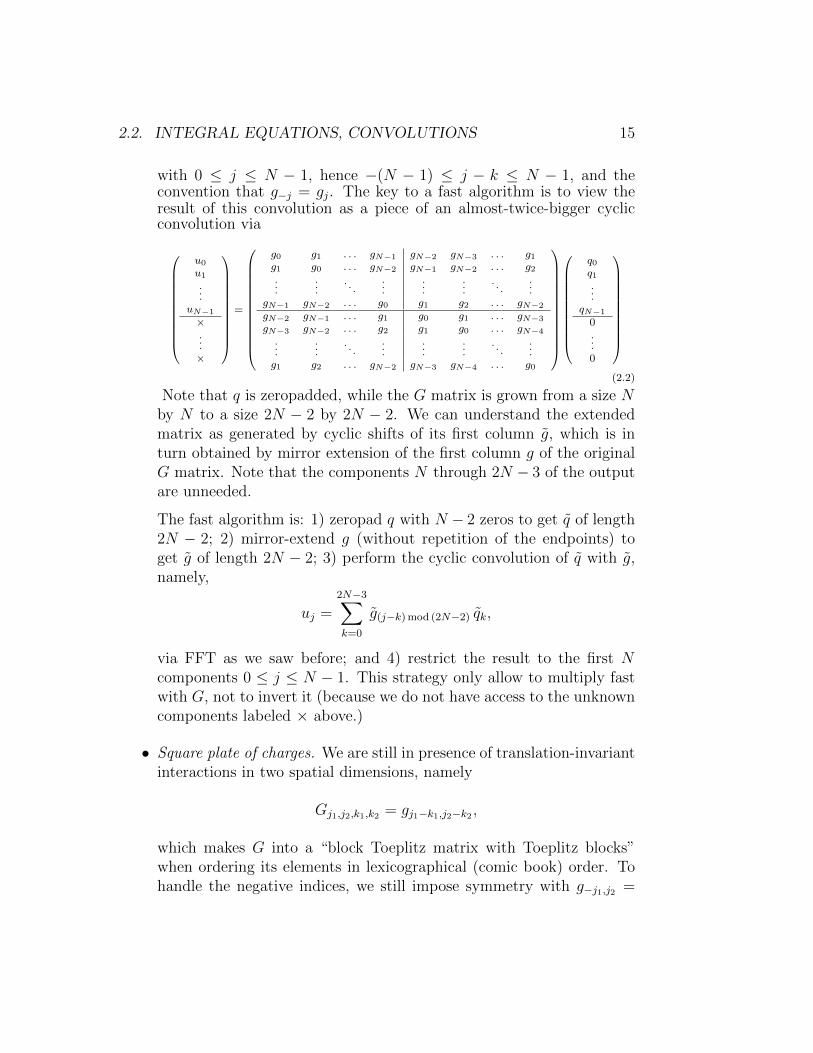
with 0 ≤ j ≤ N − 1, hence −(N − 1) ≤ j − k ≤ N − 1, and theconvention that g−j = gj. The key to a fast algorithm is to view theresult of this convolution as a piece of an almost-twice-bigger cyclicconvolution via
u0u1...
uN−1
×...×
=
g0 g1 . . . gN−1 gN−2 gN−3 . . . g1g1 g0 . . . gN−2 gN−1 gN−2 . . . g2...
.... . .
......
.... . .
...gN−1 gN−2 . . . g0 g1 g2 . . . gN−2
gN−2 gN−1 . . . g1 g0 g1 . . . gN−3
gN−3 gN−2 . . . g2 g1 g0 . . . gN−4
..
....
. . ....
......
. . ....
g1 g2 . . . gN−2 gN−3 gN−4 . . . g0
q0q1...
qN−1
0...0
(2.2)
Note that q is zeropadded, while the G matrix is grown from a size Nby N to a size 2N − 2 by 2N − 2. We can understand the extendedmatrix as generated by cyclic shifts of its first column g, which is inturn obtained by mirror extension of the first column g of the originalG matrix. Note that the components N through 2N − 3 of the outputare unneeded.
The fast algorithm is: 1) zeropad q with N − 2 zeros to get q of length2N − 2; 2) mirror-extend g (without repetition of the endpoints) toget g of length 2N − 2; 3) perform the cyclic convolution of q with g,namely,
uj =2N−3∑k=0
g(j−k) mod (2N−2) qk,
via FFT as we saw before; and 4) restrict the result to the first Ncomponents 0 ≤ j ≤ N − 1. This strategy only allow to multiply fastwith G, not to invert it (because we do not have access to the unknowncomponents labeled × above.)
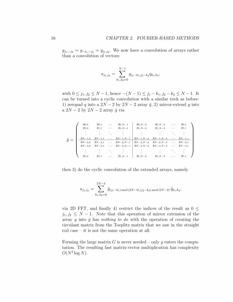
• Square plate of charges. We are still in presence of translation-invariantinteractions in two spatial dimensions, namely
Gj1,j2,k1,k2 = gj1−k1,j2−k2 ,
which makes G into a “block Toeplitz matrix with Toeplitz blocks”when ordering its elements in lexicographical (comic book) order. Tohandle the negative indices, we still impose symmetry with g−j1,j2 =
16 CHAPTER 2. FOURIER-BASED METHODS
gj1,−j2 = g−j1,−j2 = gj1,j2 . We now have a convolution of arrays ratherthan a convolution of vectors:
uj1,j2 =N−1∑
k1,k2=0
gj1−k1,j2−k2qk1,k2 ,
with 0 ≤ j1, j2 ≤ N − 1, hence −(N − 1) ≤ j1− k1, j2− k2 ≤ N − 1. Itcan be turned into a cyclic convolution with a similar trick as before:1) zeropad q into a 2N − 2 by 2N − 2 array q, 2) mirror-extend g intoa 2N − 2 by 2N − 2 array g via
g =
g0,0 g0,1 . . . g0,N−1 g0,N−2 g0,N−3 . . . g0,1g1,0 g1,1 . . . g1,N−1 g1,N−2 g1,N−3 . . . g1,1
......
. . ....
......
. . ....
gN−1,0 gN−1,1 . . . gN−1,N−1 gN−1,N−2 gN−1,N−3 . . . gN−1,1
gN−2,0 gN−2,1 . . . gN−2,N−1 gN−2,N−2 gN−2,N−3 . . . gN−2,1
gN−3,0 gN−3,1 . . . gN−3,N−1 gN−3,N−2 gN−3,N−3 . . . gN−3,1
......
. . ....
......
. . ....
g1,0 g1,1 . . . g1,N−1 g1,N−2 g1,N−3 . . . g1,1
then 3) do the cyclic convolution of the extended arrays, namely
uj1,j2 =2N−3∑k1,k2=0
g(j1−k1) mod (2N−2),(j2−k2) mod (2N−2) qk1,k2 ,
via 2D FFT, and finally 4) restrict the indices of the result as 0 ≤j1, j2 ≤ N − 1. Note that this operation of mirror extension of thearray g into g has nothing to do with the operation of creating thecirculant matrix from the Toeplitz matrix that we saw in the straightrod case – it is not the same operation at all.
Forming the large matrix G is never needed – only g enters the compu-tation. The resulting fast matrix-vector multiplication has complexityO(N2 logN).
2.3. KRYLOV SUBSPACE METHODS 17
2.3 Krylov subspace methods
2.4 Ewald summation
2.5 Nonuniform Fourier methods
2.6 Exercises
1. Show the discrete convolution theorem, namely (F (g ? q))k = (Fg)k(Fq)k,where F is the discrete Fourier transform and ? is cyclic convolution.

18 CHAPTER 2. FOURIER-BASED METHODS
Chapter 3
Fast multipole methods
In this chapter, we consider the problem of computing integrals of the form
u(x) =
∫G(x, y)q(y) dy,
or its discrete counterpart, the N -body interaction problem
ui =N∑j=1
G(xi, yj)qj, i = 1, . . . , N. (3.1)
3.1 Projection and interpolation
Consider a source box B, with NB charge qj at points yj ∈ B. Consider anevaluation box A, disjoint and well-separated from B, with NA evaluationpoints xi ∈ A. We first address the simplification of (3.1) where sources arerestricted to B, and evaluation points restricted to A:
ui =∑yj∈B
G(xi, yj)qj, xi ∈ A.
Direct sum evaluation costs NANB operations. In this section we explain howto lower this count toO(NA+NB) operations with projection or interpolation,or both. In the next section, we lift the requirement of separation of the twoboxes and return to the full problem (3.1).
Given a source box B and an evaluation box A, a projection rule is a wayto replace the NB charges qj at yj ∈ B by a smaller number of equivalent, or
19
20 CHAPTER 3. FAST MULTIPOLE METHODS
canonical charges qBm at points yBm, such that the potential is reproduced togood accuracy in A:∑
yj∈B
G(x, yj)qj '∑m
G(x, yBm)qBm, x ∈ A. (3.2)
We also require that the dependence from qj to qBm is linear, hence we write
qBm =∑yj∈B
QBm(yj)qj. (3.3)
The simplest projection rule consists in placing the total charge qB =∑
j qj at
the center yB of the box B. Upon evaluation at theNA points xi, the resultingapproximation G(xi, y
B)qB of the potential is obtained by the two-step al-gorithm: 1) sum the charges, in NB operations, and 2) evaluate G(xi, y
B)qB
for each xi, in O(NA) operations, for a total of O(NA + NB) operations.More generally if there are r canonical charges, then the complexity becomesO(r(NA +NB)).
Given a source box B and an evaluation box A, an interpolation rule isa way to replace the NA potentials u(xi) at xi ∈ A, generated by sources inB, by a smaller number of equivalent, or canonical potentials uAn = u(xAn ) atpoints xAn , such that the potential is reproduced to good accuracy in A. Wealso require that the map from uAn to u(xi) is linear, hence we write
u(xi) '∑n
PAn (xi)u
An . (3.4)
For a single source at y ∈ B, this becomes
G(xi, y) '∑n
PAn (xi)G(xAn , y), y ∈ B. (3.5)
The simplest interpolation rule consists in assigning the same potentialG(xA, y),where xA is the center of box A, to every point x ∈ A. Upon summation overNB charges qj, the resulting approximation
∑j G(xA, yj)qj of the potential is
obtained by the two-step algorithm: 1) evaluate G(xA, yj)qj for each yj ∈ B,then sum over j, in O(NB) operations, 2) assign the result to every xi ∈ A, inNA operations, for a total of O(NA+NB) operations. More generally if thereare r canonical potentials, then the complexity becomes O(r(NA +NB)).
3.1. PROJECTION AND INTERPOLATION 21
Projection and interpolation are in a sense dual of one another. Anyprojection rule Q can serve as an interpolation rule P with inherited accuracyproperties, and vice-versa, as we now argue.
• From interpolation to projection. Start from∑
yj∈B G(x, yj)qj, and in-terpolate G in the y variable rather than the x variable – which is finesince G is symmetric1. We get∑
yj∈B
G(x, yj)qj '∑yj∈B
∑m
G(x, yBm)PBm (yj)qj
=∑m
G(x, yBm)
∑yj∈B
∑m
PBm (yj)qj
.
In view of (3.2), we recognize equivalent charges
qBm =∑yj∈B
∑m
PBm (yj)qj,
where P plays the role of Q.
• From projection to interpolation. Start from G(xi, y), and understandthis expression as the potential at y generated by a unit point chargeat xi. Perform a projection in the x variable – which is fine since G issymmetric. We get
G(xi, y) '∑n
G(xAn , y)qAn , with qAn = QAn (xi).
=∑n
QAn (xi)G(xAn , y).
In view of (3.5), we recognize an interpolation scheme with Q in placeof P .
An inspection of equations (3.3) and (3.4) reveals that interpolation isthe transpose of projection. To see this, pick P = Q, m = n, and i = j. Thenequation (3.3) can be seen as a matrix-vector product involving the short-and-wide matrix PA
n (xi) with row index n and column index i. On the other hand,
1An exercise at the end of the chapter concerns the proof of the symmetry of G whenit arises as a Green’s function for a symmetric elliptic problem.
22 CHAPTER 3. FAST MULTIPOLE METHODS
equation (3.4) can be seen as a matrix-vector product involving the tall-and-thin matrix PA
n (xi) with row index i and column index n. Hence the matricesthat take part in (3.3) vs. (3.4) are effectively transposes of one another. Inthis context, Brandt once referred to projection as “anterpolation”, thoughthe name doesn’t seem to have caught on [?].
It is important to point out that the matrices P and Q are constrainedby the properties of interpolation and projection. Because uAn = u(xAn ) bydefinition of interpolation, we can place an evaluation point xi at each xAn′and obtain u(xAn′) =
∑n Pn(xAn′)u(xAn ). When enough degrees of freedom
specify the potential2, this relation is only possible when
Pn(xAn′) = δn,n′ .
Projection matrices should obey an analogous relationship. It makes sense torequire a single charge q at yBm′ to be projected onto a collection of canonicalcharges qBm at yBm which are all zero except when m = m′, where the canonicalcharge qBm = q. In view of (3.3), this is only possible when
QBm(yBm′) = δm,m′ .
As a corollary, if Q maps charges at yj to canonical charges at yBm, thenperforming the same projection a second time no longer affects the chargedistribution: that’s the “ Q2 = Q ” criterion according to which a linearoperator is called a projection in linear algebra.
Here are the most important examples of projection / interpolation.
3.1.1 Polynomial interpolation
A familiar example is to let∑
n PAn (x)f(xAn ) be a multivariable polynomial
interpolant of f(x) through the points (xAn , f(xAn )). We call PAn (x) the ele-
mentary Lagrange polynomials. In the sequel we illustrate constructions in2D, though the extension to 3D is straightforward.
The simplest example was mentioned earlier: order-zero interpolationwith the constant equal to the function evaluation at the center of the box,x = xA. In that case PA
n (x) ranges over a single index n and takes on thevalue 1 regardless of x. The next simplest example is bilinear interpolationfrom the knowledge of the function at the four corners of the box A, say
2It is enough that G(xAn , yj), as a matrix with indices n and j, is full row rank.
3.1. PROJECTION AND INTERPOLATION 23
(0, 0), (0, 1), (1, 0), (1, 1). The idea is to interpolate linearly in the first di-mension, then again in the other dimension. The result is not linear butquadratic in x = (x1, x2), and can be written as
f(x) 'f(0, 0) (1− x2)(1− x1) + f(0, 1) (1− x2)x1
+f(1, 0)x2(1− x1) + f(1, 1)x2x1.
Higher-order polynomial interpolation is advantageously done on a tensorChebyshev grid. (Polynomial interpolation on Cartesian grids suffers fromthe Runge phenomenon.)
The transpose of polynomial interpolation gives simple, explicit projec-tion rules of the form qAn =
∑j P
An (xj)qj. Order-zero projection was already
mentioned earlier, and it is now clear that it is simply the rule that arisesby taking the same PA
n (x) = 1 as order-zero interpolation, hence results insumming the charges. The bilinear projection rule that corresponds to bilin-ear interpolation is also clear: there are four canonical charges placed at thefour corners of the square and given by
q(0,0) =∑j
(1− x2,j)(1− x1,j)qj, q(0,1) =∑j
(1− x2,j)x1,jqj,
q(1,0) =∑j
x2,j(1− x1,j)qj, q(1,1) =∑j
x2,jx1,jqj.
3.1.2 Collocation
Collocation is the projection rule where the canonical charges are determinedby matching, at locations xi called check points, the potential generated byarbitrary charges qj at yj. These points xi are chosen so that∑
m
G(xi, yBm)qBm '
∑yj∈B
G(xi, yj)qj
is not only a well-posed system for qBm, but also results in an approximation∑mG(x, yBm)qBm accurate for x in a large region. A good choice is to pick
xi on a “check curve” (or check surface) enclosing B, in an equispaced ornear-equispaced manner, and with a number of xi greater than the numberof yBm. The projection matrix is then given by
QBm(yj) =
∑i
[G(xi, yBm) ]+m,iG(xi, yj). (3.6)
24 CHAPTER 3. FAST MULTIPOLE METHODS
This strategy provably gives a good approximation of the potential in theexterior of the check surface, because of the following two facts: 1) the po-tential is smooth, hence well interpolated everywhere on the check surfacefrom the xi; and 2) because G typically obeys an elliptic equation with decayconditions at infinity, the error on the potential obeys a maximum principle,hence must decay in the exterior region.
Conversely, we may define interpolation via collocation as follows. Theinterpolation function PA
n (xi) is determined by requiring that the potentialgenerated by unit charges at check points yj is reproduced by interpolationfrom samples at xAn . This leads to
G(xi, yj) =∑n
PAn (xi)G(xAn , yj),
For each xi the above should be a well-posed system for PAn (xi) (indexed
by n,) and the resulting interpolation rule∑
n PAn (xi)G(xAn , y) should be
accurate for y in a large region. A good choice is to pick yj on a check curve(or check surface) enclosing A, in an equispaced or near-equispaced manner,and with a number of yj greater than the number of xAn . The interpolationmatrix is then given by
PAn (xi) =
∑j
[G(xAn , yj) ]+j,nG(xi, yj). (3.7)
The accuracy is inherited from that of the corresponding projection rule (3.6),as we have seen, hence will be good as soon as y is located outside the checksurface. By reciprocity of G, we see that (3.7) is the same as (3.6) under therelabeling B → A, yj → xi, yj → xi, and yBm → xAn .
3.2 Multipole expansions
Linear algebra invites us to think of G(x, y) as a (possibly continuous) matrixwith row index x and column index y. Recall that x ∈ A and y ∈ B,so we are in effect considering a block of G. Expressions like (3.5), or itscounterpart in the y variable, are ways of separating this block of G intolow-rank factors. Multipole expansions offer an alternative construction ofthese factors, though not immediately in projection/interpolation form. Wereturn to the topic of low-rank expansions in section 4.1.
3.2. MULTIPOLE EXPANSIONS 25
In this section, we consider x, y ∈ R2, and
G(x, y) = log(|x− y|).
As previsouly, consider x ∈ A and y ∈ B, two well-separated boxes. Let rbe the radius of (the circumscribed circle of) B, and d > 2r be the distancefrom the center of B to the box A. For convenience, but without loss ofgenerality, the box B is centered at the origin.
Theorem 1. Consider A and B as described above. For all p > 0, thereexist functions fk(x), gk(y) for 1 ≤ k ≤ 2p+ 1, and a constant Cp > 0, suchthat
max(x,y)∈A×B
| log(|x− y|)−2p+1∑k=1
fk(x)gk(y)| ≤ Cp
(rd
)p.
The construction of fk and gk is made explicit as part of the proof – whichthe reader will need to consult to follow the rest of this section.
Proof. Pass to complex variables zx = x1 + ix2 = ρxeiθx and zy = y1 + iy2 =
ρyeiθy . The reader can check that
log(|x− y|) = Re log(zx − zy),
so the kernel is harmonic in zx, as well as in zy, as long as zx 6= zy. Performa complex-variable Taylor expansion in zy, centered at 0, and valid for |zx| >|zy|:
log(zx − zy) = log(zx)−∞∑k=1
1
k
(zyzx
)k(3.8)
Upon taking the real part, a short calculation shows that
Re
(zyzx
)k=
cos(kθx)
|x|kcos(kθy)|y|k +
sin(kθx)
|x|ksin(kθy)|y|k, (3.9)
hence each term in the sum has rank 2. Truncate the series at k = p, anduse |zy| = |y| ≤ r, |zx| = |x| ≥ d to conclude
| log(zx − zy)− log(zx) +
p∑k=1
1
k
(zyzx
)k| ≤ |
∞∑k=p+1
1
k
(zyzx
)k| ≤ 1
p+ 1
(r/d)p
1− r/d.
The same bound holds for the real part of log. Since d > 2r, the denominatorof the right-hand side is absorbed in the constant. The resulting approxima-tion has 2p+ 1 separated terms.
26 CHAPTER 3. FAST MULTIPOLE METHODS
Equation (3.8) can either be seen as a Taylor-harmonic expansion in thezy = y1 + iy2 variable (because the resulting polynomial is harmonic, as afunction of the two variables y1 and y2), or a so-called multipole expansionin the zx = x1 + ix2 variable. Indeed, we see from equation (3.9) that theterm involving 1/zx decomposes into a sum of two functions of x = (x1, x2):
cos(θx)
|x|=
x1
x21 + x2
2
=∂
∂x1
log |x|,
andsin(θx)
|x|=
x2
x21 + x2
2
=∂
∂x2
log |x|.
These are the expressions of two dipoles, oriented respectively horizontallyand vertically. All the other orientations are obtained from their linear com-binations. At higher order, there are again two multipoles cos(kθx)
|x|k and sin(kθx)|x|k ,
corresponding to the non-mixed higher partials of log.The multipole expansion can be used to compute interactions from charges
in box B to potentials in box A in an efficient way. Use (3.8) to write thepotential u(xi) =
∑j log(|xi − yj|)qj as
u(xi) = Re log(zxi)∑j
qj − Re∑k
1
zkxi
(∑j
1
kzkyjqj
). (3.10)
We call µ0 =∑
j qj and µk =∑
j1kzkyjqj the moments associated with the
charges qj at yj. The fast algorithm for computing u(xi) is as follows: 1)compute r moments µk in complexity O(rNB), and 2) assign the moments tomultipole components log(zxi) and 1/zkxi evaluated at the xi, in complexityO(rNA). Finish by taking a real part. (The corresponding expressions thatinvolve only real multipoles instead of their convenient complex counterpartcan be obtained by using (3.9).)
Multipole expansions not only provide an explicit construction of a low-rank decomposition on well-separated boxes, but they themselves fit in theprevious section’s framework of projection and interpolation. In order tojustify this, continue with the complex formalism and let G(x, y) = log(zx −zy).
• Let us first argue why equation (3.8), seen as a Taylor-harmonic seriesin zy, yields a projection rule. The multipole 1/zkx is interpreted, like
3.2. MULTIPOLE EXPANSIONS 27
in the proof of theorem 1, as a partial derivative of the kernel in zy, via
1
zkx= − 1
(k − 1)!
(∂
∂zy
)klog(zx − zy)|zy=0, k ≥ 1.
We can approximate the partial derivative, to arbitrary accuracy, by afinite difference formula at points yBm close to the origin, and obtain(
∂
∂zy
)klog(zx − zy)|zy=0 '
∑m
TmkG(x, yBm), k ≥ 1. (3.11)
Substituting in (3.10), we recognize a projection rule
u(xi) = ReG(xi, 0)∑j
Q0,jqj + Re∑m
G(xi, yBm)∑j
QBm(yj)qj,
with projection functions
Q0,j = 1, QBm(yj) = −
∑k
Tmkk!
zkyj . (3.12)
• The corresponding (transpose) interpolation rule is tied to the Taylor-harmonic series expansion in zx rather than zy. For a single charge aty, let the center of the evaluation box be xA, so we perform a Taylorexpansion in zx about zxA . This gives
G(xi, y) = G(xA, y) +∑k≥1
zkxi−xA1
k!
(∂
∂zx
)kG(x, y)|x=xA . (3.13)
Unlike in the previous bullet point (but along the lines of the inter-pretation of multipoles discussed above equation (3.10)), we are nowin presence of partials with respect to zx, not zy. Approximate thederivative by a finite difference formula over points xAn clustered aboutxA, as (
∂
∂zx
)klog(zx − zy)|zx=z
xA' −
∑n
TnkG(xAn , y)
The minus sign is necessary to identify the Tnk above with the Tmk inequation (3.11), again because the derivative is in zx rather than in zy.Substituting in (3.13), we recognize an interpolation rule
G(xi, y) ' P0,iG(xA, y) +∑n
PAn (xi)G(xAn , y),
28 CHAPTER 3. FAST MULTIPOLE METHODS
with interpolation functions
P0,i = 1, PAn (xi) = −
∑ Tnkk!zkxi−xA .
These expressions are the same as in equation (3.12), after relabelingP → Q, xi → yj, x
A → 0.
It should be empashized that the multipole expansion in the x variable,defined in (3.10), can also give rise to an interpolation scheme, but that thisscheme is not dual to the projection scheme that (3.10) defines when seenas a Taylor expansion in the y variable. Instead, a “multipole” interpolationrule could be obtained by viewing (3.10) as a Laurent expansion in zx, anddiscretize the contour integral for its coefficients with a quadrature. We leavethe details to the reader.
There exists a 3D version of the multipole expansion that uses sphericalharmonics. We also leave this topic out.
3.3 The fast multipole method
In this section we present the interpolative fast multipole method (FMM),where the kernel is assumed to have similar smoothness properties as 1/|x−y|or log(|x− y|). We continue to assume that G is symmetric, and we assumetwo spatial dimensions for the remainder of this section.
3.3.1 Setup
Consider a dyadic tree partitioning of the domain [0, 1]2, say, into targetboxes A and sources boxes B, of sidelength 2−` with ` = 0, 1, . . . , L. Thiscollection of boxes comes with a quadtree structure: call Ap the parent of abox A, and call Bc the four children of a box B. The highest level of the tree(` = 0) is called root, while the lowest-level boxes are called leaves. The rootis usually visualized at the top. The tree may not be “perfect”, in the sensethat not all leaf boxes occur at the same level. We also allow for the situationwhere the tree is cut before reaching the unique root, allowing instead forseveral root boxes (a case in which we should strictly speaking no longer bereferring to the structure as a tree, though we will continue with the abuseof vocabulary.)
3.3. THE FAST MULTIPOLE METHOD 29
Two boxes at the same scale are said to be well-separated if they are notadjacent to one another, i.e., if B is neither A nor any of its eight nearestneighbors. In that case we say that the boxes are in the far-field of oneanother: B ∈ far(A), or equivalently A ∈ far(B).
In general, what “sufficiently far” means is kernel-dependent, and is firstand foremost a linear-algebraic notion rather than a geometrical one: A andB are well-separated when the restriction of G(x, y) to x ∈ A and y ∈ B hasa low numerical rank. In the Laplace of low-frequency Hemholtz case, thisis precisely the case when A is not adjacent to B (as we proved for the logkernel in the previous section.)
Next, we define the interaction list of a box A to be the set of boxes B,at the same scale as A, in the far-field of A, and such that Bp is not in thefar field of Ap. In other words, the interaction list is the set of boxes whichare “far but not too far”. We denote it as IL(A). In 2D, the interaction listhas 27 boxes when the far field is defined as earlier. (This number becomes189 in 3D.) Correspondingly, we denote by NL(A) the neighbor list of A,consisting of A and its 8 nearest neighbors at the same scale.
We will consider the potentials resulting from separated interactions. Foreach source box B, we let the partial potential from B be
uB(x) =
∫B
G(x, y)q(y)dy, x ∈ far(B). (3.14)
For each evaluation box A, we let the partial potential to A be
ufar(A)(x) =
∫far(A)
G(x, y)q(y)dy, x ∈ A. (3.15)
Finally, we need a projection rule
G(x, y) =∑m
G(x, yBm)PBm (y), x ∈ far(B), y ∈ B, (3.16)
and an interpolation rule
G(x, y) =∑n
PAn (x)G(xAn , y), x ∈ A, y ∈ far(A). (3.17)
In the sequel we do not keep track of the various truncation errors.
30 CHAPTER 3. FAST MULTIPOLE METHODS
3.3.2 Basic architecture
The three main steps of the fast multipole method (FMM) are that 1) theprojection rule is successively applied from finer to coarser scales to createcanonical charges in sources boxes at all the levels of the tree; 2) the kernelG is used to compute potentials, at selected locations, from these canonicalcharges; and 3) the interpolation rule is successively applied from coarser tofiner scales to compute canonical potentials in evaluation boxes at all levelsof the tree.
More precisely,
• Consider canonical charges qBm at nodes yBm, expected to obey
uB(x) =∑m
G(x, yBm)qBm, x ∈ far(B). (3.18)
The projection rule (3.16) gives a relation between the charges in Band the canonical charges qBm: combine (3.14), (3.16), and compare to(3.18) to get
qBm =
∫B
PBm (y)q(y)dy. (3.19)
Apply this rule in the case when q(y) are canonical charges in thechildren boxes:
qBm =∑c
∑m′
PBm (yBc
m′ )qBc
m′ . (3.20)
Because (3.18) is sometimes called a multipole expansion (even whenthe projection rule is not generated by multipoles), the relationship(3.20) is called a multipole-to multipole (M2M) operation, or M2Mtranslation. The first step of the FMM is the cascade of M2M transla-tions in an upward pass of the quadtree.
• At every scale, for every box A, and every box B in the interactionlist of A, the canonical charges are converted into potentials via theso-called multipole-to-local (M2L) conversion rule
uA,M2Ln =
∑B∈IL(A)
∑m
G(xAn , yBm)qBm. (3.21)
3.3. THE FAST MULTIPOLE METHOD 31
• Consider canonical potentials uAn at the nodes xAn , expected to obey
uAn =
∫far(A)
G(xAn , y)q(y)dy. (3.22)
The interpolation rule (3.17) gives a relation between the potentials inA and the canonical potentials uAn : combine (3.15), (3.17), and compareto (3.22) to get
ufar(A)(x) =∑n
PAn (x)uAn , x ∈ A. (3.23)
Apply this rule in the case when the canonical potentials are those ofthe parent box Ap:
uA,L2Ln =
∑n′
PAp
n′ (xAn )uAp
n′ . (3.24)
Because (3.23) is sometimes called a local expansion, the relationship(3.24) is called a local-to-local (L2L) operation, or L2L translation.
• Sincefar(A) = far(Ap) ∪ IL(A),
it remains to add the M2L and L2L potentials to obtain the canonicalpotentials for box A:
uAn = uA,M2Ln + uA,L2L
n .
The last step of the FMM is the cascade of L2L translations, added tothe M2L conversions, in a downward pass of the quadtree.
3.3.3 Algorithm and complexity
Let N be the maximum of the number of charges and number of evaluationpoints. We build the quadtree adaptively so that the leaf boxes contain nomore than s charges and evaluation points, with s to be determined later.Assume that the projection and interpolation rule both involve (no morethan) p canonical charges and canonical potentials per box, i.e., both m andn run from 1 to p.
The FMM algorithm is as follows. Assume that the projection/interpolationrules, and the interaction lists, are precomputed (they don’t depend on theparticular charge distribution.)
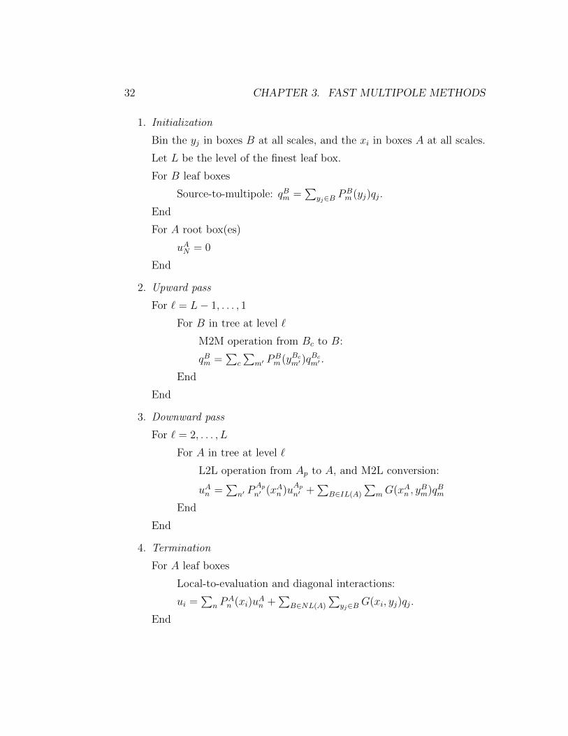
32 CHAPTER 3. FAST MULTIPOLE METHODS
1. Initialization
Bin the yj in boxes B at all scales, and the xi in boxes A at all scales.
Let L be the level of the finest leaf box.
For B leaf boxes
Source-to-multipole: qBm =∑
yj∈B PBm (yj)qj.
End
For A root box(es)
uAN = 0
End
2. Upward pass
For ` = L− 1, . . . , 1
For B in tree at level `
M2M operation from Bc to B:
qBm =∑
c
∑m′ P
Bm (yBc
m′ )qBc
m′ .
End
End
3. Downward pass
For ` = 2, . . . , L
For A in tree at level `
L2L operation from Ap to A, and M2L conversion:
uAn =∑
n′ PAp
n′ (xAn )uAp
n′ +∑
B∈IL(A)
∑mG(xAn , y
Bm)qBm
End
End
4. Termination
For A leaf boxes
Local-to-evaluation and diagonal interactions:
ui =∑
n PAn (xi)u
An +
∑B∈NL(A)
∑yj∈B G(xi, yj)qj.
End
3.3. THE FAST MULTIPOLE METHOD 33
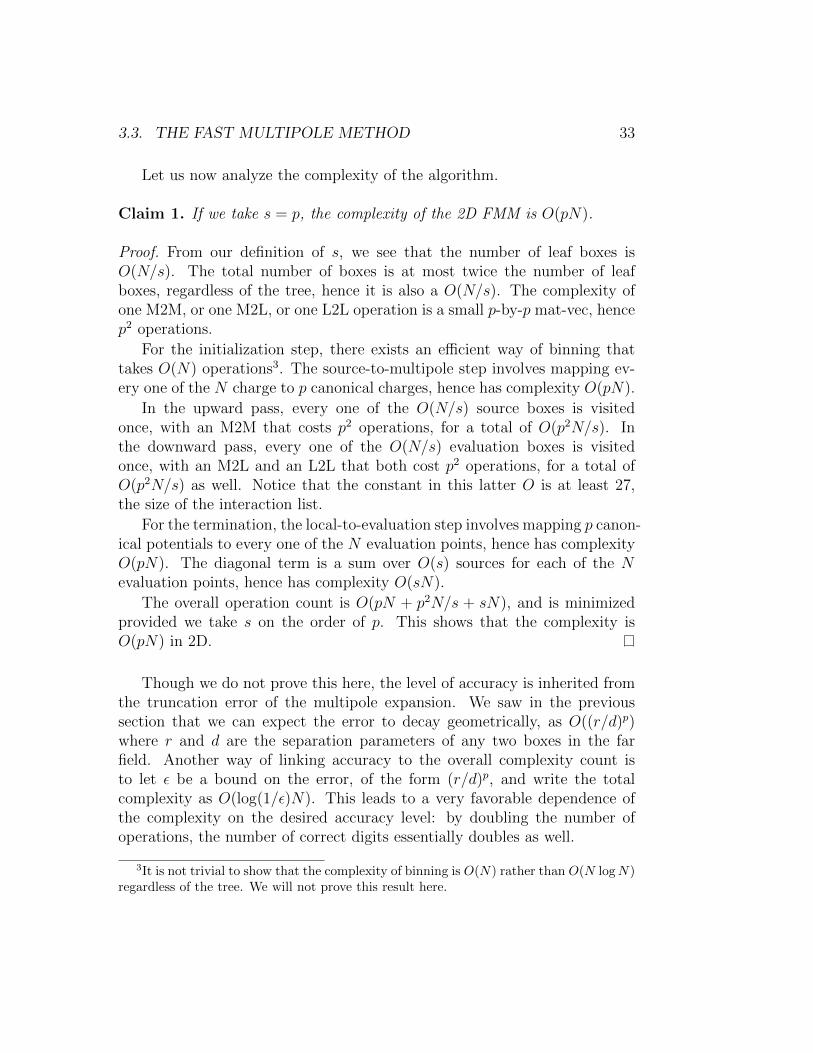
Let us now analyze the complexity of the algorithm.
Claim 1. If we take s = p, the complexity of the 2D FMM is O(pN).
Proof. From our definition of s, we see that the number of leaf boxes isO(N/s). The total number of boxes is at most twice the number of leafboxes, regardless of the tree, hence it is also a O(N/s). The complexity ofone M2M, or one M2L, or one L2L operation is a small p-by-p mat-vec, hencep2 operations.
For the initialization step, there exists an efficient way of binning thattakes O(N) operations3. The source-to-multipole step involves mapping ev-ery one of the N charge to p canonical charges, hence has complexity O(pN).
In the upward pass, every one of the O(N/s) source boxes is visitedonce, with an M2M that costs p2 operations, for a total of O(p2N/s). Inthe downward pass, every one of the O(N/s) evaluation boxes is visitedonce, with an M2L and an L2L that both cost p2 operations, for a total ofO(p2N/s) as well. Notice that the constant in this latter O is at least 27,the size of the interaction list.
For the termination, the local-to-evaluation step involves mapping p canon-ical potentials to every one of the N evaluation points, hence has complexityO(pN). The diagonal term is a sum over O(s) sources for each of the Nevaluation points, hence has complexity O(sN).
The overall operation count is O(pN + p2N/s + sN), and is minimizedprovided we take s on the order of p. This shows that the complexity isO(pN) in 2D.
Though we do not prove this here, the level of accuracy is inherited fromthe truncation error of the multipole expansion. We saw in the previoussection that we can expect the error to decay geometrically, as O((r/d)p)where r and d are the separation parameters of any two boxes in the farfield. Another way of linking accuracy to the overall complexity count isto let ε be a bound on the error, of the form (r/d)p, and write the totalcomplexity as O(log(1/ε)N). This leads to a very favorable dependence ofthe complexity on the desired accuracy level: by doubling the number ofoperations, the number of correct digits essentially doubles as well.
3It is not trivial to show that the complexity of binning is O(N) rather than O(N logN)regardless of the tree. We will not prove this result here.
34 CHAPTER 3. FAST MULTIPOLE METHODS
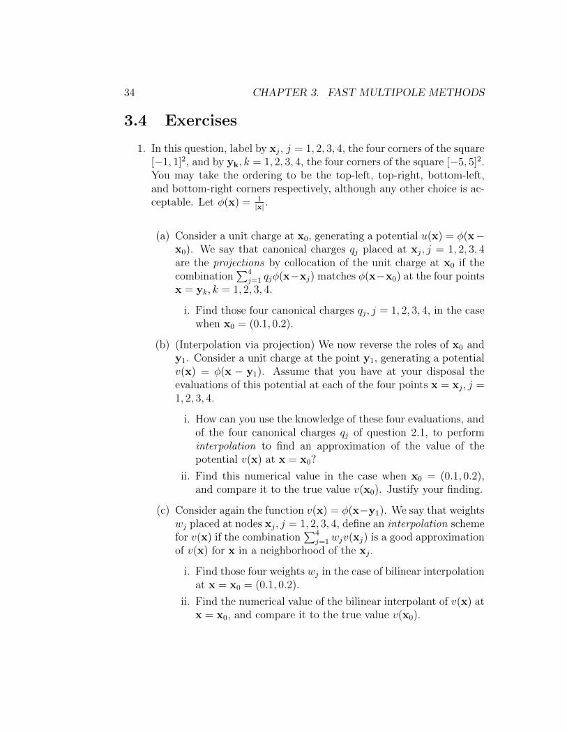
3.4 Exercises
1. In this question, label by xj, j = 1, 2, 3, 4, the four corners of the square[−1, 1]2, and by yk, k = 1, 2, 3, 4, the four corners of the square [−5, 5]2.You may take the ordering to be the top-left, top-right, bottom-left,and bottom-right corners respectively, although any other choice is ac-ceptable. Let φ(x) = 1
|x| .
(a) Consider a unit charge at x0, generating a potential u(x) = φ(x−x0). We say that canonical charges qj placed at xj, j = 1, 2, 3, 4are the projections by collocation of the unit charge at x0 if thecombination
∑4j=1 qjφ(x−xj) matches φ(x−x0) at the four points
x = yk, k = 1, 2, 3, 4.
i. Find those four canonical charges qj, j = 1, 2, 3, 4, in the casewhen x0 = (0.1, 0.2).
(b) (Interpolation via projection) We now reverse the roles of x0 andy1. Consider a unit charge at the point y1, generating a potentialv(x) = φ(x − y1). Assume that you have at your disposal theevaluations of this potential at each of the four points x = xj, j =1, 2, 3, 4.
i. How can you use the knowledge of these four evaluations, andof the four canonical charges qj of question 2.1, to performinterpolation to find an approximation of the value of thepotential v(x) at x = x0?
ii. Find this numerical value in the case when x0 = (0.1, 0.2),and compare it to the true value v(x0). Justify your finding.
(c) Consider again the function v(x) = φ(x−y1). We say that weightswj placed at nodes xj, j = 1, 2, 3, 4, define an interpolation schemefor v(x) if the combination
∑4j=1wjv(xj) is a good approximation
of v(x) for x in a neighborhood of the xj.
i. Find those four weights wj in the case of bilinear interpolationat x = x0 = (0.1, 0.2).
ii. Find the numerical value of the bilinear interpolant of v(x) atx = x0, and compare it to the true value v(x0).
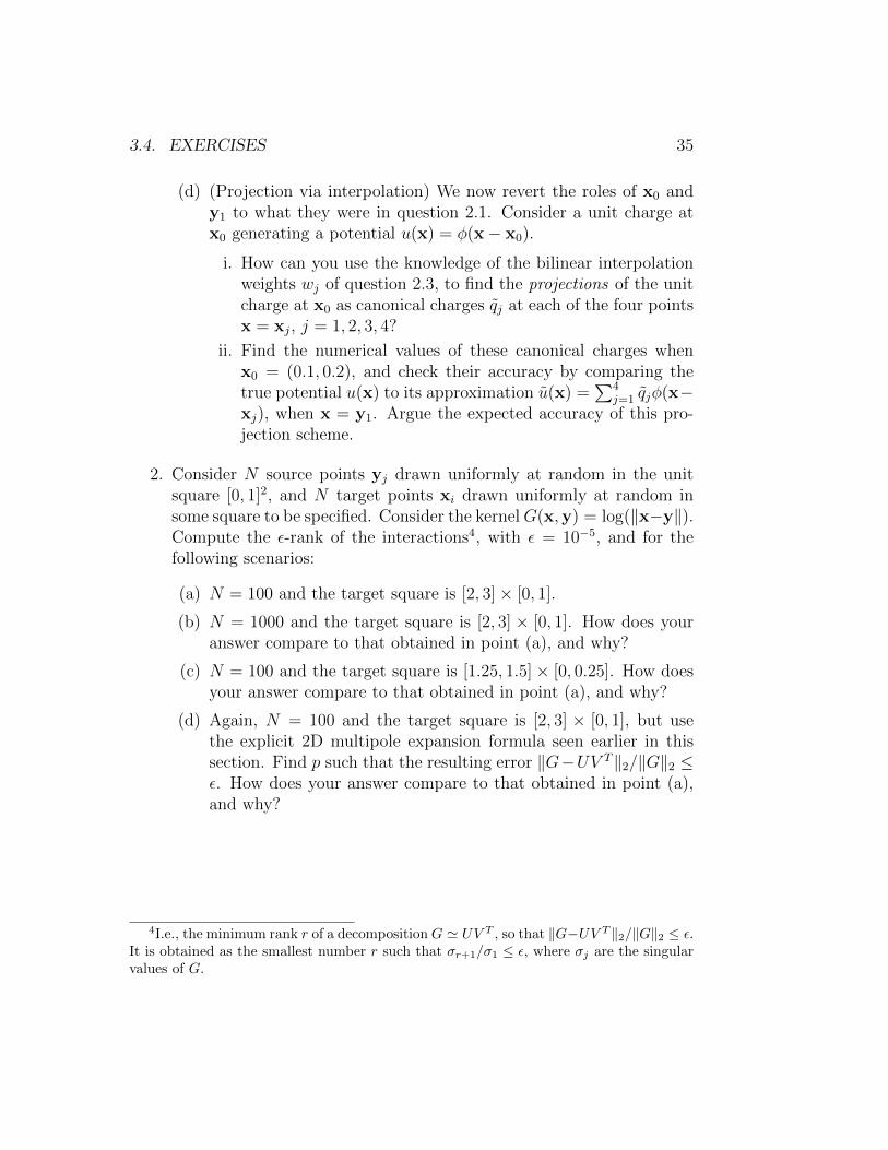
3.4. EXERCISES 35
(d) (Projection via interpolation) We now revert the roles of x0 andy1 to what they were in question 2.1. Consider a unit charge atx0 generating a potential u(x) = φ(x− x0).
i. How can you use the knowledge of the bilinear interpolationweights wj of question 2.3, to find the projections of the unitcharge at x0 as canonical charges qj at each of the four pointsx = xj, j = 1, 2, 3, 4?
ii. Find the numerical values of these canonical charges whenx0 = (0.1, 0.2), and check their accuracy by comparing thetrue potential u(x) to its approximation u(x) =
∑4j=1 qjφ(x−
xj), when x = y1. Argue the expected accuracy of this pro-jection scheme.
2. Consider N source points yj drawn uniformly at random in the unitsquare [0, 1]2, and N target points xi drawn uniformly at random insome square to be specified. Consider the kernelG(x,y) = log(‖x−y‖).Compute the ε-rank of the interactions4, with ε = 10−5, and for thefollowing scenarios:
(a) N = 100 and the target square is [2, 3]× [0, 1].
(b) N = 1000 and the target square is [2, 3] × [0, 1]. How does youranswer compare to that obtained in point (a), and why?
(c) N = 100 and the target square is [1.25, 1.5]× [0, 0.25]. How doesyour answer compare to that obtained in point (a), and why?
(d) Again, N = 100 and the target square is [2, 3] × [0, 1], but usethe explicit 2D multipole expansion formula seen earlier in thissection. Find p such that the resulting error ‖G−UV T‖2/‖G‖2 ≤ε. How does your answer compare to that obtained in point (a),and why?
4I.e., the minimum rank r of a decomposition G ' UV T , so that ‖G−UV T ‖2/‖G‖2 ≤ ε.It is obtained as the smallest number r such that σr+1/σ1 ≤ ε, where σj are the singularvalues of G.

36 CHAPTER 3. FAST MULTIPOLE METHODS
Chapter 4
Hierarchical matrices
This chapter details the linear algebraic point of view behind partitionedlow-rank matrices, the fast multipole method, and the calculus of hierarchialmatrices.
4.1 Low-rank decompositions
In this section we discuss the linear algebraic context of the projection andinterpolation operations, and their generalizations.
Let us return to the case of x ∈ A and y ∈ B, with A and B well-separated, so we are in effect considering an off-diagonal block of G (but stillcontinue to write it G ouf of convenience). The variable x is viewed as a(possibly continuous) row index, while y is a (possibly continuous) columnindex. A low-rank expansion of G is any expression where x vs. y appear inseparated factors, of the form
G(x, y) =∑m,n
Un(x)SnmVm(y), G = USV T
It is often useful to limit the ranges of m and n to 1 ≤ m,n ≤ p, whichresults in a numerical error ε:
‖G(x, y)−P∑
m,n=1
Un(x)SnmVm(y)‖ ≤ ε. (4.1)
The ε-rank of G is the smallest p for which (4.1) holds with the spectral(induced `2) norm. The optimal factors U, S, and V , for which the separationerror is smallest, are given by the singular value decomposition.
37
38 CHAPTER 4. HIERARCHICAL MATRICES
There are, however, other ways to perform low-rank decompositions thathave different redeeming features. Consider the single-charge projection re-lation (3.2), namely
G(x, yj) '∑m
G(x, yBm)QBm(yj), x ∈ A, yj ∈ B,
In the case when the yBm are taken as a subset of the original points yj, therelation can be read as a low-rank decomposition
G ' GcQT ,
where Gc is a tall-and-thin column restriction of G, and Q is the matrixgenerated by the projection rule.
Conversely, when xAn form a subset of the xi, the single-charge interpola-tion condition (3.5) can be read as the low-rank decomposition
G ' PGr,
where Gr is now a short-and-wide row restriction of G, and P is the matrixgenerated by the interpolation rule. Recall that (i) G is symmetic, (ii) wemay take P = Q, and (iii) the same subset of points can be used to generatethe rows of Gr and the columns of Gc, hence the projection and interpolationdecompositions are truly transposes of one another.
The low-rank decompositions generated from projection and interpolationare simply called interpolative decompositions. They interesting in their ownright, for two reasons: 1) the factors Gc and Gr only require evaluations ofthe kernel: if an explicit formula or an on-demand evaluation function isavailable for that kernel, the storage requirement for P and/or Q is muchlighter than that of the three factors U , S, and V T ; and 2) the matrix Pis independent of the box B that defines the column-restriction of G, andsimilarly QT is independent of the box A that defines the row restrictionof G, hence such interpolative decompositions can often be re-used acrossboxes.
We have already seen examples of Q that can be used in a projectiondecomposition G ' GcQ
T . The linear algebra point of view invites to chooseQ as the solution of an overdetermined least-squares problem of the form
QT = G+c G,
4.1. LOW-RANK DECOMPOSITIONS 39
but only after the Gc and G matrices are properly restricted in x, their rowindex. One could for instance let x run over the sequence xi: this results in aprojection rule that is often at best valid near the convex hull of the points xi.In particular, the projection rule would need to change if the evaluation boxA is changed. A much better choice is the collocation rule seen previously,which uses check points xi on a check surface surrounding B: the resultingprojection rule is now independent of the evaluation box and will work assoon as the evaluation point is outside the check surface. But notice that wehad to lift the restriction x ∈ A in the collocation scheme, hence we had tolook outside of the linear algebra framework to find the better solution!
As for the column restriction that takes G to Gc, many choices are pos-sible. Linear algebra offers an interesting solution: the columns (at yBm) thattake part in Gc can be picked from the columns (at yj) of G by a rank-revealing QR decomposition1. Cheaper methods exist for selecting thesecolumns, such as random sampling, or adaptive cross-approximation (ACA).We also saw in the previous section that we can pick the yBm as the nodes ofa polynomial interpolation scheme, though this results in points that may beoutside of the original collection yj – a solution which again operates outsidea strict linear algebra framework.
Another useful low-rank decomposition of G is the so-called CUR form,or skeleton form, written as
G ' GcZGr,
where the middle matrix Z is chosen for the approximation to be good. Thebest choice in the least-squares (Frobenius) sense is Z = G+
c GG+r , which
again requires collocation to properly row-restrict G and Gc; and column-restrict G and Gr. A convenient but suboptimal choice is Z = G+
cr whereGcr is the row and column restriction of G corresponding to the same indexsets that define Gc and Gr. We can compare the different factorizations of Gto conclude that we may define “skeleton” projection and interpolation rulesvia
QT = ZGr, P = GcZ.
1The letter Q is already taken, so write G = UR for the thin QR decomposition.Because of pivoting, R is not necessarily lower triangular. Now extract from G the exactsame columns that were orthogonalized in the process of forming U , and call the resultGc. Write Gc = URc with Rc a square, invertible matrix. Then G = GcR
−1c R = GcQ
with Q = R−1c R.
40 CHAPTER 4. HIERARCHICAL MATRICES
The most useful aspect of the low rank point of view is that it is universal,i.e., it informs the feasibility of projection and interpolation regardless of theparticular method used.
1. If there exists a rank-r factorization of G into UV T , then there mustexist a factorization G = GcQ
T using r columns of G. In particular,a projection rule incurs no penalty2 if the yBm are chosen among theyj points (the interpolative case) rather than outside of this collection(the extrapolative case).
2. The availabilty of efficient projection and interpolation rules cruciallyhinges on the separability of the kernel G restricted to source and eval-uation boxes. If the ε-rank of a block of G is greater than r, thenthere does not exist a projection rule with r canonical charges, or aninterpolation rule with r canonical potentials, that could ever reach anerror smaller than ε (in an `2 sense).
We already saw a justification of the separability of the A×B block of Gin the multipole section. Let us now argue, from an algebraic argumentin 1D, that we can expect low rank for off-diagonal blocks of inverse ofbanded matrices. Consider a finite difference discretization of a boundary-value ODE, leading to
T =
α1 β1
γ1 α2. . .
. . . . . . βn−1
γn−1 αn
Let G = T−1, i.e., G is the so-called Green’s matrix corresponding to a3-point finite difference stencil.
Theorem 2. Assume T is tridiagonal and invertible. Then G = T−1 hasrank-1 off-diagonal blocks.
2There is truly no penalty if the rank is exactly r, and in exact arithmetic. There isa minor factor
√rn in loss of accuracy for truncation to r separated components by a
QR decomposition, or in our notations GcQT , over an SVD if the rank is not exactly r,
however.
4.2. CALCULUS OF HIERARCHICAL MATRICES 41
Proof. Fix j, and consider that
T = U + βjejeTj ,
where U is T with its βj element put to zero, and ej is the j-th canonicalbasis vector in Rn. Notice that U is upper block-triangular with a block ofzeros in positions [1 : j]× [(j+ 1) : n]. Since the inverse of a block-triangularmatrix is also block-triangular, U−1 also has a block of zeros in positions[1 : j] × [(j + 1) : n]. To obtain T−1, apply the Woodbury formula, whichshows that T−1 differs from U−1 by a rank-1 matrix:
T−1 = U−1 −(U−1ej)(e
Tj+1U
−1)
1 + βjeTj+1U−1ej
.
(The scalar denominator is nonzero because T−1 is invertible.) Hence theblock [1 : j]× [(j + 1) : n] of T−1 has rank 1. An analogous argument showsthat the block [(j + 1) : n]× [1 : j] also has rank 1.
More generally, if T has band width 2p+ 1, i.e., p upper diagonals and plower diagonals, then the rank of the off-diagonal blocks of T−1 is p.
A matrix whose off-diagonal blocks have rank p is called p-semiseparable.For each p, tshe set of invertible p-semiseparable matrices is closed underinversion (unlike the set of tridiagonal matrices, for instance).
[Extension to blocks]
4.2 Calculus of hierarchical matrices
4.3 Hierarchical matrices meet the FMM

42 CHAPTER 4. HIERARCHICAL MATRICES
Chapter 5
Butterfly algorithms
Butterfly algorithms are helpful for computing oscillatory sums arising inthe high-frequency wave propagation context. We now consider a large wavenumber k, and kernels such as the fundamental solution of the Helmholtzequation in 3D,
G(x, y) =eik|x−y|
4π|x− y|,
or its counterpart in 2D, G(x, y) = i4H
(1)0 (k|x − y|). The wave number is
related to the angular frequency ω and the wave speed c via the dispersionrelation ω = kc.
5.1 Separation in the high-frequency regime
For high-frequency scattering and other oscillatory kernels, we have goodseparation if the boxes A and B
diam(A)× diam(B) . d(A,B)× λ,
where d(A,B) is the distance between box centers, and λ = 2π/k is thewavelength.
5.2 Architecture of the butterfly algorithm
The separation condition is much more restrictive in the high-frequency case,prompting the introduction of a different “butterfly” algorithm:
43
44 CHAPTER 5. BUTTERFLY ALGORITHMS
• The check potentials are split into different contributions coming fromdifferent sources boxes, and denoted uABn ; and
• The equivalent densities are split into different contributions generatingpotentials in different target boxes, and denoted qABm .
The interpolation rules are now valid only for x ∈ A and y ∈ B. Theinterpolation basis functions depend both on A and on B, and are denotedPABn (x).
• An interpolation rule in the x variable,
G(x, y) =∑n
PABn (x)G(xAn , y), x ∈ A, y ∈ B, (5.1)
generates a notion of local expansion. Consider check potentials uABnat the nodes xAn ,
uABn =
∫B
G(xAn , y)q(y)dy. (5.2)
The interpolation rule in x allows to switch from potentials at xAn topotentials everywhere in A: combine (3.14), (5.1), (5.2) to get
uB(x) =∑n
PABn (x)uABn , x ∈ A. (5.3)
• An interpolation rule in the y variable,
G(x, y) =∑m
G(x, yBm)PABm (y), x ∈ A, y ∈ B, (5.4)
generates a notion of multipole (interpolative) expansion. Considerequivalent densities qABm at the nodes yBm, so that
uB(x) =∑m
G(x, yBm)qABm , x ∈ A. (5.5)
The interpolation rule in y allows to switch from densities in B toequivalent densities qBm: combine (3.14), (5.4), (5.5) to get
qABm =
∫B
PABm (y)q(y)dy. (5.6)
5.2. ARCHITECTURE OF THE BUTTERFLY ALGORITHM 45
We say that a couple (A,B) is admissible when the boxes are well-separated in the sense explained in the previous section.
The condition on the admissibility of couples of boxes determines theform of an L2L operation:
uABn +=∑c
∑n′
PApBc
n′ (xAn )uApBc
n′ .
An M2M operation is
qABm =∑c
∑m′
PABm (yBc
m′ )qApBc
m′ .
An M2L conversion is
uAB↑
n +=∑m
G(xAn , yBm)qA
↑Bm ,
where B is in the interaction list of A. There is no sum to perform over theinteraction list. The notation A↑ refers to some ancestor of A; this precautionarises from the fact that we want A and B on the same level for the M2Ltranslation, but the uABn and qABm are usually available only for boxes atdifferent levels (B at a higher level than A for u and B at a lower level thanA for q).
The choice of interpolation scheme may be dictated by the particularkernel. An all-purpose choice is to use translated copies of the kernel itself:
PABn (x) =
∑m
G(x, yBm)dABmn .
A substitution in (5.1) reveals that the d coefficients are obtained as themiddle factor of a skeleton decomposition of the (A,B) block of G,
G(x, y) =∑m,n
G(x, yBm)dABmnG(xAn , y).

46 CHAPTER 5. BUTTERFLY ALGORITHMS
Appendix A
The Fast Fourier transform(FFT)
47

48 APPENDIX A. THE FAST FOURIER TRANSFORM (FFT)
Appendix B
Linear and cyclic convolutions
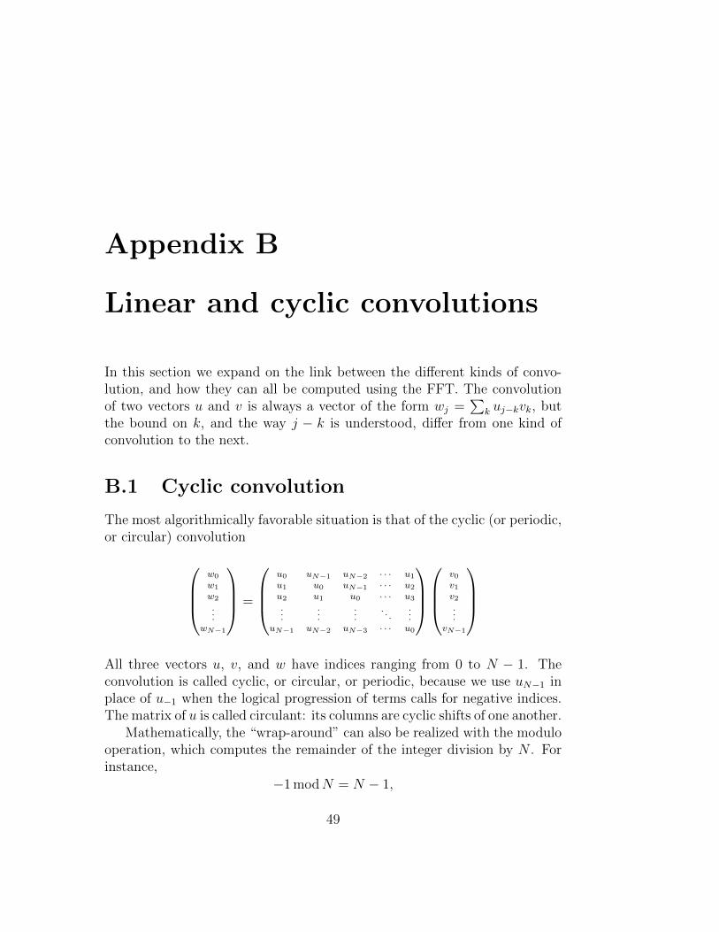
In this section we expand on the link between the different kinds of convo-lution, and how they can all be computed using the FFT. The convolutionof two vectors u and v is always a vector of the form wj =
∑k uj−kvk, but
the bound on k, and the way j − k is understood, differ from one kind ofconvolution to the next.
B.1 Cyclic convolution
The most algorithmically favorable situation is that of the cyclic (or periodic,or circular) convolution
w0
w1
w2
...wN−1
=
u0 uN−1 uN−2 · · · u1u1 u0 uN−1 · · · u2u2 u1 u0 · · · u3...
......
. . ....
uN−1 uN−2 uN−3 · · · u0
v0v1v2...
vN−1
All three vectors u, v, and w have indices ranging from 0 to N − 1. Theconvolution is called cyclic, or circular, or periodic, because we use uN−1 inplace of u−1 when the logical progression of terms calls for negative indices.The matrix of u is called circulant: its columns are cyclic shifts of one another.
Mathematically, the “wrap-around” can also be realized with the modulooperation, which computes the remainder of the integer division by N . Forinstance,
−1 modN = N − 1,
49
50 APPENDIX B. LINEAR AND CYCLIC CONVOLUTIONS
0 modN = 0
(N − 1) modN = N − 1,
N modN = 0,
(N + 1) modN = 1,
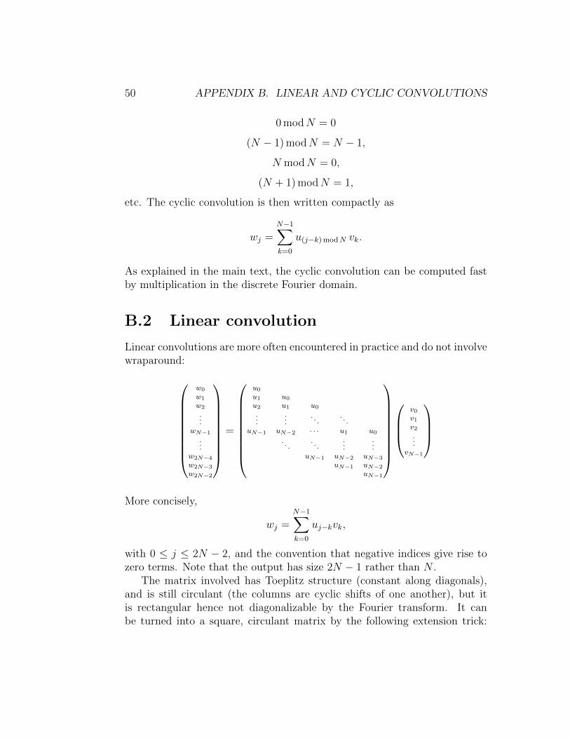
etc. The cyclic convolution is then written compactly as
wj =N−1∑k=0
u(j−k) modN vk.
As explained in the main text, the cyclic convolution can be computed fastby multiplication in the discrete Fourier domain.
B.2 Linear convolution
Linear convolutions are more often encountered in practice and do not involvewraparound:
w0
w1
w2
...wN−1
...w2N−4
w2N−3
w2N−2
=
u0u1 u0u2 u1 u0...
.... . .
. . .
uN−1 uN−2 · · · u1 u0. . .
. . ....
...uN−1 uN−2 uN−3
uN−1 uN−2
uN−1
v0v1v2...
vN−1
More concisely,
wj =N−1∑k=0
uj−kvk,
with 0 ≤ j ≤ 2N − 2, and the convention that negative indices give rise tozero terms. Note that the output has size 2N − 1 rather than N .
The matrix involved has Toeplitz structure (constant along diagonals),and is still circulant (the columns are cyclic shifts of one another), but itis rectangular hence not diagonalizable by the Fourier transform. It canbe turned into a square, circulant matrix by the following extension trick:
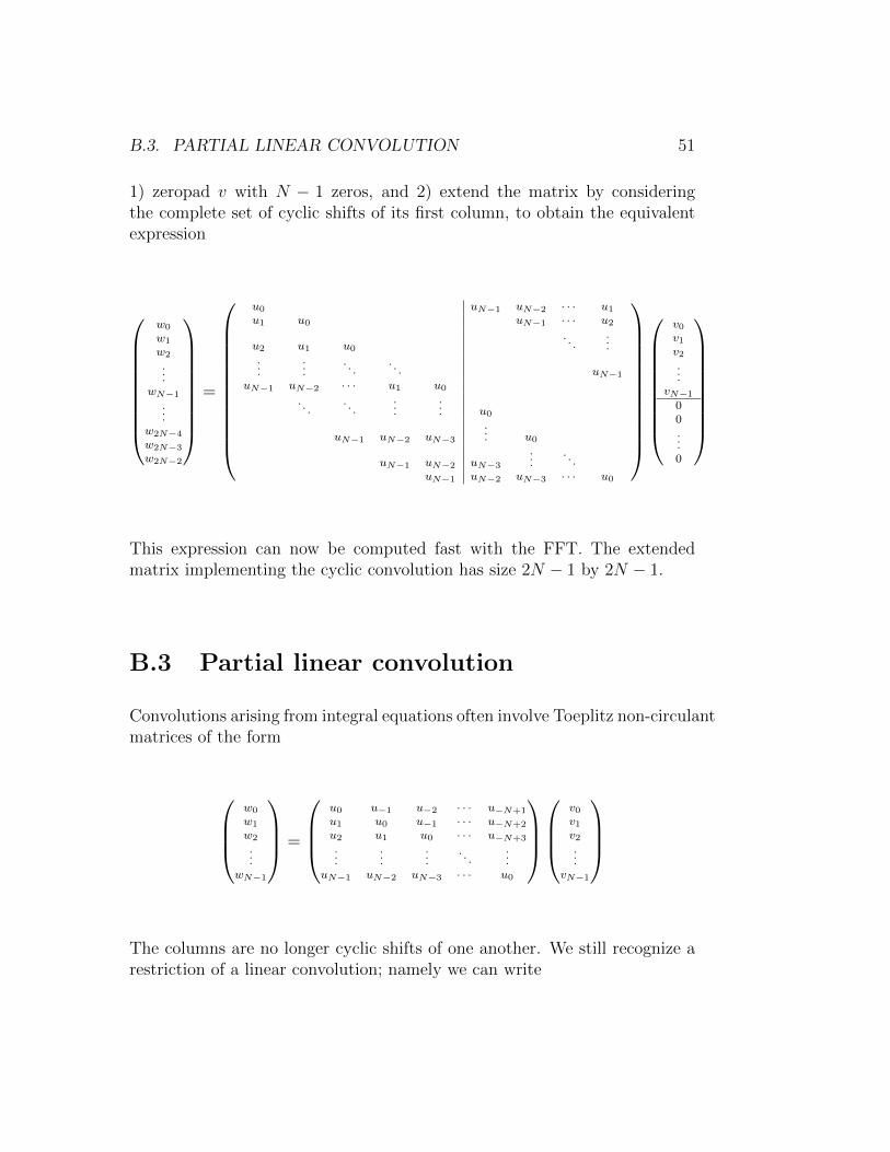
B.3. PARTIAL LINEAR CONVOLUTION 51
1) zeropad v with N − 1 zeros, and 2) extend the matrix by consideringthe complete set of cyclic shifts of its first column, to obtain the equivalentexpression
w0
w1
w2
...wN−1
...w2N−4
w2N−3
w2N−2
=
u0 uN−1 uN−2 · · · u1u1 u0 uN−1 · · · u2
u2 u1 u0. . .
......
.... . .
. . . uN−1
uN−1 uN−2 · · · u1 u0. . .
. . ....
... u0
uN−1 uN−2 uN−3
... u0
uN−1 uN−2 uN−3
.... . .
uN−1 uN−2 uN−3 · · · u0
v0v1v2...
vN−1
00...0
This expression can now be computed fast with the FFT. The extendedmatrix implementing the cyclic convolution has size 2N − 1 by 2N − 1.
B.3 Partial linear convolution
Convolutions arising from integral equations often involve Toeplitz non-circulantmatrices of the form
w0
w1
w2
.
..wN−1
=
u0 u−1 u−2 · · · u−N+1
u1 u0 u−1 · · · u−N+2
u2 u1 u0 · · · u−N+3
......
.... . .
...uN−1 uN−2 uN−3 · · · u0
v0v1v2...
vN−1
The columns are no longer cyclic shifts of one another. We still recognize arestriction of a linear convolution; namely we can write
52 APPENDIX B. LINEAR AND CYCLIC CONVOLUTIONS
××...×w0
w1
...wN−2
wN−1
×...××
=
u−N+1
u−N+2 u−N+1
......
. . .
u−1 u−2 · · · u−N+1
u0 u−1 · · · u−N+2 u−N+1
u1 u0 · · · u−N+3 u−N+2
......
. . ....
...uN−2 uN−3 · · · u0 u−1
uN−1 uN−2 · · · u1 u0uN−1 · · · u2 u1
. . ....
...uN−1 uN−2
uN−1
v0v1v2...
vN−1
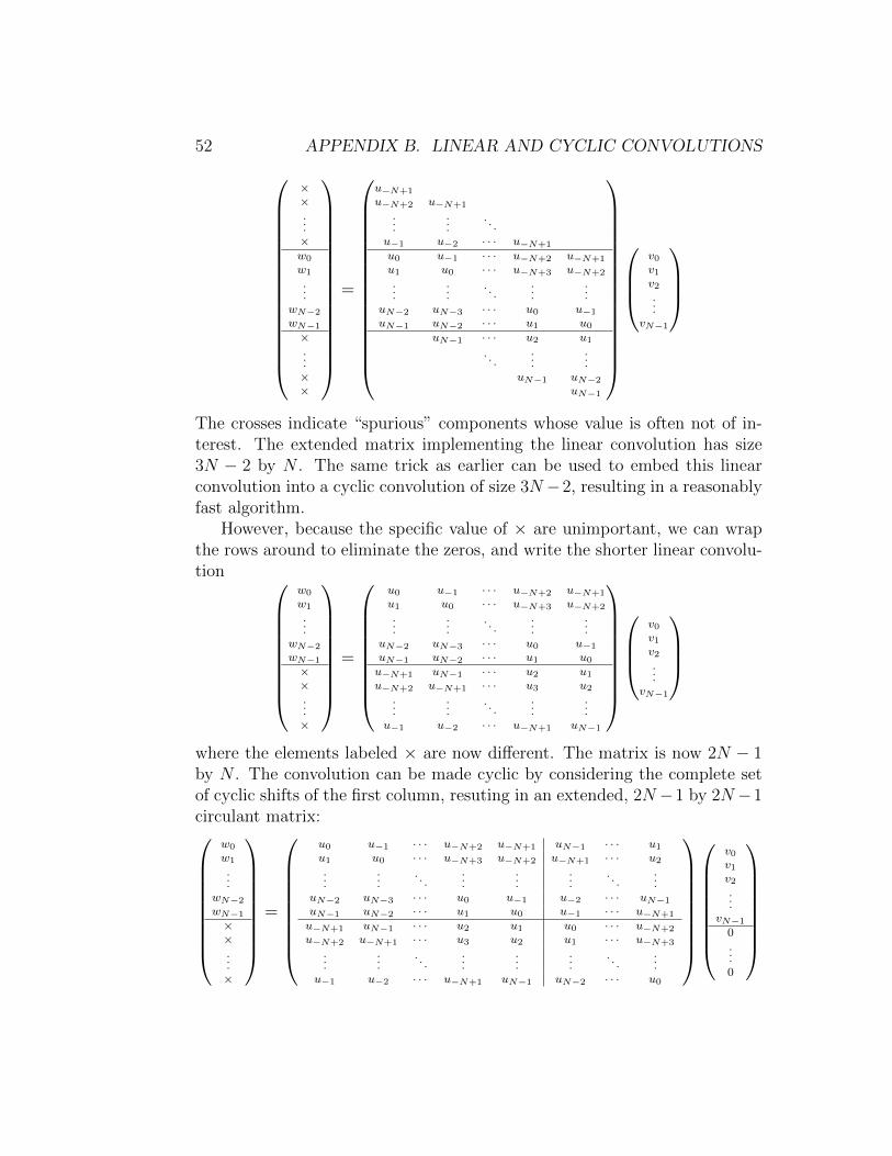
The crosses indicate “spurious” components whose value is often not of in-terest. The extended matrix implementing the linear convolution has size3N − 2 by N . The same trick as earlier can be used to embed this linearconvolution into a cyclic convolution of size 3N−2, resulting in a reasonablyfast algorithm.
However, because the specific value of × are unimportant, we can wrapthe rows around to eliminate the zeros, and write the shorter linear convolu-tion
w0
w1
...wN−2
wN−1
××...×
=
u0 u−1 · · · u−N+2 u−N+1
u1 u0 · · · u−N+3 u−N+2
......
. . ....
...uN−2 uN−3 · · · u0 u−1
uN−1 uN−2 · · · u1 u0u−N+1 uN−1 · · · u2 u1u−N+2 u−N+1 · · · u3 u2
......
. . ....
...u−1 u−2 · · · u−N+1 uN−1
v0v1v2...
vN−1
where the elements labeled × are now different. The matrix is now 2N − 1by N . The convolution can be made cyclic by considering the complete setof cyclic shifts of the first column, resuting in an extended, 2N−1 by 2N−1circulant matrix:
w0
w1
...wN−2
wN−1
××...×
=
u0 u−1 · · · u−N+2 u−N+1 uN−1 · · · u1u1 u0 · · · u−N+3 u−N+2 u−N+1 · · · u2...
.... . .
......
.... . .
...uN−2 uN−3 · · · u0 u−1 u−2 · · · uN−1
uN−1 uN−2 · · · u1 u0 u−1 · · · u−N+1
u−N+1 uN−1 · · · u2 u1 u0 · · · u−N+2
u−N+2 u−N+1 · · · u3 u2 u1 · · · u−N+3
..
....
. . ....
......
. . ....
u−1 u−2 · · · u−N+1 uN−1 uN−2 · · · u0
v0v1v2...
vN−1
0...0
B.4. PARTIAL, SYMMETRIC LINEAR CONVOLUTION 53
The prescription for a fast algorithm is therefore to consider the first column,
(u0, u1, . . . , uN−1, u−N+1, . . . , u−1)T ,
and perform its cyclic convolution with the zeropadded vector v. This variantis more efficient by roughly 50% than the 3N − 2 by 3N − 2 formulationdescribed earlier.
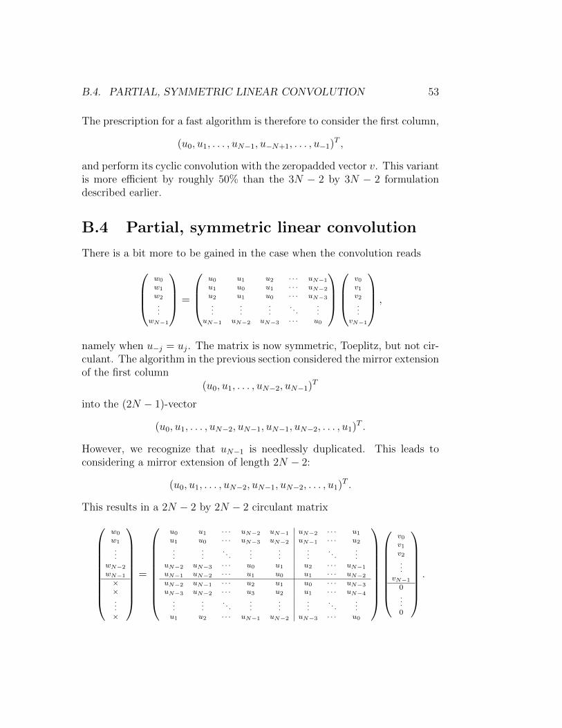
B.4 Partial, symmetric linear convolution
There is a bit more to be gained in the case when the convolution readsw0
w1
w2
...wN−1
=
u0 u1 u2 · · · uN−1
u1 u0 u1 · · · uN−2
u2 u1 u0 · · · uN−3
......
.... . .
...uN−1 uN−2 uN−3 · · · u0
v0v1v2...
vN−1
,
namely when u−j = uj. The matrix is now symmetric, Toeplitz, but not cir-culant. The algorithm in the previous section considered the mirror extensionof the first column
(u0, u1, . . . , uN−2, uN−1)T
into the (2N − 1)-vector
(u0, u1, . . . , uN−2, uN−1, uN−1, uN−2, . . . , u1)T .
However, we recognize that uN−1 is needlessly duplicated. This leads toconsidering a mirror extension of length 2N − 2:
(u0, u1, . . . , uN−2, uN−1, uN−2, . . . , u1)T .
This results in a 2N − 2 by 2N − 2 circulant matrix
w0
w1
...wN−2
wN−1
××...×
=
u0 u1 · · · uN−2 uN−1 uN−2 · · · u1u1 u0 · · · uN−3 uN−2 uN−1 · · · u2...
.... . .
......
.... . .
...uN−2 uN−3 · · · u0 u1 u2 · · · uN−1
uN−1 uN−2 · · · u1 u0 u1 · · · uN−2
uN−2 uN−1 · · · u2 u1 u0 · · · uN−3
uN−3 uN−2 · · · u3 u2 u1 · · · uN−4
..
....
. . ....
......
. . ....
u1 u2 · · · uN−1 uN−2 uN−3 · · · u0
v0v1v2...
vN−1
0...0
.

54 APPENDIX B. LINEAR AND CYCLIC CONVOLUTIONS
Whether the FFT-based algorithm for matrix-vector multiplication is nowfaster than the variant seen in the previous section depends on whether 2N−2is “more composite” than 2N − 1 (which it stands a better chance of being,by virtue of being even). With additional zeropadding, it is simple to imaginevariants with 2N by 2N or larger matrices.


