Abstract GNSS ambiguity resolution is the key issue in thehigh-precision relative geodetic positioning and navigationapplications. It is a problem of integer programming plusinteger quality evaluation. Different integer search estima-tion methods have been proposed for the integer solution ofambiguity resolution. Slow rate of convergence is the mainobstacle to the existing methods where tens of ambiguitiesare involved. Herein, integer search estimation for the GNSSambiguity resolution based on the lattice theory is proposed.It is mathematically shown that the closest lattice point prob-lem is the same as the integer least-squares (ILS) estimationproblem and that the lattice reduction speeds up searchingprocess. We have implemented three integer search strate-gies: Agrell, Eriksson, Vardy, Zeger (AEVZ), modificationof Schnorr–Euchner enumeration (M-SE) and modificationof Viterbo-Boutros enumeration (M-VB). The methods havebeen numerically implemented in several simulated exam-ples under different scenarios and over 100 independentruns. The decorrelation process (or unimodular transforma-tions) has been first used to transform the original ILS prob-lem to a new one in all simulations. We have then applied
Electronic supplementary material The online version of thisarticle (doi:10.1007/s00190-011-0501-z) contains supplementarymaterial, which is available to authorized users.
S. Jazaeri (B) · M. A. SharifiDepartment of Surveying and Geomatics Engineering,College of Engineering, University of Tehran, Tehran, Irane-mail: [email protected]
A. R. Amiri-SimkooeiDepartment of Surveying Engineering, Faculty of Engineering,University of Isfahan, 81746-73441 Isfahan, Irane-mail: [email protected]
different search algorithms to the transformed ILS prob-lem. The numerical simulations have shown that AEVZ,M-SE, and M-VB are about 320, 120 and 50 times fasterthan LAMBDA, respectively, for a search space of dimen-sion 40. This number could change to about 350, 160 and60 for dimension 45. The AEVZ is shown to be faster thanMLAMBDA by a factor of 5. Similar conclusions could bemade using the application of the proposed algorithms to thereal GPS data.
High-precision GNSS positioning is achieved using the car-rier phase observables in the relative positioning mode.GNSS relative positioning is used for many high-precisionapplications such as surveying, mapping, GIS, and precisenavigation. A prerequisite to this is the successful determina-tion of the integer double difference carrier phase ambiguityparameters. Mathematically, double difference carrier phaseobservation equation is a mixed integer nonlinear model. Lin-earizing the carrier phase observation equation yields the fol-lowing mixed integer linear model (Teunissen 1995; Xu et al.1995; Xu 2006):
y = Aa + Bb + e (1)
where y is a t-dimensional vector of observed minus approx-imate double difference carrier phase observations, a is ann-dimensional integer vector, b is an m-dimensional real-val-ued vector, e is the error vector of observations, and A and Bare the t × n and t × m real-valued matrices, respectively.
Fig. 1 Some of carrier phaseambiguity resolution methodsavailable in literature
Applying the least-squares criterion to (1), to estimate theunknown parameters, yields
min(y − Aa − Bb)TP(y − Aa − Bb) (2)
where P is the weight matrix of observables. This minimi-zation problem, which is a type of mixed integer nonlin-ear programming (MINLP) problem, is also referred to asa mixed integer least-squares (ILS) problem. The ambiguityparameters are initially determined as part of the ordinaryleast-squares by neglecting the integerness of ambiguities.
What can be obtained are the real-valued parameters
([ab
])
along with their covariance matrix
([Qa QabQba Qb
]). The
minimization problem in (2) is equivalent to the followingproblem (Teunissen 1993; Xu et al. 1995):
a = min(a − a)TP(a − a) (3)
which is the standard ILS or the integer quadratic program-ming (IQP) problem. It is clear that the solution to the originalmixed ILS problem (2) depends on the solution of ILS (3).Denoting the integer solution of (3) by a, one can then obtainthe least-squares estimates of the real parameters b as
b = (BTPB)−1BTP(y − Aa) (4)
Various methods have been developed in the past to deal withcarrier phase ambiguity resolution. Figure 1 shows some ofthe well known strategies considered so far in literature.
On the whole, ambiguity resolution methods can be clas-sified into two main categories, namely motion-based andsearch-based methods (Buist 2007). Motion-based categorytakes advantage of the information contained in the changesin visible GNSS satellites or the motion of the platform, i.e.changes in receiver-satellite geometry. This motion-basedmethod takes time to ambiguity solution and requires at leastthree non-coplanar baselines (Cohen 1996). Therefore, theyare not applicable for real time GNSS positioning and the lat-ter category, i.e. search-based methods are always selectedbecause these methods are not necessarily dependent onmotion.
Search-based methods are classified into three groups:searching in coordinate domain, measurement domain, andambiguity domain. Two types of solutions in ambiguitydomain are called Bayesian and non-Bayesian. There areseveral non-Bayesian methods for ambiguity resolution inambiguity domain. We can at least mention least-squaresambiguity search technique (LSAST) proposed by Lan-gley et al. (1984) and Wei (1986), fast ambiguity res-olution approach (FARA) proposed by Frei and Beutler(1990), least-squares ambiguity decorrelation adjustment(LAMBDA) proposed by Teunissen (1993, 1994, 1995),modified LAMBDA method proposed by Chang et al. (2005),fast ambiguity search filter (FASF) proposed by Chen (1994)and Chen and Lachapelle (1995), integer programming (IP)proposed by Xu et al. (1995) and Xu (1998) and optimalmethod for estimating GPS ambiguities (OMEGA) proposedby Kim and Langley (2000).
In mathematical language, ambiguity resolution is a prob-lem of IP plus integer quality evaluation. We will discussthe first problem in this paper from the point of view of theclosest lattice point (CLP) in lattice theory. The study of lat-tices was originally motivated by the geometry of numbers.A lattice L is a discrete additive subgroup of R
d , gener-ated by the set of integer linear combinations of no morethan d vectors b1, b2, . . ., bk, where k ≤ d. If these vectorsare linearly independent, we say that they are a basis of thelattice L . Lattice basis reduction is the computation of latticebases where the base vectors are not only as orthogonal aspossible to each other, but also as short as possible. This isan important problem in geometry of numbers with appli-cations in communications, combinatorial optimization suchas IP, computer algebra and cryptography (see, for exampleKannan 1987; Steinfeld et al. 2007).
One of the most famous problem related to lattices is theCLP problem: given a lattice basis and a target vector in R
d ,find a lattice vector that is closest to the target. The CLPproblem has applications in various fields, including numbertheory, cryptography and communication theory (Agrell et al.2002). This contribution presents another application of theCLP problem to the problem of integer ambiguity resolution.
123
Fast integer least-squares estimation for GNSS 125
In addition to the US system GPS, the Russian GLONASSis also in place and the European Galileo, Chinese COM-PASS, Japanese QZSS are currently under construction andwill also transmit multiple frequency signals. The increasein satellite availability and transmitted signals will increasethe number of ambiguity parameters. Many methods havebeen developed to increase the search efficiency. However,when dealing with high-dimensional ambiguity parameters,the existing methods are still slow. The goal of this paperis to apply the popular methods taken from the mathemat-ical field of lattice theory to integer search estimation forGNSS ambiguity resolution. We test out these strategies inthe rest of the paper and compare them to the LAMBDA andMLAMBDA methods. Numerical results indicate substantialimprovement in speed to the problem of ILS.
The remaining of this paper is organized as follows. InSect. 2, we introduce the closest point in lattice versus inte-ger ambiguity resolution problem. It is shown how the ILSproblem can be converted to the problem of the closestpoint in the lattice. Section 3 presents the implementationof the lattice theory and mathematically shows lattice basisreduction speeds up searching process. Section 4 gives Pohstand Schnorr–Euchner enumerations. It then presents threesearching closest point algorithms based on the Pohst andSchnorr–Euchner enumerations. We give numerical simu-lated and real GPS experiment results in Sect. 5. Conclusionsare presented in Sect. 6.
2 Lattice theory versus integer ambiguity resolution
2.1 Introduction to lattices
In geometry of numbers, a lattice in Rd is a discrete, addi-
tive, abelian subgroup of Rd consisting of points. Discrete
signifies that there are no cluster points but all points have aminimum Euclidean distance from each other. Let the vectorsb1, b2, . . . , bk ∈ R
d , k ≤ d be linear independent. The set
� ={
u ∈ Rd
∣∣∣∣∣u =k∑
i=1
aibi , ai ∈ Z
}(5)
is called a lattice, where k is the rank of the lattice and d is thedimension of its basis vector. Therefore, every lattice can berepresented by a set B = {b1, b2, . . . , bk} of its basis vectorscalled the basis of the lattice. For a lattice with k = d, werefer to as a full rank lattice. In the matrix form the latticecan be represented as follows:
�(B) = {Ba : a ∈ Zk} (6)
The addition of vectors is associative and commutative, andfurther a lattice is an abelian group. Two lattices with thebasis matrices B and C are called identical if all points ofthe two lattices are the same. A lattice basis is not unique
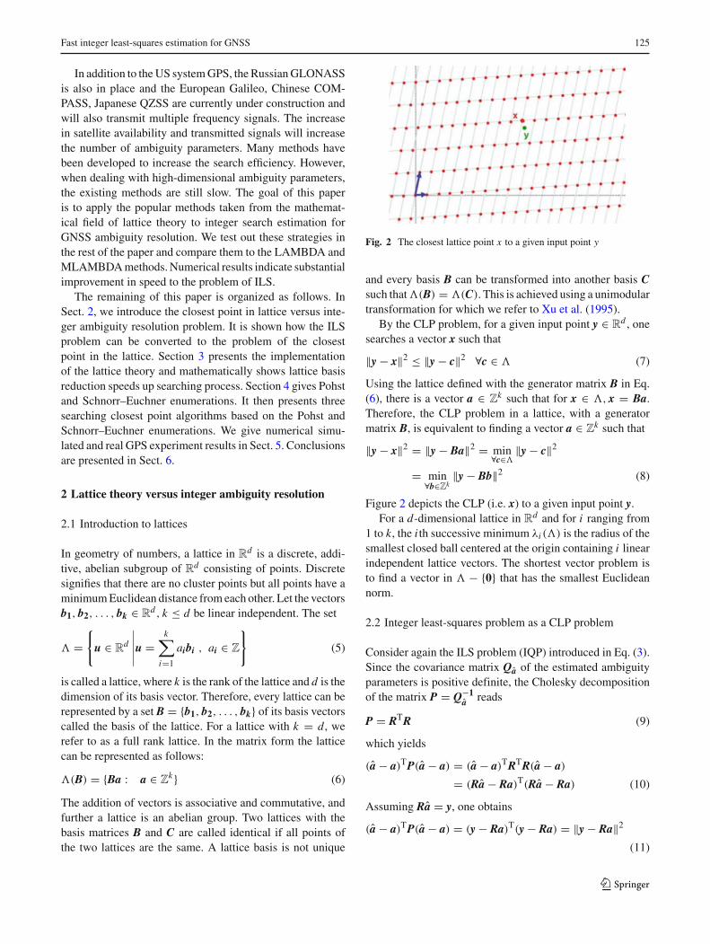
Fig. 2 The closest lattice point x to a given input point y
and every basis B can be transformed into another basis Csuch that �(B) = �(C). This is achieved using a unimodulartransformation for which we refer to Xu et al. (1995).
By the CLP problem, for a given input point y ∈ Rd , one
searches a vector x such that
‖y − x‖2 ≤ ‖y − c‖2 ∀c ∈ � (7)
Using the lattice defined with the generator matrix B in Eq.(6), there is a vector a ∈ Z
k such that for x ∈ �, x = Ba.Therefore, the CLP problem in a lattice, with a generatormatrix B, is equivalent to finding a vector a ∈ Z
k such that
‖y − x‖2 = ‖y − Ba‖2 = min∀c∈�‖y − c‖2
= min∀b∈Zk
‖y − Bb‖2 (8)
Figure 2 depicts the CLP (i.e. x) to a given input point y.For a d-dimensional lattice in R
d and for i ranging from1 to k, the i th successive minimum λi (�) is the radius of thesmallest closed ball centered at the origin containing i linearindependent lattice vectors. The shortest vector problem isto find a vector in � − {0} that has the smallest Euclideannorm.
2.2 Integer least-squares problem as a CLP problem
Consider again the ILS problem (IQP) introduced in Eq. (3).Since the covariance matrix Qa of the estimated ambiguityparameters is positive definite, the Cholesky decompositionof the matrix P = Q−1
a reads
P = RTR (9)
which yields
(a − a)TP(a − a) = (a − a)TRTR(a − a)
= (Ra − Ra)T(Ra − Ra) (10)
Assuming Ra = y, one obtains
(a − a)TP(a − a) = (y − Ra)T(y − Ra) = ‖y − Ra‖2
(11)
123
126 S. Jazaeri et al.
Therefore, ILS problem using Eq. (11) can be rewritten asfollows
a = min(a − a)TP(a − a) = min ‖y − Ra‖2 (12)
The preceding minimization problem is equivalent to theCLP problem of the lattice �(R) = {Ra : a ∈ Z
n}, with thebasis matrix R and the given point y. Therefore, ILS problemis in fact a CLP problem in lattice �(R).
3 Background on lattice basis reduction
3.1 Lattice basis reduction
Hermite (1850) published the first lattice reduction (LR)algorithm in an arbitrary dimension by trying to generalizeLagrange’s two-dimensional algorithm (Lagrange 1773). Inhis famous letters to Jacobi, Hermite described two reductionnotions (along with algorithms) in the language of quadraticforms: the first letter presented an algorithm to show the exis-tence of Hermite’s constant (which guarantees the existenceof short lattice vectors), while the second letter presenteda slightly different algorithm to further prove the existenceof lattice bases with bounded orthogonality defect (Nguyenand Stehlé 2009). Hermite’s algorithms can be viewed as theancestors of the Lenstra, Lenstra and Lovasz (LLL) algo-rithm.
In mathematics, the goal of lattice reduction is to trans-form a given lattice basis into another lattice basis of which itsvectors have the smallest possible length and they are close toorthogonal (for lattice-search problems, this was first notedby Coveyou and Macpherson 1967). There exists no per-fect lattice basis reduction algorithm because it depends onmany factors like runtime, dimension of the basis, the givenproblem to solve, and the expected quality of the solution.A perfect algorithm should be able to handle high-dimen-sional lattice and provide appropriate solutions in acceptabletime. Since the runtime plays an important role, a trade-off between the runtime and a good solution for a givenlattice problem is necessary. For example, Korkine–Zolota-reff (KZ) reduction is very strong, but expensive to com-pute. On the contrary, LLL reduction is fairly cheap, butan LLL-reduced basis is of much lower quality (Hanrotand Stehle 2007). The orthogonalization, size reduction, andvector swapping constitute the three fundamentals of thelattice basis reduction, which will be followed in the nextsubsections.
The covariance matrix of the ambiguities geometricallydefines a hyper-ellipsoid centered on the float ambiguities,related to the searching space. Within a short observationspan, there is a high correlation between ambiguities andthe search ellipsoid may be particularly elongated (Teunis-sen 1996). Therefore, the search process can be very time
consuming. In the GNSS literature, reduction stage is calleddecorrelation. To increase the searching speed for the CLPor integer ambiguities, one needs to decrease the correlationamong the original ambiguities. By a reparametrization ofthe ambiguities which is called decorrelation or reduction,the hyper ellipsoid is transformed to an almost spheroid andconsequently the searching process speeds up.
3.2 Orthogonalization
Consider the lattice basis B = (b1, b2, . . . , bn). The orthog-onalization process provides the Gram–Schmidt coefficientsgi j and the squared 2-norms of the orthogonalized latticebasis vectors b0
i , i.e. ‖b0i ‖2, with the help of QR decomposi-
tion using the Gram–Schmidt process in the shape of R:
R =
⎛⎜⎜⎜⎜⎜⎝
‖b01‖2 g2,1 · · · gn−1,1 gn,1
0 ‖b02‖2 g3,2 . . . gn,2
......
. . . . . ....
0 · · · 0 ‖b0n−1‖2 gn,n−1
0 0 · · · 0 ‖b0n‖2
⎞⎟⎟⎟⎟⎟⎠
(13)
QR decomposition and the Gram–Schmidt process aredescribed in Appendix. Basis orthogonalization is explainedin Algorithm 1.
Algorithm 1 Basis OrthogonalizationInput: Lattice basis B = (b1, b2, . . . , bn) ∈ R
n
Output: R1: Computing QR decomposition by means of Gram–Schmidt process2: for i = 1: n3: for j = i + 1: n4: ri, j = ri,j
ri,i
5: end for6: ri,i = r2
i,i
7: end for
3.3 Size reduction
A lattice basis B = (b1, b2, . . . , bn) is said to be size-reducedif its Gram–Schmidt orthogonalization coefficients gi j ’s allsatisfy |gi, j | ≤ 1
2 for all 1 ≤ j < i ≤ k. Size reduction wasintroduced by Lagrange (1773).
Any basis can be converted into a size reduced basis byAlgorithm 2.
Algorithm 2 Basis Size ReductionInput : Lattice basis B = (b1, b2, . . . , bn) ∈ R
n and the Gram–Schmidt coefficientsOutput : Size reduced basis B1: for i = 2 : n2: for j = i − 1 : n3: If |gi, j | > 1
24: bi = bi − round(gi, j )bj
5: gi, j = gi, j − round(gi, j )
6: for l = 1 : j − 1 gi,l = gi,l − round(gi, j )g j,l
7: End if8: end for9: end for
123
Fast integer least-squares estimation for GNSS 127
3.4 Vector swapping
To gain a better reduction, vector swapping is used whichis a unimodulary transformation operation. The order of bi
and then the dedicated orthogonalized versions b∗i will be
changed by swapping. Algorithm 2 demonstrates that thebasis vector bk can be size reduced using the Gram–Schmidtcoefficients by k−1 vectors, the vector bk−1 by k−2 vectors,and finally b2 by only one vector, i.e. b1. In this manner, thevector b1 itself is not size reduced. Consequently, the relativeshort vectors should be taken to the front and the long vec-tors to the end of the basis. Then, a long vector has a higherchance to get size reduced and the shortest vector cannot besize reduced at all.
It is useful to swap two vectors bi and bi+1 when the dedi-cated orthogonalized version b∗
i gets shorter. Swap conditionfor consecutive vectors bi and bi+1 is as follows (Lenstra et al.1982):
δ‖b∗i ‖2
2 ≤ ‖b∗i+1‖2
2 + g2i+1,i‖b∗
i ‖22
1
4< δ ≤ 1
i = 1, . . . , n − 1 (14)
LLL reduction proposed by Lenstra et al. (1982) who focusedon δ = 3
4 . Two types of reduction that are more frequentlyused in practice are Korkine–Zolotareff (KZ) reduction pro-posed by Korkine and Zolotareff (1873) and LLL reduction.A basis B = (b1, b2, . . . , bn) is LLL-reduced if it is size-reduced and if its Gram–Schmidt orthogonalization vectorssatisfy the (n − 1) conditions (14). This implies that thelengths of the b∗
i ’s cannot decrease too fast: intuitively, thevectors are not far from being orthogonal.
The LLL reduction is often used in situations where theKZ reduction would be too time consuming and terminates inpolynomial time according to the lattice dimension. One rea-son for their reputation is that their algorithms are recursive.The n-dimensional reduction problem can be recursivelyreduced to a n − 1-dimensional reduction problem whichis not feasible with Minkowski (1905) reduction. Findinggood reduced bases has proved invaluable in many fields ofcomputer science and mathematics (see for example, Cohen1995; Grotschel et al. 1993), particularly in cryptology (seefor instance, Nguyen and Stern 2001; Micciancio and Gold-wasser 2002). For the issue on numerical stability for latticebasis reduction algorithms the reader can consult for instance,Nguyen and Stehlé (2004, 2009) and Pujol and Stehle (2008).Recently improved lattice basis reduction algorithms arestudied in Bartkewitz (2009).
Definition 2 A Lattice is called δ-LLL-reduced when
1. it is size reduced2. δ‖b∗
i−1‖22 ≤ ‖b∗
i‖22 + g2
i,i−1‖b∗i−1‖2
2
i = 2, . . . , n 14 < δ ≤ 1
The LLL algorithm uses Gram–Schmidt process for theorthogonalization and the size reduction algorithm (Algo-rithm 2). Algorithm 3 shows the LLL algorithm.
Algorithm 3 LLL-Algorithm for basis reductionInput: Lattice basis B = (b1, b2, . . . , bn) and reduction parameter δ with 1
4 < δ < 1Output: δ-LLL-reduced basis B1: Using Gram–Schmidt process to compute coefficients gi, j
2: i = 23: while i ≤ n4: Using Algorithm 2 to size reduce the vector bi
5: If δ‖b∗i−1‖2
2 > ‖b∗i‖2
2 + g2i,i−1‖b∗
i−1‖22 then
6: Swap basis vectors bi and bi−1
7: Update Gram–Schmidt coefficients gl, j for l > j8: i = max(i − 1, 2)
9: else10: i = i + 111: end if12: end while
The decorrelation process is utilized to alter the integer ambi-guity resolution problem of Eq. (3) to a new one
a1 = min(a1 − a1)TP1(a1 − a1) (15)
by the so called G transformation such that
a1 = GTa P1 = GTPG (16)
where G is unimodular, i.e. |det(G)| = 1. When the opti-mal integer estimate of a1 in model (16) is found, the integerambiguity parameters a are calculated via a = (GT)−1a1.Since G is an integer matrix, G−1 and as a result a will remaininteger.
Several decorrelation techniques have been proposed inGNSS literature. We can point out the Gaussian decorrela-tion technique applied in LAMBDA, proposed by Teunissen(1995), inverse integer Cholesky decomposition proposed byXu (2001), LLL proposed by Hassibi and Boyed (1998) andGrafarend (2000), modified reduction algorithm proposed byChang et al. (2005), united ambiguity decorrelation proposedby Liu et al. (1999) and (inverse) paired Cholesky integertransformation proposed by Zhou (2010).
3.5 Why lattice reduction speeds up searching process?
We now mathematically show that the lattice reductionmethod reduces the numbers of candidates for searchingand consequently the searching process speeds up. Consideragain the ILS problem
‖a − a‖2P = (a − a)TP(a − a) = (Ra − Ra)T(Ra − Ra)
= ‖R(a − a)‖2 (17)
where R is the generator matrix of lattice �(R) = {Ra: a∈ Z
n}. Also, consider that the upper bound of ‖a − a‖2P is r2
i.e. ‖a − a‖2P ≤ r2. Applying a reduction algorithm such as
LLL algorithm to the row vectors of R−1 instead of R (thereason will become clear soon), we obtain R−1
r = UR−1, orequivalently
123
128 S. Jazaeri et al.
R = RrU (18)
Then
‖R(a−a)‖2 =‖RrU(a−a)‖2 =‖Rr(s−s)‖2 < r2 (19)
where s = Ua and s = Ua. Since (s − s) = R−1r Rr(s − s)
we have
(si − si) = r−1i Rr(s − s) (20)
Similarly
(ai − ai) = r−1i R(a − a) (21)
where si is the i th element of s, ai is the i th element of a, r−1i
denotes the i th row vector of R−1r and r−1
i denotes the i throw vector of R−1. Considering rr = Rr(s − s) and rr =R(a − a), where rr and rr are column vectors, and 〈.〉 denot-ing the inner product, one has
(si − si)2 =
(r−1
i Rr(s − s))2 =
(〈r−1
i .rr〉)2
(22)
(ai − ai)2 =
(r−1
i R(a − a))2 =
(〈r−1
i .rr〉)2
(23)
Applying the Cauchy–Shwarz inequality to the equationsyields
(si − si)2 =
(⟨r−1
i .rr
⟩)2 ≤∥∥∥r−1
i
∥∥∥2 ‖rr‖2
=∥∥∥r−1
i
∥∥∥2 ∥∥Rr(s − s)∥∥2 (24)
(ai − ai)2 =
(⟨r−1
i .rr
⟩)2 ≤∥∥∥r−1
i
∥∥∥2 ‖rr‖2
=∥∥∥r−1
i
∥∥∥2 ∥∥R(a − a)∥∥2 (25)
Equations (24) and (25) with Eq. (19) will convert to
(si − si)2 ≤
∥∥∥r−1i
∥∥∥2r2 (26)
(ai − ai)2 ≤
∥∥∥r−1i
∥∥∥2r2 (27)
Because U is a unimodular matrix we have det(U) = 1and hence det(R−1
r ) = det(R−1). According to Hadamard’sinequality we have
|det(R−1)| ≤n∏
i=1
∥∥∥r−1i
∥∥∥ (28)
For orthogonal vectors r−1i , equality is achieved and we have
(Mow 2003)
|det(R−1r )| =
n∏i=1
∥∥∥r−1i
∥∥∥ (29)
Equations (28) and (29) yield
n∏i=1
‖r−1i ‖ ≤
n∏i=1
∥∥∥r−1i
∥∥∥ (30)
Using Eqs. (26) and (27) we have
n∏i=1
∣∣(si − si)∣∣ ≤
n∏i=1
∥∥∥r−1i r∥∥∥ (31)
n∏i=1
∣∣(ai − ai)∣∣ ≤
n∏i=1
∥∥∥r−1i r∥∥∥ (32)
Using Eq. (30), the product∥∥∥r−1
1
∥∥∥∥∥∥r−1
2
∥∥∥ . . .∥∥r−1
n
∥∥ is smaller
than∥∥∥r−1
1
∥∥∥∥∥∥r−1
2
∥∥∥ . . .∥∥r−1
n
∥∥. Equations (31) and (32) indicate
that the numbers of candidates as a whole for searching in thereduced lattice will decrease and consequently the searchingprocess speeds up.
4 Closest point search algorithms
In this section, we start with a conceptual description of vari-ous lattice search algorithms. In this framework, we introducethe Pohst strategy, the Schnorr–Euchner refinement of the Po-hst strategy and three CLP search algorithms, i.e. Agrell, Eri-ksson, Vardy, Zeger (AEVZ), modification of Viterbo-Bou-tros (M-VB) and modification of Schnorr–Euchner (M-SE)that are basically applications of the studies by Fincke andPohst (1985)) and Schnorr and Euchner (1994).
Pohst (1981) proposed an efficient algorithm for enumer-ating all lattice points within a sphere with a certain radius.The search strategy used in the LAMBDA method, proposedby Teunissen (1993), is a variant of Pohst enumeration strat-egy. Pohst enumeration approach has been extensively usedin CLP search problems because of its efficiency.
Pohst closest point search algorithm is briefly outlined asfollows.
Consider the CLP problem in lattice �(R) defined inmodel (12). Let R0 be the squared radius of an n-dimen-sional sphere centered at y. Equation (12) gives
‖y − Ra‖2 ≤ R0 (33)
Due to the upper triangular form of R, the inequality impliesa set of conditions as
n∑j=i
⎛⎝y j −
m∑l= j
R j,lal
⎞⎠
2
≤ R0 i = 1, . . . , n (34)
Considering the above conditions in the order from i = ndown to 1, the set of admissible values of each variable ai isachieved using the values given for variables ai+1, . . . , an .More explicitly if the values of a j for i + 1 ≤ j ≤ n arefixed, the component ai , i = n − 1, n − 2, . . . , 1 can takevalues in the range of integers [Li , Ui ] where
123
Fast integer least-squares estimation for GNSS 129
Li = round
⎡⎢⎢⎣ 1
Ri,i
⎛⎝yi −
n∑j=i+1
Ri, j a j
−
√√√√√R0 −n∑
j=i+1
⎛⎝y j −
n∑l= j
R j,lal
⎞⎠
2⎞⎟⎟⎠⎤⎥⎥⎦ (35)
Ui = round
⎡⎣ 1
Ri,i
⎛⎝yi −
n∑j=i+1
Ri, j a j
+
√√√√√R0 −n∑
j=i+1
⎛⎝y j −
n∑l= j
R j,lal
⎞⎠
2⎞⎟⎟⎠⎤⎥⎥⎦ (36)
where round(.) denotes rounding to the closest integer. If
n∑j=i+1
⎛⎝y j −
n∑l= j
R j,lal
⎞⎠
2
> R0 (37)
there is no value of ai satisfying the inequalities (35) and(36). Therefore, the points corresponding to the fixed valuesai+1, . . . , an do not belong to the sphere with radius
√R0
centered at y. Pohst algorithm consists of spanning at eachlevel i the admissible interval [Li , Ui ], starting from leveli = n and climbing up to level i = n − 1, n − 2, . . . , 1. Ateach level, the interval [Li , Ui ] is determined by the valuesof the variables at lower levels corresponding to higher indi-ces. If the interval [L1, U1] is non-empty, all a ∈ [L1, U1]and fixed values of the variables at lower levels yield latticepoints in defined sphere with radius R0. The squared Euclid-ean distances between such points and y are
d2(y, Ra) =n∑
j=1
⎛⎝y j −
n∑l= j
R j,lal
⎞⎠
2
(38)
The Pohst algorithm provides the point a for which Euclideandistances defined in Eq. (38) is minimum. If, after spanningthe interval [Ln, Un], corresponding to an , no point in thesphere is found (empty sphere), the search fails. In this case,the search squared radius R0 must be increased and the searchis resumed with new squared radius. In Pohst method everyvariable ai takes values in the order Li , Li + 1, . . . , Ui ateach level. Schnorr–Euchner strategy is the variant of Po-hst strategy and the intervals at every level are spanned in azig-zag order, starting from the midpoint of the interval. Themidpoint of every interval at level i is as follows
Mi = round
⎛⎝ 1
Ri,i
⎛⎝yi −
n∑j=i+1
Ri, j a j
⎞⎠⎞⎠ (39)
In Schnorr–Euchner enumeration, every variable at level itakes values in the order Mi , Mi + 1, Mi − 1, Mi + 2, Mi −2, . . . , if
yi −n∑
j=i+1
Ri, j a j − Ri,i Mi ≥ 0 (40)
or, in the order Mi , Mi − 1, Mi + 1, Mi − 2, Mi + 2, . . . , if
yi −n∑
j=i+1
Ri, j a j − Ri,i Mi < 0 (41)
This enumeration strategy was firstly introduced by Schnorrand Euchner (1994). Teunissen (1995) explained that insteadof scanning the interval per ambiguity from left to right forintegers (Pohst strategy), one can search in an alternatingway around the conditional estimate in a zig-zag order. Thatstrategy is, however, different from Schnorr–Euchner strat-egy and selecting integer in the interval (per ambiguity) isnot based on the conditions (40) and (41). In Schnorr–Euch-ner strategy, R0 can be set to infinity (R0 = ∞) and there isno need to compute the search radius at first. In this way thesearch never fails and the first point found corresponds to theBabai point (Babai 1986; Agrell et al. 2002)
aBabaii = round
⎛⎝ 1
Ri,i
⎛⎝yi −
n∑j=i+1
Ri, j aBabaij
⎞⎠⎞⎠ (42)
An efficient closest point search algorithm, based on the Sch-norr–Euchner variant of the Pohst technique, is implementedby Agrell et al. (2002). We call this CLP search algorithmAEVZ, as an abbreviation for the names of the authors. Thisstrategy is shown to be considerably faster than other knownmethods, by means of a theoretical comparison with the Kan-nan algorithm (Kannan 1983) and an experimental compar-ison with the Pohst algorithm and its variants, such as theViterbo-Boutros decoder (Viterbo and Boutros 1999). Thealgorithm can be modified to solve a number of related searchproblems for lattices, which includes finding the shortest vec-tor, determining the kissing number, computing the Voronoi-relevant vectors, and finding a Korkine–Zolotareff reducedbasis (Agrell et al. 2002).
AEVZ is the variant of Pohst strategy and the intervals atevery level are spanned also based on Schnorr–Euchner enu-meration. The squared search radius is set to infinity. Basedon Schnorr–Euchner strategy, it is easy to see that the firstpoint found with R0 = ∞ corresponds to the Babai point.Therefore, the first lattice point generated will be the Babaipoint when the search process is starting from level i = n andreaching to level 1. After the Babai point is found, the R0 is setto the distance d2(y, RaBabai). In this manner the search neverfails. During the search process, the search sphere shrinkseach time when a new integer point is found. This is crucialto the efficiency of the search process. This method starts to
123
130 S. Jazaeri et al.
search a new candidate with returning to level 2 and take thenext integer at this level based on Schnorr–Euchner enumer-ation (Eqs. 40 and 41). If the new calculated squared searchradius is smaller than previous radius, the search processmoves to level 1, otherwise it proceeds with level 3 to takethe next integer value at this level. The search process willbe continued until a new candidate at level 1 will be found.Finally, when the search process fails to find a new integervalue at level n, i.e. its squared distance is larger than bestsquared distance found so far, the search process stops andthe latest integer point found is the optimal solution we lookfor.
Modification of the Schnorr–Euchner enumeration(M-SE) is similar to AEVZ CLP search algorithm. Thesquared radius search is, however, not considered infinitybut an input parameter (Damen et al. 2003). A too smallsquared radius may result in an empty sphere, whereas a toolarge one may result in too many points to be enumerated.A usual candidate for R0 is the covering radius, defined tobe the radius of the spheres centered at the lattice points thatcover the entire space in the most efficient way. The coveringradius can be computed by exhaustive search and the runningtime for exhaustive search becomes forbiddingly large. Thisproblem is called NP-hard (Guruswami et al. 2005). To cal-culate the initial squared radius R0, the reader is referred toTeunissen et al. (1997), Hassibi and Boyed (1998), Zhou andGiannakis (2005), and Hassibi and Vikalo (2005). The AEVZand M-SE methods are implemented in MATLAB and theircodes are provided in the supplementary electronic file.
The VB implementation (Viterbo and Boutros 1999) isa variant of Pohst strategy and contrary to the AEVZ CLPsearch algorithm, the squared search radius is set to R0. ButR0 is changed adaptively along the search. In this methodsearch strategy continue until it reaches level 1 and obtainthe first integer point. Then R0 is updated and the search isrestarted in the new sphere with smaller radius. The new pro-cess starts at level 1 to search through all other valid integersfrom the smallest to the largest. Then move up to level 2 toupdate the integer value to be the next nearest integer basedon Pohst enumeration. If it belongs to the authorized intervalat level 2, it moves down to level 1 to update the integer valueat this level; otherwise it moves up to level 3 to update theinteger value at this level and so on. Finally, when it fails tofind a new integer value at level n that satisfies the inequality(yn − Rn,nan)2 < R0, the search process stops. The latestinteger point found is the optimal solution we look for. Dur-ing the search process, the search sphere shrinks each timewhen a new integer point is found.
A drawback of this technique is that the VB algorithm mayre-span values of ai for some levels i, 1 ≤ i ≤ n, that havealready been spanned in the previous sphere. In modified-VB(M-VB) algorithm, once a lattice point is found, all the upperbounds of the intervals are updated without restarting. This is
the main advantage of this strategy over VB method. In otherwords, some values of ai that have already been examined,will not be reconsidered after reducing the sphere radius. Forfurther information, the reader is referred to Damen et al.(2003). The M-VB method is implemented in MATLAB andthe code is provided in the supplementary electronic file.
We point out that the AEVZ, M-VB and M-SE CLP searchalgorithms are the fastest algorithms currently available forfinding CLP, which can accordingly be used for ILS estima-tion.
5 Numerical results and discussion
To compare different search strategies for GNSS high-dimen-sional ambiguity resolution, in this section, we use manydifferent simulated data to compare the performance of threeinteger search methods presented in the previous section.This includes simulations such as those implemented inChang et al. (2005) applied to compare the LAMBDA andMLAMBDA, and simulations using algorithms presented byXu (2001). Further, we have also included results on a realGPS data set in which real ambiguity vector along with itscovariance matrix were used. We test out the searching speedof the methods and compare them to the LAMBDA andMLAMBDA. All presented results in this section are per-formed in MATLAB 7.6.0 on a PC, 2.8 GHz with 2.96 GBmemory running Windows XP professional.
We highlight that the goal is not to test the performanceof the LAMBDA and MLAMBDA. We hypothesize that theoriginal LAMBDA implemented in MATLAB by Delft Uni-versity of Technology is not likely optimized to allow for per-formance comparison in terms of computational efficiencybecause this available version is intended for educationalpurposes. We only compare searching speed of the methodspresented among each other and compare them to the cur-rent version of LAMBDA available in the website of DelftUniversity of Technology and the MLAMBDA provided byXiao-Wen Chang.
Simulations are performed for different cases. The realvector a was constructed as
a = 100 × randn(n, 1) (43)
where randn(n, 1) is a MATLAB built-in function to pro-duce a vector of n random entries having standard normaldistribution.
Similar to the simulations in Chang et al. (2005), to con-struct covariance matrix of real ambiguity parameters, weconsider seven cases. The first four cases are based on Qa =LTDL, where L is a unit lower triangular matrix with eachli j (for i > j) being a random number generated by randn,and D is generated in four different cases:
123
Fast integer least-squares estimation for GNSS 131
• Case 1: D = diag(di ), di = rand, where rand is a MAT-LAB built-in function to generate uniformly distributedrandom numbers in (0, 1).
• Case 2: D = diag(n−1, (n − 1)−1, . . . , 1)
• Case 3: D = diag(1, (2)−1, . . . , n−1)
• Case 4: D = diag(200, 200, 200, 0.1, 0.1, . . . , 0.1)
The other three cases are as follows:
• Case 5: Qa = UDUT , U is a random orthogonal matrixobtained by the QR factorization of a random matrixgenerated by randn(n, n), D = diag(di t), di = rand.
• Case 6: Qa = UDUT , U is generated in the same wayas in case 5, d1 = 2− n
4 , dn = 2n4 , other diagonal ele-
ments of D is randomly distributed between d1, dn, n isthe dimension of Qa. Thus the condition number of Qais 2
n2 .
• Case 7: Qa = ATA, A = randn(n, n).
Case 4 is motivated because the covariance matrix Qa inGPS usually has a large gap between the third conditionedstandard deviation and the forth one (Teunissen 1998a, Sect.8.3.3).
To fairly compare all search processes and to speed upsearching in all simulations, after applying the decorrelationprocess, we used the search algorithms to the transformedILS problem. All presented results are performed over 100independent runs. Numerical results just show the averagesearch time of the three presented algorithms (AEVZ, M-VB and M-SE), LAMBDA and MLAMDA. The compu-tation time for the decorrelation was not included. For theLAMBDA, MLAMBDA and the three lattice search algo-rithms, the Gaussian decorrelation method is used before thesearch process.
Because we used the same decorrelation method for allsearch algorithms, the total ILS estimation time will increaseby the same amount if we include the computation time forthe decorrelation. This indicates that only the computationtime of different search algorithms is of interest in the pres-ent contribution. Obviously, if we do not apply the decor-relation process and use the search process on the originalleast-squares problem, the search time for the presented algo-rithms, LAMBDA and MLAMBDA will all increase propor-tional to the computation search time presented for differentmethods when applying the decorrelation process. In eachrun the best optimal ILS is estimated and we search only forthe (first) best solution with LAMBDA and MLAMBDA.The average integer searching time (excluding the reductiontime) for all simulated data and for dimensions of 40 and 45are given below.
For weak models in which the success rate is low, thedecorrelation and search time will generally be longer. Tohave strong models, in all simulations, the success rate is
considered to be 99.999%. To reach exactly this high successrate, the simulated covariance matrices in some cases willslightly be scaled as Qa = σ Qa. A simple measure to inferthe float ambiguity precision is the ambiguity dilution of pre-cision (ADOP) defined in Teunissen (1997). We applied thesuccess rate defined in Teunissen (1998b), which is a func-tion of ADOP. Average searching time in seconds for allsimulation cases are presented in Table 1.
We also constructed the real vector a using the MATLABbuilt-in function in the statistics toolbox (mvnrnd.m), whichallows to generate the ambiguities for a given covariancematrix. Tables 2 and 3 outline the results of all simulationcases 1–7 for dimensions n = 40 and n = 45, respectively.
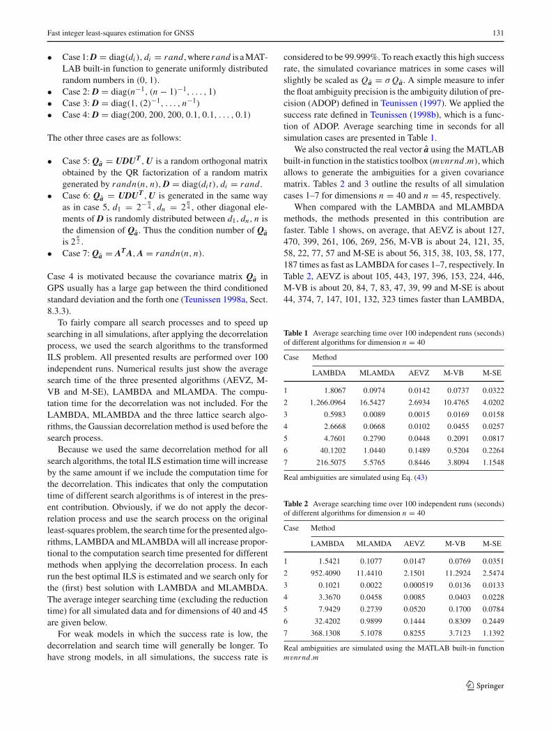
When compared with the LAMBDA and MLAMBDAmethods, the methods presented in this contribution arefaster. Table 1 shows, on average, that AEVZ is about 127,470, 399, 261, 106, 269, 256, M-VB is about 24, 121, 35,58, 22, 77, 57 and M-SE is about 56, 315, 38, 103, 58, 177,187 times as fast as LAMBDA for cases 1–7, respectively. InTable 2, AEVZ is about 105, 443, 197, 396, 153, 224, 446,M-VB is about 20, 84, 7, 83, 47, 39, 99 and M-SE is about44, 374, 7, 147, 101, 132, 323 times faster than LAMBDA,
Table 1 Average searching time over 100 independent runs (seconds)of different algorithms for dimension n = 40
Case Method
LAMBDA MLAMDA AEVZ M-VB M-SE
1 1.8067 0.0974 0.0142 0.0737 0.0322
2 1,266.0964 16.5427 2.6934 10.4765 4.0202
3 0.5983 0.0089 0.0015 0.0169 0.0158
4 2.6668 0.0668 0.0102 0.0455 0.0257
5 4.7601 0.2790 0.0448 0.2091 0.0817
6 40.1202 1.0440 0.1489 0.5204 0.2264
7 216.5075 5.5765 0.8446 3.8094 1.1548
Real ambiguities are simulated using Eq. (43)
Table 2 Average searching time over 100 independent runs (seconds)of different algorithms for dimension n = 40
Case Method
LAMBDA MLAMDA AEVZ M-VB M-SE
1 1.5421 0.1077 0.0147 0.0769 0.0351
2 952.4090 11.4410 2.1501 11.2924 2.5474
3 0.1021 0.0022 0.000519 0.0136 0.0133
4 3.3670 0.0458 0.0085 0.0403 0.0228
5 7.9429 0.2739 0.0520 0.1700 0.0784
6 32.4202 0.9899 0.1444 0.8309 0.2449
7 368.1308 5.1078 0.8255 3.7123 1.1392
Real ambiguities are simulated using the MATLAB built-in functionmvnrnd.m
123
132 S. Jazaeri et al.
Table 3 Average searching time over 100 independent runs (seconds)of different algorithms for dimension n = 45
Case Method
LAMBDA MLAMDA AEVZ M-VB M-SE
1 4.7110 0.3246 0.0508 0.2482 0.0892
2 6,279.4891 83.428 13.2846 81.3527 27.2622
3 0.4278 0.0011 0.0006389 0.0187 0.0186
4 9.3553 0.1196 0.0231 0.0864 0.0474
5 21.6018 1.0358 0.1859 0.5323 0.2590
6 269.1465 4.5191 0.8125 3.3407 0.9809
7 2,117.5926 30.5525 6.1057 24.7601 7.6046
Real ambiguities are simulated using the MATLAB built-in functionmvnrnd.m
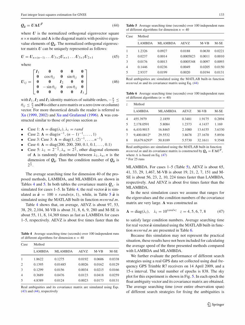
respectively. In Table 3, AEVZ is about 92, 472, 669, 404,116, 331, 347, M-VB is about 19, 77, 23, 108, 40, 80, 85 andM-SE is about 53, 230, 23, 197, 83, 274, 278 times as fast asLAMBDA, respectively. AEVZ is about 7, 6, 6, 7, 6, 7, and7 times in Table 1, 7, 5, 4, 5, 5, 7, and 6 times in Table 2 and6, 6, 2, 5, 6, 6, and 5 times in Table 3 as fast as MLAMBDAfor cases 1–7, respectively.
When AEVZ is compared to the M-VB and M-SE, itappears to be the fastest method. The results of the aver-age searching time (in seconds) are provided for the AEVZmethod in Fig. 3, for n = 10, 11, . . . , 50. Also Fig. 4 showsthe average number of candidates searched in each case.
Another simulation algorithm was proposed by Xu (2001).Let Qa be decomposed as follows:
Fig. 3 Average searching time (seconds) in logarithmic scale for the AEVZ method over 100 independent runs for cases 1–7
Fig. 4 Average number of candidates for the AEVZ method searched over 100 independent runs for cases 1–7
123
Fast integer least-squares estimation for GNSS 133
Qa = U�UT (44)
where U is the normalized orthogonal eigenvector squaren×n matrix and � is the diagonal matrix with positive eigen-value elements of Qa. The normalized orthogonal eigenvec-tor matrix U can be uniquely represented as follows:
U = Un×(n−1) . . . U3×2Un×1 . . . U3×1U2×1 (45)
where
Ui j =
⎡⎢⎢⎢⎢⎣
I1 0 0 0 00 cos θi j 0 sin θi j 00 0 I2 0 00 − sin θi j 0 cos θi j 00 0 0 0 I3
⎤⎥⎥⎥⎥⎦ (46)
with I1, I2 and I3 identity matrices of suitable orders, −π2 ≤
θi j ≤ π2 and 0 is either a zero matrix or a zero (row or column)
vector. For more theoretical details the reader is referred toXu (1999, 2002) and Xu and Grafarend (1996). � was con-structed similar to those of previous section as
of � is randomly distributed between λ1, λn, n is thedimension of Qa. Thus the condition number of Qa is2
n2 .
The average searching time for dimension 40 of the pro-posed methods, LAMBDA, and MLAMBDA are shown inTables 4 and 5. In both tables the covariance matrix Qa ‘ issimulated for cases 1–5. In Table 4, the real vector a is sim-ulated as a = 100 × randn(n, 1), while, in Table 5 a issimulated using the MATLAB built-in function mvnrnd.m.
Table 4 shows that, on average, AEVZ is about 97, 53,38, 29, 2,104, M-VB is about 31, 8, 6, 9, 280 and M-SE isabout 55, 11, 8, 14,369 times as fast as LAMBDA for cases1–5, respectively. AEVZ is about five times faster than the
Table 4 Average searching time (seconds) over 100 independent runsof different algorithms for dimension n = 40
Case Method
LAMBDA MLAMBDA AEVZ M-VB M-SE
1 1.8622 0.1275 0.0192 0.0606 0.0338
2 0.1395 0.01485 0.0026 0.0162 0.0129
3 0.1299 0.0156 0.0034 0.0215 0.0166
4 0.3689 0.0476 0.0123 0.0418 0.0259
5 4.8389 0.0124 0.0023 0.0173 0.0131
Real ambiguities and its covariance matrix are simulated using Eqs.(43) and (44), respectively
Table 5 Average searching time (seconds) over 100 independent runsof different algorithms for dimension n = 40
Case Method
LAMBDA MLAMBDA AEVZ M-VB M-SE
1 1.2326 0.0927 0.0188 0.0630 0.0221
2 0.0237 0.0014 0.0005823 0.0011 0.0010
3 0.0176 0.0013 0.0005348 0.0097 0.0093
4 0.1446 0.0236 0.0049 0.0205 0.0150
5 2.9337 0.0199 0.0020 0.0194 0.0131
Real ambiguities are simulated using the MATLAB built-in functionmvnrnd.m and its covariance matrix using Eq. (44)
Table 6 Average searching time (seconds) over 100 independent runsof different algorithms (n = 40)
z Method
LAMBDA MLAMBDA AEVZ M-VB M-SE
4 455.3979 2.1859 0.3481 1.9175 0.2894
5 2,178.0591 5.8084 1.2373 4.1437 1.169
6 6,410.9015 16.8465 2.1080 13.6155 3.6330
7 9,400.0812a 29.5532 3.8678 27.1670 5.8936
8 10,679.6293a 50.8189 5.5730 32.1611 9.3548
Real ambiguities are simulated using the MATLAB built-in functionmvnrnd.m and its covariance matrix is constructed by Qa = U�UT ,where � is based on Eq. (47)a For 25 runs
MLAMBDA. For cases 1–5 (Table 5), AEVZ is about 65,41, 33, 29, 1,467, M-VB is about 19, 21, 2, 7, 151 and M-SE is about 56, 23, 2, 10, 224 times faster than LAMBDA,respectively. And AEVZ is about five times faster than theMLAMBDA.
In the next simulation cases we assume that ranges forthe eigenvalues and the condition numbers of the covariancematrix are very large. � was constructed as
to satisfy large condition numbers. Average searching timefor real vector a simulated using the MATLAB built-in func-tion mvnrnd.m are presented in Table 6.
Because this simulation may not represent the practicalsituation, these results have not been included for calculatingthe average speed of the three presented methods comparedwith LAMBDA and MLAMBDA.
We further evaluate the performance of different searchstrategies using a real GPS data set collected using dual fre-quency GPS Trimble R7 receivers on 14 April 2009, and a15-s interval. The total number of epochs is 838. The skyplot for this experiment is shown in Fig. 5. In each epoch thefloat ambiguity vector and its covariance matrix are obtained.The average searching time (over entire observation span)of different search strategies for fixing the ambiguities is
123
134 S. Jazaeri et al.
Fig. 5 The sky plot of all observed satellites in view above 13 degreeelevation angle for entire time span of 5:25:15 till 8:54:45 on 14 April2009
Table 7 Average searching time (seconds) of different algorithms
Method
LAMBDA MLAMBDA AEVZ M-VB M-SE
12.0195 0.2357 0.0338 0.1844 0.0534
presented in Table 7. In this case we do not apply the dec-orrelation process and use the search process on the originalleast-squares problem. Similar results to those presented forthe simulated cases are obtained. Among them, it is clearthat the AEVZ is the fastest method to the solution of theILS estimation problem.
The proposed methods speed up searching CLP in latticesand give the optimal integer solution. The results in generalshow that these methods are faster than the LAMBDA andMLAMBDA methods.
6 Summary and conclusions
There exist several methods for ILS estimation. In caseswhere tens of integer ambiguities are involved, the exist-ing methods are still slow. In this contribution, we investi-gated the ILS estimation problem, which was shown to be thesame as the CLP problem in lattice theory. The mathemat-ical formulations of three efficient CLP search algorithms,i.e. AEVZ, M-SE and M-VB were presented.
AEVZ and M-SE algorithms are inspired by Schnorr–Eu-chner enumeration strategy and M-VB is inspired by Pohst
enumeration strategy. M-VB is more efficient than the VBsearching algorithm. M-SE is similar to AEVZ search algo-rithm but the squared radius search is not infinity but an inputparameter. In AEVZ search algorithm, search radius is set toinfinity and therefore the search never fails. These algorithmscan all be utilized to solve any IQP problem, including theleast-squares integer estimation of ambiguity parameters.
We discussed the mathematical background and pre-sented their implementations. We then tested the perfor-mance of the algorithms using different simulated and realGPS data. AEVZ, M-SE and M-VB methods when com-pared to the available version of LAMBDA and MLAMBDAwere proved to be faster on all simulated and real data. Thenumerical examples show that, on average, AEVZ is about320 times, M-VB is about 50 times and M-SE is about 120times faster than LAMBDA for dimension 40. These num-bers change to about 350, 60 and 160 times for dimension 45,which shows its efficiency at higher dimensions. The AEVZwas shown to be about 5 times faster than MLAMBDA.
Research into the performance of the presented algorithmsfor a constrained ILS estimation is ongoing and will be thesubject of future publications.
Acknowledgments The authors gratefully acknowledge Xiao-WenChang for providing us with the MILES package. Thanks also go toPeiliang Xu for introducing a few references and to Peter Teunissen forhis valuable comments on an earlier version of this paper. The authorswould also like to acknowledge the valuable comments of the editor,Pascal Willis, the editor-in-chief, Roland Klees, and three anonymousreviewers, which significantly improved the presentation and quality ofthis paper.
Appendix
Proposition 1 (Q R decomposition) Let A ∈ Rd×k and be
non-singular, then the QR decomposition A = QR is unique,where Q is unitary and R is an upper triangular matrix withpositive diagonal elements Golub and Loan (1996).
A = (a1, a2, . . . , ak)
= QR = (q1, q2, . . . , qk)
⎡⎢⎢⎢⎣
r1,1 r1,2 · · · r1,k
0 r2,2 · · · r2,k...
.... . .
...
0 0 · · · rk,k
⎤⎥⎥⎥⎦ (1)
Proposition 2 (Gram–Schmidt orthogonalization) The ort-hogonal basis b0
i of the basis vectors bi determined by thefollowing iterated process is called the Gram–Schmidt pro-cess:
b01 = b1 (2)
b0i = bi −
i−1∑j=1
gi, j b0j (3)
123
Fast integer least-squares estimation for GNSS 135
where
gi, j =
⎧⎪⎪⎪⎨⎪⎪⎪⎩
⟨bi,b0
j
⟩⟨b0
j ,b0j
⟩ i > j
1 i = j0 else
(4)
The Gram–Schmidt process gives the QR decomposition ofa basis B = (b1b2 . . . bk) such that
Q = (q1, q2, . . . , qn) =(
b01
‖b01‖2
,b0
2
‖b02‖2
, . . . ,b0
k
‖b0k‖2
)(5)
and
R =
⎡⎢⎢⎢⎣
r1,1 r1,2 · · · r1,k
0 r2,2 · · · r2,k...
.... . .
...
0 0 · · · rk,k
⎤⎥⎥⎥⎦
=
⎡⎢⎢⎢⎣
‖b01‖2 0 · · · 00 ‖b0
2‖2 · · · 0...
.... . .
...
0 0 · · · ‖b0k‖2
⎤⎥⎥⎥⎦× R∗ (6)
where
R∗ =
⎡⎢⎢⎢⎢⎢⎣
1 g2,1 · · · gk−1,1 gk,1
0 1 g3,2 · · · gk,2...
.... . .
......
0 · · · 0 1 gk,k−1
0 0 · · · 0 1
⎤⎥⎥⎥⎥⎥⎦
(7)
The Gram–Schmidt orthogonalization algorithm and theinverse integer Cholesky decorrelation method are imple-mented in MATLAB and their codes are provided in the sup-plementary electronic file.
References
Agrell E, Eriksson T, Vardy A, Zeger K (2002) Closest point search inlattices. IEEE Trans Inf Theory 48:2201–2214
Babai L (1986) On Lováasz’ lattice reduction and the nearest latticepoint problem. Combinatorica 6:1–13
Bartkewitz T (2009) Improved lattice basis reduction algorithms andtheir efficient implementation on parallel systems. Diploma the-sis, Ruhr University, Germany
Buist PJ (2007) The baseline constrained LAMBDA method for sin-gle epoch, single frequency attitude determination applications.In: Proceedings of ION GPS, p 12
Chang X, Yang X, Zhou T (2005) MLAMBDA: a modified LAMBDAalgorithm for integer least-squares estimation. J Geod 79:552–565
Chen D (1994) Development of a fast ambiguity search filtering(FASF) method for GPS carrier phase ambiguity resolution. UCGEReports 20071, PhD dissertation
Chen D, Lachapelle G (1995) A comparison of the FASF and least-squares search algorithms for on-the-fly ambiguity resolution, nav-igation. J Inst Navig 42(2):371–390
Cohen CE (1996) Attitude determination. In: Parkinson BW, Spilker JJ(eds) Global positioning system: theory and applications II. AIAA,Washington, pp 519–538
Cohen H (1995) A course in computational algebraic number theory.Springer, Berlin
Coveyou RR, Macpherson RD (1967) Fourier analysis of uniform ran-dom number generations. J ACM 14(1):100–119
Damen MO, El Gamal H, Caire G (2003) On maximum-likelihooddetection and the search for the closest lattice point. IEEE TransInf Theory 49(10):2389–2402
Fincke U, Pohst M (1985) Improved methods for calculating vectorsof short length in a lattice, including a complexity analysis. MathComput 44(170):463–471
Frei E, Beutler G (1990) Rapid static positioning based on the fast ambi-guity resolution approach “FARA”: theory and first results. Manu-scr Geod 15:325–356
Golub GH, Van Loan CF (1996) Matrix computations, 3rd edn. TheJohns Hopkins University Press, Baltimore
Grotschel M, Lovász L, Schrijver A (1993) Geometric algorithms andcombinatorial optimization. Springer, Berlin
Guruswami V, Micciancio D, Regev O (2005) The complexity of thecovering radius problem. Comput Complex 14:90–121
Hanrot G, Stehle D (2007) Improved analysis of Kannan’s shortestlattice vector algorithm. In: Advances in cryptology—crypto 2007,proceedings. A. Menezes, vol 4622, pp 170–186
Hassibi A, Boyed S (1998) Integer parameter estimation in linear mod-els with applications to GPS. IEEE Trans Signal Proc 46:2938–2952
Hassibi B, Vikalo H (2005) On the sphere-decoding algorithm I.expected complexity. IEEE Trans Signal Proc 53:2806–2818
Hermite C (1850) Extraits de lettres de M. Hermite à M. Jacobi surdiff′erents objets de la th′eorie des nombres. J Reine Angew Math40:279–290
Kannan R (1983) Improved algorithms for integer programming andrelated lattice problems. Paper presented at the conference pro-ceedings of the annual ACM symposium on theory of computing,pp 193–206
Kannan R (1987) Algorithmic geometry of numbers. Annu Rev Com-put Sci 16:231–267
Kim D, Langley RB (2000) A search space optimization techniquefor improving ambiguity resolution and computational efficiency.Earth Planets Space 52(10):807–812
Korkine A, Zolotareff G (1873) Sur les formes quadratiques. Math Ann-alen 6(3):366–389 (in French)
Lagrange JL (1773) Recherches d’arithmetique. Nouveaux Memoiresde l’Academie de Berlin
Langley RB, Beutler G, Delikaraoglou D, Nickerson B, Santerre R, Va-nicek P, Well DE (1984) Studies in the application of the GPS todifferential positioning. Technical Report No. 108, University ofNew Brunswick, Canada
Lenstra AK, Lenstra HW, Lovász L (1982) Factoring polynomials withrational coefficients. Math Ann 261:513–534
Liu LT, Hsu HT, Zhu YZ, Ou JK (1999) A new approach to GPS ambi-guity decorrelation. J Geod 73:478–490
Micciancio D, Goldwasser S (2002) Complexity of lattice problems: acryptographic perspective. Kluwer international series in engineer-ing and computer science, vol 671. Kluwer Academic Publishers,Boston
Minkowski H (1905) Diskontinuitätsbereich für arithmetische Äquival-enz. J Rreine Angew Math 129:220–274 (in German)
Mow WH (2003) Universal lattice decoding: principle and recentadvances. Wirel Commun Mobile Comput 3(5):553–569
Nguyen PQ, Stehlé D (2004) Low-dimensional lattice basis reductionrevisited (extended abstract). In: Proceedings of the 6th interna-
123
136 S. Jazaeri et al.
tional algorithmic number theory symposium (ANTS-VI), lecturenotes in computer science, vol 3076. Springer, Berlin, pp 338–357
Nguyen PQ, Stehlé D (2009) An LLL algorithm with quadratic com-plexity. SIAM J Comput 39(3):874–903
Nguyen PQ, Stern J (2001) The two faces of lattices in cryptology. In:Proceedings of CALC ’01, lecture notes in computer science, vol2146. Springer, Berlin, pp 146–180
Pohst M (1981) On the computation of lattice vector of minimal length,successive minima and reduced bases with applications. ACMSIGSAM Bull 15:37–44
Pujol X, Stehle D (2008) Rigorous and efficient short lattice vectorsenumeration. In: Advances in cryptology—Asiacrypt 2008 J Pie-przyk, vol 5350, pp 390–405
Schnorr CP, Euchner M (1994) Lattice basis reduction: improved prac-tical algorithms and solving subset sum problems. Math Program66:181–199
Steinfeld R, Pieprzyk J, Wang H (2007) Lattice-based thresholdchangeability for standard Shamir secret-sharing schemes. IEEETrans Inf Theory 53:2542–2559
Teunissen PJG (1993) Least-squares estimation of the integer GPSambiguities. Invited lecture, section IV theory and methodology,IAG general meeting, Beijing, China. Also in Delft Geodetic Com-puting Centre LGR series, No. 6, p 16
Teunissen PJG (1994) A new method for fast carrier phase ambiguityestimation. In: Proceedings of the IEEE PLANS’94, Las Vegas,NV, 11–15 April 1994, pp 562–573
Teunissen PJG (1995) The least-squares ambiguity decorrelationadjustment: a method for fast GPS ambiguity estimation. J Geod70:65–82
Teunissen PJG (1996) An analytical study of ambiguity decorrelationusing dual frequency code and carrier phase. J Geod 70:515–528
Teunissen PJG (1997) A canonical theory for short GPS baselines, partsI–IV. J Geod 71:320–336, 389–401, 486–501, 513–525
Teunissen PJG (1998b) Success probability of integer GPS ambiguityrounding and bootstrapping. J Geod 72:606–612
Teunissen PJG, De Jonge PJ, Tiberius CC (1997) The least-squaresambiguity decorrelation adjustment: its performance on short GPSbaselines and short observation spans. J Geod 71:589–602
Viterbo E, Boutros J (1999) A universal lattice code decoder for fadingchannels. IEEE Trans Inf Theory 45(5):1639–1642
Wei Z (1986) Positioning with NAVSTAR, the global positioning sys-tem. Report No. 370, Department of Geodetic Science and Sur-veying, The Ohio State University, Columbus, OH
Xu PL (1998) Mixed integer observation models and integer program-ming in geodesy. J Geod Soc Jpn 44:169–187
Xu PL (1999) Spectral theory of constrained second-rank symmetricrandom tensors. Geophys J Int 138(1):1–24
Xu PL (2001) Random simulation and GPS decorrelation. J Geod75:408–423
Xu PL (2002) Isotropic probabilistic models for directions, planes andreferential systems. Proc R Soc Lond Ser A 458(2024):2017–2038
Xu PL (2006) Voronoi cells, probabilistic bounds and hypothesis testingin mixed integer linear models. IEEE Trans Inf Theory 52:3122–3138
Xu PL, Grafarend E (1996) Statistics and geometry of the eigenspec-tra of three-dimensional second-rank symmetric random tensors.Geophys J Int 127(3):744–756
Xu PL, Cannon E, Lachapelle G (1995) Mixed integer programming forthe resolution of GPS carrier phase ambiguities. Paper presentedat IUGG95 assembly, Boulder, 2–14 July