Fast Inversion of Logging-While-Drilling (LWD) Resistivity Measurements David Pardo 1 Carlos Torres-Verd´ ın 2 1 University of the Basque Country (UPV/EHU) and Ikerbasque, Bilbao, Spain. 2 The University of Texas at Austin, USA 17 Oct. 2013 BCAM Workshop on Computational Mathematics, Bilbao, Spain 1
Transcript
Fast Inversion of Logging-While-Drilling(LWD) Resistivity Measurements
David Pardo 1 Carlos Torres-Verdın 2
1University of the Basque Country (UPV/EHU) andIkerbasque, Bilbao, Spain.
2The University of Texas at Austin, USA
17 Oct. 2013BCAM Workshop on
Computational Mathematics, Bilbao, Spain
1
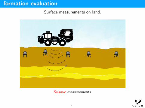
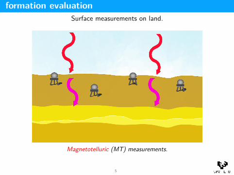
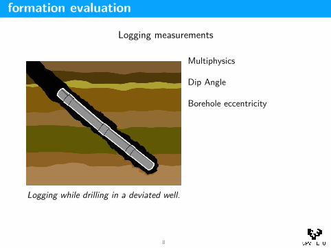
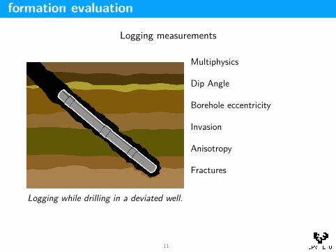
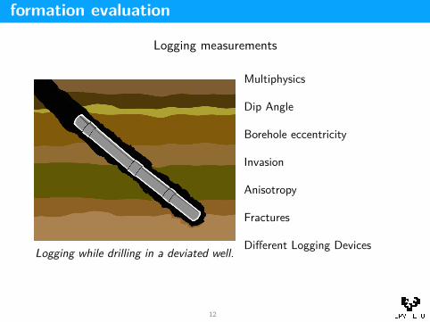
formation evaluationSurface measurements on the sea.
Marine seismic measurements.
2
formation evaluationSurface measurements on the sea.
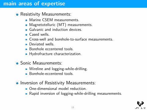
Resistivity Measurements:Marine CSEM measurements.Magnetotelluric (MT) measurements.Galvanic and induction devices.Cased wells.Cross-well and borehole-to-surface measurements.Deviated wells.Borehole eccentered tools.Hydrofracture characterization.
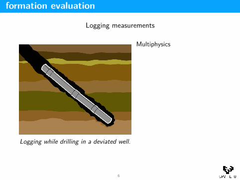
Sonic Measurements:Wireline and logging-while-drilling.Borehole-eccentered tools.
Inversion of Resistivity Measurements:One-dimensional model reduction.Rapid inversion of logging-while-drilling measurements.
13
main areas of expertise
Resistivity Measurements:Marine CSEM measurements.Magnetotelluric (MT) measurements.Galvanic and induction devices.Cased wells.Cross-well and borehole-to-surface measurements.Deviated wells.Borehole eccentered tools.Hydrofracture characterization.
Sonic Measurements:Wireline and logging-while-drilling.Borehole-eccentered tools.
Inversion of Resistivity Measurements:One-dimensional model reduction.Rapid inversion of logging-while-drilling measurements.
14
inversion of LWD measurements
Motivation and objectives.
Assumptions.
Forward Problem.
Inverse Problem.
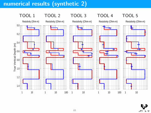
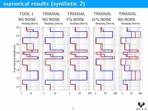
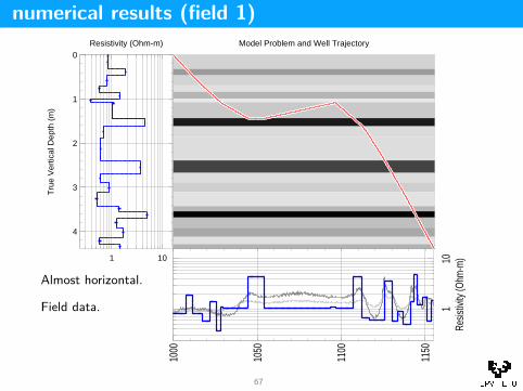
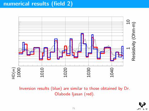
Numerical Results.
Conclusions.
15
motivation and objectives
Goal: Inversion of LWD resistivity measurements.
We want the inversion algorithm to be:
Efficient. Inversion in real time using 1D model reduction.
Flexible. It should enable the dynamic selection of a subset ofmeasurement and/or unknowns during inversion.
Robust. It should always converge to physically meaningfulsolutions.
Reliable. It should provide error bars.
Useful. It should work for any commercial LWD instrumentwith actual field measurements.
16
motivation and objectives
Goal: Inversion of LWD resistivity measurements.We want the inversion algorithm to be:
Efficient. Inversion in real time using 1D model reduction.
Flexible. It should enable the dynamic selection of a subset ofmeasurement and/or unknowns during inversion.
Robust. It should always converge to physically meaningfulsolutions.
Reliable. It should provide error bars.
Useful. It should work for any commercial LWD instrumentwith actual field measurements.
17
motivation and objectives
Goal: Inversion of LWD resistivity measurements.We want the inversion algorithm to be:
Efficient. Inversion in real time using 1D model reduction.
Flexible. It should enable the dynamic selection of a subset ofmeasurement and/or unknowns during inversion.
Robust. It should always converge to physically meaningfulsolutions.
Reliable. It should provide error bars.
Useful. It should work for any commercial LWD instrumentwith actual field measurements.
18
motivation and objectives
Goal: Inversion of LWD resistivity measurements.We want the inversion algorithm to be:
Efficient. Inversion in real time using 1D model reduction.
Flexible. It should enable the dynamic selection of a subset ofmeasurement and/or unknowns during inversion.
Robust. It should always converge to physically meaningfulsolutions.
Reliable. It should provide error bars.
Useful. It should work for any commercial LWD instrumentwith actual field measurements.
19
motivation and objectives
Goal: Inversion of LWD resistivity measurements.We want the inversion algorithm to be:
Efficient. Inversion in real time using 1D model reduction.
Flexible. It should enable the dynamic selection of a subset ofmeasurement and/or unknowns during inversion.
Robust. It should always converge to physically meaningfulsolutions.
Reliable. It should provide error bars.
Useful. It should work for any commercial LWD instrumentwith actual field measurements.
20
motivation and objectives
Goal: Inversion of LWD resistivity measurements.We want the inversion algorithm to be:
Efficient. Inversion in real time using 1D model reduction.
Flexible. It should enable the dynamic selection of a subset ofmeasurement and/or unknowns during inversion.
Robust. It should always converge to physically meaningfulsolutions.
Reliable. It should provide error bars.
Useful. It should work for any commercial LWD instrumentwith actual field measurements.
21
assumptions
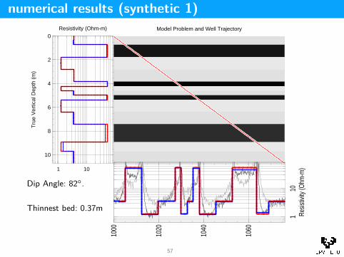
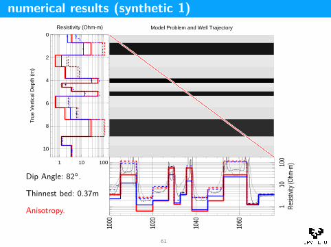
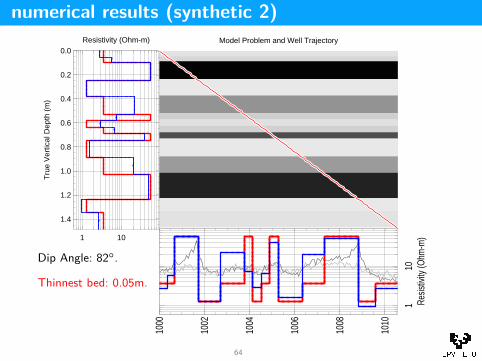
We assume a planarly TI layered media with piecewiseconstant resistivities.We assume no borehole effects and no mandrel effects.
1000 1050 1100 1150
0
1
2
3
4
Model Problem and Well Trajectory
Horizontal Depth (m)
True
Ver
tical
Dep
th (m
)
1000 1050 1100 1150
0
1
2
3
4
Model Problem and Well Trajectory
Horizontal Depth (m)
Tru
e V
ertic
al D
epth
(m
)
1000 1050 1100 1150
0
1
2
3
4
Model Problem and Well Trajectory
Horizontal Depth (m)
Tru
e V
ertic
al D
epth
(m
)
1000 1050 1100 1150
0
1
2
3
4
Model Problem and Well Trajectory
Horizontal Depth (m)
True
Ver
tical
Dep
th (m
)
We know the bedboundaries a priori.
We know the dip andazimuthal angles ofintersection a priori.
22
forward problem
Magnetic field H produced by a magnetic dipole is obtained usinga semi-analytical solution for a 1D planarly layered TI media(Kong, 1972).
A) Hankel transform in the horizontal plane.
B) Analytical solution of the resulting ordinary differentialequation in the vertical direction.
C) Numerical inverse Hankel transform (integration).
Result: Magnetic field H.
23
forward problem
Magnetic field H produced by a magnetic dipole is obtained usinga semi-analytical solution for a 1D planarly layered TI media(Kong, 1972).
A) Hankel transform in the horizontal plane.
B) Analytical solution of the resulting ordinary differentialequation in the vertical direction.
C) Numerical inverse Hankel transform (integration).
Result: Magnetic field H.
24
forward problem
Magnetic field H produced by a magnetic dipole is obtained usinga semi-analytical solution for a 1D planarly layered TI media(Kong, 1972).
A) Hankel transform in the horizontal plane.
B) Analytical solution of the resulting ordinary differentialequation in the vertical direction.
C) Numerical inverse Hankel transform (integration).
Result: Magnetic field H.
25
forward problem
Magnetic field H produced by a magnetic dipole is obtained usinga semi-analytical solution for a 1D planarly layered TI media(Kong, 1972).
A) Hankel transform in the horizontal plane.
B) Analytical solution of the resulting ordinary differentialequation in the vertical direction.
C) Numerical inverse Hankel transform (integration).
Result: Magnetic field H.
26
forward problem
Magnetic field H produced by a magnetic dipole is obtained usinga semi-analytical solution for a 1D planarly layered TI media(Kong, 1972).
A) Hankel transform in the horizontal plane.
B) Analytical solution of the resulting ordinary differentialequation in the vertical direction.
C) Numerical inverse Hankel transform (integration).
Result: Magnetic field H.
27
forward problem
CASE I: Triaxial Induction.
H =
Hxx Hxy HxzHyx Hyy HyzHzx Hzy Hzz
.
28
forward problem
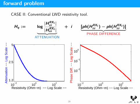
CASE II: Conventional LWD resistivity tool.
Hq := log|HRX1
zz ||HRX2zz |︸ ︷︷ ︸
ATTENUATION
+ i [ph(HRX1zz ) − ph(HRX2
zz )]︸ ︷︷ ︸PHASE DIFFERENCE
10−2
100
102
1.2
2.5
5
Resistivity (Ohm−m) −− Log Scale −−
Atte
nuat
ion
−−
Log
Sca
le −
−
10−2
100
102
10−2
10−1
100
Resistivity (Ohm−m) −− Log Scale −−
Pha
se D
iff. −
− L
og S
cale
−−
29
forward problem
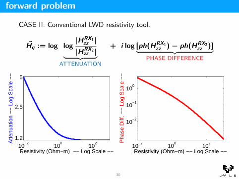
CASE II: Conventional LWD resistivity tool.
Hq := log log|HRX1
zz ||HRX2zz |︸ ︷︷ ︸
ATTENUATION
+ i log [ph(HRX1zz ) − ph(HRX2
zz )]︸ ︷︷ ︸PHASE DIFFERENCE
10−2
100
102
1.2
2.5
5
Resistivity (Ohm−m) −− Log Scale −−
Atte
nuat
ion
−−
Log
Sca
le −
−
10−2
100
102
10−2
10−1
100
Resistivity (Ohm−m) −− Log Scale −−
Pha
se D
iff. −
− L
og S
cale
−−
30
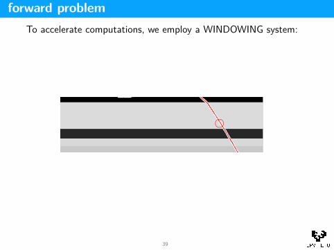
forward problemTo accelerate computations, we employ a WINDOWING system:
1000 1050 1100 1150
0
1
2
3
4
Model Problem and Well Trajectory
Horizontal Depth (m)
Tru
e V
ertic
al D
epth
(m
)
31
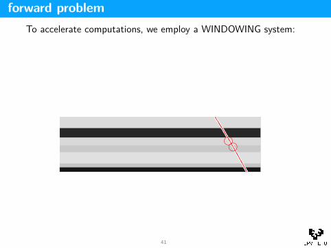
forward problemTo accelerate computations, we employ a WINDOWING system:
1000 1050 1100 1150
0
1
2
3
4
Model Problem and Well Trajectory
Horizontal Depth (m)
Tru
e V
ertic
al D
epth
(m
)
hhhhhh
32
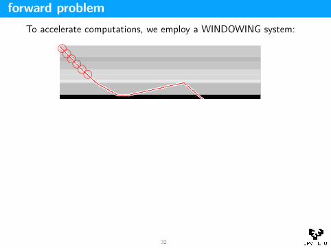
forward problemTo accelerate computations, we employ a WINDOWING system:
1000 1050 1100 1150
0
1
2
3
4
Model Problem and Well Trajectory
Horizontal Depth (m)
Tru
e V
ertic
al D
epth
(m
)
h
33
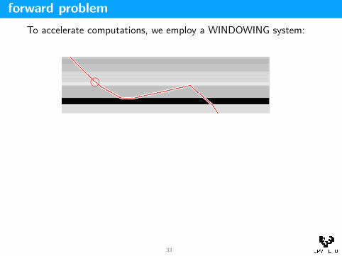
forward problemTo accelerate computations, we employ a WINDOWING system:
1000 1050 1100 1150
0
1
2
3
4
Model Problem and Well Trajectory
Horizontal Depth (m)
Tru
e V
ertic
al D
epth
(m
) hhhhhhhhhh
34
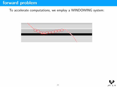
forward problemTo accelerate computations, we employ a WINDOWING system:
1000 1050 1100 1150
0
1
2
3
4
Model Problem and Well Trajectory
Horizontal Depth (m)
Tru
e V
ertic
al D
epth
(m
)
h
35
forward problemTo accelerate computations, we employ a WINDOWING system:
1000 1050 1100 1150
0
1
2
3
4
Model Problem and Well Trajectory
Horizontal Depth (m)
Tru
e V
ertic
al D
epth
(m
) hhh
36
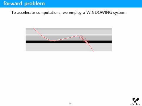
forward problemTo accelerate computations, we employ a WINDOWING system:
1000 1050 1100 1150
0
1
2
3
4
Model Problem and Well Trajectory
Horizontal Depth (m)
Tru
e V
ertic
al D
epth
(m
) h
37
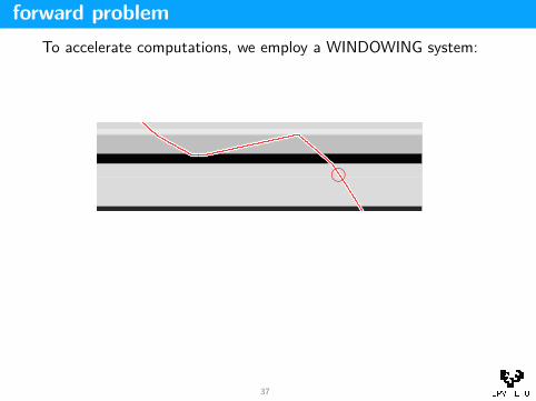
forward problemTo accelerate computations, we employ a WINDOWING system:
1000 1050 1100 1150
0
1
2
3
4
Model Problem and Well Trajectory
Horizontal Depth (m)
Tru
e V
ertic
al D
epth
(m
)
h
38
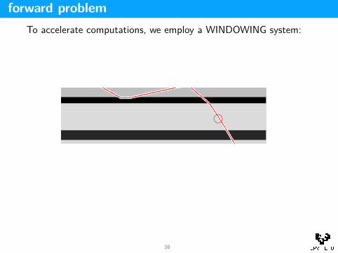
forward problemTo accelerate computations, we employ a WINDOWING system:
1000 1050 1100 1150
0
1
2
3
4
Model Problem and Well Trajectory
Horizontal Depth (m)
Tru
e V
ertic
al D
epth
(m
)
h
39
forward problemTo accelerate computations, we employ a WINDOWING system:
1000 1050 1100 1150
0
1
2
3
4
Model Problem and Well Trajectory
Horizontal Depth (m)
Tru
e V
ertic
al D
epth
(m
)
h
40
forward problemTo accelerate computations, we employ a WINDOWING system:
1000 1050 1100 1150
0
1
2
3
4
Model Problem and Well Trajectory
Horizontal Depth (m)
Tru
e V
ertic
al D
epth
(m
)
hh
41
forward problemTo accelerate computations, we employ a WINDOWING system:
1000 1050 1100 1150
0
1
2
3
4
Model Problem and Well Trajectory
Horizontal Depth (m)
Tru
e V
ertic
al D
epth
(m
)
h
42
forward problemTo accelerate computations, we employ a WINDOWING system:
1000 1050 1100 1150
0
1
2
3
4
Model Problem and Well Trajectory
Horizontal Depth (m)
Tru
e V
ertic
al D
epth
(m
)
hh
43
forward problemTo accelerate computations, we employ a WINDOWING system:
1000 1050 1100 1150
0
1
2
3
4
Model Problem and Well Trajectory
Horizontal Depth (m)
Tru
e V
ertic
al D
epth
(m
)
hhh
44
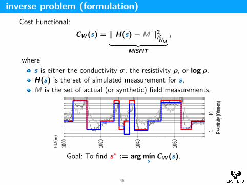
inverse problem (formulation)Cost Functional:
CW (s) = ‖ H(s) − M ‖2l2WM︸ ︷︷ ︸
MISFIT
,
wheres is either the conductivity σ, the resistivity ρ, or log ρ,H(s) is the set of simulated measurement for s,M is the set of actual (or synthetic) field measurements,
HD
(m)
110
1000
1020
1040
1060
Resis
tivity
(Ohm
-m)
Goal: To find s∗ := arg mıns
CW (s).
45
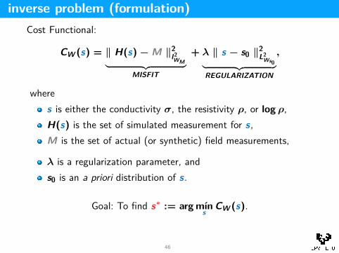
inverse problem (formulation)Cost Functional:
CW (s) = ‖ H(s) − M ‖2l2WM︸ ︷︷ ︸
MISFIT
+ λ ‖ s − s0 ‖2L2
Ws0︸ ︷︷ ︸REGULARIZATION
,
wheres is either the conductivity σ, the resistivity ρ, or log ρ,H(s) is the set of simulated measurement for s,M is the set of actual (or synthetic) field measurements,
λ is a regularization parameter, ands0 is an a priori distribution of s.
Goal: To find s∗ := arg mıns
CW (s).
46
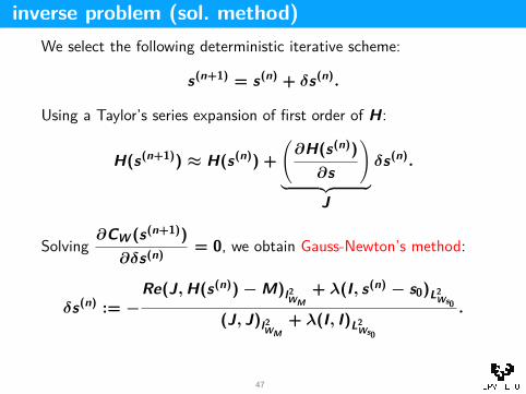
inverse problem (sol. method)We select the following deterministic iterative scheme:
s(n+1) = s(n) + δs(n).
Using a Taylor’s series expansion of first order of H:
H(s(n+1)) ≈ H(s(n)) +(
∂H(s(n))∂s
)︸ ︷︷ ︸
J
δs(n).
Solving∂CW (s(n+1))
∂δs(n)= 0, we obtain Gauss-Newton’s method:
δs(n) := −Re(J, H(s(n)) − M)l2
WM+ λ(I, s(n) − s0)L2
Ws0
(J, J)l2WM
+ λ(I, I)L2Ws0
.
47
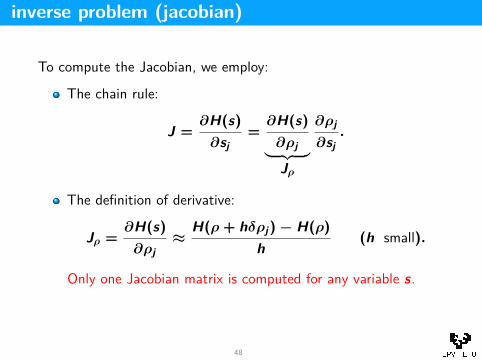
inverse problem (jacobian)
To compute the Jacobian, we employ:
The chain rule:
J =∂H(s)
∂sj=
∂H(s)∂ρj︸ ︷︷ ︸Jρ
∂ρj
∂sj.
The definition of derivative:
Jρ =∂H(s)
∂ρj≈
H(ρ + hδρj) − H(ρ)
h(h small).
Only one Jacobian matrix is computed for any variable s.
48
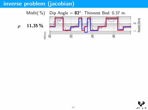
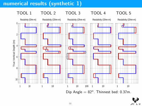
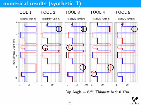
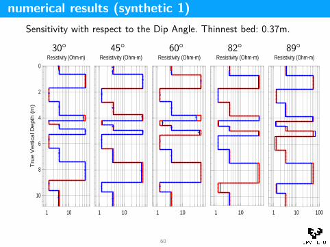
inverse problem (jacobian)Misfit( %) Dip Angle = 82◦. Thinnest Bed: 0.37 m.
ρ
σ
log ρ
Best
11,35%
11,32%
7,87%
6,58%
HD
(m) 1
10
1000
1020
1040
1060
Resist
ivity (O
hm-m)
110
100
1000
1020
1040
1060
Resistiv
ity (Oh
m-m)
110
1000
1020
1040
1060
Resistiv
ity (Oh
m-m)
110
1000
1020
1040
1060
Resistiv
ity (Oh
m-m)
������������mnn
mnnmnn
mnnmnn
49
inverse problem (jacobian)Misfit( %) Dip Angle = 82◦. Thinnest Bed: 0.37 m.
ρ
σ
log ρ
Best
11,35%
11,32%
7,87%
6,58%
HD
(m) 1
10
1000
1020
1040
1060
Resist
ivity (O
hm-m)
110
100
1000
1020
1040
1060
Resistiv
ity (Oh
m-m)
110
1000
1020
1040
1060
Resistiv
ity (Oh
m-m)
110
1000
1020
1040
1060
Resistiv
ity (Oh
m-m)
������������
mnnmnn
mnnmnn
mnn
50
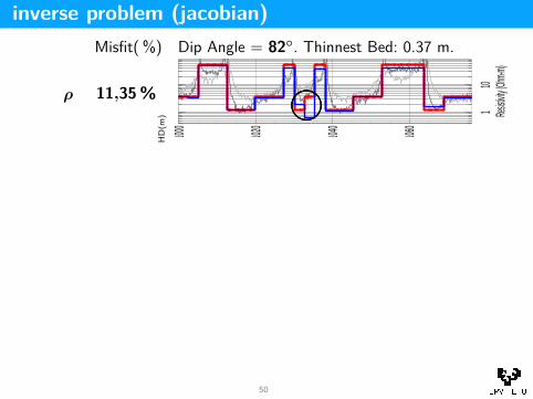
inverse problem (jacobian)Misfit( %) Dip Angle = 82◦. Thinnest Bed: 0.37 m.
ρ
σ
log ρ
Best
11,35%
11,32%
7,87%
6,58%
HD
(m) 1
10
1000
1020
1040
1060
Resist
ivity (O
hm-m)
110
100
1000
1020
1040
1060
Resistiv
ity (Oh
m-m)
110
1000
1020
1040
1060
Resistiv
ity (Oh
m-m)
110
1000
1020
1040
1060
Resistiv
ity (Oh
m-m)
������������
mnnmnn
mnnmnn
mnn
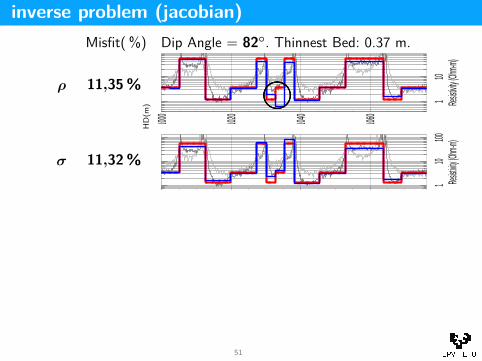
51
inverse problem (jacobian)Misfit( %) Dip Angle = 82◦. Thinnest Bed: 0.37 m.
ρ
σ
log ρ
Best
11,35%
11,32%
7,87%
6,58%
HD
(m) 1
10
1000
1020
1040
1060
Resist
ivity (O
hm-m)
110
100
1000
1020
1040
1060
Resistiv
ity (Oh
m-m)
110
1000
1020
1040
1060
Resistiv
ity (Oh
m-m)
110
1000
1020
1040
1060
Resistiv
ity (Oh
m-m)
������������mnn
mnnmnn
mnnmnn
52
inverse problem (jacobian)Misfit( %) Dip Angle = 82◦. Thinnest Bed: 0.37 m.
ρ
σ
log ρ
Best
11,35%
11,32%
7,87%
6,58%
HD
(m) 1
10
1000
1020
1040
1060
Resist
ivity (O
hm-m)
110
100
1000
1020
1040
1060
Resistiv
ity (Oh
m-m)
110
1000
1020
1040
1060
Resistiv
ity (Oh
m-m)
110
1000
1020
1040
1060
Resistiv
ity (Oh
m-m)
������������mnn
mnnmnn
mnnmnn
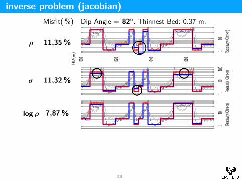
53
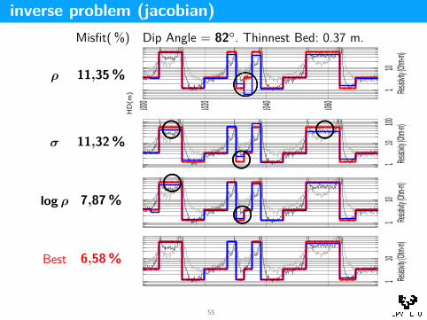
inverse problem (jacobian)Misfit( %) Dip Angle = 82◦. Thinnest Bed: 0.37 m.
ρ
σ
log ρ
Best
11,35%
11,32%
7,87%
6,58%
HD
(m) 1
10
1000
1020
1040
1060
Resist
ivity (O
hm-m)
110
100
1000
1020
1040
1060
Resistiv
ity (Oh
m-m)
110
1000
1020
1040
1060
Resistiv
ity (Oh
m-m)
110
1000
1020
1040
1060
Resistiv
ity (Oh
m-m)
������������mnn
mnnmnn
mnnmnn
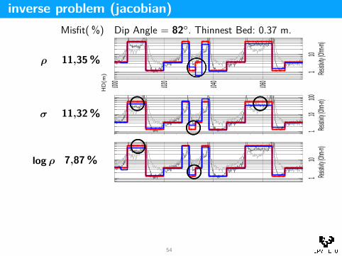
54
inverse problem (jacobian)Misfit( %) Dip Angle = 82◦. Thinnest Bed: 0.37 m.
ρ
σ
log ρ
Best
11,35%
11,32%
7,87%
6,58%
HD
(m) 1
10
1000
1020
1040
1060
Resist
ivity (O
hm-m)
110
100
1000
1020
1040
1060
Resistiv
ity (Oh
m-m)
110
1000
1020
1040
1060
Resistiv
ity (Oh
m-m)
110
1000
1020
1040
1060
Resistiv
ity (Oh
m-m)
������������mnn
mnnmnn
mnnmnn
55
inverse problem (error bars)
Once we achieve convergence, we have:
δs(n) ≈ 0.
Considering new noisy measurements of the type:
M := M + N
and using these new measurements in our Gauss-Newton method,we obtain the following new correction δs(n):
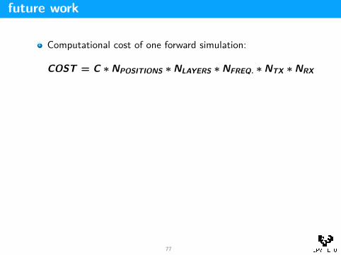
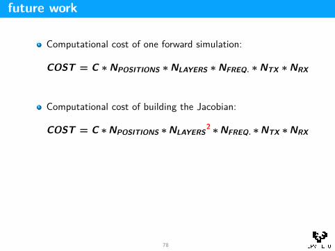
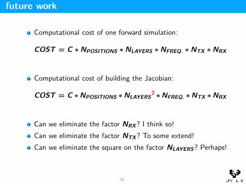
Can we eliminate the factor NRX? I think so!Can we eliminate the factor NTX? To some extend!Can we eliminate the square on the factor NLAYERS? Perhaps!
Can we eliminate the factor NRX? I think so!Can we eliminate the factor NTX? To some extend!Can we eliminate the square on the factor NLAYERS? Perhaps!
Can we eliminate the factor NRX? I think so!Can we eliminate the factor NTX? To some extend!Can we eliminate the square on the factor NLAYERS? Perhaps!
79
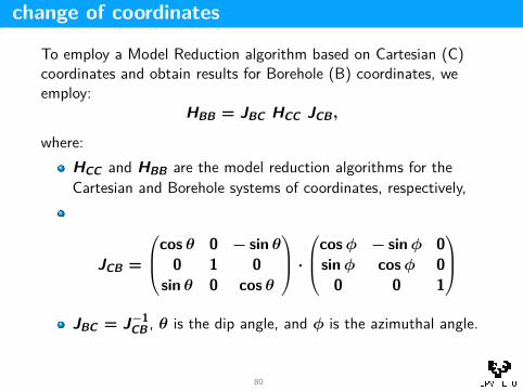
change of coordinates
To employ a Model Reduction algorithm based on Cartesian (C)coordinates and obtain results for Borehole (B) coordinates, weemploy:
HBB = JBC HCC JCB,
where:HCC and HBB are the model reduction algorithms for theCartesian and Borehole systems of coordinates, respectively,
JCB =
cos θ 0 − sin θ
0 1 0sin θ 0 cos θ
·
cos φ − sin φ 0sin φ cos φ 0
0 0 1
JBC = J−1
CB , θ is the dip angle, and φ is the azimuthal angle.
80
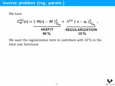
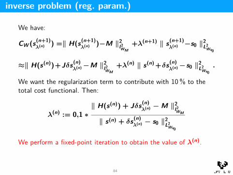
inverse problem (reg. param.)
We have:
C (n)W (s) = ‖ H(s) − M ‖2
l2WM︸ ︷︷ ︸
MISFIT
+ λ(n) ‖ s − s0 ‖2L2
Ws0︸ ︷︷ ︸REGULARIZATION
,
90% 10%
We want the regularization term to contribute with 10 % to thetotal cost functional. Then:
λ(n) := 0,1 ∗‖ H(s(n)) + Jδs(n)
λ(n) − M ‖2l2WM
‖ s(n) + δs(n)λ(n) − s0 ‖2
L2Ws0
We perform a fixed-point iteration to obtain the value of λ(n).
81
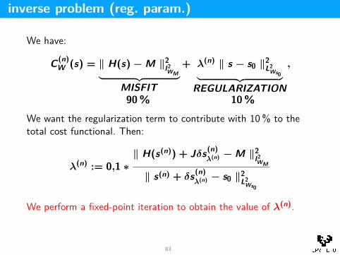
inverse problem (reg. param.)
We have:
C (n)W (s) = ‖ H(s) − M ‖2
l2WM︸ ︷︷ ︸
MISFIT
+ λ(n) ‖ s − s0 ‖2L2
Ws0︸ ︷︷ ︸REGULARIZATION
,
90% 10%
We want the regularization term to contribute with 10 % to thetotal cost functional.
Then:
λ(n) := 0,1 ∗‖ H(s(n)) + Jδs(n)
λ(n) − M ‖2l2WM
‖ s(n) + δs(n)λ(n) − s0 ‖2
L2Ws0
We perform a fixed-point iteration to obtain the value of λ(n).
82
inverse problem (reg. param.)
We have:
C (n)W (s) = ‖ H(s) − M ‖2
l2WM︸ ︷︷ ︸
MISFIT
+ λ(n) ‖ s − s0 ‖2L2
Ws0︸ ︷︷ ︸REGULARIZATION
,
90% 10%
We want the regularization term to contribute with 10 % to thetotal cost functional. Then:
λ(n) := 0,1 ∗‖ H(s(n)) + Jδs(n)
λ(n) − M ‖2l2WM
‖ s(n) + δs(n)λ(n) − s0 ‖2
L2Ws0
We perform a fixed-point iteration to obtain the value of λ(n).
83
inverse problem (reg. param.)
We have:
CW (s(n+1)λ(n) ) =‖ H(s(n+1)
λ(n) )−M ‖2l2WM
+λ(n+1) ‖ s(n+1)λ(n) −s0 ‖2
L2Ws0
≈‖ H(s(n))+Jδs(n)λ(n) −M ‖2
l2WM
+λ(n) ‖ s(n)+δs(n)λ(n) −s0 ‖2
L2Ws0
.
We want the regularization term to contribute with 10 % to thetotal cost functional. Then:
λ(n) := 0,1 ∗‖ H(s(n)) + Jδs(n)
λ(n) − M ‖2l2WM
‖ s(n) + δs(n)λ(n) − s0 ‖2
L2Ws0
We perform a fixed-point iteration to obtain the value of λ(n).
84
inverse p. (stopping criteria)
We stop the inversion process when both the relative data misfitand regularization term do not vary significantly. Mathematically,we require the following two conditions to be satisfied:
100∗| ‖ H(s(n+1)) − M ‖2
l2WM
− ‖ H(s(n)) − M ‖2l2WM
|
‖ M ‖2l2WM
≤ 0,5%
And:
100λ(n) ∗| ‖ s(n+1) − s0 ‖2
L2Ws0
− ‖ s(n) − s0 ‖2L2
Ws0
|
‖ s0 ‖2L2
Ws0
≤ 5%.
85
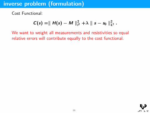
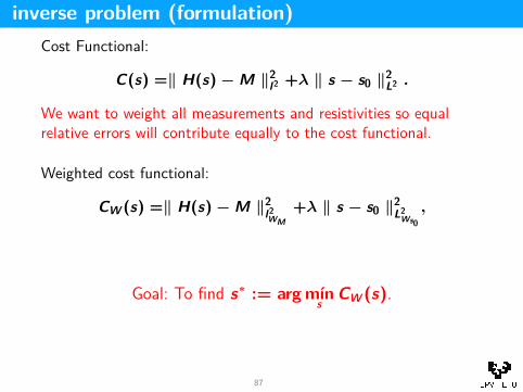
inverse problem (formulation)Cost Functional:
C(s) =‖ H(s) − M ‖2l2 +λ ‖ s − s0 ‖2
L2 .
We want to weight all measurements and resistivities so equalrelative errors will contribute equally to the cost functional.
Weighted cost functional:
CW (s) =‖ H(s) − M ‖2l2WM
+λ ‖ s − s0 ‖2L2
Ws0,
Goal: To find s∗ := arg mıns
CW (s).
86
inverse problem (formulation)Cost Functional:
C(s) =‖ H(s) − M ‖2l2 +λ ‖ s − s0 ‖2
L2 .
We want to weight all measurements and resistivities so equalrelative errors will contribute equally to the cost functional.


![[p.T] Modeling and Inversion Methods for the Interpretation of Resistivity Logging Tool Response](https://static.documents.pub/doc/80x56/577d34871a28ab3a6b8e3c14/pt-modeling-and-inversion-methods-for-the-interpretation-of-resistivity.jpg)


