Fast Iterative Solution of Saddle Point Problems Fast Iterative Solution of Saddle Point Problems Michele Benzi Department of Mathematics and Computer Science Emory University Atlanta, GA December 1, 2016
Transcript
Fast Iterative Solution of Saddle Point Problems
Fast Iterative Solution of Saddle Point Problems
Michele Benzi
Department of Mathematics and Computer ScienceEmory University
Atlanta, GA
December 1, 2016
Fast Iterative Solution of Saddle Point Problems
Acknowledgments
NSF (Computational Mathematics)
Maxim Olshanskii (Mech-Math, Moscow State U.)
Zhen Wang (former PhD student, Emory U.; currently at ORNL)
Thanks also to Valeria Simoncini (U. of Bologna, Italy)
Fast Iterative Solution of Saddle Point Problems
Motivation and goals
Let A be a real, symmetric, n × n matrix and let f ∈ Rn be given.
Let 〈·, ·〉 denote the standard inner product in Rn.
Consider the following two problems:
1 Solve Au = f
2 Minimize the function J(u) = 12〈Au, u〉 − 〈f , u〉
Note that ∇J(u) = Au − f . Hence, if A is positive definite (SPD), the twoproblems are equivalent, and there exists a unique solution u∗ = A−1f .
Many algorithms exist for solving SPD linear systems: Cholesky, PreconditionedConjugate Gradients, AMG, etc.
Fast Iterative Solution of Saddle Point Problems
Motivation and goals (cont.)
Now we add a set of linear constraints:
Minimize J(u) = 12〈Au, u〉 − 〈f , u〉
subject to Bu = g
where
A is n × n, symmetric
B is m × n, with m < n
f ∈ Rn, g ∈ Rm are given (either f or g could be 0, but not both)
Standard approach: Introduce Lagrange multipliers, p ∈ Rm
Mixed FEM formulations of 2nd- and 4th-order elliptic PDEs
Time-harmonic Maxwell equations
PDE-constrained optimization (e.g., variational data assimilation)
SQP and IP methods for nonlinear constrained optimization
Structural analysis
Resistive networks, power network analysis
Certain economic models
Comprehensive survey: M. Benzi, G. Golub and J. Liesen, Numerical solution ofsaddle point problems, Acta Numerica 14 (2005), pp. 1–137.
The bibliography in this paper contains 535 items.
Google Scholar reports 1467 citations as of 12/01/2016.
Fast Iterative Solution of Saddle Point Problems
Motivation and goals (cont.)
The aim of this lecture:
To briefly review the basic properties of saddle point systems
To give an overview of solution algorithms for specific problems
To point out some current challenges and recent developments
The emphasis of the lecture will be on preconditioned iterative solvers for large,sparse saddle point problems, with a focus on our own recent work onpreconditioners for incompressible flow problems.
The ultimate goal: to develop robust preconditioners that perform uniformlywell independently of discretization details and problem parameters.
For flow problems, we would like to have solvers that converge fast regardlessof mesh size, viscosity, etc. Moreover, the cost per iteration should be linear inthe number of unknowns.
Fast Iterative Solution of Saddle Point Problems
Outline
Fast Iterative Solution of Saddle Point Problems
Properties of saddle point matrices
Outline
Fast Iterative Solution of Saddle Point Problems
Properties of saddle point matrices
Solvability of saddle point problems
The following result establishes necessary and sufficient conditions for theunique solvability of the saddle point problem (1).
Theorem. Assume that
A is symmetric positive semidefinite n × n
B has full rank: rank (B) = m
Then the coefficient matrix
A =
„A BT
B O
«is nonsingular ⇔ Null (A) ∩ Null (B) = 0.
Furthermore, A is indefinite, with n positive and m negative eigenvalues.
In particular, A is invertible if A is SPD and B has full rank (“standard case”).
Fast Iterative Solution of Saddle Point Problems
Properties of saddle point matrices
Generalizations, I
In some cases, a stabilization (or regularization) term needs to be added in the(2,2) position, leading to linear systems of the form
„A BT
B −βC
«„up
«=
„fg
«(2)
where β > 0 is a small parameter and the m ×m matrix C is symmetricpositive semidefinite, and often singular, with ‖C‖2 = 1.
This type of system arises, for example, from the stabilization of FEM pairsthat do not satisfy the LBB (‘inf-sup’) condition.
Another important example is the discretization of the Reissner–Mindlin platemodel in linear elasticity. In this case β is related to the thickness of the plate;the limit case β = 0 can be seen as a reformulation of the biharmonic problem.
Fast Iterative Solution of Saddle Point Problems
Properties of saddle point matrices
Generalizations, I
In some cases, a stabilization (or regularization) term needs to be added in the(2,2) position, leading to linear systems of the form„
A BT
B −βC
«„up
«=
„fg
«(2)
where β > 0 is a small parameter and the m ×m matrix C is symmetricpositive semidefinite, and often singular, with ‖C‖2 = 1.
This type of system arises, for example, from the stabilization of FEM pairsthat do not satisfy the LBB (‘inf-sup’) condition.
Another important example is the discretization of the Reissner–Mindlin platemodel in linear elasticity. In this case β is related to the thickness of the plate;the limit case β = 0 can be seen as a reformulation of the biharmonic problem.
Fast Iterative Solution of Saddle Point Problems
Properties of saddle point matrices
Generalizations, II
In other cases, the matrix A is not symmetric: A 6= AT . In this case, the saddlepoint system does not arise from a constrained minimization problem.
The most important examples of this case are linear systems arising from thePicard and Newton linearizations of the steady incompressible Navier–Stokesequations. The following result is applicable to the Picard linearization (Oseenproblem):
Theorem. Assume that
H = 12(A + AT ) is symmetric positive semidefinite n × n
B has full rank: rank (B) = m
Then
Null(H) ∩ Null(B) = 0 ⇒ A invertible
A invertible ⇒ Null(A) ∩ Null(B) = 0.
Fast Iterative Solution of Saddle Point Problems
Properties of saddle point matrices
Nonsymmetric, positive definite form
Consider the following equivalent formulation:
„A BT
−B O
«„up
«=
„f−g
«
Theorem. Assume B has full rank. If H = 12(A + AT ) is positive definite, then
the spectrum of
A− :=
„A BT
−B O
«lies entirely in the open right-half plane Re(z) > 0. Moreover, if A is SPD andthe following condition holds:
λmin(A) > 4λmax(S) where S = BA−1BT (“Schur complement”),
then A− is diagonalizable with real positive eigenvalues. In this case, thereexists a non-standard inner product on Rn+m in which A− is self-adjoint andpositive definite, and a corresponding conjugate gradient method(B./Simoncini, NM 2006).
Fast Iterative Solution of Saddle Point Problems
Properties of saddle point matrices
Nonsymmetric, positive definite form
Consider the following equivalent formulation:
„A BT
−B O
«„up
«=
„f−g
«
Theorem. Assume B has full rank. If H = 12(A + AT ) is positive definite, then
the spectrum of
A− :=
„A BT
−B O
«lies entirely in the open right-half plane Re(z) > 0. Moreover, if A is SPD andthe following condition holds:
λmin(A) > 4λmax(S) where S = BA−1BT (“Schur complement”),
then A− is diagonalizable with real positive eigenvalues.
In this case, thereexists a non-standard inner product on Rn+m in which A− is self-adjoint andpositive definite, and a corresponding conjugate gradient method(B./Simoncini, NM 2006).
Fast Iterative Solution of Saddle Point Problems
Properties of saddle point matrices
Nonsymmetric, positive definite form
Consider the following equivalent formulation:
„A BT
−B O
«„up
«=
„f−g
«
Theorem. Assume B has full rank. If H = 12(A + AT ) is positive definite, then
the spectrum of
A− :=
„A BT
−B O
«lies entirely in the open right-half plane Re(z) > 0. Moreover, if A is SPD andthe following condition holds:
λmin(A) > 4λmax(S) where S = BA−1BT (“Schur complement”),
then A− is diagonalizable with real positive eigenvalues. In this case, thereexists a non-standard inner product on Rn+m in which A− is self-adjoint andpositive definite, and a corresponding conjugate gradient method(B./Simoncini, NM 2006).
Fast Iterative Solution of Saddle Point Problems
Examples: Incompressible flow problems
Outline
Fast Iterative Solution of Saddle Point Problems
Examples: Incompressible flow problems
Example 1: the generalized Stokes problem
Let Ω be a domain in Rd and let α ≥ 0, ν > 0. Consider the system
αu− ν∆u +∇p = f in Ω,
div u = 0 in Ω,
u = 0 on ∂Ω.
Weak formulation: Find (u, p) ∈ (H10 (Ω))d × L2
0(Ω) such that
α〈u, v〉+ 〈∇u,∇v〉 − 〈p, div v〉 = 〈f, v〉, v ∈ (H10 (Ω))d ,
〈q, div u〉 = 0, q ∈ L20(Ω),
where 〈·, ·〉 denotes the L2 inner product.
The standard Stokes problem is obtained for α = 0 (steady case). In this casewe can assume ν = 1.
Fast Iterative Solution of Saddle Point Problems
Examples: Incompressible flow problems
Example 1: the generalized Stokes problem (cont.)
Discretization using LBB-stable finite element pairs or other div-stable schemeleads to an algebraic saddle point problem:
„A BT
B O
«„up
«=
„f0
«
Here A is a discrete reaction-diffusion operator, BT the discrete gradient, andB the discrete (negative) divergence. For α = 0, A is just the discrete vectorLaplacian.
If an unstable FEM pair is used, then a regularization term −βC is added inthe (2, 2) block of A. The specific choice of β and C depends on the particulardiscretization used.
Robust, optimal solvers have been developed for this problem:Cahouet–Chabard for α > 0; Silvester–Wathen for α = 0.
Fast Iterative Solution of Saddle Point Problems
Examples: Incompressible flow problems
Example 1: the generalized Stokes problem (cont.)
Discretization using LBB-stable finite element pairs or other div-stable schemeleads to an algebraic saddle point problem:„
A BT
B O
«„up
«=
„f0
«
Here A is a discrete reaction-diffusion operator, BT the discrete gradient, andB the discrete (negative) divergence. For α = 0, A is just the discrete vectorLaplacian.
If an unstable FEM pair is used, then a regularization term −βC is added inthe (2, 2) block of A. The specific choice of β and C depends on the particulardiscretization used.
Robust, optimal solvers have been developed for this problem:Cahouet–Chabard for α > 0; Silvester–Wathen for α = 0.
Fast Iterative Solution of Saddle Point Problems
Examples: Incompressible flow problems
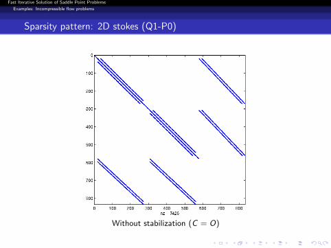
Sparsity pattern: 2D stokes (Q1-P0)
Without stabilization (C = O)
Fast Iterative Solution of Saddle Point Problems
Examples: Incompressible flow problems
Sparsity pattern: 2D stokes (Q1-P0)
With stabilization (C 6= O)
Fast Iterative Solution of Saddle Point Problems
Examples: Incompressible flow problems
Example 2: the generalized Oseen problem
Let Ω be a domain in Rd and let α ≥ 0 and ν > 0. Also, let w be adivergence-free vector field on Ω. Consider the system
αu− ν∆u + (w · ∇) u +∇p = f in Ω,
div u = 0 in Ω,
u = 0 on ∂Ω.
Note that for w = 0 we recover the generalized Stokes problem.
Weak formulation: Find (u, p) ∈ (H10 (Ω))d × L2
0(Ω) such that
α〈u, v〉+ ν〈∇u,∇v〉+ 〈(w · ∇) u, v〉 − 〈p, div v〉 = 〈f, v〉, v ∈ (H10 (Ω))d ,
〈q, div u〉 = 0, q ∈ L20(Ω).
The standard Oseen problem is obtained for α = 0 (steady case).
Fast Iterative Solution of Saddle Point Problems
Examples: Incompressible flow problems
Example 2: the generalized Oseen problem (cont.)
Discretization using LBB-stable finite element pairs or other div-stable schemeleads to an algebraic saddle point problem:
„A BT
B O
«„up
«=
„f0
«
Now A is a discrete reaction-convection-diffusion operator. For α = 0, A is justa discrete vector convection-diffusion operator. Note that now A 6= AT .
The Oseen problem arises from Picard iteration applied to the steadyincompressible Navier–Stokes equations, and from fully implicit schemesapplied to the unsteady NSE. The ‘wind’ w represents an approximation of thesolution u obtained from the previous Picard step, or from time-lagging.
As we will see, this problem can be very challenging to solve, especially forsmall values of the viscosity ν and on stretched meshes.
Fast Iterative Solution of Saddle Point Problems
Examples: Incompressible flow problems
Example 2: the generalized Oseen problem (cont.)
Discretization using LBB-stable finite element pairs or other div-stable schemeleads to an algebraic saddle point problem:„
A BT
B O
«„up
«=
„f0
«
Now A is a discrete reaction-convection-diffusion operator. For α = 0, A is justa discrete vector convection-diffusion operator. Note that now A 6= AT .
The Oseen problem arises from Picard iteration applied to the steadyincompressible Navier–Stokes equations, and from fully implicit schemesapplied to the unsteady NSE. The ‘wind’ w represents an approximation of thesolution u obtained from the previous Picard step, or from time-lagging.
As we will see, this problem can be very challenging to solve, especially forsmall values of the viscosity ν and on stretched meshes.
Fast Iterative Solution of Saddle Point Problems
Examples: Incompressible flow problems
Eigenvalues of discrete Oseen problem (ν = 0.01), indefinite form
Eigenvalues of Oseen matrix A =
„A BT
B O
«, MAC discretization.
−50 0 50 100 150 200 250−4
−3
−2
−1
0
1
2
3
4
Note the different scales in the x and y axes.
Fast Iterative Solution of Saddle Point Problems
Examples: Incompressible flow problems
Eigenvalues of discrete Oseen problem (ν = 0.01), positive definite form
Eigenvalues of Oseen matrix A− =
„A BT
−B O
«, MAC discretization.
0 20 40 60 80 100 120 140 160 180 200−6
−4
−2
0
2
4
6
Note the different scales in the x and y axes.
Fast Iterative Solution of Saddle Point Problems
Some solution algorithms
Outline
Fast Iterative Solution of Saddle Point Problems
Some solution algorithms
Overview of available solvers
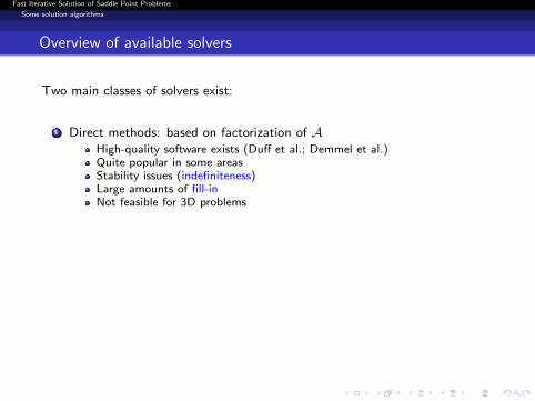
Two main classes of solvers exist:
1 Direct methods: based on factorization of A
High-quality software exists (Duff et al.; Demmel et al.)Quite popular in some areasStability issues (indefiniteness)Large amounts of fill-inNot feasible for 3D problemsDifficult to parallelize
2 Krylov subspace methods (MINRES, GMRES, Bi-CGSTAB,...)Appropriate for large, sparse problemsTend to converge slowlyNumber of iterations increases as problem size growsEffective preconditioners a must
Much effort has been put into developing preconditioners, with optimality androbustness w.r.t. parameters as the ultimate goals. Parallelizability also needsto be taken into account.
Fast Iterative Solution of Saddle Point Problems
Some solution algorithms
Overview of available solvers
Two main classes of solvers exist:
1 Direct methods: based on factorization of AHigh-quality software exists (Duff et al.; Demmel et al.)
Quite popular in some areasStability issues (indefiniteness)Large amounts of fill-inNot feasible for 3D problemsDifficult to parallelize
2 Krylov subspace methods (MINRES, GMRES, Bi-CGSTAB,...)Appropriate for large, sparse problemsTend to converge slowlyNumber of iterations increases as problem size growsEffective preconditioners a must
Much effort has been put into developing preconditioners, with optimality androbustness w.r.t. parameters as the ultimate goals. Parallelizability also needsto be taken into account.
Fast Iterative Solution of Saddle Point Problems
Some solution algorithms
Overview of available solvers
Two main classes of solvers exist:
1 Direct methods: based on factorization of AHigh-quality software exists (Duff et al.; Demmel et al.)Quite popular in some areas
Stability issues (indefiniteness)Large amounts of fill-inNot feasible for 3D problemsDifficult to parallelize
2 Krylov subspace methods (MINRES, GMRES, Bi-CGSTAB,...)Appropriate for large, sparse problemsTend to converge slowlyNumber of iterations increases as problem size growsEffective preconditioners a must
Much effort has been put into developing preconditioners, with optimality androbustness w.r.t. parameters as the ultimate goals. Parallelizability also needsto be taken into account.
Fast Iterative Solution of Saddle Point Problems
Some solution algorithms
Overview of available solvers
Two main classes of solvers exist:
1 Direct methods: based on factorization of AHigh-quality software exists (Duff et al.; Demmel et al.)Quite popular in some areasStability issues (indefiniteness)
Large amounts of fill-inNot feasible for 3D problemsDifficult to parallelize
2 Krylov subspace methods (MINRES, GMRES, Bi-CGSTAB,...)Appropriate for large, sparse problemsTend to converge slowlyNumber of iterations increases as problem size growsEffective preconditioners a must
Much effort has been put into developing preconditioners, with optimality androbustness w.r.t. parameters as the ultimate goals. Parallelizability also needsto be taken into account.
Fast Iterative Solution of Saddle Point Problems
Some solution algorithms
Overview of available solvers
Two main classes of solvers exist:
1 Direct methods: based on factorization of AHigh-quality software exists (Duff et al.; Demmel et al.)Quite popular in some areasStability issues (indefiniteness)Large amounts of fill-in
Not feasible for 3D problemsDifficult to parallelize
2 Krylov subspace methods (MINRES, GMRES, Bi-CGSTAB,...)Appropriate for large, sparse problemsTend to converge slowlyNumber of iterations increases as problem size growsEffective preconditioners a must
Much effort has been put into developing preconditioners, with optimality androbustness w.r.t. parameters as the ultimate goals. Parallelizability also needsto be taken into account.
Fast Iterative Solution of Saddle Point Problems
Some solution algorithms
Overview of available solvers
Two main classes of solvers exist:
1 Direct methods: based on factorization of AHigh-quality software exists (Duff et al.; Demmel et al.)Quite popular in some areasStability issues (indefiniteness)Large amounts of fill-inNot feasible for 3D problems
Difficult to parallelize
2 Krylov subspace methods (MINRES, GMRES, Bi-CGSTAB,...)Appropriate for large, sparse problemsTend to converge slowlyNumber of iterations increases as problem size growsEffective preconditioners a must
Much effort has been put into developing preconditioners, with optimality androbustness w.r.t. parameters as the ultimate goals. Parallelizability also needsto be taken into account.
Fast Iterative Solution of Saddle Point Problems
Some solution algorithms
Overview of available solvers
Two main classes of solvers exist:
1 Direct methods: based on factorization of AHigh-quality software exists (Duff et al.; Demmel et al.)Quite popular in some areasStability issues (indefiniteness)Large amounts of fill-inNot feasible for 3D problemsDifficult to parallelize
Appropriate for large, sparse problemsTend to converge slowlyNumber of iterations increases as problem size growsEffective preconditioners a must
Much effort has been put into developing preconditioners, with optimality androbustness w.r.t. parameters as the ultimate goals. Parallelizability also needsto be taken into account.
Fast Iterative Solution of Saddle Point Problems
Some solution algorithms
Overview of available solvers
Two main classes of solvers exist:
1 Direct methods: based on factorization of AHigh-quality software exists (Duff et al.; Demmel et al.)Quite popular in some areasStability issues (indefiniteness)Large amounts of fill-inNot feasible for 3D problemsDifficult to parallelize
Tend to converge slowlyNumber of iterations increases as problem size growsEffective preconditioners a must
Much effort has been put into developing preconditioners, with optimality androbustness w.r.t. parameters as the ultimate goals. Parallelizability also needsto be taken into account.
Fast Iterative Solution of Saddle Point Problems
Some solution algorithms
Overview of available solvers
Two main classes of solvers exist:
1 Direct methods: based on factorization of AHigh-quality software exists (Duff et al.; Demmel et al.)Quite popular in some areasStability issues (indefiniteness)Large amounts of fill-inNot feasible for 3D problemsDifficult to parallelize
2 Krylov subspace methods (MINRES, GMRES, Bi-CGSTAB,...)Appropriate for large, sparse problemsTend to converge slowly
Number of iterations increases as problem size growsEffective preconditioners a must
Much effort has been put into developing preconditioners, with optimality androbustness w.r.t. parameters as the ultimate goals. Parallelizability also needsto be taken into account.
Fast Iterative Solution of Saddle Point Problems
Some solution algorithms
Overview of available solvers
Two main classes of solvers exist:
1 Direct methods: based on factorization of AHigh-quality software exists (Duff et al.; Demmel et al.)Quite popular in some areasStability issues (indefiniteness)Large amounts of fill-inNot feasible for 3D problemsDifficult to parallelize
2 Krylov subspace methods (MINRES, GMRES, Bi-CGSTAB,...)Appropriate for large, sparse problemsTend to converge slowlyNumber of iterations increases as problem size grows
Effective preconditioners a must
Much effort has been put into developing preconditioners, with optimality androbustness w.r.t. parameters as the ultimate goals. Parallelizability also needsto be taken into account.
Fast Iterative Solution of Saddle Point Problems
Some solution algorithms
Overview of available solvers
Two main classes of solvers exist:
1 Direct methods: based on factorization of AHigh-quality software exists (Duff et al.; Demmel et al.)Quite popular in some areasStability issues (indefiniteness)Large amounts of fill-inNot feasible for 3D problemsDifficult to parallelize
2 Krylov subspace methods (MINRES, GMRES, Bi-CGSTAB,...)Appropriate for large, sparse problemsTend to converge slowlyNumber of iterations increases as problem size growsEffective preconditioners a must
Much effort has been put into developing preconditioners, with optimality androbustness w.r.t. parameters as the ultimate goals. Parallelizability also needsto be taken into account.
Fast Iterative Solution of Saddle Point Problems
Some solution algorithms
Overview of available solvers
Two main classes of solvers exist:
1 Direct methods: based on factorization of AHigh-quality software exists (Duff et al.; Demmel et al.)Quite popular in some areasStability issues (indefiniteness)Large amounts of fill-inNot feasible for 3D problemsDifficult to parallelize
2 Krylov subspace methods (MINRES, GMRES, Bi-CGSTAB,...)Appropriate for large, sparse problemsTend to converge slowlyNumber of iterations increases as problem size growsEffective preconditioners a must
Much effort has been put into developing preconditioners, with optimality androbustness w.r.t. parameters as the ultimate goals. Parallelizability also needsto be taken into account.
Fast Iterative Solution of Saddle Point Problems
Some solution algorithms
Preconditioners
Preconditioning: Find an invertible matrix P such that Krylov methodsapplied to the preconditioned system
P−1A x = P−1b
will converge rapidly (possibly, independently of the discretization parameter h).
In practice, fast convergence is typically observed when the eigenvalues of thepreconditioned matrix P−1A are clustered away from zero. However, it is notan easy matter to characterize the rate of convergence, in general.
To be effective, a preconditioner must significantly reduce the total amount ofwork:
Setting up P must be inexpensive
Evaluating z = P−1r must be inexpensive
Convergence must be rapid
Fast Iterative Solution of Saddle Point Problems
Some solution algorithms
Preconditioners
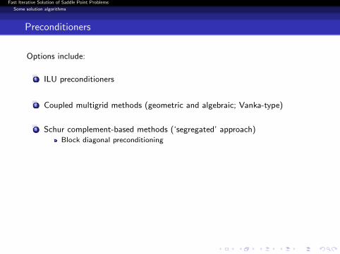
Options include:
1 ILU preconditioners
2 Coupled multigrid methods (geometric and algebraic; Vanka-type)
4 Constraint preconditioning (‘null space methods’)
5 Augmented Lagrangian-based techniques (AL)
The choice of an appropriate preconditioner is highly problem-dependent.
Fast Iterative Solution of Saddle Point Problems
Some solution algorithms
Preconditioners (cont.)
Example: The Silvester–Wathen preconditioner for the Stokes problem is
P =
bA O
O bMp
!
where bA−1 is given by a multigrid V-cycle applied to linear systems withcoefficient matrix A and bMp is the diagonal of the pressure mass matrix.
This preconditioner is provably optimal:
MINRES preconditioned with P converges at a rate independent of themesh size h
Each preconditioned MINRES iteration costs O(n + m) flops
Efficient parallelization is possible
But what about more difficult problems?
Fast Iterative Solution of Saddle Point Problems
Some solution algorithms
Block preconditioners
If A is invertible, A has the block LU factorization
A =
„A BT
B O
«=
„I O
BA−1 I
«„A BT
O S
«,
where S = −BA−1BT (Schur complement).Let
PD =
„A OO S
«, PT =
„A BT
O S
«,
then
The spectrum of P−1D A is σ(P−1
D A) =
1, 1±
√5
2
ffThe spectrum of P−1
T A is σ(P−1T A) = 1
GMRES converges in three iterations with PD , and in two iterationswith PT .
Fast Iterative Solution of Saddle Point Problems
Some solution algorithms
Block preconditioners
If A is invertible, A has the block LU factorization
A =
„A BT
B O
«=
„I O
BA−1 I
«„A BT
O S
«,
where S = −BA−1BT (Schur complement).
Let
PD =
„A OO S
«, PT =
„A BT
O S
«,
then
The spectrum of P−1D A is σ(P−1
D A) =
1, 1±
√5
2
ffThe spectrum of P−1
T A is σ(P−1T A) = 1
GMRES converges in three iterations with PD , and in two iterationswith PT .
Fast Iterative Solution of Saddle Point Problems
Some solution algorithms
Block preconditioners
If A is invertible, A has the block LU factorization
A =
„A BT
B O
«=
„I O
BA−1 I
«„A BT
O S
«,
where S = −BA−1BT (Schur complement).Let
PD =
„A OO S
«, PT =
„A BT
O S
«,
then
The spectrum of P−1D A is σ(P−1
D A) =
1, 1±
√5
2
ff
The spectrum of P−1T A is σ(P−1
T A) = 1
GMRES converges in three iterations with PD , and in two iterationswith PT .
Fast Iterative Solution of Saddle Point Problems
Some solution algorithms
Block preconditioners
If A is invertible, A has the block LU factorization
A =
„A BT
B O
«=
„I O
BA−1 I
«„A BT
O S
«,
where S = −BA−1BT (Schur complement).Let
PD =
„A OO S
«, PT =
„A BT
O S
«,
then
The spectrum of P−1D A is σ(P−1
D A) =
1, 1±
√5
2
ffThe spectrum of P−1
T A is σ(P−1T A) = 1
GMRES converges in three iterations with PD , and in two iterationswith PT .
Fast Iterative Solution of Saddle Point Problems
Some solution algorithms
Block preconditioners
If A is invertible, A has the block LU factorization
A =
„A BT
B O
«=
„I O
BA−1 I
«„A BT
O S
«,
where S = −BA−1BT (Schur complement).Let
PD =
„A OO S
«, PT =
„A BT
O S
«,
then
The spectrum of P−1D A is σ(P−1
D A) =
1, 1±
√5
2
ffThe spectrum of P−1
T A is σ(P−1T A) = 1
GMRES converges in three iterations with PD , and in two iterationswith PT .
Fast Iterative Solution of Saddle Point Problems
Some solution algorithms
Block preconditioners (cont.)
In practice, it is necessary to replace A and S with easily invertibleapproximations:
PD =
bA O
O bS!, PT =
bA BT
O bS!
bA should be spectrally equivalent to A: that is, we want cond(bA−1A) ≤ cfor some constant c independent of h
Often a small, fixed number of multigrid V-cycles will do
Approximating S is more involved, except in special situations; forexample, in the case of Stokes we can use the pressure mass matrix(bS = Mp) or its diagonal, assuming the LBB condition holds. This isthe Silvester–Wathen preconditioner.
For the Oseen problem this does not work, except for very small Reynolds.
Fast Iterative Solution of Saddle Point Problems
Some solution algorithms
Block preconditioners (cont.)
Recall that S = −BA−1BT is a discretization of the operator
S = div(−ν∆ + w · ∇)−1∇
A plausible (if non-rigorous) approximation of the inverse of this operator is
bS−1 := ∆−1(−ν∆ + w · ∇)p
where the subscript p indicated that the convection-diffusion operator acts onthe pressure space. Hence, the action of S−1 can be approximated by amatrix-vector multiply with a discrete pressure convection-diffusion operator,followed by a Poisson solve.
This is known as the pressure convection-diffusion preconditioner (PCD),introduced and analyzed by Kay, Loghin, and Wathen (SISC, 2001).
This preconditioner performs well for small or moderate Reynolds numbers.
Fast Iterative Solution of Saddle Point Problems
Some solution algorithms
Results for Kay, Loghin and Wathen preconditioner
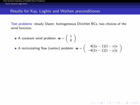
Test problems: steady Oseen, homogeneous Dirichlet BCs, two choices of thewind function.
A constant wind problem: w =
„10
«A recirculating flow (vortex) problem: w =
„4(2y − 1)(1− x)x−4(2x − 1)(1− y)y
«Uniform FEM discretizations: isoP2-P0 and isoP2-P1. These discretizationssatisfy the inf-sup condition: no pressure stabilization is needed.SUPG stabilization is used for the velocities.
The Krylov subspace method used is Bi-CGSTAB. This method requires twomatrix-vector multiplies with A and two applications of the preconditioner ateach iteration.
A preconditioning step requires two convection-diffusion solves (three in 3D)and one Poisson solve at each iteration, plus some mat-vecs.
Fast Iterative Solution of Saddle Point Problems
Some solution algorithms
Results for Kay, Loghin and Wathen preconditioner
Test problems: steady Oseen, homogeneous Dirichlet BCs, two choices of thewind function.
A constant wind problem: w =
„10
«
A recirculating flow (vortex) problem: w =
„4(2y − 1)(1− x)x−4(2x − 1)(1− y)y
«Uniform FEM discretizations: isoP2-P0 and isoP2-P1. These discretizationssatisfy the inf-sup condition: no pressure stabilization is needed.SUPG stabilization is used for the velocities.
The Krylov subspace method used is Bi-CGSTAB. This method requires twomatrix-vector multiplies with A and two applications of the preconditioner ateach iteration.
A preconditioning step requires two convection-diffusion solves (three in 3D)and one Poisson solve at each iteration, plus some mat-vecs.
Fast Iterative Solution of Saddle Point Problems
Some solution algorithms
Results for Kay, Loghin and Wathen preconditioner
Test problems: steady Oseen, homogeneous Dirichlet BCs, two choices of thewind function.
A constant wind problem: w =
„10
«A recirculating flow (vortex) problem: w =
„4(2y − 1)(1− x)x−4(2x − 1)(1− y)y
«
Uniform FEM discretizations: isoP2-P0 and isoP2-P1. These discretizationssatisfy the inf-sup condition: no pressure stabilization is needed.SUPG stabilization is used for the velocities.
The Krylov subspace method used is Bi-CGSTAB. This method requires twomatrix-vector multiplies with A and two applications of the preconditioner ateach iteration.
A preconditioning step requires two convection-diffusion solves (three in 3D)and one Poisson solve at each iteration, plus some mat-vecs.
Fast Iterative Solution of Saddle Point Problems
Some solution algorithms
Results for Kay, Loghin and Wathen preconditioner
Test problems: steady Oseen, homogeneous Dirichlet BCs, two choices of thewind function.
A constant wind problem: w =
„10
«A recirculating flow (vortex) problem: w =
„4(2y − 1)(1− x)x−4(2x − 1)(1− y)y
«Uniform FEM discretizations: isoP2-P0 and isoP2-P1. These discretizationssatisfy the inf-sup condition: no pressure stabilization is needed.SUPG stabilization is used for the velocities.
The Krylov subspace method used is Bi-CGSTAB. This method requires twomatrix-vector multiplies with A and two applications of the preconditioner ateach iteration.
A preconditioning step requires two convection-diffusion solves (three in 3D)and one Poisson solve at each iteration, plus some mat-vecs.
Fast Iterative Solution of Saddle Point Problems
Some solution algorithms
Results for Kay, Loghin and Wathen preconditioner
Test problems: steady Oseen, homogeneous Dirichlet BCs, two choices of thewind function.
A constant wind problem: w =
„10
«A recirculating flow (vortex) problem: w =
„4(2y − 1)(1− x)x−4(2x − 1)(1− y)y
«Uniform FEM discretizations: isoP2-P0 and isoP2-P1. These discretizationssatisfy the inf-sup condition: no pressure stabilization is needed.SUPG stabilization is used for the velocities.
The Krylov subspace method used is Bi-CGSTAB. This method requires twomatrix-vector multiplies with A and two applications of the preconditioner ateach iteration.
A preconditioning step requires two convection-diffusion solves (three in 3D)and one Poisson solve at each iteration, plus some mat-vecs.
Fast Iterative Solution of Saddle Point Problems
Some solution algorithms
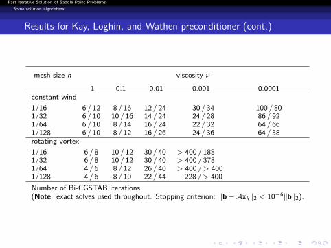
Results for Kay, Loghin, and Wathen preconditioner (cont.)
Number of Bi-CGSTAB iterations(Note: exact solves used throughout. Stopping criterion: ‖b−Axk‖2 < 10−6‖b‖2).
Fast Iterative Solution of Saddle Point Problems
The Augmented Lagrangian (AL) approach
Outline
Fast Iterative Solution of Saddle Point Problems
The Augmented Lagrangian (AL) approach
Augmented Lagrangian formulation of saddle point problems
Consider the equivalent augmented Lagrangian formulation (Fortin, Glowinski,1982) given by„
A + γBT W−1B BT
B O
«„up
«=
„f + γBT W−1g
g
«, (3)
where γ > 0 and W is symmetric positive definite.
Letting Aγ := A + γBT W−1B and fγ := f + γBT W−1g ,„Aγ BT
B O
«„up
«=
„fγg
«, or bA x = b. (4)
B. and Olshanskii introduced the following block preconditioner for (4)
P =
„Aγ BT
O bS«, bS−1 = −ν bM−1
p − γW−1. (5)
Fast Iterative Solution of Saddle Point Problems
The Augmented Lagrangian (AL) approach
Augmented Lagrangian formulation of saddle point problems
Consider the equivalent augmented Lagrangian formulation (Fortin, Glowinski,1982) given by„
A + γBT W−1B BT
B O
«„up
«=
„f + γBT W−1g
g
«, (3)
where γ > 0 and W is symmetric positive definite.Letting Aγ := A + γBT W−1B and fγ := f + γBT W−1g ,„
Aγ BT
B O
«„up
«=
„fγg
«, or bA x = b. (4)
B. and Olshanskii introduced the following block preconditioner for (4)
P =
„Aγ BT
O bS«, bS−1 = −ν bM−1
p − γW−1. (5)
Fast Iterative Solution of Saddle Point Problems
The Augmented Lagrangian (AL) approach
Analysis for the Oseen problem
Theorem (B./Olshanskii, SISC 2006)
Setting W = Mp, the preconditioned matrix P−1 bA has the eigenvalue 1 ofmultiplicity n; the remaining m eigenvalues are contained in a rectangle in theright half plane with sides independent of the mesh size h, and bounded awayfrom 0. Moreover, for γ = O(ν−1) the rectangle does not depend on ν. Whenγ →∞, all the eigenvalues tend to 1.
1
-1ε > 0
b
≈ 2
Re(λ)
Im(λ)
Fast Iterative Solution of Saddle Point Problems
The Augmented Lagrangian (AL) approach
Analysis for the Oseen problem (cont.)
Using field of values analysis, we can prove the following strongerparameter-independent convergence result for preconditioned GMRES:
Theorem (B./Olshanskii, SINUM 2011)
For ν < 1, if γ = ‖(BA−1BT )−1Mp‖Mp the residual norms in GMRES with theoriginal AL preconditioner satisfy
‖b− bAxk‖ ≤ qk‖b− bAx0‖,
where q < 1 is independent of problem parameters h, ν and α.
Recall that the field of values of an n× n matrix B is the subset of C defined by
F(B) := x∗Bx | x ∈ Cn, x∗x = 1 .
We proved that F(P−1A) is bounded and bounded away from 0 for all h, νand α. This implies the above convergence result for GMRES.
Fast Iterative Solution of Saddle Point Problems
The Augmented Lagrangian (AL) approach
Practical considerations
Applying P−1 to a vector requires one solve with Aγ and one with bS .
In practice we use W = bMp = diag(Mp)
The solve with Aγ can be approximated by a suitable geometric multigridmethod for elliptic systems (similar to the one by Schoberl, NM 1999)
For bS−1, a few Richardson iterations preconditioned with the diagonal ofMp can be used to solve the linear system with Mp.
Though the previous theorems suggest that γ = O(ν−1), in practice, γ = O(1)is sufficient for (near) parameter-independent convergence.
The rate of convergence of Krylov subspace method with this preconditioner isnearly optimal:
Independent of the grid; almost independent of viscosity
Cost is O(n + m) per iteration
Similar results with isoP2-P1 FEM
Fast Iterative Solution of Saddle Point Problems
The modified Augmented Lagrangian-based preconditioner
Outline
Fast Iterative Solution of Saddle Point Problems
The modified Augmented Lagrangian-based preconditioner
The modified augmented Lagrangian-based preconditioner
Motivation: Circumvent sophisticated geometric multigrid techniques in A−1γ ,
so as to be able to handle unstructured grids and more complex geometries.
From A = diag(A1,A2) and B = (B1,B2), we find
Aγ = A+γBT W−1B =
„A1 + γBT
1 W−1B1 γBT1 W−1B2
γBT2 W−1B1 A2 + γBT
2 W−1B2
«:=
„A11 A12
A21 A22
«.
The modified AL preconditioner (B., Olshanskii and Wang, IJNMF 2011) isdefined as
eP =
eAγ BT
O bS!
=
0@A11 A12 BT1
O A22 BT2
O O bS1A (6)
Aii = Ai + γBTi W−1Bi (i = 1, 2) can be interpreted as discrete scalar
anisotropic convection-diffusion operators with anisotropy ratio ≈ 1 + γν
.
They can be solved with standard algebraic multigrid (AMG) methods, inparticular, parallel AMG solvers.
Fast Iterative Solution of Saddle Point Problems
The modified Augmented Lagrangian-based preconditioner
The modified augmented Lagrangian-based preconditioner
Motivation: Circumvent sophisticated geometric multigrid techniques in A−1γ ,
so as to be able to handle unstructured grids and more complex geometries.From A = diag(A1,A2) and B = (B1,B2), we find
Aγ = A+γBT W−1B =
„A1 + γBT
1 W−1B1 γBT1 W−1B2
γBT2 W−1B1 A2 + γBT
2 W−1B2
«:=
„A11 A12
A21 A22
«.
The modified AL preconditioner (B., Olshanskii and Wang, IJNMF 2011) isdefined as
eP =
eAγ BT
O bS!
=
0@A11 A12 BT1
O A22 BT2
O O bS1A (6)
Aii = Ai + γBTi W−1Bi (i = 1, 2) can be interpreted as discrete scalar
anisotropic convection-diffusion operators with anisotropy ratio ≈ 1 + γν
.
They can be solved with standard algebraic multigrid (AMG) methods, inparticular, parallel AMG solvers.
Fast Iterative Solution of Saddle Point Problems
The modified Augmented Lagrangian-based preconditioner
Analysis
Note that
bA eP−1 =
0@ In/2 O O∗ In/2 − D E∗ F Im − G
1A .
The eigenvalues of bA eP−1 are λ = 1 of multiplicity n/2, plus the eigenvalues of„In/2 − D E
F Im − G
«= In/2+m −
„D −E−F G
«.
In general, the multiplicity of λ = 1 is only n/2.
However, letting bS−1 = −γW−1, the matrix on the right-hand side is rankdeficient by n/2, so bA eP−1 has the eigenvalue λ = 1 of multiplicity at least n.
Using field of values analysis, we can prove that the convergence rate ofGMRES with the modified AL preconditioner is h-independent, with amoderate dependence on ν.
Fast Iterative Solution of Saddle Point Problems
The modified Augmented Lagrangian-based preconditioner
The choice of γ
The value of the augmentation parameter γ is determined by local Fourieranalysis (LFA):
1 ‘discretize’ the diffusion and (frozen) convection terms in A by centereddifferences, assuming periodic BCs;
2 ‘discretize’ the gradient and divergence by one-sided differences;
3 note that W = bMp scales as h2;
4 express eP and bA in terms of “Fourier eigenvalues”, and find the γ thatminimizes the average distance of the non-unit eigenvalues λ(γ) of the
preconditioned matrix bA eP−1 from 1.
Note that γ only depends on h and ν. Hence it can be pre-computed, so nooverhead is imposed. The discretizations are symbolic.
Details in B. and Wang (SISC, 2011).
Fast Iterative Solution of Saddle Point Problems
The modified Augmented Lagrangian-based preconditioner
Example: a regularized lid driven cavity problem
All 2D experiments are done using IFISS package (Elman, Silvester & Ramage).
In the lid driven cavity problem, the flow is enclosed in a square withu1 = 1− x4, u2 = 0 on the top to represent the moving lid.
The modified Augmented Lagrangian-based preconditioner
Eigenvalues of preconditioned matrices
0 0.2 0.4 0.6 0.8 1
−0.3
−0.2
−0.1
0
0.1
0.2
0.3
0 0.2 0.4 0.6 0.8 1
−0.3
−0.2
−0.1
0
0.1
0.2
0.3
Figure: Plots of the eigenvalues of the preconditioned Oseen matrix (lid driven cavity,Q2-Q1, 32× 32 uniform grid, ν = 0.01). Left: with optimal γ. Right: with γ chosenby Fourier analysis.
The two values of γ are very close: 0.050 vs. 0.056.
The eigenvalue λ = 1 has multiplicity n (for all γ).
Fast Iterative Solution of Saddle Point Problems
The modified Augmented Lagrangian-based preconditioner
Iteration counts with various values of γ
Figure: GMRES iterations with modified AL preconditioner (cavity, Q2-Q1, uniformgrids, ν = 0.001)
0 0.02 0.04 0.06 0.08 0.120
25
30
35
40
45
50
55
60
Parameter γ
GM
RE
S it
erat
ions
64 × 64128 × 128
Fast Iterative Solution of Saddle Point Problems
The modified Augmented Lagrangian-based preconditioner
Iteration counts with Newton linearization
Use the same values of γ as for Picard linearization.
Table: GMRES iterations with modified AL preconditioner (cavity, Q2-Q1, stretchedgrids, Newton)
The modified Augmented Lagrangian-based preconditioner
Comparison of exact and inexact solves
In the following Table we present a comparison of modified AL preconditioningwith exact and inexact inversion of diagonal blocks Aii .
For the ‘exact’ solves we use the sparse LU factorization with column AMDreordering available in Matlab.
For the inexact solves we use one iteration (V-cycle) of AMG using theHSL−MI20 code developed by Boyle, Mihajlovic and Scott (IJNME 2010).
We perform tests for both Picard and Newton linearizations of the lid drivencavity problem discretized with Q2-Q1 elements (Newton is harder), using thesame value of γ from Fourier analysis in both cases. The viscosity is ν = 0.005.
The experiments are performed in Matlab 7.9.0 on a Sun Microsystems SunFire.
The upshot:
Using inexact solves does not affect the convergence rates
Inexact solves result in much faster solution times
Fast Iterative Solution of Saddle Point Problems
The modified Augmented Lagrangian-based preconditioner
Iteration counts and timings of exact solve and AMG (MI20)
Table: Comparison of exact and inexact inner solvers. GMRES iterations and timingswith modified AL preconditioner (cavity, Q2-Q1, uniform grids, ν = 0.005)
Set-up time 1.93 0.31 1.95 0.26Iter time 0.62 2.76 1.75 5.76
Total time 2.55 3.07 3.70 6.02128× 128 13 13 39 39Setup time 34.90 1.29 34.34 1.25
Iter time 4.44 12.00 10.94 29.38Total time 39.34 13.29 45.28 30.63256× 256 13 13 43 43Setup time 856.74 5.86 673.29 6.07
Iter time 40.22 58.84 85.84 152.05Total time 896.96 64.70 759.12 158.12
Fast Iterative Solution of Saddle Point Problems
The modified Augmented Lagrangian-based preconditioner
The modified AL preconditioner for 3D problems
For 3D Oseen problems A = diag(A1,A2,A3) and B = (B1,B2,B3).
Aγ = A + γBT W−1B
=
0@A1 O OO A2 OO O A3
1A+ γ
0@BT1
BT2
BT3
1AW−1 `B1 B2 B3
´
=
0@A1 + γBT1 W−1B1 γBT
1 W−1B2 γBT1 W−1B3
γBT2 W−1B1 A2 + γBT
2 W−1B2 γBT2 W−1B3
γBT3 W−1B1 γBT
3 W−1B2 A3 + γBT3 W−1B3
1A=:
0@A11 A12 A13
A21 A22 A23
A31 A32 A33
1A ,
so the modified AL preconditioner is
eP =
eAγ BT
O bS!
=
0BB@A11 A12 A13 BT
1
O A22 A23 BT2
O O A33 BT3
O O O bS1CCA .
Fast Iterative Solution of Saddle Point Problems
The modified Augmented Lagrangian-based preconditioner
Preliminary parallel results
These preliminary runs are done on a cluster having 32 nodes and 128 coresusing the Trilinos package (SNL). The subproblems in the modified ALpreconditioner are solved inexactly by one AMG iteration (‘ML’ solver inTrilinos). Each node of the cluster has two dual core AMD 2.2 GHz OpteronCPUs, 4 GB RAM and and 80 GB drive. The code is compiled and run withOpen MPI.
Steady 2D Oseen problem for the lid driven cavity (ν = 0.01), with γ chosen byFourier analysis. Q2-Q1 elements, 256× 256 grid.
Setup time 5.72 2.91 1.57 0.90 0.77 0.44Iter time 6.07 2.95 1.55 0.78 0.64 0.31
Total time 11.79 5.86 3.12 1.68 1.41 0.75
Fast Iterative Solution of Saddle Point Problems
The modified Augmented Lagrangian-based preconditioner
Preliminary parallel results
These preliminary runs are done on a cluster having 32 nodes and 128 coresusing the Trilinos package (SNL). The subproblems in the modified ALpreconditioner are solved inexactly by one AMG iteration (‘ML’ solver inTrilinos). Each node of the cluster has two dual core AMD 2.2 GHz OpteronCPUs, 4 GB RAM and and 80 GB drive. The code is compiled and run withOpen MPI.
Steady 2D Oseen problem for the lid driven cavity (ν = 0.01), with γ chosen byFourier analysis. Q2-Q1 elements, 256× 256 grid.
Iter time 67.88 29.24 25.41 12.88 8.11 4.33Total time 105.59 45.77 43.50 22.26 14.38 8.33
Fast Iterative Solution of Saddle Point Problems
Conclusions
Outline
Fast Iterative Solution of Saddle Point Problems
Conclusions
Conclusions and future work
Large linear systems of saddle point type still pose a significant challengefor modern preconditioned iterative solvers
Computing steady solutions to incompressible flow problems for smallvalues of the viscosity and on stretched grids is not easy
Suitably modified and combined with AMG-type inner solvers, the ALapproach results in fairly robust preconditioners
Both stable and stabilized discretizations can be accommodated
Stretched grids do not pose any difficulties to the AL approach
The Fourier-based approach gives very good estimates of the optimalparameter γ
Clearly better than competing methods on difficult problems
Current and future work: parallelization; application to real problems.
Fast Iterative Solution of Saddle Point Problems
Conclusions
References
1 M. Benzi and M. A. Olshanskii, Field-of-values analysis of augmented Lagrangianpreconditioners for the linearized Navier–Stokes problem, SIAM J. Numer. Anal.,49 (2011), pp. 770–788.
2 M. Benzi and Z. Wang, Analysis of augmented Lagrangian-based preconditionersfor the steady incompressible Navier–Stokes equations, SIAM J. Sci. Comput., 33(2011), pp. 2761–2784.
3 M. Benzi, M. A. Olshanskii and Z. Wang, Modified augmented Lagrangianpreconditioners for the incompressible Navier–Stokes equations, Intern. J.Numer. Meth. Fluids, 66 (2011), pp. 6185–6202.
4 M. Benzi and M. A. Olshanskii, An augmented Lagrangian-based approach tothe Oseen problem, SIAM J. Sci. Comput., 28 (2006), pp. 2095–2113.
5 K. A. Mardal and R. Winther, Preconditioning discretizations of systems ofpartial differential equations, Numer. Linear Algebra Appl., 18 (2011), pp. 1–40.
6 H. C. Elman, D. J. Silvester and A. J. Wathen, Finite Elements and FastIterative Solvers: With Applications in Incompressible Fluid Dynamics, OxfordUniversity Press, 2005.