Fast Marching Level Setstheory & applications

Mikkel B. Stegmann

04351 Advanced Image Analysis

IMM April 4th 2001

Introduction

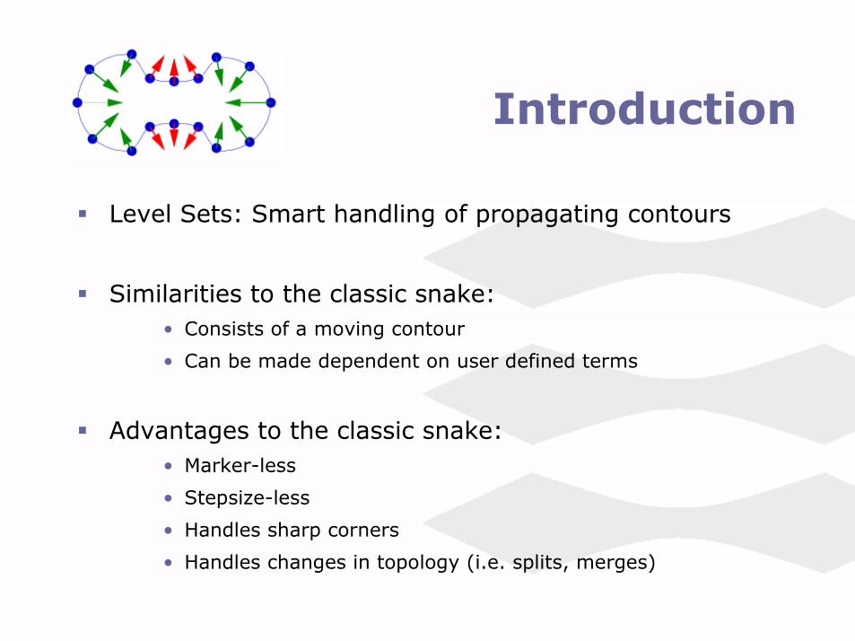
� Level Sets: Smart handling of propagating contours

� Similarities to the classic snake:• Consists of a moving contour

• Can be made dependent on user defined terms

� Advantages to the classic snake:• Marker-less

• Stepsize-less

• Handles sharp corners

• Handles changes in topology (i.e. splits, merges)

Consequences of marker-based evolution

� Example: Propagation of two flames

Initial

Later Later (marker-based solution)

A level set representation

� Adding an extra dimension to the problem

The level set function:

z = ΦΦΦΦ(x,y,t)

Contour at time t:

0 = ΦΦΦΦ(x,y,t)

The level set PDE:

ΦΦΦΦt + F|∇ΦΦΦΦ| = 0

given ΦΦΦΦ(x,y,t=0)

Fast marching

� Observations• If F preserves sign, then the level set function

ΦΦΦΦ(x,y,t) = 0 becomes single-valued in t, i.e. each pixel is visited once

• This leads to the simpler Eikonal equation formulation

|∇u(x,y)|F = 1

where u is the arrival time of the front

• Combined with an optimal sorting technique, this leads to a very fast solution to ΦΦΦΦ(x,y,t=t0) = 0

F = 1

u = 4

u = 0

Propagation of concave contours

� The swallowtail problem� Imagine the propagation of a concave contour with F = 1

� Adding viscosity in terms of curvature, leads to a simple curve, but the solution is somewhat smoothed

� However, using Huygen’s Principle the front should produce a sharp corner (which is no good in a PDE formulation)

� A solution

� Let ε → 0 or integrate the viscosity solution (or weak solution) into the numerical approximation of the gradient

Swallowtail, F = 1 Front propagating with viscosity, F = 1 + εκ

Huygen’s Principle: ”Every point on a primary wave front serves as the source of spherical secondary wavelets such that the primary wave front at some later time is the envelope of these wavelets...”

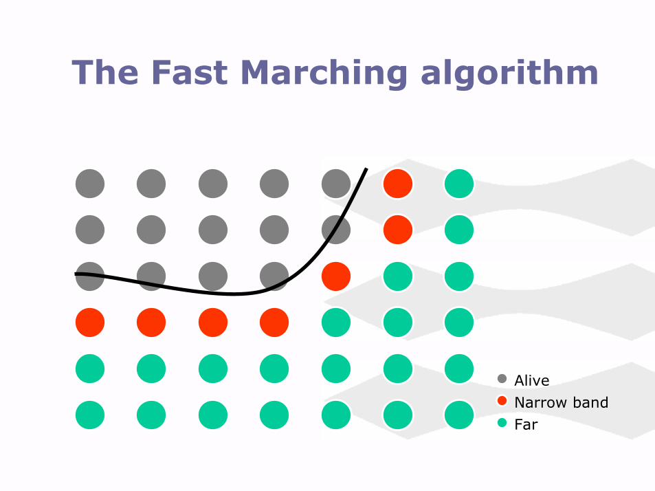
The Fast Marching algorithm

AliveNarrow bandFar

The Fast Marching algorithm

� Loop {

1. Let Trial be the point in Narrow band with smallest u

2. Move Trial from Narrow band to Alive

3. Move all neighbors of Trial to Narrow band

4. Recompute u for all neighbors of Trial

}

AliveNarrow bandFar

Fast marching – cont’d

(1) (2) (3)

(4) (5) (6)

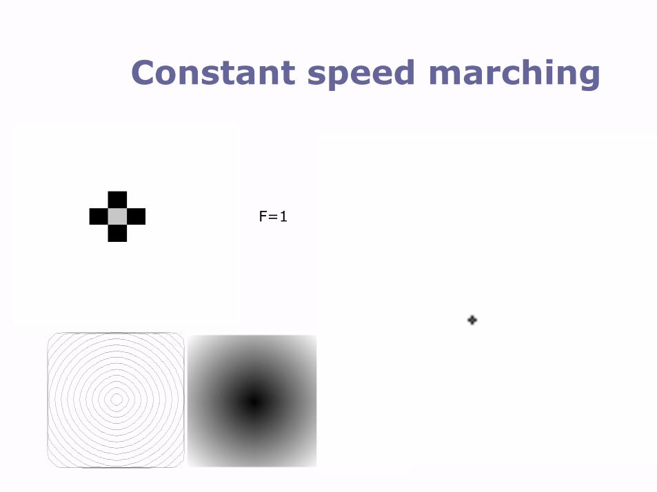
Constant speed marching

F=1

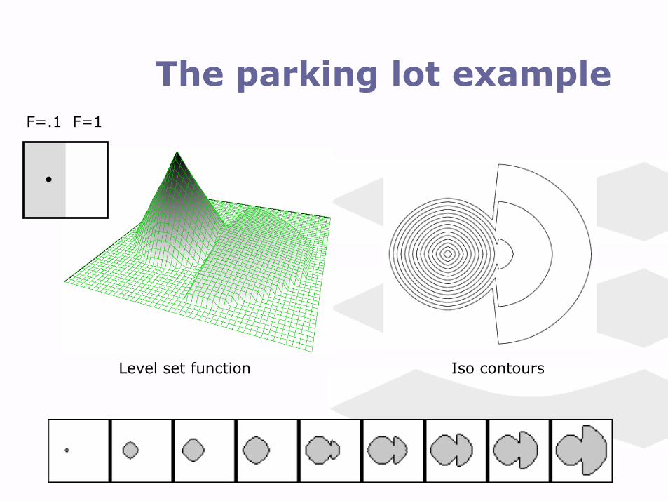
The parking lot exampleF=.1 F=1

Level set function Iso contours

Fast marching in details

� How to: ”4) Recompute u for all neighbors of Trial”

• That is: solve the Eikonal eq. |∇u|F = 1 at all neighbors

• The correct viscosity solution is obtained by:

max( max(ux,y – ux-1,y,0), -min(ux+1,y – ux,y,0) )2 + max( max(ux,y – ux,y-1,0), -min(ux,y+1 – ux,y,0) )2 = 1/F2

• Example:

(ux,y – ux+1,y)2+(ux,y – ux,y-1)2 = 1/F2

y-1

x-1 x+1

y+1

ux,y

Fast marching in details

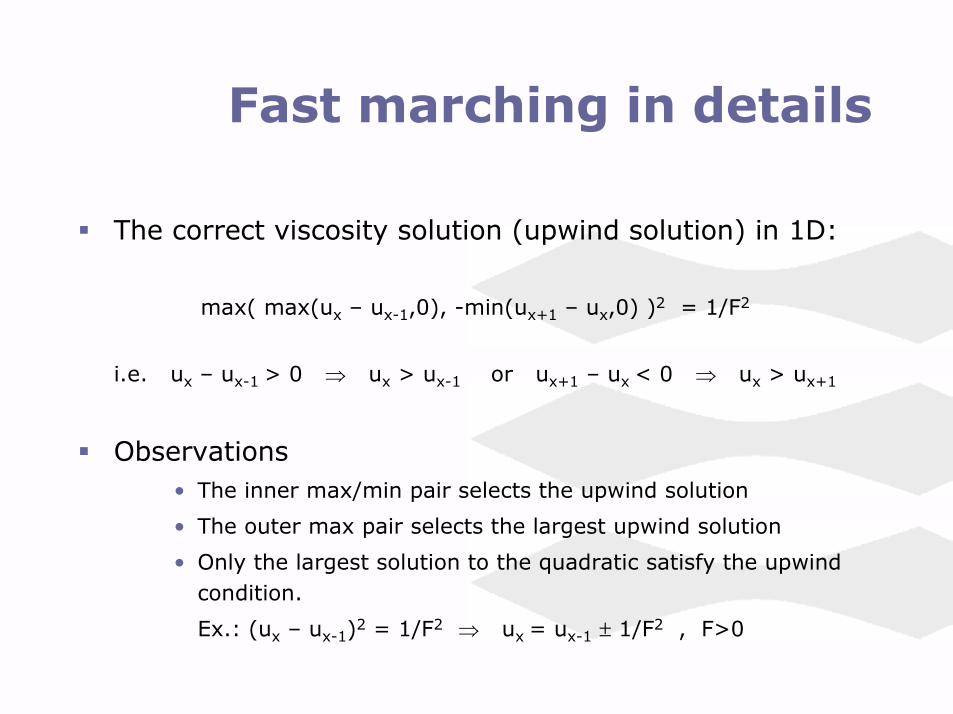
� The correct viscosity solution (upwind solution) in 1D:

max( max(ux – ux-1,0), -min(ux+1 – ux,0) )2 = 1/F2

i.e. ux – ux-1 > 0 ⇒ ux > ux-1 or ux+1 – ux < 0 ⇒ ux > ux+1

� Observations• The inner max/min pair selects the upwind solution

• The outer max pair selects the largest upwind solution

• Only the largest solution to the quadratic satisfy the upwind condition.

Ex.: (ux – ux-1)2 = 1/F2 ⇒ ux = ux-1 ± 1/F2 , F>0

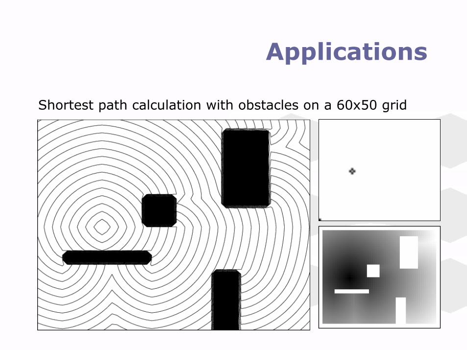
Applications

Shortest path calculation with obstacles on a 60x50 grid

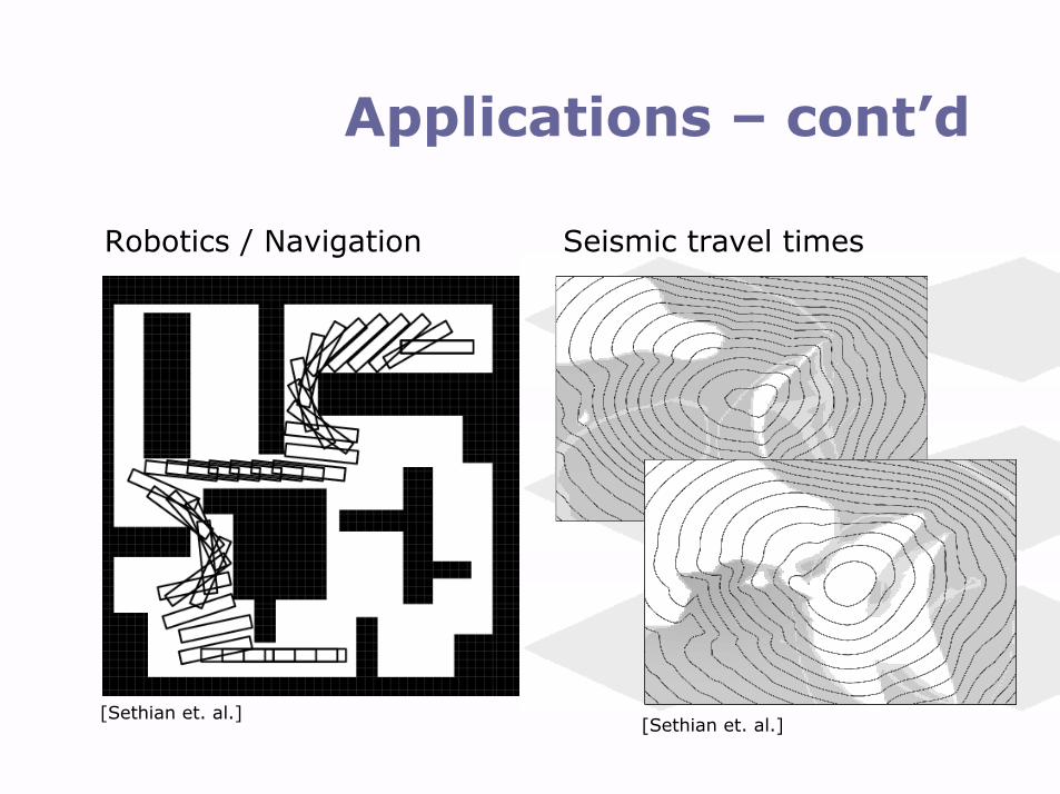
Applications – cont’d

Robotics / Navigation Seismic travel times

[Sethian et. al.][Sethian et. al.]

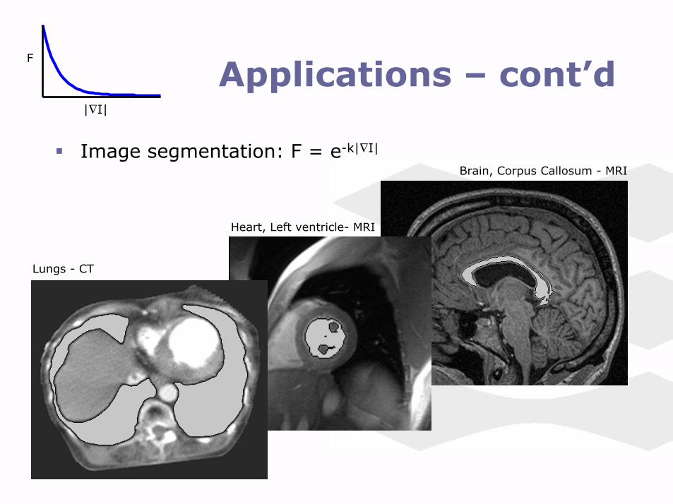
Applications – cont’d

� Image segmentation: F = e-k|∇I|

Lungs - CT

Heart, Left ventricle- MRI

Brain, Corpus Callosum - MRI

|∇I|

F

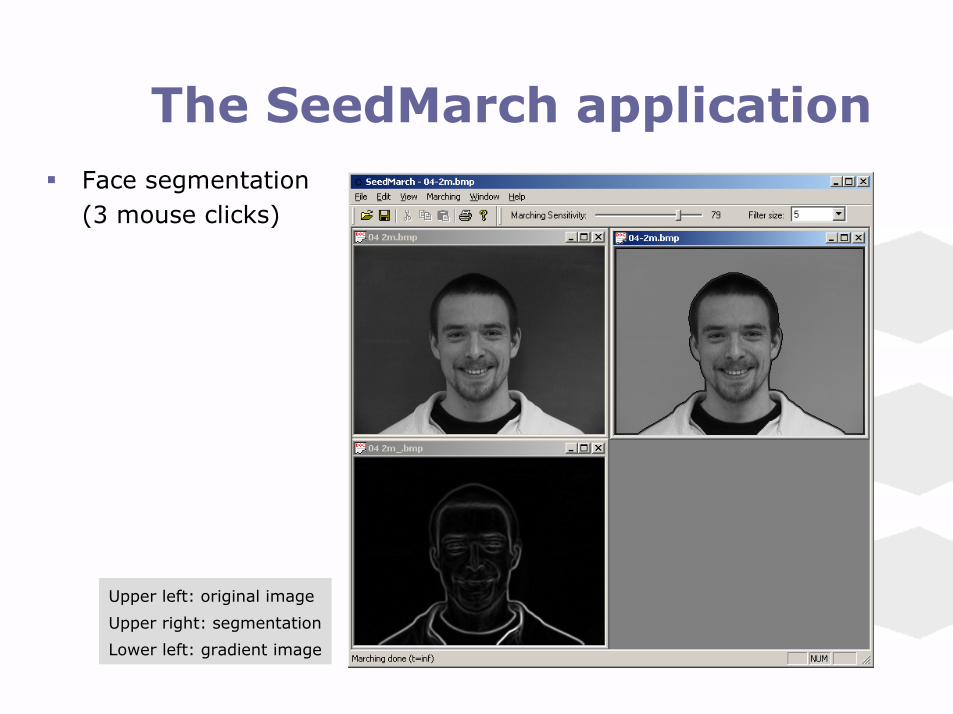
The SeedMarch application� Face segmentation

(3 mouse clicks)

Upper left: original image

Upper right: segmentation

Lower left: gradient image

Summary

� Fast Marching methods are:• Very efficient – also in 3D

• Of an ’open architecture’ in terms of speed functions

• Dealing with sharp corners and changes in topology

• Widely applicable: image segmentation, robotics, seismic travel times, shortest path finding etc.

• In essence a smart way to solve the Eikonal equation

� Discussion• Can inherently only propagate monotonically

• The more general – but slower – level set formulation handles non-monotonically advancing fronts

• Stop criteria selection is crucial w.r.t. image segmentation

Project proposal I

� A 3D Fast Marching Implementation

[Bærentzen]

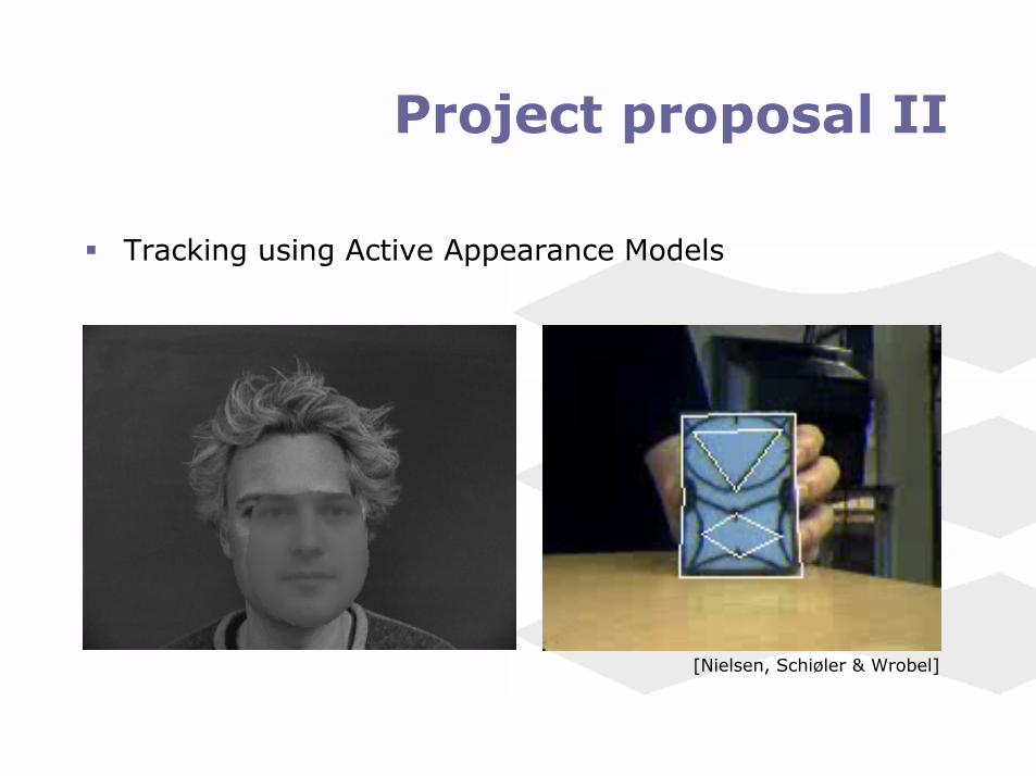
Project proposal II

� Tracking using Active Appearance Models

[Nielsen, Schiøler & Wrobel]

The End

� Acknowledgements

• M.Sc., Ph.D. Stud. Andreas Bærentzen, IMM

• Selected illustrations from publications of J.A. Sethian

� References

• J.A. Sethian, ”Level Set Methods and Fast Marching Methods”, Cambridge University Press, 1999

• http://www.math.berkeley.edu/~sethian/