Fast Methods for Scheduling with Applications to Real-Time Systems and Large-Scale, Robotic Manufacturing of Aerospace Structures by Matthew C. Gombolay Submitted to the Department of Aeronautics and Astronautics in partial fulfillment of the requirements for the degree of Master of Science in Aeronautics and Astronautics at the MASSACHUSETTS INSTITUTE OF TECHNOLOGY June 2013 c Massachusetts Institute of Technology 2013. All rights reserved. Author .............................................................. Department of Aeronautics and Astronautics June 7, 2013 Certified by .......................................................... Julie A. Shah Assistant Professor of Aeronautics and Astronautics Thesis Supervisor Accepted by ......................................................... Eytan H. Modiano Professor of Aeronautics and Astronautics Chair, Graduate Program Committee
Transcript
Fast Methods for Scheduling with Applications to
Real-Time Systems and Large-Scale, Robotic
Manufacturing of Aerospace Structures
by
Matthew C. Gombolay
Submitted to the Department of Aeronautics and Astronauticsin partial fulfillment of the requirements for the degree of
Professor of Aeronautics and AstronauticsChair, Graduate Program Committee
2
Fast Methods for Scheduling with Applications to Real-Time
Systems and Large-Scale, Robotic Manufacturing of
Aerospace Structures
by
Matthew C. Gombolay
Submitted to the Department of Aeronautics and Astronauticson June 7, 2013, in partial fulfillment of the
requirements for the degree ofMaster of Science in Aeronautics and Astronautics
Abstract
Across the aerospace and automotive manufacturing industries, there is a push toremove the cage around large, industrial robots and integrate right-sized, safe versionsinto the human labor force. By integrating robots into the labor force, humans canbe freed to focus on value-added tasks (e.g. dexterous assembly) while the robotsperform the non-value-added tasks (e.g. fetching parts). For this integration to besuccessful, the robots need to ability to reschedule their tasks online in response tounanticipated changes in the parameters of the manufacturing process.
The problem of task allocation and scheduling is NP-Hard. To achieve good scala-bility characteristics, prior approaches to autonomous task allocation and schedulinguse decomposition and distributed techniques. These methods work well for domainssuch as UAV scheduling when the temporospatial constraints can be decoupled orwhen low network bandwidth makes inter-agent communication difficult. However,the advantages of these methods are mitigated in the factory setting where the tem-porospatial constraints are tightly inter-coupled from the humans and robots workingin close proximity and where there is sufficient network bandwidth.
In this thesis, I present a system, called Tercio, that solves large-scale schedul-ing problems by combining mixed-integer linear programming to perform the agentallocation and a real-time scheduling simulation to sequence the task set. Tercio gen-erates near optimal schedules for 10 agents and 500 work packages in less than 20seconds on average and has been demonstrated in a multi-robot hardware test bed.My primary technical contributions are fast, near-optimal, real-time systems meth-ods for scheduling and testing the schedulability of task sets. I also present a pilotstudy that investigates what level of control the Tercio should give human workersover their robotic teammates to maximize system efficiency and human satisfaction.
Thesis Supervisor: Julie A. ShahTitle: Assistant Professor of Aeronautics and Astronautics
3
4
Acknowledgments
Personal Acknowledgments
Over the past two years, I have had the unwavering support of a number of individuals
and groups that I would like to personally thank. Assistant Professor Julie Shah, my
advisor and mentor has inspired me, constructively criticized my work, and helped
to form me into a capable researcher. I thank her for her energetic support. Further,
I want to thank Professor Julie Shah’s Interactive Robotics Group (IRG) for their
support in my research as peer-reviewers, test subjects, and friends.
My family has been a constant support for my entire life. My parents, Craig and
Lauren, sister, Alli, and Grandparents, Fred and Vivan, have given me the love and
support necessary for me to reach my goals. I treasure their support. I also want
to thank Grace, who has been my comfort, companion, and best friend. Lastly, and
most importantly, I praise God for the breath he breathes in my lungs, that I might
bring the gospel of Jesus Christ to those who do not know Him.
Funding
Funding for this project was provided by Boeing Research and Technology and The
National Science Foundation (NSF) Graduate Research Fellowship Program (GRFP)
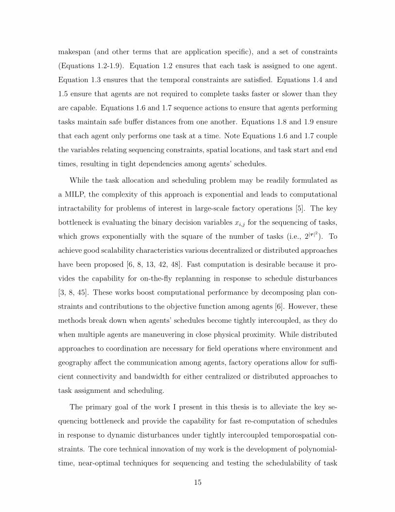
Robotic systems are increasingly entering domains previously occupied exclusively
by humans. In manufacturing, there is strong economic motivation to enable human
and robotic agents to work in concert to perform traditionally manual work. This
integration requires a choreography of human and robotic work that meets upper-
bound and lowerbound temporal deadlines on task completion (e.g. assigned work
must be completed within one shift) and spatial restrictions on agent proximity (e.g.
robots must maintain four meter separation from other agents) to support safe and
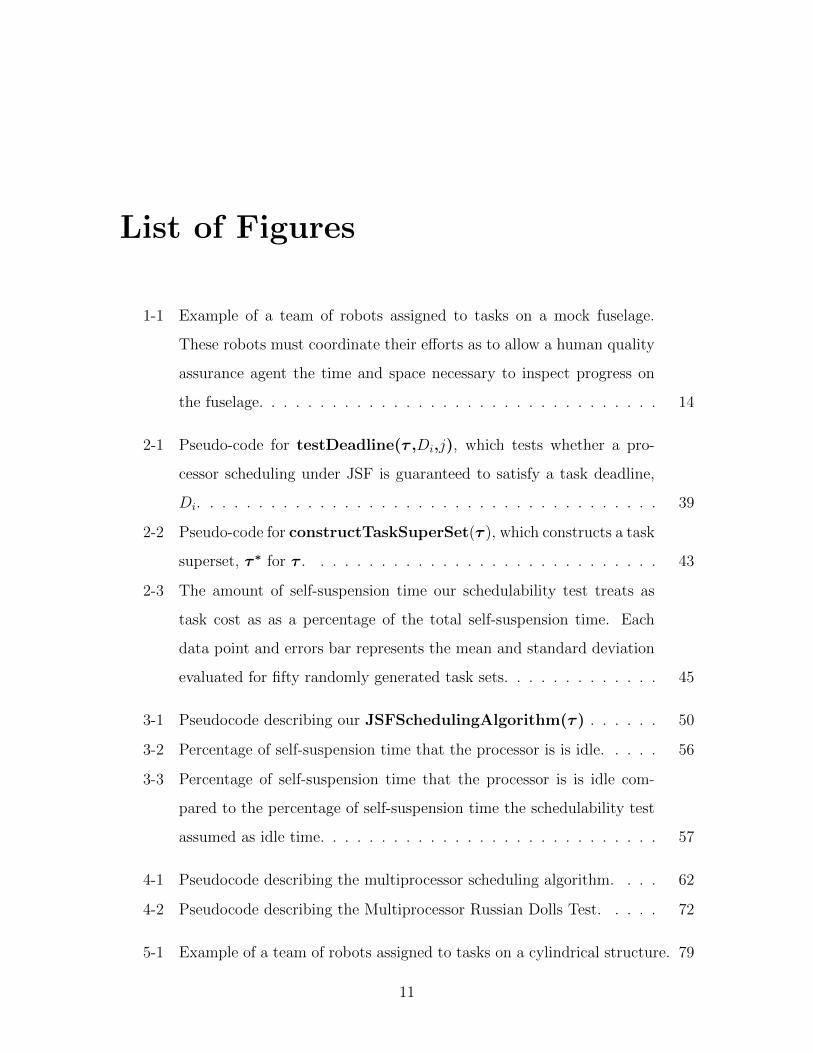
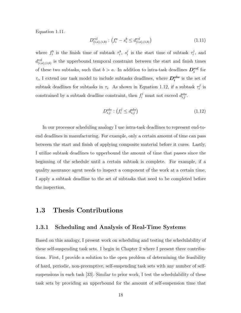
efficient human-robot co-work. Figure 1-1 shows an example scenario where a human
quality assurance agent must co-habit work space with robots without delaying the
manufacturing process. The multi-agent coordination problem with temporospatial
constraints can be readily formulated as a mixed-integer linear program (MILP).
1.1 Formal Problem Description
min(z), z = maxi,j
(fj − si) + g (x,A, s, f, τ ) (1.1)
subject to ∑a∈A
Aa,i = 1,∀i ∈ τ (1.2)
lbi,j ≤ fi − sj ≤ ubi,j,∀(i, j) ∈ γ (1.3)
13
Figure 1-1: Example of a team of robots assigned to tasks on a mock fuselage. Theserobots must coordinate their efforts as to allow a human quality assurance agent thetime and space necessary to inspect progress on the fuselage.
and subtask deadlines (i.e., Equation 1.12). The scheduling algorithm utilizes a
polynomial-time, online consistency test, which I call the Multiprocessor Russian
Dolls Test, to ensure temporal consistency due to the temporal and shared memory
resource constraints of the task set.
19
1.3.2 Tercio: a Task Allocation and Scheduling Algorithm
Based on the techniques I develop in the scheduling of these self-suspending task
sets in Chapters 2-4, I designed a multi-agent task allocation and scheduling system,
called Tercio1[22]. The algorithm is made efficient by decomposing task allocation
from scheduling and utilizes the techniques I present in Chapter 4 to perform multi-
agent sequencing. Results show that the method is able to generate near-optimal task
assignments and schedules for up to 10 agents and 500 tasks in less than 20 seconds on
average. In this regard, Tercio scales better than previous approaches to hybrid task
assignment and scheduling [9, 10, 25, 26, 27, 49]. Although the sequencing algorithm
is satisficing, I show that it is tight, meaning it produces near-optimal task sequences
for real-world, structured problems. An additional feature of Tercio is that it returns
flexible time windows for execution [38, 52], which enable the agents to adapt to small
disturbances online without a full re-computation of the schedule. I present this work
in Chapter 5.
1.3.3 Human-Centered Integration of Centralized Schedul-
ing Algorithms
While fast task assignment and scheduling is an important step to enabling the in-
tegration of robots into the manufacturing environment, we also need to consider a
human-centered approach when implementing Tercio in the factory. Successful in-
tegration of robot systems into human teams requires more than tasking algorithms
that are capable of adapting online to the dynamic environment. The mechanisms
for coordination must be valued and appreciated by the human workers. Human
workers often find identity and security in their roles or jobs in the factory and are
used to some autonomy in decision-making. A human worker that is instead tasked
by an automated scheduling algorithm may begin to feel that he or she is diminished.
Even if the algorithm increases process efficiency at first, there is concern that taking
control away from the human workers may alienate them and ultimately damage the
1Joint work with Ronald Wilcox
20
productivity of the human-robot team. The study of human factors can inform the
design of effective algorithms for collaborative tasking of humans and robots.
In Chapter 6, I describe a pilot study2 conducted to gain insight into how to inte-
grate multi-agent task allocation and scheduling algorithms to improve the efficiency
of coordinated human and robotic work[21]. In one experimental condition, both the
human and robot are tasked by Tercio, the automatic scheduling algorithm. In the
second condition, the human worker is provided with a limited set of task allocations
from which he/she can choose. I hypothesize that giving the human more control
over the decision-making process will increase worker satisfaction, but that doing
so will decrease system efficiency in terms of time to complete the task. Analysis
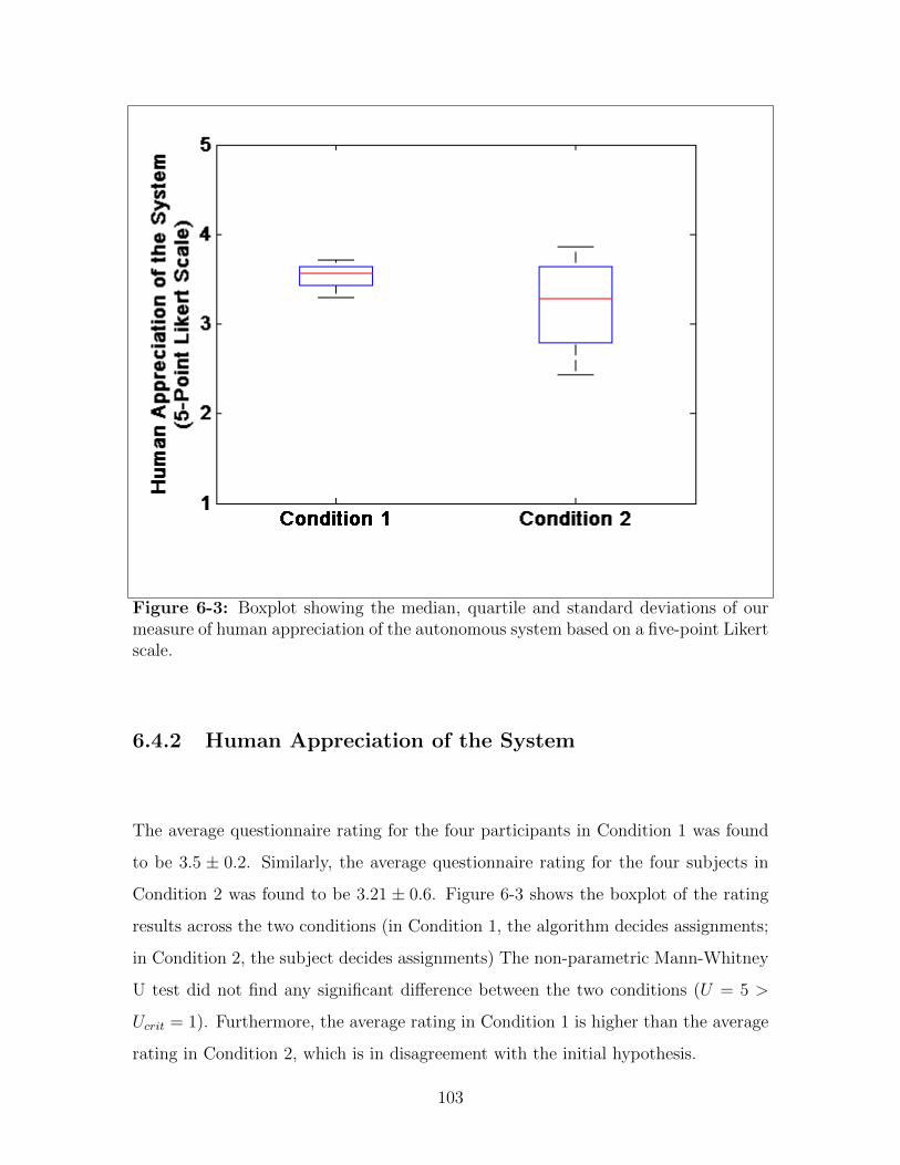
of the experimental data (n = 8) shows that when workers were given freedom to
choose, process efficiency decreased significantly. However, user-satisfaction seems
to be confounded by whether or not the subject chose the optimal task allocation.
Four subjects were allowed to choose their task allocation. Within that pool, the
one subject that chose the optimal allocation rated his/her satisfaction the highest
of all subjects tested, and the mean of the satisfaction rating of the three who chose
the suboptimal allocation was lower than those subjects who’s roles were assigned
autonomously.
2Joint work with Ronald Wilcox, Ana Diaz Artiles, and Fei Yu
21
22
Chapter 2
Uniprocessor Schedulability Test
for Hard, Non-Preemptive,
Self-Suspending Task Sets with
Multiple Self-Suspensions per Task
2.1 Introduction
In this chapter, we present three contributions. First, we provide a solution to the
open problem of determining the feasibility of hard, periodic, non-preemptive, self-
suspending task sets with any number of self-suspensions in each task [33]. Similar to
prior work, we test the schedulability of these task sets by providing an upperbound
for the amount of self-suspension time that needs to be treated as task cost [34, 35,
36, 44]. Our test is polynomial in time and, in contrast to prior art, generalizes to
non-preemptive task sets with more than one self-suspension per task.
Second, we extend our schedulability test to also handle task sets with deadlines
constraining the upperbound temporal difference between the start and finish of two
subtasks within the same task. Third, we introduce a new scheduling policy to
accompany the schedulability test. We specifically designed this scheduling policy to
23
restrict the behavior of a self-suspending task set so as to provide an analytical basis
for an informative schedulability test.
We begin in Section 2.2 with a brief review or prior work. In Section 2.3, we intro-
duce our augmented self-suspending task model. Next, we introduce new terminology
to help describe our schedulability test and the execution behavior of self-suspending
tasks in Section 2.4. We then motivate our new scheduling policy, which restricts
the behavior of the scheduler to reduce scheduling anomalies 2.5. In Section 2.6,
we present our schedulability test, with proof of correctness. Finally, in Section 2.7,
we empirically validate that the test is tight, meaning that it does not significantly
overestimate the temporal resources needed to execute the task set.
2.2 Background
Increasingly in real-time systems, computer processors must handle the self-suspension
of tasks and determine the feasibility of these task sets. Self-suspensions can result
both due to hardware and software architecture. At the hardware level, the addi-
tion of multi-core processors, dedicated cards (e.g., GPUs, PPUs, etc.), and various
I/O devices such as external memory drives, can necessitate task self-suspensions.
Furthermore, the software that utilizes these hardware systems can employ synchro-
nization points and other algorithmic techniques that also result in self-suspensions
[33]. Thus, a schedulability test that does not significantly overestimate the temporal
resources needed to execute self-suspending task sets would be of benefit to these
modern computing systems.
Unfortunately the problem is NP-Hard, as can be shown through an analysis
of the interaction of self-suspensions and task deadlines [24, 38]. In practice, the
relaxation of a deadline in a self-suspending task set may result in temporal infeasi-
bility. Many uniprocessor, priority-based scheduling algorithms introduce scheduling
anomalies since they do not account for this interaction [32, 44]. The most straight-
forward, correct approach for testing the schedulability of these task sets is to treat
self-suspensions as task costs; however, this can result in significant under-utilization
24
of the processor if the duration of self-suspensions is large relative to task costs [36, 37].
A number of different approaches have been proposed to test the schedulability
of self-suspending task sets. The dominant strategy is to upperbound the duration
of self-suspensions that needs to be treated as task cost [34, 36]. Recently, Liu and
Anderson et al. have demonstrated significant improvements over prior art in testing
preemptive task sets with multiple self-suspensions per task, under Global Earliest
Deadline First (GEDF) on multiple processor systems [36]. Previously, Devi proposed
a test to compute the maximum utilization factor for tasks with single self-suspensions
scheduled under Earliest Deadline First (EDF) for uniprocessor systems. The test
works by analyzing priorities to determine the number of tasks that may be executed
during a self-suspension [15]. Other approaches test schedulability by analyzing the
worst case response time of tasks due to external blocking events [24, 29, 50].
The design of scheduling policies for self-suspending task sets also remains a chal-
lenge. While EDF has desirable properties for many real-time uniprocessor scheduling
problems, certain anomalies arise when scheduling task sets with both self-suspensions
and hard deadlines. Ridouard et al. note an example where it is possible to schedule
a task set under EDF with tight deadlines, while the same task set with looser dead-
lines fails [44]. Lakshmanan et al. report that finding an anomaly-free scheduling
priority for self-suspending task sets remains an open problem [32].
While not anomaly-free, various priority-based scheduling policies have been shown
to improve the online execution behavior in practice. For example, Rajkumar presents
an algorithm called Period Enforcer that forces tasks to behave as ideal, periodic tasks
to improve scheduling performance and avoid detrimental scheduling anomalies asso-
ciated with scheduling unrestricted, self-suspending task sets [41]. Similarly, Sun et al.
presents a set of synchronization protocols and a complementary schedulability test
to determine the feasibility of a task set for a scheduler operating under the protocols
[47]. Lakshmanan builds on these approaches to develop a static slack enforcement
algorithm that delays the release times of subtasks to improve the schedulability of
task sets [33].
Similar to the approach of Lakshmanan et al., we develop a priority-based schedul-
25
ing algorithm that reduces anomalies in practice. This policy enables us analytically
upperbound the duration of the self-suspensions that needs to be treated as task cost,
similar to the approach by Liu et al.. To our knowledge, our schedulability test is
the first that determines the feasibility of hard, non-preemptive, self-suspending task
sets with multiple self-suspensions for each task.
2.3 Our Augmented Task Model
The basic model for self-suspending task sets is shown in Equation 2.1.
τi : (φi, (C1i , E
1i , C
2i , E
2i , . . . , E
mi−1
i , Cmii ), Ti, Di,D
reli ) (2.1)
In this model, there is a task set, τ , where all tasks, τi ∈ τ must be executed by
a uniprocessor. For each task, there are mi subtasks with mi − 1 self-suspension
intervals. Cji is the worst-case duration of the jth subtask of τi, and Ej
i is the worst-
case duration of the jth self-suspension interval of τi.
Subtasks within a task are dependent, meaning that a subtask τ j+1i must start
after the finish times of the subtask τ ji and the self-suspension Eji . Ti and Di are the
period and deadline of τi, respectively, where Di ≤ Ti. Lastly, a phase offset delays
the release of a task, τi, by the duration, φi, after the start of a new period.
In this work, we augment the traditional model to provide additional expressive-
ness, by incorporating deadline constraints that upperbound the temporal difference
between the start and finish of two subtasks within a task. We call these deadline con-
straints intra-task deadlines. We define an intra-task deadline as shown in Equation
2.2.
Drel(i,a),(i,b) :
(fai − sbi ≤ drel(i,a),(i,b)
)(2.2)
where f bi is the finish time of subtask τ bi , sji is the start time of subtask τ ji , and
drel(i,a),(i,b) is the upperbound temporal constraint between the start and finish times of
these two subtasks, such that b > a. Dreli is the set of intra-task deadlines for τi, and
Drel is the set of intra-task deadlines for τ . These types of constraints are commonly
26
included in AI and operations research scheduling models [5, 14, 38, 52].
2.4 Terminology
In this section we introduce new terminology to help describe our schedulability test
and the execution behavior of self-suspending tasks, which in turn will help us intu-
itively describe the various components of our schedulability test.
Definition 1. A free subtask, τ ji ∈ τfree, is a subtask that does not share a deadline
constraint with τ j−1i . In other words, a subtask τ ji is free iff for any deadline Drel(i,a)(i,b)
associated with that task, (j ≤ a)∨ (b < j). We define τ 1i as free since there does not
exist a preceding subtask.
Definition 2. An embedded subtask, τ j+1i ∈ τembedded, is a subtask shares a deadline
constraint with τ ji (i.e., τ j+1i /∈ τfree). τfree ∩ τembedded = ∅.
The intuitive difference between a free and an embedded subtask is as follows: a
scheduler has the flexibility to sequence a free subtask relative to the other free sub-
tasks without consideration of intra-task deadlines. On the other hand, the scheduler
must take extra consideration to satisfy intra-task deadlines when sequencing an em-
bedded subtask relative to other subtasks.
Definition 3. A free self-suspension, Eji ∈ Efree, is a self-suspension that suspends
two subtasks, τ ji and τ j+1i , where τ j+1
i ∈ τfree.
Definition 4. An embedded self-suspension, Eji ∈ Eembedded, is a self-suspension
that suspends the execution of two subtasks, τ ji and τ j+1i , where τ j+1
i ∈ τembedded.
Efree ∩Eembedded = ∅.
In Section 2.6, we describe how we can use τfree to reduce processor idle time due
to Efree, and, in turn, analytically upperbound the duration of the self-suspensions
that needs to be treated as task cost. We will also derive an upperbound on processor
idle time due to Eembedded.
27
2.5 Motivating our jth Subtask First (JSF) Prior-
ity Scheduling Policy
Scheduling of self-suspending task sets is challenging because polynomial-time, priority-
based approaches such as EDF can result in scheduling anomalies. To construct a
tight schedulability test, we desire a priority method of restricting the execution be-
havior of the task set in a way that allows us to analytically bound the contributions
of self-suspensions to processor idle time, without unnecessarily sacrificing processor
efficiency.
We restrict behavior using a novel scheduling priority, which we call jth Subtask
First (JSF). We formally define the jth Subtask First priority scheduling policy in
Definition 5.
Definition 5. jth Subtask First (JSF). We use j to correspond to the subtask index in
τ ji . A processor executing a set of self-suspending tasks under JSF must execute the jth
subtask ( free or embedded) of every task before any jth+1 free subtask. Furthermore,
a processor does not idle if there is an available free subtask unless executing that free
task results in temporal infeasibility due to an intra-task deadline constraint.
Enforcing that all jth subtasks are completed before any jth + 1 free subtasks
allows the processor to execute any embedded kth subtasks where k > j as necessary to
ensure that intra-task deadlines are satisfied. The JSF priority scheduling policy offers
choice among consistency checking algorithms. A simple algorithm to ensure deadlines
are satisfied would require that, if a free subtask that triggers a deadline constraint is
executed (i.e. τ ji ∈ τfree, τj+1i ∈ τembedded), the subsequent embedded tasks for the
associated deadline constraint would then be scheduled as early as possible without
the processor executing any other subtasks during this duration. Other consistency-
check algorithms exist that utilize processor time more efficiently and operate on this
structured task model [19, 31, 51].
28
2.6 Schedulability Test
To describe how our test works and prove its correctness, we will start with a simplified
version of the task set and build to the full task model. We follow the following six
steps:
1. We restrict τ such that each task only has two subtasks (i.e., mi = 2,∀i),
there are no intra-task deadlines, and all tasks are released at t = 0 (i.e.,
φ = 0,∀i). Here we will introduce our formula for upperbounding the amount
of self-suspension time that we treat as task cost, Wfree. Additionally, we say
that all tasks have the same period and deadline (i.e., Ti = Di = Tj = Dj,∀i, j ∈
{1, 2, . . . , n}). Thus, the hyperperiod of the task set is equal to the period of
each task.
2. Next, we allow for general task release times (i.e., φi ≥ 0,∀i). In this step, we
upperbound processor idle time due to phase offsets, Wφ.
3. Third, we relax the restriction that each task has two subtasks and say that
each task can have any number of subtasks.
4. Fourth, we incorporate intra-task deadlines. In this step, we will describe
how we calculate an upperbound on processor idle time due to embedded self-
suspensions Wembedded.
5. Fifth, we relax the uniform task deadline restriction and allow for general task
deadlines where Di ≤ Ti,∀i ∈ {1, 2, . . . , n}.
6. Lastly, we relax the uniform periodicity restriction and allow for general task
periods where Ti 6= Tj,∀i, j ∈ {1, 2, . . . , n}.
Step 1) Two Subtasks Per Task, No Deadlines, and Zero Phase
Offsets
In step one, we consider a task set, τ with two subtasks per each of the n tasks, no
intra-task deadlines, and zero phase offsets (i.e., φi = 0,∀i ∈ n). Furthermore, we say
29
that task deadlines are equal to task periods, and that all tasks have equal periods
(i.e., Ti = Di = Tj = Dj,∀i, j ∈ {1, 2, . . . , n}). We assert that one can upperbound
the idle time due to the set of all of the E1i self-suspensions by analyzing the difference
between the duration of the self-suspensions and the duration of the subtasks costs
that will be interleaved during the self-suspensions.
We say that the set of all subtasks that might be interleaved during a self-
suspension, E1i , is B1
i . As described by Equation 2.3, Bji is the set of all of the
jth and jth + 1 subtask costs less the subtasks costs for τ ji and τ j+1i . Note, by defini-
tion, τ ji and τ j+1i cannot execute during Ej
i . We further define an operator Bji (k) that
provides the kth smallest subtask cost from Bji . We also restrict Bj
i such that the jth
and jth + 1 subtasks must both be free subtasks if either is to be added. Because we
are currently considering task sets with no deadlines, this restriction does not affect
the subtasks in B1i during this step. In Step 4 (Section 2.6), we will explain why we
make this restriction on the subtasks in Bji .
For convenience in notation, we say that N is the set of all task indices (i.e., N =
{i|i ∈ {1, 2, . . . , n}}, where n is the number of tasks in the task set, τ ). Without loss of
generality, we assume that the first subtasks τ 1i execute in the order i = {1, 2, . . . , n}.
Bji = {Cy
x |x ∈ N\i, y ∈ {j, j + 1},
τ jx ∈ τfree, τ j+1x ∈ τfree}
(2.3)
To upperbound the idle time due to the set of E1i self-suspensions, we consider
a worst-case interleaving of subtask costs and self-suspension durations, as shown in
Equation 2.6 and Equation 2.5 where W ji is an upperbound on processor idle time
due to Eji and W j is an upperbound on processor idle time due to the set of Ej
i
self-suspensions. To determine W j, we first consider the difference between each of
the Eji self-suspensions and the minimum subtask cost that we can guarantee will
execute during Eji iff Ej
i results in processor idle time. To compute this quantity we
provide a minimum bound on the number of free subtasks (Equation 2.4) that will
execute during a self-suspension Eji . By taking the maximum over all i of W j
i , we
upperbound the idle time due to the set of jth self-suspensions.
30
ηji =|Bj
i |2− 1 (2.4)
W ji = max
Eji −
ηji∑k=1
Bji (k)
, 0
(2.5)
W j = maxi|Ej
i∈Efree
(W ji
)(2.6)
To prove that our method is correct, we first show that Equation 2.4 lowerbounds
the number of free subtasks that execute during a self-suspension E1i , if E1
i is the
dominant contributor to processor idle time. We will prove this by contradiction,
assuming that E1i is the dominant contributor to idle time and fewer than
|B1i |2− 1
subtasks execute (i.e., are completely interleaved) during E1i . We perform this analysis
for three cases: for i = 1, 1 < i = x < n, and i = n. Second, we will show that, if at
least|B1
i |2− 1 subtasks execute during E1
i , then Equation 2.5 correctly upperbounds
idle time due to E1i . Lastly, we will show that if an E1
i is the dominant contributor to
idle time then Equation 2.6 holds, meaning W j is an upperbound on processor idle
time due to the set of E1i self-suspensions. (In Step 3 we will show that these three
equations also hold for all Eji .)
Proof of Correctness for Equation 2.4, where j = 1.
Proof by Contradiction for i = 1. We currently assume that all subtasks are free (i.e.,
there are no intra-task deadline constraints), thus|B1
i |2
= n. We recall that a processor
executing under JSF will execute all jth subtasks before any free jth+1 subtask. Thus,
after executing the first subtask, τ 11 , there are n−1 other subtasks that must execute
before the processor can execute τ 21 . Thus, Equation 2.4 holds for E11 irrespective of
whether or not E11 results in processor idle time.
Corollary 1. From our Proof for i = 1, any first subtask, τ 1x , will have at least n−x
subtasks that execute during E1x if E1
x causes processor idle time, (i.e., the remaining
n− x first subtasks in τ ).
31
Proof by Contradiction for 1 < i = x < n. We assume for contradiction that fewer
than n−1 subtasks execute during E1x and E1
x is the dominant contributor to proces-
sor idle time from the set of first self-suspensions E1i . We apply Corollary 1 to further
constrain our assumption that fewer than x − 1 second subtasks execute during E1x.
We consider two cases: 1) fewer than x− 1 subtasks are released before τ 2x and 2) at
least x− 1 subtasks are released before τ 2x .
First, if fewer than x−1 subtasks are released before r2x (with release time of τ jx is
denoted rjx), then at least one of the x− 1 second subtasks, τ 2a , is released at or after
r2x. We recall that there is no idle time during t = [0, f 1n]. Thus, E1
a subsumes any and
all processor idle time due to E1x. In turn, E1
x cannot be the dominant contributor to
processor idle time.
Second, we consider the case where at least x − 1 second subtasks are released
before r2x. If we complete x−1 of these subtasks before r2x, then at least n−1 subtasks
execute during E1x, which is a contradiction. If fewer than x − 1 of these subtasks
execute before r2x, then there must exist a continuous non-idle duration between the
release of one of the x− 1 subtasks, τ 2a and the release of r2x, such that the processor
does not have time to finish all of the x − 1 released subtasks before r2x. Therefore,
the self-suspension that defines the release of that second subtask, E2a, subsumes any
and all idle time due to E1x. E1
x then is not the dominant contributor to processor
idle time, which is a contradiction.
Proof by Contradiction for i = n. We show that if fewer than n− 1 subtask execute
during E1n, then E1
n cannot be the dominant contributor to processor idle time. As in
Case 2: i = x, if r2n is less than or equal to the release of some other task, τ 1z , then any
idle time due to E1n is subsumed by E1
z , thus E1n cannot be the dominant contributor
to processor idle time. If τ 2n is released after any other second subtask and fewer than
n − 1 subtasks then at least one subtask finishes executing after r2n. Then, for the
same reasoning as in Case 2: i = x, any idle time due to E1n must be subsumed by
another self-suspension. Thus, E1x cannot be the dominant contributor to processor
idle time if fewer than n− 1 subtasks execute during E1i , where i = n.
32
Proof of Correctness for Equation 2.5, where j = 1.
Proof by Deduction. If n−1 subtasks execute during Eji , then the amount of idle time
that results from Eji is greater than or equal to the duration of Ej
i less the cost of the
n−1 subtasks that execute during that self-suspension. We also note that the sum of
the costs of the n− 1 subtasks that execute during Eji must be greater than or equal
to the sum of the costs of the n− 1 smallest-cost subtasks that could possibly execute
during Eji . We can therefore upperbound the idle time due to Ej
i by subtracting the
n− 1 smallest-cost subtasks. Next we compute W 1i as the maximum of zero and E1
i
less the sum of the smallest n− 1 smallest-cost subtasks. If W 1i is equal to zero, then
E1i is not the dominant contributor to processor idle time, since this would mean that
fewer than n − 1 subtasks execute during E1i (see proof for Equation 2.4). If W j
i is
greater than zero, then E1i may be the dominant contributor to processor idle time,
and this idle time due to Eji is upperbounded by W j
i .
Proof of Correctness for Equation 2.6, where j = 1.
Proof by Deduction. Here we show that by taking the maximum over all i of W 1i , we
upperbound the idle time due to the set of E1i self-suspensions. We know from the
proof of correctness for Equation 2.4 that if fewer than n− 1 subtasks execute during
a self-suspension, E1i , then that self-suspension cannot be the dominant contributor
to idle time. Furthermore, the dominant self-suspension subsumes the idle time due
to any other self-suspension. We recall that Equation 2.5 bounds processor idle time
caused by the dominant self-suspension, say Ejq . Thus, we note in Equation 2.6 that
the maximum of the upperbound processor idle time due any other self-suspension
and the upperbound for Ejq is still an upperbound on processor idle time due to the
dominant self-suspension.
Step 2) General Phase Offsets
Next we allow for general task release times (i.e., φi ≥ 0, ∀i). Phase offsets may result
in additional processor idle time. For example, if every task has a phase offset greater
33
than zero, the processor is forced to idle at least until the first task is released. We also
observe that, at the initial release of a task set, the largest phase offset of a task set will
subsume the other phase offsets. We recall that the index i of the task τi corresponds
to the ordering with which its first subtask is executed (i.e. i = {1, 2, . . . , n}). We
can therefore conservatively upperbound the idle time during t = [0, f 1n] due to the
first instance of phase offsets by taking the maximum over all phase offsets, as shown
in Equation 2.7.
The quantity Wφ computed in Step 2 is summed with W 1 computed in Step 1 to
conservatively bound the contributions of first self-suspensions and first phase offsets
to processor idle time. This summation allows us to relax the assumption in Step 1
that there is no processor idle time during the interval t = [0, f 1n].
Wφ = maxiφi (2.7)
Step 3) General Number of Subtasks Per Task
The next step in formulating our schedulability test is incorporating general num-
bers of subtasks in each task. As in Step 1, our goal is to determine an upperbound
on processor idle time that results from the worst-case interleaving of the jth and
jth + 1 subtask costs during the jth self-suspensions. Again, we recall that our for-
mulation for upperbounding idle time due to the 1st self-suspensions in actuality was
an upperbound for idle time during the interval t = [f 1n,maxi(f
2i )].
In Step 2, we used this understanding of Equation 2.6 to upperbound idle time
resulting from phase offsets. We said that we needed to determine an upperbound on
the idle time between the release of the first instance of each task at t = 0 and the
finish of τ 1n. Equivalently, this duration is t = [0,maxi(f1i )].
It follows then that, for each of the jth self-suspensions, we can apply Equa-
tion 2.6 to determine an upperbound on processor idle time during the interval
t = [maxi(fji ),maxi(f
j+1i )]. The upperbound on total processor idle time for all
free self-suspensions in the task set is computed by summing over the contribution of
34
each of the jth self-suspensions as shown in Equation 2.8.
Wfree =∑j
W j
=∑j
maxi|Ej
i∈Efree
(W ji
)=∑j
maxi|Ej
i∈Efree
(max
((Eji −
n−1∑k=1
Bji (k)
), 0
)) (2.8)
However, we need to be careful in the application of this equation for general task
sets with unequal numbers of subtasks per task. Let us consider a scenario were one
task, τi, hasmi subtasks, and τx has onlymx = mi−1 subtasks. When we upperbound
idle time due to the mthi − 1 self-suspensions, there is no corresponding subtask τmi
x
that could execute during Emi−1i . We note that τmi−1
x does exist and might execute
during Emi−1i , but we cannot guarantee that it does. Thus, when computing the set
of subtasks, Bji , that may execute during a given self-suspension Ej
i , we only add a
pair of subtasks τ jx, τj+1x if both τ jx, τ
j+1x exist, as described by Equation 2.3. We note
that, by inspection, if τ jx were to execute during Eji , it would only reduce processor
idle time.
Step 4) Intra-task Deadline Constraints
In Steps 1 and 3, we provided a lowerbound for the number of free subtasks that
will execute during a free self-suspension, if that self-suspension produces processor
idle time. We then upperbounded the processor idle time due to the set of free self-
suspensions by computing the least amount of free task cost that will execute during a
given self-suspension. However, our proof assumed no intra-task deadline constraints.
Now, we relax this constraint and calculate an upperbound on processor idle time due
to embedded self-suspensions Wembedded.
Recall under the JSF priority scheduling policy, an embedded subtask τ j+1i may
execute before all jth subtasks are executed, contingent on a temporal consistency
check for intra-task deadlines. The implication is that we cannot guarantee that
35
embedded tasks (e.g. τ ji or τ j+1i ) will be interleaved during their associated self-
suspensions (e.g., Ejx, x ∈ N\i).
To account for this lack of certainty, we conservatively treat embedded self-
suspensions as task cost, as shown in Equations 2.9 and 2.10. Equation 2.9 requires
that if a self-suspension, Eji is free, then Ej
i (1 − xj+1i ) = 0. The formula (1 − xj+1
i )
is used to restrict our sum to only include embedded self-suspensions. Recall that a
self-suspension, Eji is embedded iff τ j+1
i is an embedded subtask.
Second, we restrict Bji such that the jth and jth+1 subtasks must be free subtasks
if either is to be added. (We specified this constraint in Step 1, but this restriction did
not have an effect because we were considering task sets without intra-task deadlines)
Third, we now must consider cases where ηji < n − 1, as described in (Equation
2.4). We recall that ηji = n − 1 if there are no intra-task deadlines; however, with
the introduction of these deadline constraints, we can only guarantee that at least
|Bji |2− 1 subtasks will execute during a given Ej
i , if Eji results in processor idle time.
Wembedded =n∑i=1
(mi−1∑j=1
Eji
(1− xj+1
i
))(2.9)
xji =
1, if τ ji ∈ τfree
0, if τ ji ∈ τembedded(2.10)
Having bounded the amount of processor idle time due to free and embedded self-
suspensions and phase offsets, we now provide an upperbound on the time HτUB the
processor will take to complete all instances of each task in the hyperperiod (Equation
2.11). H denotes the hyperperiod of the task set, and HτLB is defined as the sum over
all task costs released during the hyperperiod. Recall that we are still assuming that
Ti = Di = Tj = Dj,∀i, j ∈ N ; thus, there is only one instance of each task in the
hyperperiod.
HτUB = Hτ
LB +Wphase +Wfree +Wembedded (2.11)
36
HτLB =
n∑i=1
H
Ti
mi∑j=1
Cji (2.12)
Step 5) Deadlines Less Than or Equal to Periods
Next we allow for tasks to have deadlines less than or equal to the period. We recall
that we still restrict the periods such that Ti = Tj,∀i, j ∈ N for this step. When
we formulated our schedulability test of a self-suspending task set in Equation 2.11,
we calculated an upperbound on the time the processor needs to execute the task
set, HτUB. Now we seek to upperbound the amount of time required to execute the
final subtask τ ji for task τi, and we can utilize the methods already developed to
upperbound this time.
To compute this bound we consider the largest subset of subtasks in τ , which
we define as τ |j ⊂ τ , that might execute before the task deadline for τi. If we find
that Hτ |jUB ≤ Dabs, where Dabs is the absolute task deadline for τi, then we know
that a processor scheduling under JSF will satisfy the task deadline for τi. We recall
that, for Step 5, we have restricted the periods such that there is only one instance
of each task in the hyperperiod. Thus, we have Dabsi,1 = Di + φi. In Step 6, we
consider the more general case where each task may have multiple instances within
the hyperperiod. For this scenario, the absolute deadline of the kth instance of τi is
Dabsi,k = Di + Ti(k − 1) + φi.
We present an algorithm named testDeadline(τ ,Dabs,j) to perform this test.
Pseudocode for testDeadline(τ ,Dabs,j) is shown in Figure 2-1. This algorithm
requires as input a task set τ , an absolute deadline Dabs for task deadline Di, and
the j subtask index of the last subtask τ ji associated with Di (e.g., j = mi associated
with Di for τi ∈ τ ). The algorithm returns true if a guarantee can be provided that
the processor will satisfy Di under the JSF, and returns false otherwise.
In Lines 1-14, the algorithm computes τ |j , the set of subtasks that may execute
before Di. In the absence of intra-deadline constraints, τ |j includes all subtasks τ j′
i
where i = N (recall N = {i|i ∈ {1, 2, . . . , n}}) and j′ ∈ {1, 2, . . . , j}. In the case
37
an intra-task deadline spans subtask τ jx (in other words, a deadline Drel(x,a),(x,b) exists
where a ≤ j and b > j), then the processor may be required to execute all embedded
subtasks associated with the deadline before executing the final subtask for task τi.
Therefore the embedded subtasks of Drel(x,a),(x,b) are also added to the set τ |j . In Line
15, the algorithm tests the schedulability of τ |j using Equation 2.11.
Next we walk through the pseudocode for testDeadline(τ ,Dabs,j) in detail. Line
1 initializes τ |j. Line 2 iterates over each task, τx, in τ . Line 3 initializes the index
of the last subtask from τx that may need to execute before τ ji as z = j, assuming no
intra-task constraints.
Lines 5-11 search for additional subtasks that may need to execute before τ ji
due to intra-task deadlines. If the next subtask, τ z+1x does not exist, then τ zx is the
last subtask that may need to execute before τ ji (Lines 5-6). The same is true if
τ z+1x ∈ τfree, because τ z+1
x will not execute before τ ji under JSF if z + 1 > j (Lines
7-8). If τ z+1x is an embedded subtask, then it may be executed before τ ji , so we
increment z, the index of the last subtask, by one (Line 9-10). Finally, Line 13 adds
the subtasks collected for τx, denoted τx|j, to the task subset, τ |j.
After constructing our subset τ |j, we compute an upperbound on the time the
processor needs to complete τ |j (Line 15). If this duration is less than or equal to
the deadline Dabs associated with Di for τi, then we can guarantee that the deadline
will be satisfied by a processor scheduling under JSF. satisfy the deadline (Line 16).
Otherwise, we cannot guarantee the deadline will be satisfied and return false (Line
18). To determine if all task deadlines are satisfied, we call testDeadline(τ ,Dabs,j)
once for each task deadline.
Step 6) General Periods
Thus far, we have established a mechanism for testing the schedulability of a self-
suspending task set with general task deadlines less than or equal to the period,
general numbers of subtasks in each task, non-zero phase offsets, and intra-task dead-
lines. We now relax the restriction that Ti = Tj,∀i, j. The principle challenge of
relaxing this restriction is there will be any number of task instances in a hyperpe-
38
testDeadline(τ ,Dabs,j)
1: τ |j ← NULL2: for x = 1 to |τ | do3: z ← j4: while TRUE do5: if τ z+1
x /∈ (τfree ∪ τembedded) then6: break7: else if τ z+1
x ∈ τfree then8: break9: else if τ z+1
x ∈ τembedded then10: z ← z + 111: end if12: end while13: τx|j ← (φx, (C
1x, E
1x, C
2x, . . . , C
zx), Dx, Tx)
14: end for15: if H
τ |jUB ≤ Dabs //Using Eq. 2.11 then
16: return TRUE17: else18: return FALSE19: end if
Figure 2-1: Pseudo-code for testDeadline(τ ,Di,j), which tests whether a processorscheduling under JSF is guaranteed to satisfy a task deadline, Di.
riod, whereas before, each task only had one instance.
To determine the schedulability of the task set, we first start by defining a task
superset, τ ∗, where τ ∗ ⊃ τ . This superset has the same number of tasks as τ (i.e.,
n), but each task τ ∗i ∈ τ ∗ is composed of HTi
instances of τi ∈ τ . A formal definition
is shown in Equation 2.13, where Cji,k and Ej
i,k are the kth instance of the jth subtask
cost and self-suspension of τ ∗i .
τ ∗i :(φi, (C1i,1, E
1i,1, . . . , C
mii,1 , C
1i,2, E
1i,2, . . . , C
mii,2 ,
. . . , C1i,k, E
1i,k, . . . , C
mii,k ), D∗i = H,T ∗i = H,Drel∗
i )(2.13)
We aim to devise a test where τ ∗i is schedulable if Hτ∗UB ≤ D∗i and if the task
deadline Di for each release of τi is satisfied for all tasks and releases. This requires
three steps.
First we must perform a mapping of subtasks from τ to τ ∗ that guarantees that
τ ∗j+1i will be released by the completion time of all other jth subtasks in τ ∗. Consider
39
a scenario where we have just completed the last subtask τ ji,k of the kth instance of
τi. We do not know if the first subtask of the next k + 1th instance of τi will be
released by the time the processor finishes executing the other jth subtasks from τ ∗.
We would like to shift the index of each subtask in the new instance to some j′ ≥ j
such that we can guarantee the subtask will be released by the completion time of all
other j′ − 1th subtasks.
Second, we need to check that each task deadline Di,k for each instance k of each
task τi released during the hyperperiod will be satisfied. To do this check, we compose
a paired list of the subtask indices j in τ ∗ that correspond to the last subtasks for each
task instance, and their associated deadlines. We then apply testDeadline(τ ,Di,j)
for each pair of deadlines and subtask indices in our list.
Finally, we must determine an upperbound, Hτ∗UB, on the temporal resources re-
quired to execute τ ∗ using Equation 2.11. If Hτ∗UB ≤ H, where H is the hyperperiod
of τ , then the task set is schedulable under JSF.
We use an algorithm called constructTaskSuperSet(τ ), presented in Figure
2-2, to construct our task superset τ ∗. The function constructTaskSuperSet(τ )
takes as input a self-suspending task set τ and returns either the superset τ ∗ if we
can construct the superset, or null if we cannot guarantee that the deadlines for all
task instances released during the hyperperiod will be satisfied.
In Line 1, we initialize our task superset, τ ∗, to include the subtask costs, self-
suspensions, phase offsets, and intra-task deadlines of the first instance of each task τi
in τ . In Line 2, we initialize a vector I, where I[i] corresponds to the instance number
of the last instance of τi that we have added to τ ∗. Note that after initialization,
I[i]= 1 for all i. In Line 3, we initialize a vector J, where J[i] corresponds to the j
subtask index of τ ∗ji for instance I[i], the last task instance added to τ ∗i . The mapping
to new subtask indices is constructed in J to ensure that the jth + 1 subtasks in τ ∗
will be released by the time the processor finishes executing the set of jth subtasks.
We use D[i][k] to keep track of the subtasks in τ ∗ that correspond to the last
subtasks of each instance k of a task τi. D[i][k] returns the j subtask index in τ ∗ of
instance k of τi. In Line 4, D[i][k] is initialized to the subtask indices associated with
40
the first instance of each task.
In Line 5, we initialize counter, which we use to iterate through each j subtask
index in τ ∗. In Line 6 we initialize HLB to zero. HLB will be used to determine
whether we can guarantee that a task instance in τ has been released by the time
the processor finishes executing the set of j = counter− 1 subtasks in τ ∗.
Next we compute the mapping of subtask indices for each of the remaining task
instances released during the hyperperiod (Line 7-31). In Line 11, we increment HLB
by the sum of the costs of the set of the j = counter− 1 subtasks.
In Line 12, we iterate over each task τ ∗i . First we check if there is a remaining
instance of τi to add to τ ∗i (Line 13). If so, we then check whether counter >J[i] (i.e.,
the current j = counter subtask index is greater than the index of the last subtask
we added to τ ∗i ) (Line 14).
If the two conditions in Line 13 and 14 are satisfied, we test whether we can
guarantee the first subtask of the next instance of τi will be released by the completion
of the set of the j = counter− 1 subtasks in τ ∗ (Line 15). We recall that under JSF,
the processor executes all j − 1 subtasks before executing a jth free subtask, and, by
definition, the first subtask in any task instance is always free. The release time of
the next instance of τi is given by Ti ∗ I[i] +φi. Therefore, if the sum of the cost of all
subtasks with index j ∈ {1, 2, . . . , counter− 1} is greater than the release time of the
next task instance, then we can guarantee the next task instance will be released by
the time the processor finishes executing the set of j = counter− 1 subtasks in τ ∗.
We can therefore map the indices of the subtasks of the next instance of τi to
subtask indices in τ ∗i with j = counter + y − 1, where y is the subtask index of τ yi in
τi. Thus, we increment I[i] to indicate that we are considering the next instance of τi
(Line 16) and add the next instance of τi, including subtask costs, self-suspensions,
and intra-task deadlines, to τ ∗i (Line 17). Next, we set J[i] and D[i][k] to the j subtask
index of the subtask we last added to τ ∗i (Lines 18-19). We will use D[i][k] later to
test the task deadlines of the task instances we add to τ ∗i .
In the case where all subtasks of all task instances up to instance I[i], ∀i are
guaranteed to complete before the next scheduled release of any task in τ (i.e, there
41
are no subtasks to execute at j = counter), then counter is not incremented and
HLB is set to the earliest next release time of any task instance (Lines 24 and 25).
Otherwise, counter is incremented (Line 27). The mapping of subtasks from τ to
τ ∗ continues until all remaining task instances released during the hyperperiod are
processed. Finally, Lines 31-39 ensure that the superset exists iff each task deadline
Di,k for each instance k of each task τi released during the hyperperiod is guaranteed
to be satisfied.
Schedulability Test Summary
To determine the schedulability of a task set, τ , we call constructTaskSuperSet(τ )
on τ . If the function call returns null then we cannot guarantee the feasibility of
the task set. If the function call successfully returns a task superset, τ ∗, then we
determine an upperbound, Hτ∗UB, on the temporal resources required to execute τ ∗
using Equation 2.11. If Hτ∗UB ≤ H, where H is the hyperperiod of τ , then the task set
is schedulable under JSF. Furthermore the processor executes τ under JSF according
to the j subtask indices of τ ∗.
2.7 Results and Discussion
In this section, we empirically evaluate the tightness of our schedulability test and ana-
lyze its computational complexity. We perform our empirical analysis using randomly
generated task sets. The number of subtasks mi for a task τi is generated according
to mi ∼ U(1, 2n), where n is the number of tasks. If mi = 1, then that task does not
have a self-suspension. The subtask cost and self-suspension durations are drawn from
uniform distributions Cji ∼ U(1, 10) and Ej
i ∼ U(1, 10), respectively. Task periods
are drawn from a uniform distribution such that Ti ∼ U(∑
i,j Cji , 2∑
i,j Cji ). Lastly,
task deadlines are drawn from a uniform distribution such that Di ∼ U(∑
i,j Cji , Ti).
We benchmark our method against the naive approach that treats all self-suspensions
as task cost. To our knowledge our method is the first polynomial-time test for
hard, periodic, non-preemptive, self-suspending task systems with any number of
42
constructTaskSuperSet(τ )
1: τ ∗ ← Initialize to τ2: I[i] ← 1,∀i ∈ N3: J[i] ← mi,∀i ∈ N4: D[i][k] ← mi,∀i ∈ N, k = 15: counter ← 26: HLB ← 07: while TRUE do8: if I[i] = H
Ti,∀i ∈ N then
9: break10: end if11: HLB ← HLB +
∑ni=1C
∗(counter−1)i
12: for i = 1 to n do13: if I[i] < H
Tithen
14: if counter > J[i] then15: if HLB ≥ Ti∗I[i]+φi then16: I[i] ←I[i]+1
17: τ∗(counter+y−1)i ←
τ yi ,∀y ∈ {1, 2, . . . ,mi}18: J[i] = counter +mi − 119: D[i][I[i]] ← J[i]20: end if21: end if22: end if23: end for24: if counter > maxi J[i] then25: HLB = mini (Ti ∗ I[i] + φi)26: else27: counter ← counter +128: end if29: end while30: //Test Task Deadlines for Each Instance31: for i = 1 to n do32: for k = 1 to H
Tido
33: Di,k ← Di + Ti(k − 1) + φi34: j ← D[i][k]35: if testDeadline(τ ∗,Di,k,j) = FALSE then36: return NULL37: end if38: end for39: end for40: return τ ∗
Figure 2-2: Pseudo-code for constructTaskSuperSet(τ ), which constructs a tasksuperset, τ ∗ for τ .
43
self-suspensions per task. Recently, Abdeddaım and Masson introduced an approach
for scheduling self-suspending task sets using model checking with Computational
Tree Logic (CTL) [2]. However, their algorithm is exponential in the number of tasks
and does not currently scale to moderately-sized task sets of interest for real-world
applications.
2.7.1 Tightness of the Test
The metric we use to evaluate the tightness of our schedulability test is the percentage
of self-suspension time our method treats as task cost, as calculated in Equation
2.14. This provides a comparison between our method and the naive worst-case
analysis that treats all self-suspensions as idle time. We evaluate this metric as a
function of task cost and the percentage of subtasks that are constrained by intra-
task deadline constraints. We note that these parameters are calculated for τ ∗ using
constructTaskSuperSet(τ ) and randomly generated task sets τ .
E =Wfree +Wembedded∑
i,j Eji
∗ 100 (2.14)
Figure 2-3 presents the empirical results evaluating the tightness of our schedula-
bility test for randomly generated task sets with 2 to 50 tasks. D denotes the ratio
of subtasks that are released during the hyperperiod and constrained by intra-task
deadline constraints to the total number of subtasks released during the hyperperiod.
Fifty task sets were randomly generated for each data point. We see that for small or
highly constrained task sets, the amount of self-suspension time treated as task cost
is relatively high (> 50%). However, for problems with relatively fewer intra-task
deadline constraints, our schedulability test for the JSF priority scheduling policy
produces a near-zero upperbound on processor idle time due to self-suspensions.
2.7.2 Computational Scalability
Our schedulability test is computed in polynomial time. We bound the time-complexity
as follows, noting that mmax is the largest number of subtasks in any task in τ and
44
Figure 2-3: The amount of self-suspension time our schedulability test treats astask cost as as a percentage of the total self-suspension time. Each data point anderrors bar represents the mean and standard deviation evaluated for fifty randomlygenerated task sets.
45
Tmin is the shortest period of any task in τ . The complexity of evaluating Equation
2.11 for τ ∗ is upperbounded by O(n2mmax
HTmin
)where O
(nmmax
HTmin
)bounds the
number of self-suspensions in τ ∗. The complexity of testDeadline() is dominated
by evaluating Equation 2.11. In turn, constructTaskSuperset() is dominated by
O(n HTmin
)calls to testDeadline(). Thus, for the algorithm we have presented in
Figures 2-1 and 2-2, the computational complexity is O
(n3mmax
(H
Tmin
)2). However,
we note our implementation of the algorithm is more efficient. We reduce the com-
plexity to O(n2mmax
HTmin
)by caching the result of intermediate steps in evaluating
Equation 2.11.
2.8 Conclusion
In this paper, we present a polynomial time solution to the open problem of determin-
ing the feasibility of hard, periodic, non-preemptive, self-suspending task sets with
any number of self-suspensions in each task, phase offsets, and deadlines less than or
equal to periods. We also generalize the self-suspending task model and our schedu-
lability test to handle task sets with deadlines constraining the upperbound temporal
difference between the start and finish of two subtasks within the same task. These
constraints are commonly included in AI and operations research scheduling models.
Our schedulability test works by leveraging a novel priority scheduling policy for
self-suspending task sets, called jth Subtask First (JSF), that restricts the behavior
of a self-suspending task set so as to provide an analytical basis for an informative
schedulability test. We prove the correctness of our test, empirically evaluate the
tightness of our upperbound on processor idle time, and analyze the computational
complexity of our method.
46
Chapter 3
Uniprocessor Scheduling Policy for
jth Subtask First
3.1 Introduction
In Chapter 2, we introduce a novel scheduling priority, which we call jth Subtask First
(JSF), that we use to develop the first schedulability test for hard, non-preemptive,
periodic, self-suspending task set[20]. While JSF provides a framework for scheduling
these task sets, it does not fully specify the orderings of tasks most notably when
there are deadlines constraining the start and finish times of two subtasks.
In this chapter, we present a near-optimal method for scheduling under the JSF
scheduling priority. The main contribution of this work is a polynomial-time, on-
line consistency test, which we call the Russian Dolls Test. The name comes from
determining whether we can “nest” a set of tasks within the slack of another set of
tasks. Our scheduling algorithm is not optimal; in general the problem of sequenc-
ing according to both upperbound and lowerbound temporal constraints requires an
idling scheduling policy and is known to be NP-complete [17, 18]. However, we show
through empirical evaluation that schedules resulting from our algorithm are within
a few percent of the best possible schedule.
We begin in Section 3.2 by introducing new definitions to supplement those from
2.4 that we use to describe our scheduling algorithm and motivate our approach. Next,
47
we empirically validate the tightness of the schedules produced by our scheduling
algorithm relative to a theoretical lowerbound of performance in Section 3.4. We
conclude in Section 3.5.
3.2 Terminology
In this section we introduce new terminology to help describe our uniprocessor schedul-
ing algorithm. Specifically, these terms will aid in intuitively explaining the mech-
anism for our Russian Dolls online temporal consistency test, which we describe in
Section 3.3.2. In Chapter 2, we define free and embedded subtasks (Definitions 1
and 2) as well as free and embedded self-suspensions (Definitions 3 and 4). We now
introduce three new terms that we use in Section 3.3.2 to describe how we schedule
self-suspending task sets while ensuring temporal consistency.
Definition 6. A subtask group, Gji , is an ordered set of subtasks that share a common
deadline constraint. If we have a deadline constraint Drel(i,a),(i,b), then the subtask group
for that deadline constraint would be the Gji = {τ yi |j ≤ y ≤ b}. Furthermore, Gj
i (k)
returns the kth element of Gji , where the set is ordered by subtask index (e.g., y
associated with τ yi ).
Definition 7. An active intra-task deadline is an intra-task deadline constraint,
Drel(i,a),(i,b), where the processor has at some time t started τai (or completed) but has
not finished τ bi . Formally Drelactive = {Drel
(i,a),(i,b)|Drel(i,a),(i,b) ∈ Drel, sai ≤ t < f bi }, where
D is the set of all intra-task deadlines.
Definition 8. The set of active subtasks, τactive, are the set of all unfinished subtasks
associated with active deadlines. Formally τactive = {τ ji |τji ∈ τ ,∃Drel
(i,a),(i,b), a ≤ j ≤
b, sai ≤ sji ≤ t < f bi }.
Definition 9. The set of next subtasks, τnext, are the set of all subtasks, τ ji , such
that the processor has finished τ j−1i but not started τ ji . Formally, τnext = {τ ji |τji ∈
τ , f j−1i ≤ t ≤ f ji }.
48
3.3 JSF Scheduling Algorithm
To fully describe our JSF scheduling algorithm, we will first give an overview of the
full algorithm. Second, we describe a subroutine that tightens deadlines to produce
better problem structure. The key property of this tightened form is that a solution to
this reformulated problem also is guaranteed to satisfy the constraints of the original
problem. Third, we describe how we use this problem structure to to formulate an
online consistency test, which we call the Russian Dolls Test.
3.3.1 JSF Scheduling Algorithm: Overview
Our JSF scheduling algorithm (Figure 3.3.1) receives as input a self-suspending task
set, τ , according to Equation 2.1, and terminates after all completing all instances of
each task τi ∈ τ have been completed. Because these tasks are periodic, scheduling
can continue can continue scheduling tasks; however, for simplicity, the algorithm we
present terminates after scheduling through one hyperperiod. The algorithm steps
through time scheduling released tasks in τ ∗. If the processor is available and there
exists a released and unscheduled subtask, τ ji , the algorithm schedules τ ji at the
current time t iff the policy can guarantee that doing so does not result in violating
another temporal constraint. Now, we step through the mechanics of the algorithm.
In Line 1, we construct our task superset from τ using constructTaskSuper-
Set(τ ) we describe in Chapter 2 Section 2.6. We recall that τ is a hard, periodic,
self-suspending task set with phase offsets, task deadlines less than or equal to pe-
riods, intra-task deadlines, and multiple self-suspensions per task. τ ∗ is a task set,
composed of each task instance of τ released during the hyperperiod for τ . The tasks
in τ ∗ are restricted such that T ∗i = T ∗j = H where H is the hyperperiod for τ , and
T ∗i and T ∗j are periods of tasks τ ∗i , τ∗j in τ ∗. Most importantly, we know that if τ
is found schedulable according to our schedulability test (Lines 2-4), then our JSF
scheduling algorithm will be able to satisfy all task deadlines. Thus, our scheduling
algorithm merely needs to satisfy intra-task deadlines by allowing or disallowing the
interleaving of certain subtasks and self-suspensions.
49
JSFSchedulingAlgorithm(τ )
1: τ ∗ ← constructTaskSuperSet(τ )2: if τ ∗ = ∅ then3: return FALSE4: end if5: Drel∗ ← simplifyIntraTaskDeadlines(Drel∗)6: t← 07: while TRUE do8: if processor is idle then9: availableSubtasks ← getAvailableSubtasks(t);10: for (k = 1 to |availableTasks|)) do11: τ ji ← availableTasks[k];12: if russianDollsTest(τ ji ) then13: ts ← t14: ts ← ts + Cj
i
15: scheduleProcessor(τ ji ,ts,tf )16: break17: end if18: end for19: end if20: if all tasks in τ ∗ have been finished then21: return TRUE22: else23: t← t+ 124: end if25: end while
In Line 5, we simplify the intra-task deadlines so that we can increase the problem
structure. The operation works by mapping multiple, overlapping intra-task dead-
lines constraints into one intra-task deadline constraint such that, if a scheduling
algorithm satisfies the one intra-task deadline constraint, then the multiple, overlap-
ping constraints will also be satisfied. For example, consider two intra-task deadline
constraints, Drel∗(i,a),(i,b) and Drel∗
(i,y),(i,z), such that a ≤ y ≤ b. First, we calculate the
tightness of each deadline constraint, as shown in Equation 3.1. Second, we con-
struct our new intra-task deadline, Drel∗(i,a),(i,max(b,z)), such that the slack provided by
Drel∗(i,a),(i,max(b,z)) is equal to the lesser of the slack provided by Drel∗
(i,a),(i,b) and Drel∗(i,y),(i,z),
as shown in Equation 3.2. Lastly, we remove Drel∗(i,a),(i,b) and Drel∗
(i,y),(i,z) from the set
of intra-task deadline constraints. We continue constructing new intra-task dead-
line constraints until there are no two deadlines that overlap (i.e., ¬∃ Drel∗(i,a),(i,b) and
Drel∗(i,y),(i,z), such that a ≤ y ≤ b).
δ∗(i,a),(i,b) = drel∗(i,a),(i,b) −
(C∗bi +
b−1∑j=a
C∗ji + E∗ji
)(3.1)
drel∗(i,a),(i,max(b,z)) = min(δ∗(i,a),(i,b), δ
∗(i,y),(i,z)
)+ C
∗max(b,z)i +
max(b,z)−1∑j=a
C∗ji + E∗ji (3.2)
Next, we initialize our time to zero (Line 6) and schedule all tasks in τ released
during the hyperperiod (i.e., all τ ∗i in τ ∗) (Lines 7-23). At each step in time, if the
processor is not busy executing a subtask (Line 8), we collect all available subtasks
(Line 9). There are three conditions necessary for a subtask, τ ∗ji , to be available.
First, an available subtask, τ ∗ji must have been released (i.e., t ≥ r∗ji ). Second, the
processor must have neither started nor finished τ ∗ji . If τ ∗ji is a free subtask, then all
τ ∗j−1i subtasks must have been completed. This third condition is derived directly
from the JSF scheduling policy.
In Lines 10-18, we iterate over all available subtasks. If the next available subtask
(Line 11) is temporally consistent according to our online consistency test (Line 12),
which we describe in Section 3.3.2, then we schedule the subtask at time t. We
51
note that we do not enforce a priority between available subtasks. However, one
could prioritize the available subtasks according to EDF, RM, or another scheduling
priority. For generality in our presentation of the JSF Scheduling Algorithm, we
merely prioritize based upon the i index of τ ∗i ∈ τ ∗. If we are able to schedule a
new subtask, we terminate the iteration (Line 16). After either scheduling a new
subtask or if there are no temporally consistent, available subtasks, we increment the
clock (Line 23). If all tasks (i.e. all subtasks) in τ ∗ have been scheduled, then the
scheduling operation has completed (Line 21).
3.3.2 The Russian Dolls Test
The Russian Dolls Test is a method for determining whether scheduling a subtask,
τ ji , at time t, will result in a temporally consistent schedule. Consider two deadlines,
Drel(i,j),(i,b) and Drel
(x,y),(x,z) such that Drel(i,j),(i,b) ≤ Drel
(x,y),(x,z), with associated subtask
groups Gji and Gy
x. Futhermore, the processor has just finished executing τwx , where
y ≤ w < z, and we want to determine whether we can next schedule τ ji . To answer
this question, the Russian Dolls Test evaluates whether we can nest the amount of
time that the processor will be busy executing Gji within the slack of Drel
(x,y),(x,y+z). If
this nesting is possible, then we are able to execute τ ji and still guarantee that the
remaining subtasks in Gji and Gy
x can satisfy their deadlines. Otherwise, we assume
that scheduling Gji at the current time will result in temporal infeasibility for the
remaining subtasks in Gyx.
To understand how the Russian Dolls Test works, we must know three pieces of
information about τ ji , and τactive. We recall an in intra-task deadline, Drel(i,a),(i,b), is
active if the processor has started τai and has not finished τ bi . In turn, a subtask is in
τactive if it is associated with an active deadline.
Definition 10. tmax|ji is defined as remaining time available to execute the unexecuted
subtasks in Gji . We compute tmax|ji using Equation 3.3.
52
tmax|ji = min
Drel(i,a),(i,b) + sai
Ti −(∑mi
q=b+1Cqi + Eq−1
i
)− t (3.3)
Definition 11. tmin|ij is the a lowerbound on the time the processor will be occupied
while executing subtasks in Gji . We compute tmin|ji using Equation 3.4. Because
the processor may not be able to interleave a subtask τ yx during the self-suspensions
between subtasks in Gji , we conservatively treat those self-suspensions as task cost in
our formulation of tmin|ji . If there is no intra-task deadline associate with τ ji , then
tmin|ji = Cji .
tmin|ji = Cbi +
b−1∑q=j
Cqi + Eq
i (3.4)
Definition 12. tδ|ji is the slack time available for the processor to execute subtasks
not in the Gji . This duration is equal to the difference between tmax|ji and tmin|ji .
tδ|ji = tmax|ji − tmin|ji (3.5)
Having defined these terms, we can now formally describe the Russian Dolls Test,
as described in Definition 13.
Definition 13. The Russian Dolls Test determines whether we can schedule τ ji at
time t by evaluating two criteria. First the test checks whether the direct execution of
τ ji at t will result in a subtask, τ yx , missing its deadline during the interval t = [sji , fji ]
due to some Drel(x,w),(x,z), where w ≤ y ≤ z. Second, if ∃Drel
(i,j),(i,b), the test checks
whether activating this deadline will result in a subtask missing its deadline during
the interval t = [f ji , drel(i,j),(i,b)] due to active intra-task deadlines.
To check the first consideration, we can merely evaluate whether the cost of τ ji (i.e.,
Cji ) is less than or equal to the slack of every active deadline. For the second con-
sideration, if there is a deadline Drel(x,w),(x,z) such that x = i and w = j, then we must
consider the indirect effects of activating Drel(i,j),(i,z) on the processor. If {τ j+1
i , . . . , τ bi }
is the set of all unexecuted tasks in Gji after executing τ ji , then we must ensure that
53
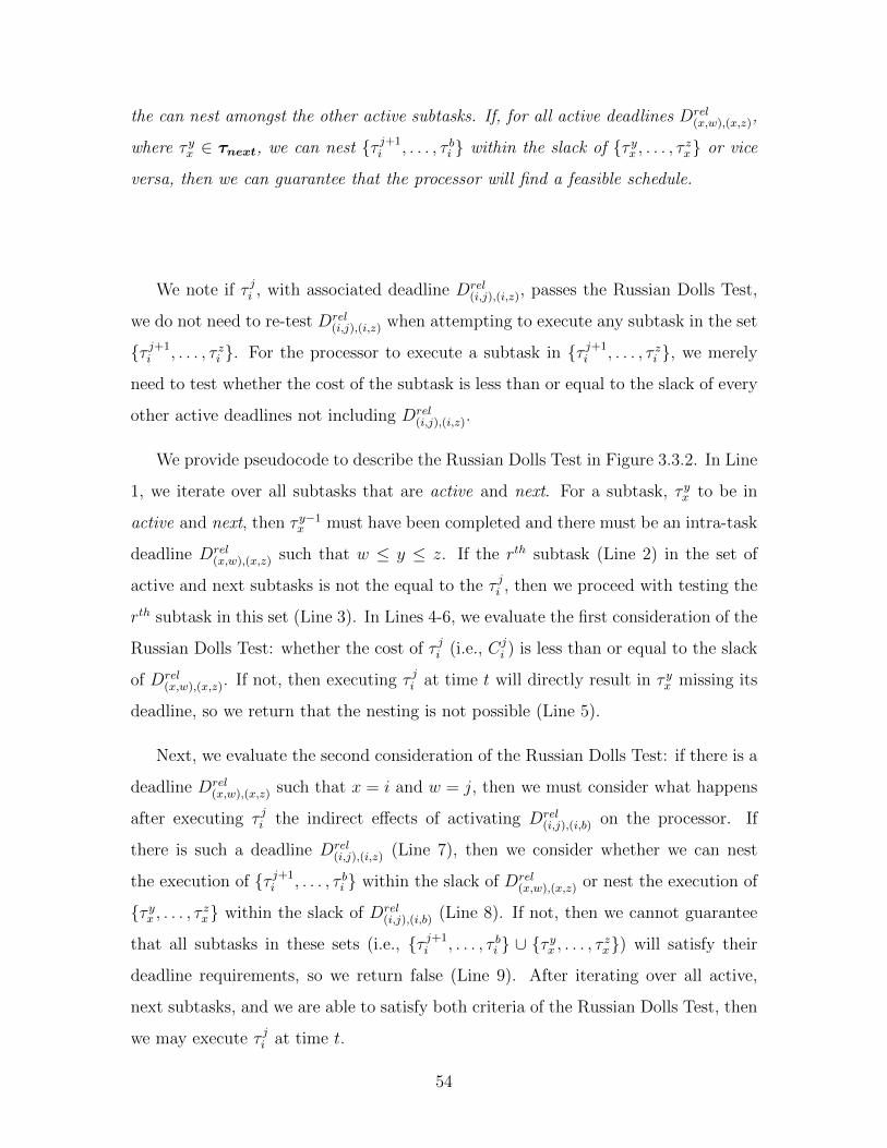
the can nest amongst the other active subtasks. If, for all active deadlines Drel(x,w),(x,z),
where τ yx ∈ τnext, we can nest {τ j+1i , . . . , τ bi } within the slack of {τ yx , . . . , τ zx} or vice
versa, then we can guarantee that the processor will find a feasible schedule.
We note if τ ji , with associated deadline Drel(i,j),(i,z), passes the Russian Dolls Test,
we do not need to re-test Drel(i,j),(i,z) when attempting to execute any subtask in the set
{τ j+1i , . . . , τ zi }. For the processor to execute a subtask in {τ j+1
i , . . . , τ zi }, we merely
need to test whether the cost of the subtask is less than or equal to the slack of every
other active deadlines not including Drel(i,j),(i,z).
We provide pseudocode to describe the Russian Dolls Test in Figure 3.3.2. In Line
1, we iterate over all subtasks that are active and next. For a subtask, τ yx to be in
active and next, then τ y−1x must have been completed and there must be an intra-task
deadline Drel(x,w),(x,z) such that w ≤ y ≤ z. If the rth subtask (Line 2) in the set of
active and next subtasks is not the equal to the τ ji , then we proceed with testing the
rth subtask in this set (Line 3). In Lines 4-6, we evaluate the first consideration of the
Russian Dolls Test: whether the cost of τ ji (i.e., Cji ) is less than or equal to the slack
of Drel(x,w),(x,z). If not, then executing τ ji at time t will directly result in τ yx missing its
deadline, so we return that the nesting is not possible (Line 5).
Next, we evaluate the second consideration of the Russian Dolls Test: if there is a
deadline Drel(x,w),(x,z) such that x = i and w = j, then we must consider what happens
after executing τ ji the indirect effects of activating Drel(i,j),(i,b) on the processor. If
there is such a deadline Drel(i,j),(i,z) (Line 7), then we consider whether we can nest
the execution of {τ j+1i , . . . , τ bi } within the slack of Drel
(x,w),(x,z) or nest the execution of
{τ yx , . . . , τ zx} within the slack of Drel(i,j),(i,b) (Line 8). If not, then we cannot guarantee
that all subtasks in these sets (i.e., {τ j+1i , . . . , τ bi } ∪ {τ yx , . . . , τ zx}) will satisfy their
deadline requirements, so we return false (Line 9). After iterating over all active,
next subtasks, and we are able to satisfy both criteria of the Russian Dolls Test, then
we may execute τ ji at time t.
54
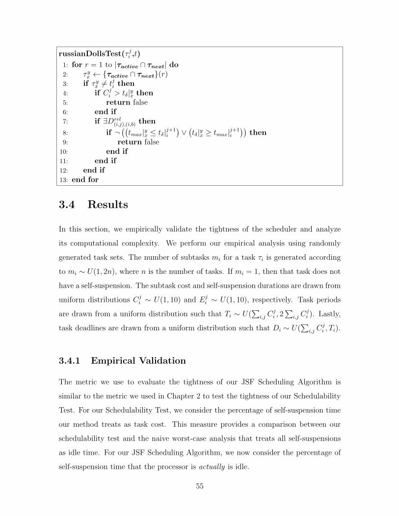
russianDollsTest(τ ji ,t)
1: for r = 1 to |τactive ∩ τnext| do2: τ yx ← {τactive ∩ τnext}(r)3: if τ yx 6= tji then4: if Cj
i > tδ|yx then5: return false6: end if7: if ∃Drel
(i,j),(i,b) then
8: if ¬((tmax|yx ≤ tδ|j+1
i
)∨(tδ|yx ≥ tmax|j+1
i
))then
9: return false10: end if11: end if12: end if13: end for
3.4 Results
In this section, we empirically validate the tightness of the scheduler and analyze
its computational complexity. We perform our empirical analysis using randomly
generated task sets. The number of subtasks mi for a task τi is generated according
to mi ∼ U(1, 2n), where n is the number of tasks. If mi = 1, then that task does not
have a self-suspension. The subtask cost and self-suspension durations are drawn from
uniform distributions Cji ∼ U(1, 10) and Ej
i ∼ U(1, 10), respectively. Task periods
are drawn from a uniform distribution such that Ti ∼ U(∑
i,j Cji , 2∑
i,j Cji ). Lastly,
task deadlines are drawn from a uniform distribution such that Di ∼ U(∑
i,j Cji , Ti).
3.4.1 Empirical Validation
The metric we use to evaluate the tightness of our JSF Scheduling Algorithm is
similar to the metric we used in Chapter 2 to test the tightness of our Schedulability
Test. For our Schedulability Test, we consider the percentage of self-suspension time
our method treats as task cost. This measure provides a comparison between our
schedulability test and the naive worst-case analysis that treats all self-suspensions
as idle time. For our JSF Scheduling Algorithm, we now consider the percentage of
self-suspension time that the processor is actually is idle.
55
Figure 3-2: Percentage of self-suspension time that the processor is is idle.
Figure 3-2 presents the empirical results of evaluating the tightness of our JSF
scheduling algorithm for randomly generated task sets with 2 to 20 tasks, and Figure
3-3 includes the tightness of the schedulability test for comparison. Each data point
and error bars represent the mean and standard deviation valuated for ten randomly
generated task sets. D denotes the ratio of subtasks that are released during the
hyperperiod and constrained by intra-task deadline constraints to the total number
of subtasks released during the hyper period. We see the amount of idle time due to
self-suspensions is inversely proportional to problem size. For large problems, our JSF
scheduling algorithm produces a near-zero amount of idle time due to self-suspensions
relative to the total duration of all self-suspensions during the hyperperiod.
56
Figure 3-3: Percentage of self-suspension time that the processor is is idle comparedto the percentage of self-suspension time the schedulability test assumed as idle time.
57
3.4.2 Computational Complexity
We upperbound the computational complexity of our JSF Scheduling Algorithm at
each time step. At each time step, the processor must consider n tasks in the worst
case. For each of the n tasks, the scheduler would call russianDollsTest(τ ji ). In the
worst case, the number of active deadlines is upperbounded by n; thus, the complexity
of the Russian Dolls Test is O(n). In turn, the JSF Scheduling algorithm performs
at most O(n2) operations for each time step.
3.5 Conclusion
We have presented a uniprocessor scheduling algorithm for hard, non-preemptive,
self-suspending task sets with intra-task deadline constraints and . Our polynomial-
time scheduling algorithm leverages problem structure by scheduling according to
the jth subtask first (JSF) scheduling policy that we developed in Chapter 2. Our
algorithm also utilizes an polynomial-time, online consistency test to ensure temporal
consistency due to intra-task deadlines, called the Russian Dolls Test. Although
the JSF policy and Russian Dolls Test are not optimal, we show through empirical
evaluation that our scheduling algorithm produces schedules that are within a few
percent of the best possible makespan.
58
Chapter 4
Multiprocessor Scheduling Policy
4.1 Introduction
In Chapter 3, we present a near-optimal method for uniprocessor scheduling of hard,
non-preemptive, self-suspending task sets. These task sets were defined by at least
one subtask per task, intra-task deadlines, and phase offsets. In this chapter, we
extend our method for scheduling uniprocessor systems to handle multiprocessor sys-
tems. We use this extension in Chapter 5 to develop a task allocation and scheduling
algorithm for robotic manufacturing of aerospace structures. To schedule these tasks
sets, we need to incorporate spatial constraints (i.e., shared memory resources) to
ensure that agents do not interfere with each other in space (e.g., collisions). In Sec-
tion 4.2, we extend the self-suspending task model we present in Chapters 2 and 3
for the multiprocessor case. We next extend some of the terminology we introduced
in Chapters 2-3 to the multiprocessor case in Section 4.3 In Section 4.4, we present
our scheduling policy. In Section 4.5, we analyze the computational complexity of
our algorithm, and we conclude in Section 4.6.
4.2 Our Augmented Task Model
In Chapter 2, we present the self-suspending task model we use to better reflect the
constraints of interest (Equation 2.1). For the multiprocessor case, we incorporate
59
both an assignment of processors to subtasks (i.e., task allocation) and shared memory
resources as shown in Equation 4.1. In this model, Ri = {R1i , R
2i , . . . , R
mi } is the set of
shared memory resource constraints such thatRji is the set of shared memory resources
require to execute τ ji . Ai = {A1i , A
2i , . . . , A
mi } is the processor allocation for τi such
that Aji is the processor assigned to execute τ ji . Furthermore we restrict the periodicity
and absolute deadline of all tasks to be equal to a user-specified hyperperiod. This
constraint corresponds to a pulse-line in the manufacturing environment where all
tasks in the task set must be accomplished once every pulse of the line.
τi : (φi, (C1i , E
1i , C
2i , E
2i , . . . , E
mi−1
i , Cmii ), Ri, Ai, Ti = H,Di = H,Drel
i ,Dabsi ) (4.1)
In addition to intra-task deadlinesDreli for τi, we extend our task model to include
subtasks deadlines, where Dabsi is the set of subtask deadlines for subtasks in τi. As
shown in Equation 4.2, if a subtask τ ji is constrained by a subtask deadline constraint,
then f ji must not exceed dabsi,j .
Dabsi,j :
(f ji ≤ dabsi,j
)(4.2)
4.3 Terminology
In this section we extend the terminology from Chapter 3 to help describe our multi-
processor scheduling algorithm. In Section 4.4, we use the terms to aid in explaining
how we can ensure temporal consistency due to absolute subtask deadlines. In Chap-
ter 3, we defined a subtask group, active intra-task deadline and active subtasks. We
now augment the definitions of a subtask group and an active subtask to include
absolute subtask deadline; we also define a new term: active subtask deadline.
Definition 14. A subtask group, Gji , is an ordered set of subtasks that share a com-
mon deadline constraint. If we have a deadline constraint D(i,a),(i,b), then the subtask
group for that deadline constraint would be the Gji = {τ yi |j ≤ y ≤ b}. If we have
a subtask deadline constraint Dabsi,j , then a subtask group for that deadline constraint
60
would be the Gai = {τ yi |a ≤ y ≤ j}. Furthermore, Gj
i (k) returns the kth element of
Gji , where the set is ordered by subtask index (e.g., y associated with τ yi ).
Definition 15. An active subtask deadline is a subtask deadline constraint, Dabsi,j ,
where the processor has not finished τ ji . Formally Dabsactive = {Dabs
i,j |Dabsi,j ∈ Dabs, 0 ≤
t < f ji }, where Dabs is the set of all intra-task deadlines.
Definition 16. The set of active subtasks, τactive, are the set of all unfinished
subtasks associated with active intra-task deadlines or subtask deadlines. Formally
τactive = {τ ji |τji ∈ τ ,
(∃Drel
(i,a),(i,b) ∈Drel, a ≤ j ≤ b, sai ≤ sji ≤ t < f bi
)∨(∃Dabs
i,a ∈Dabs, 1 ≤ j ≤ a, 0 ≤ t < fai)}.
4.4 Multiprocessor Scheduling Algorithm
Our multiprocessor algorithm (Figure 4.4.1) receives as input a self-suspending task
set, τ , according to Equation 4.1, and terminates after scheduling all subtasks. Be-
cause these tasks have a uniform periodicity, only one instance of each task is sched-
uled. The algorithm steps through time to schedule released tasks in τ . The order
with which processors attempt to schedule subtasks is based on an processor-priority
heuristic, and the order with which subtasks assigned to a given processor are con-
sidered by that processor is based on a set of subtask priorities. The scheduler only
schedules a subtask iff an online consistency test (i.e., our Multiprocessor Russian
Dolls Test) guarantees that doing so does not result in violating another temporal or
We now step through the mechanics of our scheduling algorithm. In Line 1, we tighten
the intra-task deadlines and subtask deadlines to produce better problem structure.
We note that, for the uniprocessor case (Chapter 3.3), we only considered intra-task
deadlines. The self-suspending task model for the multiprocessor case (Equation 4.1)
includes intra-task deadlines and subtask deadlines. These deadlines may “overlap”,
61
multiprocessorSchedulingAlgorithm(τ )
1: Drel,Dabs ← simplifyDeadlines(Drel,Dabs)2: if ∃Dabs
i,j ∈Dabs then
3: if ¬multiprocessorRussianDollsTest(τ ji ,τ ,0,1) then4: return null5: end if6: end if7: t← 08: while TRUE do9: A ← prioritizeAgents(A);10: for α = 1 to |A| do11: if processor a is idle then12: availableSubtasks ← getAvailableSubtasks(t,a);13: availableSubtasks ← prioritizeTasks(availableSubtasks);14: for (k = 1 to |availableTasks|)) do15: τ ji ← availableTasks[k];16: if multiprocessorRussianDollsTest(τ ji ,τ ,t,0) then17: scheduleProcessor(τ ji ,t,α)18: scheduleResource(τ ji ,ts,R
ji )
19: break20: end if21: end for22: end if23: end for24: if all tasks in τ have been finished then25: return schedule26: else27: t← t+ 128: end if29: end while
Figure 4-1: Pseudocode describing the multiprocessor scheduling algorithm.
62
meaning that there are at least two deadline constraints who’s interaction can cate-
gorized by one of three cases:
1. Drel(i,a),(i,b) and Drel
(i,y),(i,z) such that a ≤ y ≤ b, which we considered in Chapter 3
2. Dabsi,a and Dabs
i,b such that a ≤ b.
3. Drel(i,a),(i,b) and Dabs
i,j such that a ≤ b.
To tighten the deadlines for all three cases, we can apply the methodology described
in Chapter 3 Section 3.3 with augmented formulae to handle subtask deadlines. In-
tuitively, we remove two overlapping deadline constraints and replace each pair with
a new deadline constraint such that any schedule that satisfies the new deadline also
satisfies the original deadlines.
For case one where we have two overlapping intra-task deadlines Drel(i,a),(i,b) and
Drel(i,y),(i,z)), we can apply Equations 4.3 and 4.5. For case two where we have two
overlapping absolute deadlines Dabsi,a and Dabs
i,b , we can apply Equations 4.4 and 4.6.
Finally, for case three where we have an overlapping intra-task deadline constraint
and a subtask deadline constraint, we can apply Equations 4.3 and 4.3 for the dead-
lines’ slack and Equation 4.7 to compute the tightness of the new absolute deadline
constraint. After replacing all overlapping deadlines such that there are no remaining
overlapping in the task set, we proceed to scheduling the task set.
TERCIO-SEQUENCER(A, STP,R, cutoff)7: end while8: STP ← add ordering constraints to enforce seq9: STP ← DISPATCHABLE(STP )10: return STP
Figure 5-2: Psuedo-code for the Tercio Algorithm.
problems.
5.5 Tercio
In this section, we present Tercio, a centralized task assignment and scheduling al-
gorithm that scales to multi-agent, factory-size problems and supports on-the-fly re-
planning with temporal and spatial-proximity constraints. Pseudo-code for the Tercio
algorithm is presented in Figure 5-2.
The inputs to Tercio are as described in Section 5.3. Tercio also takes as input a
user-specified makespan cutoff (Line 2) to terminate the optimization process. This
can often be derived from the temporal constraints of the manufacturing process. For
example, a user may specify that the provided task set must be completed within an
eight-hour shift. Tercio then iterates (Lines 3-7) to compute an agent allocation and
schedule that meets this makespan. Because Tercio uses a satisficing and incomplete
sequencer, it is not guaranteed to find an optimal solution, or even a satisficing solu-
tion if one exists. In practice, we show (Section 5.7) Tercio produces makespans within
about 10% of the optimal minimum makespan, for real-world structured problems.
81
5.5.1 Tercio: Agent Allocation
Tercio performs agent-task allocation by solving a simplified version of the MILP
from Section 5.3. The objective function for the agent allocation MILP is formulated
as follows:
min(z), z = f1(A,P, γ) + f2(A) + v (5.10)
where, recall g minimizes the difference between the previous agent assignment and
the returned agent assignment to help avoid oscillations between equivalent quality
solutions during replanning, and h minimizes the number of spatial interfaces between
tasks performed by different robots.
We introduce a proxy variable v into the objective function to perform work-
balancing and guide the optimization towards agent allocations that yield a low
makespan. The variable v encodes the maximum total task time that all agents
would complete their tasks, if those tasks had no deadline or delay dependencies and
is defined as:
v ≥∑j
cj × Aa,j∀a ∈ A (5.11)
where cj is a constant representing the expected time of each task. We find in practice
the addition of this objective term and constraint guides the solution to more efficient
agent allocations. The agent allocation MILP must also include Equations 5.2 and 5.3
ensuring each task is assigned to exactly one agent and that the agent-task allocation
does not violate the STP constraints.
5.5.2 Tercio: Pseudocode
A third-party optimizer [1] solves the simplified agent-allocation MILP (Line 4)
and returns the agent allocation matrix A. Interval temporal (STP) constraints are
updated based on this agent allocation matrix by tightening task time intervals (Line
5). For example, if a task is originally designated to take between five and fifteen
minutes but the assigned robot can complete it no faster than ten minutes, we tighten
82
the interval from [5, 15] to [10, 15].
The agent allocation matrix, the capability-updated STP, and the spatial map of
tasks are then provided as input to the Tercio multi-agent task sequencer (Line 6).
The task sequencer (described further in Section 5.6) returns a tight upperbound on
the optimal makespan for the given agent allocation as well as a sequence of tasks for
each agent.
While this makespan is longer than cutoff , the algorithm iterates (Lines 3-7), each
time adding a constraint (Line 3) to exclude the agent allocations tried previously:
∑a,i|La,i=0
Aa,i +∑
a,i|La,i=1
(1− Aa,i) > 0 (5.12)
where La,i is the solution from the last loop iteration.
Tercio terminates when the returned makespan falls beneath cutoff , or else when
no solution can be found after iterating through all feasible agent allocations. If the
cutoff makespan is satisfied, agent sequencing constraints (interval form of [0,∞))
are added to the STP constraints (Line 8). Finally the resulting Simple Temporal
Problem is compiled to a dispatchable form (Line 9) [38, 52], which guarantees
that for any consistent choice of a timepoint within a flexible window, there exists
an optimal solution that can be found in the future through one-step propagation of
interval bounds. The dispatchable form maintains flexibility to increase robustness to
disturbances, and has been shown to decrease the amount of time spent recomputing
solutions in response to disturbances by up to 75% for randomly generated structured
problems [52].
5.6 Tercio: Multi-agent Task Sequencer
The key to increasing the computational speed of Tercio is our hybrid approach
to task sequencing. Tercio takes as input a set of agent-task assignments and a
well-formed self-suspending task model (defined below), and returns a valid task
sequence if one can be found by the algorithm. The task sequencer is merely satisficing
83
and is not complete; however, we empirically validate that it returns near-optimal
makespans when integrated with the Tercio Agent Allocation algorithm (See Section
5.7). In this section, we provide an overview of the multi-agent task sequencer by first
introducing our task model, which is inspired by real-time systems scheduling. Second
we describe how our fast task sequencer works to satisfy temporospatial constraints.
A full treatment can be found in Chapter 4.
5.6.1 Well-Formed Task Model
The Tercio Task Sequencer relies on a well-formed task model that captures hierar-
chical and precedence structure in the task network. The basis for our framework is
the self-suspending task model [33], described in Equation 5.13.
τi : ((C1i , E
1i , C
2i , E
2i , . . . , E
mi−1
i , Cmii ), Ai, Ti, Di). (5.13)
In this model, there is an instance, I, with a set of tasks, τ , that must be processed
by the computer. For each task, there are mi subtasks with mi − 1 self-suspension
intervals for each task τi ∈ τ . We use τ ki to denote the kth subtask of τi, Cki is the
expected duration (cost) of τ ki . Eki is the expected duration of the kth self-suspension
interval of τi. Ti and Di are the period and deadline of τi, respectively. Furthermore,
subtask τ ji is assigned to processor Aji .
The standard self-suspending task model provides a solid basis for describing many
real-world processor scheduling problems of interest. In this work we present an
augmented model to better capture problem structure inherent in the manufacturing
environment:
τi : (φi, (C1i , E
1i , . . . , E
mi−1
i , Cmii ), Ai, Ti = H,Di = H,Drel
i ,Dabsi ,Ri) (5.14)
where we set the implicit deadlines of the tasks equal to the period of the task set.
This modification models well many assembly line manufacturing processes where the
set of tasks at one location is repeated once every “pulse” of the production line. In
84
this scenario, the user allots a certain amount of time, T , for the set of tasks to be
accomplished, and the set of tasks is repeated with a period of T . For convenience,
we will not explicitly state (Ti = T,Di = T ) from Equation 5.14 in the remainder of
the paper; however, these constraints are implied. For convenience, we also assume
all tasks are non-preemptable, meaning the interruption of a subtask significantly
degrades its quality.
The second adaptation we make is to allow phase offsets for each task, where a
phase offset is a delay between the epoch time and the release of the given task. This
allows a user expressiveness to require that an agent wait a specified time interval
before starting the first subtask of a task.
The third change we make is to enable the user to specify intra-task deadlines,
Drel(i,j),(i,b) between the start and end of two subtasks for a given task and subtask
deadlines, Dabsi,j for an individual subtask. We define an intra-task deadline in Equa-
tion 5.15 and a subtask deadline in Equation 5.16. The set of intra-task deadlines for
τi is Dreli .
Drel(i,j),(i,b) :
(f(τ bi )− s(τ ji ) ≤ d(i,j),(i,b)
)3 1 ≤ j ≤ b ≤ mi (5.15)
Dabs(i,b) :
(f(τ bi ) ≤ dabs(i,b)
)3 1 ≤ b ≤ mi (5.16)
where the operator f bi is the finish time of subtask τ bi , sji is the start time of sub-
task τ ji . For Equation 5.15, drel(i,j),(i,b) is the upperbound temporal constraint between
τ ji and τ bi . For Equation 5.16 dabsi,b is the absolute deadline for τ bi . This deadline
constraints provide additional expressiveness to encode binary temporal constraints
relating tasks in the manufacturing process. For instance, these constraints may be
used to specify that a sequence of subtasks related to sealant application must be
completed within a half hour after opening the sealant container. These types of
constraints are commonly included in AI and operations research scheduling models
[5, 14, 38, 52].
We also extend the model to include shared memory resources. Each subtask
τ ji requires a set of ki shared memory resources Rji = {R1
i,j, . . . , Rkii,k} be utilized to
85
perform that subtask (e.g. for memory shared among multiple processors). In the
manufacturing analogy, a shared memory resource corresponds to a region of space
in the factory that must physically be unoccupied for an agent to execute a subtask
there. These shared memory resources are used to encode hard spatial constraints
that prohibit agents from working in close physical proximity.
Next we describe how the Tercio Task Sequencer leverages the structure of the well-
formed task model to compute a schedule that satisfies upperbound and lowerbound
temporal constraints, as well as spatial-proximity restrictions. To our knowledge,
this is the first real-time scheduling method for multi-processor systems that (1) tests
the schedulability of self-suspending, non-preemptive tasks where multiple tasks in τ
have more than one self-suspension [33, 32, 43], and (2) that extends self-suspending
models to include shared memory resources.
5.6.2 Multi-agent Task Sequencer Overview
The Tercio multi-agent task sequencer pseudo-code takes as input a task set τ of
a well-formed task model (also called the STP constraints) and the user-specified
makespan cutoff . The algorithm returns a valid task sequence for each agent, if one
can be found, and an upperbound on the time to complete all tasks. This upperbound
on completion time is compared to cutoff to test schedulability of a well-formed task
model.
Restriction on the Behavior of the Scheduler
We introduce three task-based heuristic restrictions an agent based heuristic restric-
tion and on the scheduling simulation that address the types of schedule bottlenecks
that hinder efficient execution in the well-formed task model augmented with shared
memory resources.
First, we introduce a heuristic πp(τji ) (Equation 4.8) to ease bottlenecks due to
inter-agent precedence constraints. Second, we introduce a heuristic πR(τ ji ) (Equation
4.9) that prioritizes subtasks according to the number of other subtasks in the model
86
that will require the same resource. Lastly, we introduce a heuristic πl(τji ) (Equation
4.10) to reduce travel distance. While travel time is small relatively to the task
durations of interest, we do not want robots to move erratically about the space from
the point of view of their human teammates.
These three heuristics can be combined in various formulations. We have chosen
a tiered system, in which tasks are ordered according to one heuristic. Then, for all
tasks that have the same value based on the first heuristic, those tasks are ordered
according to a second heuristic. This process is repeated for the last heuristic. The
order in which the heuristics are applied can be tuned a priori with the knowledge
of what kind of bottlenecks govern the system. For our real-world problems in large-
scale assembly manufacturing, we find the the key bottleneck is the need to satisfy
precedence constraints between subtasks assigned to different agents. For the results
discussed in this paper, we order the heuristics as follows: 1) πp(τji ), 2) πR(τ ji ), 3)
πl(τji ).
We also use an agent-based heuristic to improve the efficiency of the schedule.
The order with which agents are scheduled is chosen based on how many released,
unexecuted subtasks are assigned to the agents. When each agent is scheduled, the
domain of subtasks that can be correctly scheduled either is unchanged or decreases. If
an agent with relatively few subtask options schedules last, that agent may be forced
to idle because of constraints imposed by the other agents schedules. Therefore,
we prioritize the order with which agents are scheduled such that agents with more
released, unexecuted subtasks schedule after those with fewer released, unexecuted
subtasks.
Finally, our scheduling policy requires that an agent not idle if there is an avail-
able subtask, unless executing that subtask will violate a subtask-to-subtask deadline
constraint. This condition is checked via an online temporospatial consistency test.
Multi-Agent Online Consistency Check.
During the scheduling simulation, we perform an online consistency check, which
we call the Multiprocessor Russian Dolls Test (Chapter 4), that ensures that the
87
scheduling of a next subtask, τ ji , will not result a missed deadline for a different
subtask, τ yx , or violate a spatial-proximity constraint. Note, by the definition of a
well-formed task model, τi and τj must be different tasks for their subtasks to be
scheduled concurrently.
Our well-formed self-suspending task model includes absolute deadlines, Dabs(i,b)
relating a subtask τ bi to the plan epoch time, and inter-subtask deadline, D(i,j),(i,b),
from τ ji to τ bi . We now introduce a definition for the an active deadline, which we use
to describe our online consistency test.
Definition 23. Active Deadline - Consider an intra-task deadline Drel(i,j),(i,b), or an
absolute deadline Dabsi,j . An intra-task deadline is considered active between 0 ≤ t ≤
min(fi,j, Drel(i,j),(i,b)), and an absolute deadline is considered active between 0 ≤ t ≤
min f ji , Dabsi,j .
We readily formulate our online consistency test as a constraint satisfaction prob-
lem. First, we will consider the case where we have multiple, active, inter-task dead-
lines. We evaluate Equations 5.17-5.22 for the union of all active deadlines and the
deadline we are considering activating.
δa(i,j),(i,k) ≥ γa(x,y),(x,z),∀Dβa(x,y,z,a)i D
βa(i,j,k,a)i ,∀a ∈ A (5.17)
δai,j:k = γa(i,j),(i,k) −(Cβa(i,j,k,a)i +
∑βa(i,j,k,a)−1ψ=ξa(i,j,k,a)
(Cψi + Eψ
i ))
(5.18)
γa(x,y),(x,z) = Dβ(i,j,k,a)i − t (5.19)
δr(i,j),(i,k) ≥ γr(x,y),(x,z),∀Dβr(x,y,z,r)i D
βr(i,j,k,r)i ,∀r ∈ R (5.20)
δri,j:k = γr(i,j),(i,k) −(Cβr(i,j,k,r)i +
∑βr(i,j,k,a)−1ψ=ξr(i,j,k,r)
(Cψi + Eψ
i ))
(5.21)
γr(x,y),(x,z) = Dβ(i,j,k,r)i − t (5.22)
Equation 5.17 determines whether or not we can “nest” a set of tasks within the
“slack time” of the deadline associated with another set of tasks. Specifically, we
must ensure that γa(i,j),(i,k), defined as the amount of time an agent a is occupied with
subtasks {τ ji , . . . , τ ki } associated with Drel(i,j),(i,k) (or Dabs
i,k where j = 1), is less than
88
the slack time, δax,y:z, for the agent a’s other commitments to {τ ji , . . . , τ ki } associated
with active deadline Drel(x,y),(x,z) or D(x, y)abs. Slack is calculated in Equations 5.18-
5.19, where ξa(i, j, k, a) and βa(i, j, k, a) refer respectively the next and last subtask
to which agent a is assigned to in {τ ji , . . . , τ ki }.
We utilize the same methodology for spatial constraints in Equations 5.17- 5.19.
Specifically, we test whether γr(i,j),(i,k), defined as the amount of time an resource r is
occupied with subtasks {τ ji , . . . , τ ki } associated with Drel(i,j),(i,k) or Dabs
i,k , is less than the
slack time, δrx,y:z, for the resource r’s other commitments to {τ ji , . . . , τ ki } associated
with active deadline Drel(x,y),(x,z) or D(x, y)abs.
Our multi-agent sequencer uses a polynomial-time version of this online consis-
tency test to evaluate the feasibility of scheduling subtasks. A full description of the
online consistency test is provided in Chapter 4 Section 4.4.2. The complexity of this
consistency check is O(n(a + r)) where n is the number of tasks, a is the number of
agents, and r is the number of resources.
5.7 Evaluation and Discussion
In this section, we empirically validate that Tercio is fast and produces near-optimal
solutions for the multi-agent task assignment and scheduling problem with temporal
and spatial-proximity constraints.
5.7.1 Generating Random Problems
We evaluate the performance of Tercio on randomly generated, structured problems
that simulate multi-agent construction of a large structural workpiece, such as an
airplane fuselage or wing.
Task times are generated from a uniform distribution in the interval [1, 10]. Ap-
proximately 25% of the subtasks are related via a nonzero wait duration (lowebound
constraint) drawn from the interval [1, 10], and approximately 25% of the subtasks
are related via an upperbound temporal deadline generated randomly to another sub-
task. The upperbound of each deadline constraint, Drel(i,j),(x,y), is drawn from a normal
89
distribution with mean set to the lowerbound temporal duration between the start
and end of the set of subtasks in Drel(i,j),(x,y). Physical locations of a subtask are drawn
from a uniform distribution in [1, n] where n is the total number of subtasks in the
problem instance, τ . Lastly, we vary the number of subtasks, mi, within each task,
τi, from a uniform distribution in the interval [0.25× numTasks, 1.25× numTasks],
where numTasks is the number of τi ∈ I.
5.7.2 Computation Speeds
In Figure 5-3 we evaluate scalability and computational speed of Tercio. We show
the median and quartiles of computation time for 25 randomly generated problems,
spanning 4 and 10 agents, and 5 to 500 tasks (referred to as subtasks in the well-
formed model). For comparison, we show computation time for solving the full MILP
formulation of the problem, described in Section 5.3. Tercio is able to generate flexible
schedules for 10 agents and 500 tasks in seconds. This is a significant improvement
over prior work [9, 10, 49, 30], which report solving up to 5 agents (or agent groups)
and 50 tasks in seconds or minutes.
5.7.3 Optimality Levels
Our fast computation relies on the known structure of our well-formed task model,
but it is desirable to be able to take as input general sets of temporal (STP) con-
straints. General STPs can be reformulated into well-formed task models by adding
and tightening well-formed temporal constraints to make the constraints that violate
the well-formed model redundant. We present results with both random problems
that are well-formed and problems that are general but have been reformulated into
a well-formed task model.
In Figures 5-4-5-5 we show that Tercio is often able to achieve makespans within
10% of the optimal makespan for well-formed models and 15% of the optimal makespan
for general STPs; Tercio is also able to produce less than four additional interfaces
when compared to the optimal task allocation for well-formed models and less than
90
Figure 5-3: Empirical evaluation: computation speed as function of number of workpackages and number of agents. Results generated on an Intel Core i7-2820QM CPU2.30GHz.
91
Figure 5-4: Empirical evaluation: Tercio suboptimality in makespan for problemswith 4 agents.
eight additional interfaces for general models. We are unable to measure the subop-
timality gap for larger problem instances due to the computational intractability of
the full MILP. The purpose of Tercio is to solve the problem of scheduling with tens
of agents and hundreds of tasks; as we can see in Figure 5-4, Tercio tightly tracks the
optimal solution.
5.7.4 Robot Demonstration
We demonstrate the use of Tercio to plan the work of two KUKA Youbots. Video
can be found at http://tiny.cc/t6wjxw. The two robots are working to assemble a
mock airplane fuselage. The robots perform their subtasks at specific locations on the
factory floor. To prevent collisions, each robot reserves both the physical location for
its subtask, as well as the immediately adjacent subtask locations. Initially, the robots
plan to split twelve identical tasks in half down the middle of the fuselage. After the
robots finish their first subtasks, a person requests time to inspect the work completed
on the left half of the fuselage. In the problem formulation, this corresponds to adding
a resource reservation for the left half of the fuselage for a specified period of time.
Tercio replans in response to the addition of this new constraint, and reallocates the
Figure 5-5: Empirical evaluation: Tercio suboptimality in number of interfaces forproblems with 4 agents.
Figure 5-6: Hardware demonstration of Tercio. Two KUKA Youbots build a mockairplane fuselage. A human worker requests time on the left half of the fuselage toperform a quality assurance inspection, and the robots replan.
93
work among the robots in a near-optimal manner to make productive use of both
robots and to keep the number of interfaces low.
5.8 Conclusion
We present Tercio, a task assignment and scheduling algorithm that is made efficient
through a fast, satisficing, incomplete multi-agent task sequencer inspired by real-
time processor scheduling techniques. We use the fast task sequencer in conjunction
with a MILP solver to compute an integrated multi-agent task sequence that satisfies
precedence, temporal and spatial-proximity constraints. We demonstrate that Tercio
generates near-optimal schedules for up to 10 agents and 500 tasks in less than 20
seconds on average.
94
Chapter 6
Towards Successful Coordination
of Human and Robotic Work using
Automated Scheduling Tools: An
Initial Pilot Study
6.1 Introduction
In this chapter, we will seek to understand how much control human workers should
have over the assignment of roles and schedules, when working in a team with robot
partners. Successful integration of robot systems into human teams requires more
than tasking algorithms that are capable of adapting online to the dynamic envi-
ronment. The mechanisms for coordination must be valued and appreciated by the
human workers.
Human workers often find identity and security in their roles or jobs in the factory
and are used to some autonomy in decision-making. A human worker that is instead
tasked by an automated scheduling algorithm may begin to feel that he or she is
diminished. Even if the algorithm increases process efficiency at first, there is concern
that taking control away from the human workers may alienate them and ultimately
95
damage the productivity of the human-robot team. The study of human factors
can inform the design of effective algorithms for collaborative tasking of humans and
robots.
In this work, we present results from a pilot study (n = 8) where participants
collaborate with a robot on a construction task. In one condition, both the human
and robot are tasked by Tercio, the automatic scheduling algorithm. In the second
condition, the human worker is provided with a limited set of task allocations from
which he/she can choose. We hypothesize that giving the human more control over
the decision-making process will increase worker satisfaction, but that doing so will
decrease system efficiency in terms of time to complete the task.
We begin in Section 6.2 with a brief review of related work in human factors stud-
ies of human-machine systems and task allocation. In Section 6.3 and Section 6.4 we
describe our experimental method and we report the results from the human subject
experiment. We then discuss the implications, limitations, and lessons learned from
the results of our pilot study in Section 6.5. In Section 6.6, we discuss recommenda-
tions for a full human subjects experiment. Lastly, we summarize our findings and
discuss future work in Section 6.7. For a full description of Tercio, see Chapter 5.
6.2 Background
Developing man-machines systems that are able to leverage the strengths of both
humans and their artificial counterparts has been focus of much attention from both
human factors engineers as well as researchers in artificial intelligence. Parasuraman
has pioneered work examining adaptive automation to regulate operator workload
[40]. When the operator is over-tasked, the automation can reduce the burden on the
operator by assuming certain tasks. If the human-automation system experiences a
period of low workload, the automation can shift more responsibility to the human
operator to mitigate possible complacency or a reduction in manual skills [39].
The human-robot interface has long been identified as a major bottleneck in utiliz-
ing these robotic systems to their full potential [7]. As a result, we have seen significant
96
research efforts aimed at easing the use of these systems in the field, including careful
design and validation of supervisory and control interfaces [4, 12, 23, 28]. Other,
related research efforts have focused on utilizing a human-in-the-loop to improve the
quality of task plans and schedules [11, 12, 16]. This is particularly important when
the search space is large or if it is not possible to represent all aspects of the environ-
ment in the problem formulation.
These prior efforts have focused primarily on utilizing a human-in-the-loop to
improve plans and schedules for work performed by other agents. In this work, we
are motivated by applications in the manufacturing domain where human workers will
be performing physical tasks in coordination with robotic partners. In some cases,
the human workers may also be responsible to tracking the progress and tasking the
team. We seek to understand how much control human workers should have over
the assignment of roles and schedules, when working in teams with robots. While we
necessarily want to maximize the efficiency of human-robot teams, we also desire for
the human workers to value, accept, and cooperate with the new technology. With
this in mind, the following sections of this paper will describe the pilot study we
conducted to lend insight into trade-offs among flexibility in decision-making, overall
task efficiency, and worker satisfaction.
6.3 Methods
The purpose of this pilot study is to gain insight into how to integrate multi-agent
task allocation and scheduling algorithms to improve the efficiency of coordinated
human and robotic work. We hypothesize that keeping the human worker in the
decision making process by letting him/her decide the task assignments will decrease
performance of the system (i.e., increase time to complete the task objective) but will
increase the human appreciation of the overall system. We conducted a pilot study
to assess the tradeoffs in task efficiency and user satisfaction, depending on whether
or not the worker is allowed control over task allocation.
For our pilot study, we consider two experimental conditions:
97
• Condition 1: A task allocation and scheduling algorithm (i.e., Tercio [22]) spec-
ifies the plan.
• Condition 2: The human worker is given a limited set task allocations from
which he/she can choose.
6.3.1 Experimental Setup
The task objective given to the human-robot team is to complete two Lego kits, each
consisting of seven steps. The parts required to build each of the seven steps for both
Lego kits are placed into bins away from the build area. There are two classes of roles
for the agents: builder or a part fetcher. If an agent is a builder, then the agent is
responsible for building either one or both of the Lego kits. If an agent is a fetcher,
that agent retrieves part bins and transports them to a specified builder. We enforce
that the fetcher can only fetch one part bin at a time.
If a robot is assigned to fetch parts, we must have some mechanism of informing
the robot when and to whom to fetch the part bin. A priori we tuned the temporal
constraints of the task network so that the robot would fetch the next part bin
for a human builder just before the human finished the previous step. In a future
experiment, we want to incorporate a closed-loop feedback mechanism so that the
timing of the fetching adapts to when the human is ready for the parts. We discuss
this further in Section 6.5.
We use two KUKA Youbots (See Figure 6-1), which are mobile manipulator robots
(height 65cm, weight 31.4 kg). To control the robots movement through the space, we
implemented a simple close-loop control system. A PhaseSpace motion capture sys-
tem, which tracks the locations of LEDs that pulse with unique frequencies, provides
real-time feedback of the state of the robots (i.e., ~x = [x, y, z] for each robot).
When the experiment begins, the initial assignment of the roles is as follows:
1. The human subject is responsible for completing one of the Lego kits.
2. One Youbot, called ”Burra”, is responsible for completing the second Lego kit
98
Figure 6-1: A picture of a KUKA Youbot. Image Courtesy of KUKA Robotics.
3. A second Youbot, called ”Kooka”, is responsible for fetching the Lego parts for
both the subject and the robot Burra.
After ”Kooka” fetches the first three part bins for the human subject and ”Burra”,
we simulate a failure of ”Kooka” and inform the human subject of the malfunction.
Because ”Kooka” was responsible for fetching the remaining four part bins for the
human subject and ”Burra”, the assignment of roles must change to complete the
build process. We recall that we want to observe the effects of giving the human
subject control over the his/her task assignment versus using a autonomous task
allocation scheduling algorithm (i.e., Tercio).
For participants assigned to Condition 1, the Tercio algorithm is used to assign
roles to the human and robot workers in an optimal manner. In the optimal solution,
the participant and the robot Burra work independently, fetching their own part bins
and completing their own Lego kits. For participants assigned to Condition 2, the
human workers decides the roles of both him/herself and the robot Burra. The two
options proposed to the human worker are:
1. The human worker and Burra work independently
99
2. ”Burra” fetches all remaining part sets and the human worker completes the
two Lego kits.
After task allocation has been performed, either by Tercio or the human participant,
the human and ”Burra” complete their respective tasks. The completion of both Lego
construction tasks marks the end of the trial.
6.3.2 Data Collection
All experiments were performed at the Interactive Robotics Group (IRG) laboratory
at MIT. We tested eight subjects (3 males and 5 females; 25 ± 2 years ranging be-
tween 23-27 years), and four subjects were randomly assigned to each of the two
conditions. All subjects were recruited from the MIT graduate student population.
The experiment was approved by the Massachusetts Institute of Technology’s Com-
mittee on the Use of Humans as Experimental Subjects (COUHES) and informed
consent was obtained from each subject prior to each experimental session.
Time to complete the task (i.e. finish building both Legos sets) was measured using
a stopwatch. The time to finish the build includes the time that the human spent
deciding how to reallocate him/herself and “Burra” to the remaining fetching and
building tasks after “Kooka” malfunctions. We include this time to better simulate
the extra time the decision-making process would take versus the computer-assigned
decision. At the end of the trial, each participant completed a questionnaire asking
them to rate their level of agreement with the seven statements using a five-point
Likert scale from 1 (strongly disagree) to 5 (strongly agree):
1. I was satisfied by the robot system’s performance.
2. I would use this robot system next time this set of tasks was to be repeated.
3. The robots collaborated well with me.
4. The robots and I performed the tasks in the least possible time.
5. I was content with the task allocation after the robot malfunctioned.
100
6. I felt safe and comfortable with the robots.
7. The robots were necessary to the successful completion of the tasks.
6.3.3 Statistical Analysis
Performance data (time to complete the task objective in seconds) were tested for
normality using the Kolmogorov-Smirnov test (Condition 1: p = 0.994; Condition 2:
p = 0.49). A one tail t-test for two independent samples with equal variances was
used to compare the two conditions. Prior to that, the samples were tested for equal
variances using the F test (p = 0.08).
Human appreciation of the system (or human satisfaction) data were calculated
for each subject as the average of all seven questions in the questionnaire. Thus,
every subject had an ordinal score between 1 and 5. The MannWhitney U test (a.k.a
Wilcoxon test) were used to compare the two conditions. In all cases, significance was
taken at the α = 0.05 level. Data is presented as the average standard deviation.
6.4 Results
6.4.1 Performance
The average time for the four participants in Condition 1 was found to be 436 ±
19.1 s. Similarly, the average time for the four participants in Condition 2 was
found to be 598.8 ± 47.5 s. Figure 6-2 shows the boxplot of the performance results
(time to complete the two Lego kits) across the two conditions (in Condition 1,
the algorithm decides assignments; in Condition 2, the subject decides assignments).
Time to complete the task was significantly higher in Condition 2 than in Condition
1 (p < 0.001).
101
Figure 6-2: Boxplot showing the median, quartile and standard deviations of theperformance of the human subjects in both conditions.
102
Figure 6-3: Boxplot showing the median, quartile and standard deviations of ourmeasure of human appreciation of the autonomous system based on a five-point Likertscale.
6.4.2 Human Appreciation of the System
The average questionnaire rating for the four participants in Condition 1 was found
to be 3.5 ± 0.2. Similarly, the average questionnaire rating for the four subjects in
Condition 2 was found to be 3.21 ± 0.6. Figure 6-3 shows the boxplot of the rating
results across the two conditions (in Condition 1, the algorithm decides assignments;
in Condition 2, the subject decides assignments) The non-parametric Mann-Whitney
U test did not find any significant difference between the two conditions (U = 5 >
Ucrit = 1). Furthermore, the average rating in Condition 1 is higher than the average
rating in Condition 2, which is in disagreement with the initial hypothesis.
103
6.5 Discussion
6.5.1 Evaluation of Time to Complete the Task
Time to complete the task objective was significantly higher in Condition 2 than
Condition 1. All four human-robot teams in Condition 2 needed more time than any
of the human-robot teams in Condition 1. Surprisingly, three of the four participants
in Condition 2 chose the non-optimal solution (human completes both Legos and the
robot “Burra fetches the parts). Only one participant chose the optimal solution and
his/her time needed to complete the task was the least in his/her group, although
still higher than all four teams in Condition 1. These results indicate that making
decisions takes time. Even in the case when workers chose the optimal solution, the
time needed to complete the tasks was higher, possibly due to additional time for
decision making.
6.5.2 Evaluation Human Appreciation of the System
No statistically significant differences were observed in worker appreciation of the
system contrary to what was hypothesized. The three participants from Condition
2 that chose the non-optimal solution present the worst ratings among all partici-
pants in the experiment. Interestingly, the participant from Condition 2 that chose
the optimal-condition presents the highest rating, even above the ratings from par-
ticipants in Condition 1. These results lend support to the hypothesis that human
satisfaction is most affected by an inherent sense of efficiency while freedom of choice
plays a secondary role. In our pilot study, high efficiency with freedom of choice yields
the highest satisfaction, while high efficiency without freedom was second. When the
participant is given freedom of choice, resulting in low efficiency, human satisfaction
appears to decrease drastically.
The lower average scores in Condition 2 could alternatively be attributed to the
disruption and difficulty the robot malfunction caused the human participant. From
the human’s perspective, deciding under time pressure amongst a set of options for
104
how to resolve the problem may be less preferable than having an automated algo-
rithm resolve the problem. To understand the true factors that affect both perfor-
mance and human appreciation of the system, we will conduct a full experiment based
on the observations from this pilot study.
6.6 Recommendations for a Full Experiment
For the purpose of design of a future experiment to fully investigate this integration,
I discuss several threats to internal validity of our pilot study and recommendations
to reduce those threats:
1. Our pilot study used a one-group post-test-only design. This experimental
design is susceptible because it increases the likelihood that a confounding factor
affected the results of the experiment. For example, the worker might have
made a mistake in building the Lego, which would likely decrease efficiency and
satisfaction. We recommend using a one-group double-pretest post-test design.
This design would enable us to account for factors such as statistical regression
(i.e. natural variations in Lego-building performance will be less consequential).
One threat from this design is testing, where subjects might improve or get
to know the system better. To account for these concerns, we should have
the worker practice building the Lego at home before the experiment. With
practice, the performance will approach a plateau. Lastly, if the subject were
assigned to the group where the subject assigns the roles of the workers, we
would enforce that the worker performs the assignment of roles for all three
trials a priori.
2. We chose graduate students from MIT as our population; however, our selection
of subjects is quite different than the target population of factory workers. Yet,
because we are designing a system that has not yet been used in a factory, MIT
students, who have more experience with advanced technology, may be more
akin to factory workers who will have worked with this system in the future.
105
3. Subjects were asked to build Legos that they had never built before and were
asked to work with a robot to build Legos, which is a task they had most likely
never done before either. As a result, the subjects who had control over the
agent-task assignments made educated guesses as to which assignment of roles
they would choose. Subject dis/satisfaction may come from whether or not the
subject liked the particular role selected rather than from the availability of
control or lack thereof. We recommend that subjects are given an opportunity
to practice each of the roles of the agents to develop an accurate mental model
of the trade-offs for efficiency and satisfaction. We posit that factory workers
would also have accurate mental models of the reward and cost for each of the
relevant manufacturing roles that the worker might experience.
It is also important to address the threat of experimenter-expectancy effects. We
felt it necessary to have one experimenter follow the robots with tethers and a kill-
switch to satisfy the concerns of the MIT Internal Review Board. Furthermore, an
experimenter was required to place the bins of Lego parts on the manipulator arm
of the robot. With such a pronounced involvement of the experimenters, there is an
increased likelihood that the subjects may have altered their behavior based upon
what they thought we expected from them. Perhaps, if the robots ran without a the
visible supervision of the experimenters, the subjects may have been more immersed
in the task at hand and, in turn, produce data with higher internal validity. We
recommend for the future experiment that the experimenters are physically removed
as much as possible.
Additionally, we must consider an important nuisance factor. The pilot study
used a scheduling algorithm that assumed uniform performance across all workers.
However, workers, whether in the factory or in a laboratory environment, work at
different rates. Our goal is to determine how much control a worker should have over a
system; however, our subjective and objective measures are likely affected by how well
the timing of the actions of the robots coincide with the actions of the humans. For
future experiment, we could include this nuisance factor of the coordination quality
as one of the factors in the experiment. This technique is known as local control or
106
blocking and is a common technique. The drawback from this approach is that it
would require yet more subjects because we have added a third experimental factor.
6.7 Conclusions and Future Work
We aim to understand how best to integrate robots to work in coordination with a
human workforce. In the manufacturing domain, human workers are often provided
some flexibility in decision-making for how to execute their work. As a means of
integrating robots into human teams, we have developed an algorithm that takes a
centralized approach to producing agent-task assignments and schedules. However,
concerns exists that humans may not appreciate or may even reject a system that does
not allow them enough flexibility in how to do their work. The pilot study we have
conducted is a first step towards understanding much control over decision-making a
human worker should be provided.
We varied the amount of control that our participants had over the task assign-
ments in the human-robot team. Results from the study supported our first hypothe-
sis; giving the human workers more control decreased temporal efficiency. Our second
hypothesis stated that worker appreciation of the technology would benefit from pro-
viding the human with some control over the decision-making. This hypothesis was
not supported with statistical testing. However, we did find a trend where workers
with more control who chose the optimal solution were the most satisfied, and workers
with more control who chose the suboptimal solution were the least satisfied.
Pilot studies are designed to provide guidance on how to design a follow-on large
scale experiment. While our pilot provides initial results and trends, these results
were obtained through a small scale experiment and are not sufficient to provide
recommendations on algorithm and interface design. Based on this pilot study, we
plan on running a full human subject experiment with a number of changes: 1) the
roles of the robots will be redesigned so that they are more highly valued by the
human participants (e.g., having the fetching task be more realistic) 2) experimenter
interference will be reduced by removing tethered power, and 3) the experiment will
107
be redesigned to better isolate the dependent variable of worker satisfaction from
confounding factors (e.g., uncoordinated timing between the fetching robot and the
human).
108
Chapter 7
Conclusion and Future Work
7.1 Conclusion
In this thesis, I present contributions from my research that advance the capability
of large-scale, multi-agent task allocation and scheduling with tightly intercoupled
temporospatial constraints. The efficient solution to this problem utilizes a real-
time processor scheduling analogy and fast techniques for scheduling and testing the
schedulability of these non-preemptive task sets.
I began in Chapter 1 with an introduction to the problem of interest and my
approach. In Chapter 2, I present a solution to the open problem of determining
the feasibility of hard, periodic, non-preemptive, self-suspending task sets with any
number of self-suspensions in each task in polynomial time [33]. This schedulability
test leverage a new scheduling priority that restricts the behavior of a self-suspending
task set to provide an analytical basis for an informative schedulability test.
Next, I developed a near-optimal, uniprocessor scheduling algorithm in Chapter
3. If my schedulability test determines that a task set can be scheduled under JSF,
then the uniprocessor scheduling algorithm can produce a feasible schedule. The main
technical innovation of this contribution is a polynomial-time, online consistency test,
which I call the Russian Dolls test. In Chapter 4, I extend the uniprocessor scheduling
algorithm and Russian Dolls Test to the multiprocessor case, which includes spatial
or shared memory resource constraints.
109
In Chapter 5, I describe a task allocation and scheduling system, named Tercio1.
The system uses a MILP to determine the task allocation and my multiprocessor
scheduling algorithm to perform fast sequencing of the tasks. The algorithm is able
to scale up to problem sets that are an order of magnitude larger than prior state-of-
the-art solvers. Lastly, I present a pilot study in Chapter 6 to determine how best to
integrate Tercio into the manufacturing environment from a human-centered point of
view.
7.2 Future Work
There are two primary areas of future work. First, the multiprocessor scheduling
algorithm (Chapter 4) that is embedded within Tercio must be extended to include
more general temporal constraints. Second, we need to develop of a full-factory
scheduling algorithm based on the Tercio (Chapter 5).
7.2.1 Extending Tercio to Allow More General Temporal
Constraints
The fast task sequencer within Tercio is based on an augmented self-suspending task
model, which I present in Chapter 4. While the augmented model includes intra-
task and subtask deadlines, I seek to generalize the breadth of temporal constraints
relating tasks and subtasks. The current self-suspending task model enforces that
subtask τ ji precedes τ j+1i by duration Ej
i ; however, τ yx and τ ji are unordered for x 6= i.
In future work, I will incorporate a mechanism for relating τ yx and τ ji through explicit
temporal constraints.
I also seek to extend Tercio to be able to solve hierarchical problems, where there
are a set of processes, each comprised of a set of tasks. This hierarchical structure
provides further generality and provides an intuitive method for a human operator to
specify the constraints of the manufacturing task set. The premise of the extension
1Joint work with Ronald Wilcox
110
is that schedules for each process would be solved at the task level. Then, we would
solve the process-level problem based on the schedules generated the tasks within
each process.
7.2.2 Full Factory Scheduling
Tercio was designed as a single-cell scheduling algorithm, here a single cell consists
of a set of workers working in close proximity with a specific, common goal (e.g.,
one location along an assembly pulse line). I seek a near-optimal system that can
schedule multiple cells in real-time. However, there is an inherent trade-off between
global optimality (across multiple cells) and local optimality (within a single cell).
Because multiple cells are readily modeled as distributed processes, Tercio could serve
as the basis for scheduling intra-cell activity. To perform multi-cell task allocation in
response to a significant dynamic disturbance e.g., a robot from one cell brakes and is
offline until repaired), the multi-cell algorithm could conduct a trade study evaluating
the quality of Tercio-generated schedules based on which workers are assigned to
which cells. In this way, robots could be shifted from one cell to another if necessary
to satisfy temporal constraints. However, the multi-cell system would need to ensure
that the cost to local optimality did not suffer to such an extent as to violate any
minimum production rates within a cell.
111
112
Bibliography
[1] Gurobi optimizer version 5.0, 2012.
[2] Yasmina Abdeddaım and Damien Masson. Scheduling self-suspending periodicreal-time tasks using model checking. In Proc. Real-Time Systems Symposium(RTSS), 2011.
[3] Amr Ahmed, Abhilash Patel, Tom Brown, MyungJoo Ham, Myeong-Wuk Jang,and Gul Agha. Task assignment for a physical agent team via a dynamic for-ward/reverse auction mechanism. In Proc. International Conference on Integra-tion of Knowledge Intensive Multi-Agent Systems, 2005.
[4] Michael J. Barnes, Jessie Y.C. Chen, Florian Jentsch, and Elizabeth S. Red-den. Designing effective soldier-robot teams in complex environments: training,interfaces, and individual differences. In EPCE, pages 484–493. Springer, 2011.
[5] Dimitris Bertsimas and Robert Weismantel. Optimization over Integers. Dy-namic Ideas, 2005.
[6] Luc Brunet, Han-Lim Choi, and Jonathan P. How. Consensus-based auctionapproaches for decentralized task assignment. In AIAA Guidance, Navigation,and Control Conference (GNC), Honolulu, HI, 2008 (AIAA-2008-6839).
[7] Jennifer Casper and Robin Roberson Murphy. Human-robot interaction in res-cue robotics. IEEE Transaction on Systems, Man, and Cybernetics (SMCS),34(2):138–153, 2004.
[8] David A. Castanon and Cynara Wu. Distributed algorithms for dynamic reas-signment. In IEEE Conference on Decision and Control (CDC), volume 1, pages13–18, December 2003.
[9] Elkin Castro and Sanja Petrovic. Combined mathematical programming andheuristics for a radiotherapy pre-treatment scheduling problem. 15(3):333–346,2012.
[10] Jiaqiong Chen and Ronald G. Askin. Project selection, scheduling and resourceallocation with time dependent returns. 193:23–34, 2009.
113
[11] Andrew S Clare, Mary (Missy) L. Cummings, Jonathan P. How, Andrew K.Whitten, and Olivier Toupet. Operator objective function guidance for a real-time unmanned vehicle scheduling algorithm. 9:161–173, 2012.
[12] Mary (Missy) L. Cummings, Amy S. Brzezinski, and John D. Lee. Operatorperformance and intelligent aiding in unmanned aerial vehicle scheduling. IEEEIntelligent Systems, 22(2):52–59, March 2007.
[13] Jess Willard Curtis and Robert Murphey. Simultaneous area search and taskassignment for a team of cooperative agents. In IEEE GNC, 2003.
[15] UmaMaheswari C. Devi. An improved schedulability test for uniprocessor pe-riodic task systems. In Euromicro Technical Committee on Real-Time Systems,2003.
[16] Edmund H. Durfee, James C. Boerkoel Jr., and Jason Sleight. Using hybridscheduling for the semi-autonomous formation of expert teams. Future Genera-tion Computer Systems, July 2013.
[17] Michael R. Garey and David S. Johnson. Computers and Intractability: A Guideto the Theory of NP-Completeness. W.H. Freeman and Company, 1979.
[18] Laurent George, Paul Muhlethaler, and Nicolas Rivierre. Optimality and non-preemptive real-time scheduling revisited. In Proc. INRIA, April 1995.
[19] Matthew C. Gombolay and Julie A. Shah. Multiprocessor scheduler for task setswith well-formed precedence relations, temporal deadlines, and wait constraints.In Proc. AIAA Infotech@Aerospace, 2012.
[20] Matthew C. Gombolay and Julie A. Shah. Uniprocessor schedulability test forhard, non-preemptive, self-suspending task sets with multiple self-suspensionsper task. In Proc. Real-Time Systems Symposiums (RTSS) (Under Review),2013.
[21] Matthew C. Gombolay, Ronald J. Wilcox, Ana Diaz Artiles, Fei Yu, and Julie A.Shah. Towards succesful coordination of human and robotic work using auto-mated scheduling tools: An initial pilot study. In Proc. Robotics: Science andSystems (RSS) Human-Robot Collaboration Workshop (HRC), 2013.
[22] Matthew C. Gombolay, Ronald J. Wilcox, and Julie A. Shah. Fast scheduling ofmulti-robot teams with temporospatial constrints. In Proc. Robots: Science andSystems (RSS), 2013.
[23] Michael A. Goodrich, Bryan S. Morse, Cameron Engh, Joseph L. Cooper, andJulie A. Adams. Towards using UAVs in wilderness search and rescue: Lessons
114
from field trials. Interaction Studies, Special Issue on Robots in the Wild: Ex-ploring Human-Robot Interaction in Naturalistic Environments, 10(3):453–478,2009.
[24] Michael Gonzalez Harbour and Jose C. Palencia. Response time analysis fortasks scheduled under EDF within fixed priorities. In Proc. Real-Time SystemsSymposium (RTSS), 2003.
[25] John N. Hooker. A hybrid method for planning and scheduling. In Proc. CarnegieMellon University Research Showcase, 2004.
[26] John N. Hooker. An improved hybrid MILP/CP algorithm framework for thejob-shop scheduling. In Proc. IEEE International Conference on Automationand Logistics, 2009.
[27] Vipul Jain and Ignacio E. Grossmann. Algorithms for hybrid MILP/CP modelsfor a class of optimization problems. 13, 2001.
[28] Henry L. Jones, Stephen M. Rock, Dennis Burns, and Steve Morris. Autonomousrobots in SWAT applications: Research, design, and operations challenges. AU-VSI, 2002.
[29] In-Guk Kim, Kyung-Hee Choi, Seung-Kyu Park, Dong-Yoon Kim, and Man-PyoHong. Real-time scheduling of tasks that contain the external blocking intervals.In Proc. Conference on Real-time Computing Systems and Applications, 1995.
[30] Alex Kushleyev, Daniel Mellinger, and Vijay Kumar. Towards a swarm of agilemicro quadrotors. Robotics: Science and Systems (RSS), July 2012.
[31] Philippe Laborie. Algorithms for propagating resource constraints in ai planningand scheduling: existing approaches and new results. Artificial Intelligence,143(2):151–188, February 2003.
[32] Karthik Lakshmanan, Shinpei Kato, and Ragunathan (Raj) Rajkumar. Openproblems in scheduling self-suspending tasks. In Proc. Real-Time SchedulingOpen Problems Seminar, 2010.
[33] Karthik Lakshmanan and Ragunathan (Raj) Rajkumar. Scheduling self-suspending real-time tasks with rate-monotonic priorities. In Proc. Real-Timeand Embedded Technology and Applications Symposium (RTAS), 2010.
[34] Cong Liu and James H. Anderson. Task scheduling with self-suspensions insoft real-time multiprocessor systems. In Proc. Real-Time Systems Symposium(RTSS), 2009.
[35] Cong Liu and James H. Anderson. Improving the schedulability of sporadic self-suspending soft real-time multiprocessor task systems. In Proc. Conference onReal-Time Computing Systems and Applications (RTCSA), 2010.
115
[36] Cong Liu and James H. Anderson. An O(m) analysis technique for supportingreal-time self-suspending task systems. In Proc. Real-Time Systems Symposium(RTSS), 2012.
[37] Jane Liu. Real-Time Systems. Prentice Hall, 2000.
[38] Nicola Muscettola, Paul Morris, and Ioannis Tsamardinos. Reformulating tempo-ral plans for efficient execution. In Proc. Principles of Knowledge Representationand Reasoning (KR&R), 1998.
[39] Raja Parasuraman and Dietrich H. Manzey. Complacency and bias in humanuse of automation: An attentional integration. 52:381–410, 2010.
[40] Raja Parasuraman, Mouloua Mustapha, and Brian Hilburn. Adaptive aidingand adpative task allocation enchance human-machine systems.
[41] Ragunathan (Raj) Rajkumar. Dealing with self-suspending period tasks. Tech-nical report, IBM Thomas J. Watson Research Center, 1991.
[42] Wei Ren, Randal W. Beard, and Timothy W. McLain. Coordination variables,coordination functions, and cooperative timing missions. AIAA Journal on Guid-ance, Control, and Dynamics, 28(1):150–161, 2005.
[43] Pascal Richard. On the complexity of scheduling real-time tasks with self-suspensions on one processor. In Proc. Euromicro Conference on Real-TimeSystems (ECRTS), 2003.
[44] Frederic Ridouard and Pascal Richard. Negative results for scheduling indepen-dent hard real-time tasks with self-suspensions. 2006.
[45] Sanem Sariel and Tucker Balch. Real time auction based allocation of tasksfor multi-robot exploration problem in dynamic environments. In Proc. AIAAWorkshop on Integrating Planning into Scheduling, 2005.
[46] David E. Smith, Feremy Frank, and Ari Jonsson. Bridging the gap betweenplanning and scheduling. Knowledge Engineering Review, 15, 2000.
[47] Jun Sun and Jane Liu. Synchronization protocols in distributed real-time sys-tems. In Proc. International Conference on Distributed Computing Systems,1996.
[48] Steven J. Rasmussen Tal Shima and Phillip Chandler. UAV team decision andcontrol using efficient collaborative estimation. In Proc. American Control Con-ference (ACC), volume 6, pages 4107–4112, June 2005.
[49] Wei Tan. Integration of process planning and scheduling - a review. 11:51–63,2000.
116
[50] Ken Tindell and John Clark. Holistic schedulability analysis for distributed hardreal-time systems. In Proc. Microprocessing and Microprogramming, volume 40,1994.
[51] Petr Vilım, Roman Bartak, and Ondrej Cepek. Extension of O(n log n) filteringalgorithms for the unary resource constraint to optional activities. Constraints,10(4):403–425, October 2005.
[52] Ronald J. Wilcox, Stefanos Nikolaidis, and Julie A. Shah. Optimization of tem-poral dynamics for adaptive human-robot interaction in assembly manufacturing.In Proc. Robotics: Science and Systems (RSS), 2012.