Faster Machine Learning via Low-Precision Communication...

Faster Machine Learning via Low-Precision Communication & Computation

Dan Alistarh (IST Austria & ETH Zurich), Hantian Zhang (ETH Zurich)

2

How many bits do you need to representa single number in machine learning systems?

0

4

8

1 10 100

32bit floating point

3bit

TakeawaysTraining Neural Networks4 bits is enough for communication

Training Linear Models4 bits is enough end-to-end

Beyond EmpiricalRigorous theoretical guarantees

3

First Example: GPUs

• GPUs have plenty of compute• Yet, bandwidth relatively limited• PCIe or (newer) NVLINK

Trend towards large models and datasets

• Vision: ImageNet (1.8M images)• ResNet-152 model [He+15]:

60M parameters (~240 MB)

• Speech: NIST2000 2000 hours• LACEA [Yu+16]:


What happens in practice?Regular model

Computegradient

Exchangegradient

Updateparams

Minibatch 1 Minibatch 2Gradient transmission is expensive.

4

First Example: GPUs What happens in practice?Bigger model

Computegradient

Exchangegradient

Updateparams

Minibatch 1 Minibatch 2


General trend towards large models





Gradient transmission is expensive.

5

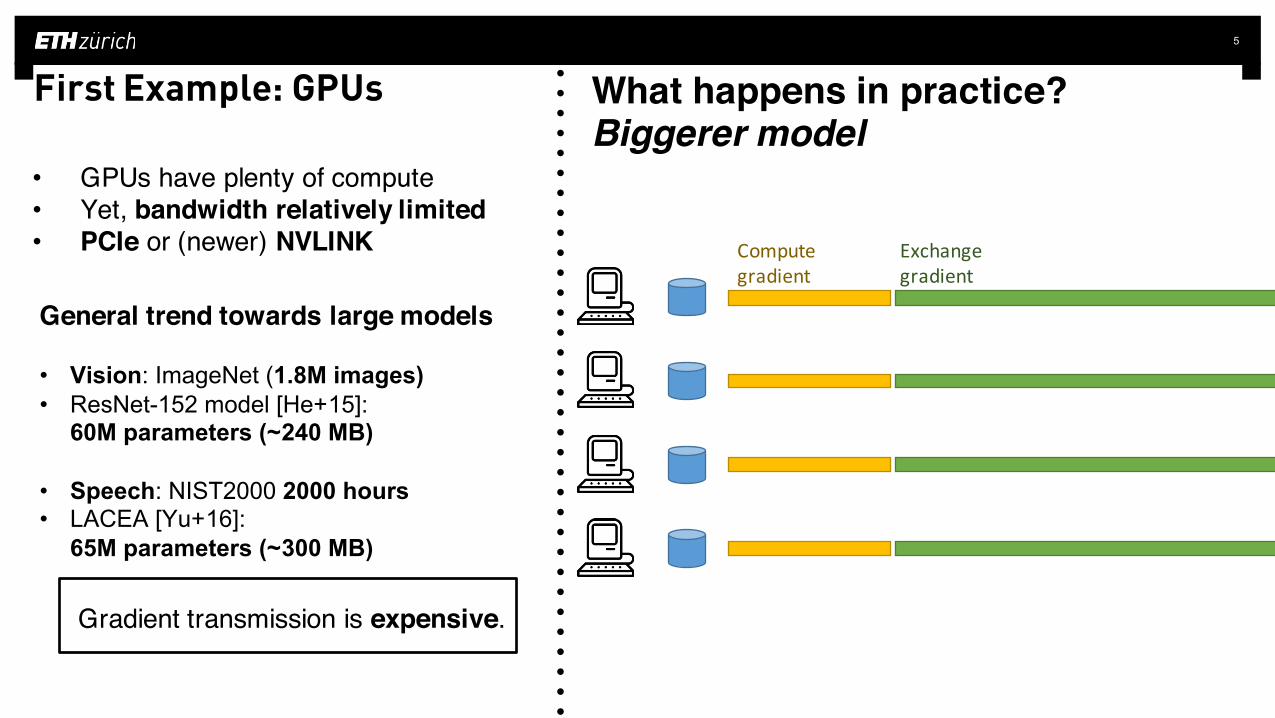
First Example: GPUs What happens in practice?Biggerer model

Computegradient

Exchangegradient

Updateparams

Minibatch 2








6

First Example: GPUs Compression [Seide et al., Microsoft CNTK]

Minibatch 1








The Key Question

Can lossy compression provide speedup, while preserving convergence?

Top-1 accuracy for AlexNet (ImageNet). Top-1 accuracy vs Time for AlexNet (ImageNet).

> 2x faster

Yes. Quantized SGD (QSGD) can converge as fast as SGD, with considerably less bandwidth.

8

Why does QSGD work?

Notation in One Slide

Task

Data (M examples)

argmin𝒙𝑓 𝒙

𝑓 𝑥 =(1/𝑀)0𝑙𝑜𝑠𝑠(𝑥, 𝑒𝑖)7

89:

Notion of “quality”

Solved via optimization procedure.

E.g., image classificationModel 𝑥

Background on Stochastic Gradient Descent

▪ Stochastic Gradient Descent:Goal: find argmin𝒙𝑓 𝒙 .Let 𝒈A(𝒙) = 𝒙‘s gradient at a randomly chosen data point.Iteration:

𝒙𝒕D𝟏 = 𝒙𝒕 − 𝜼𝒕𝒈A(𝒙𝒕), where 𝜠[𝑔K(𝑥𝑡)] = 𝛻𝑓 𝑥𝑡 .

Theorem [Informal]: Given 𝑓 nice (e.g., convex and smooth), and 𝑅2 = ||𝑥0 − 𝑥∗||2. To converge within 𝜺 of optimal it is sufficient to run for

𝑻 = 𝓞(𝑹𝟐 𝟐𝝈𝟐

𝜺𝟐) iterations.

Let 𝜠 𝒈A 𝒙 − 𝜵𝒇 𝒙 𝟐 ≤ 𝝈𝟐 (variance bound)

Higher variance = more iterations to convergence.

11

Data Flow: Data-Parallel Training (e.g. GPUs)

GPU 1 GPU 2

Data Data

Model 𝒙𝒕

𝒙𝒕D𝟏 = 𝒙𝒕 − 𝜼𝒕𝜵𝒈A 𝒙𝒕 at step t.

𝜵𝒈𝟏] 𝒙𝒕 𝜵𝒈𝟐] 𝒙𝒕

Model 𝒙𝒕D𝟏 = 𝒙𝒕 − 𝜼𝒕(𝜵𝒈𝟏] 𝒙𝒕 + 𝜵𝒈𝟐] 𝒙𝒕 )

𝒙𝒕D𝟏 = 𝒙𝒕 − 𝜼𝒕𝑸(𝜵𝒈A 𝒙𝒕 ) at step t.

Standard SGD step:

Quantized SGD step:

𝑸() 𝑸()-5 -4 -3 -2 -1 0 1 2 3 4 50

2000

4000

6000

8000

10000

12000

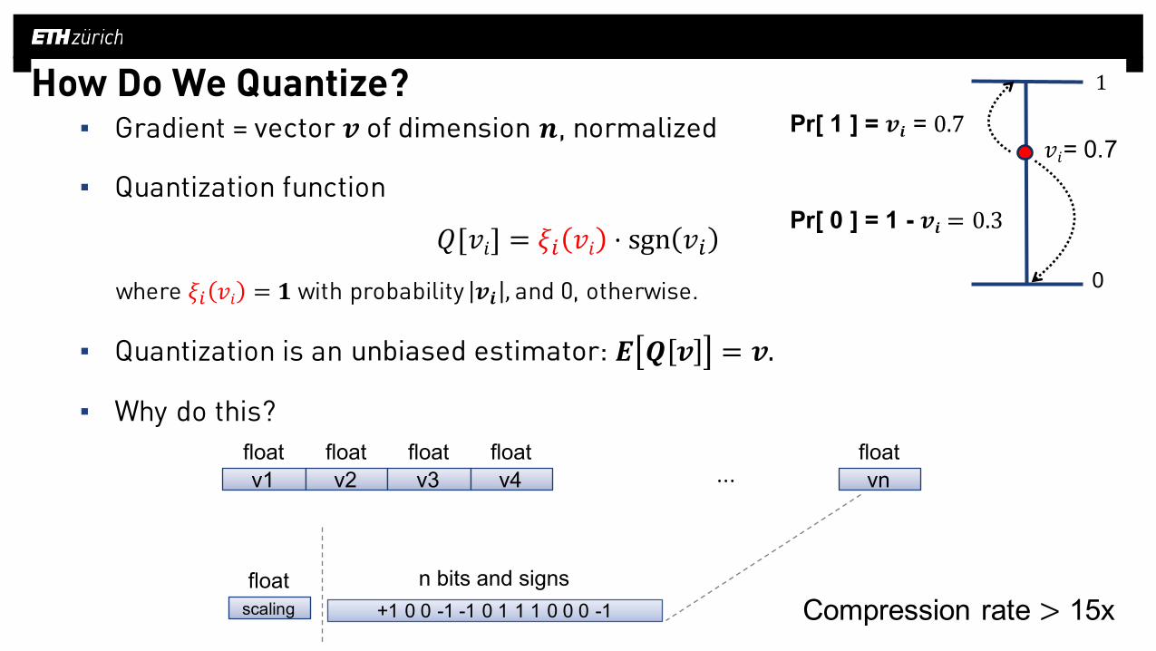
How Do We Quantize?▪ Gradient = vector 𝒗 of dimension 𝒏, normalized

▪ Quantization function

𝑄[𝑣𝑖] = 𝜉8 𝑣𝑖 ⋅ sgn 𝑣8where 𝜉8 𝑣𝑖 = 𝟏 with probability 𝒗𝒊 ,and 0, otherwise.

▪ Quantization is an unbiased estimator: 𝑬 𝑸 𝒗 = 𝒗.

▪ Why do this?

0

1

𝑣𝑖= 0.7

v1float

v2float

v3float

v4float

vnfloat

⋯

scalingfloat

+1 0 0 -1 -1 0 1 1 1 0 0 0 -1 Compression rate > 15xn bits and signs

Pr[ 1 ] = 𝒗𝒊 = 0.7

Pr[ 0 ] = 1 - 𝒗𝒊 = 0.3

13

Gradient Compression

0

1

0.143

0.286

0.429

0.571

0.714

0.857

• We apply stochastic rounding to gradients• The SGD iteration becomes:

𝒙𝒕D𝟏 = 𝒙𝒕 − 𝜼𝒕𝑸(𝒈A 𝒙𝒕 ) at step t.

Theorem [QSGD: Alistarh, Grubic, Li, Tomioka, Vojnovic, 2016]Given dimension n, QSGD guarantees the following:

1. Convergence:If SGD converges, then QSGD converges.

2. Convergence speed:If SGD converges in T iterations, QSGD converges in ≤ 𝒏� T iterations.

3. Bandwidth cost: Each gradient can be coded using ≤ 𝟐 𝒏� log𝒏 bits.

Generalizes to arbitrarily many quantization levels.

The Gamble: The benefit of reduced communication will outweigh the performance hit because of extra iterations/variance and coding/decoding.

14

Does it actually work?

Experimental Setup

Where?▪ Amazon p16xLarge (16 x NVIDIA K80 GPUs)▪ Microsoft CNTK v2.0, with MPI-based communication (no NVIDIA NCCL)What?▪ Tasks: image classification (ImageNet) and speech recognition (CMU AN4)▪ Nets: ResNet, VGG, Inception, AlexNet, respectively LSTM▪ With default parametersWhy?▪ Accuracy vs. Speed/Scalability

Open-source implementation, as well as docker containers.

▪ AlexNet x ImageNet-1K x 2 GPUs

Experiments: Communication Cost

SGD vs QSGD on AlexNet.

Compute

Communicate

60%

40%Compute 95%

5%Communicate

Experiments: “Strong” Scaling

2.3x3.5x

1.6x 1.3x

Experiments: A Closer Look at Accuracy

3-Layer LSTM on CMU AN4 (Speech)

2.5x

ResNet50 on ImageNet

Across all networks we tried, 4 bits are sufficient for full accuracy. (QSGD arxiv tech report contains full numbers and comparisons.)

4bit: - 0.2%8bit: + 0.3%

19

How many bits do you need to representa single number in machine learning systems?

0

4

8

1 10 100


3bit



20

Data Flow in Machine Learning Systems

Data SourceSensor

Database

ComputationDevice

GPU, CPUFPGA

Storage DeviceDRAMCPU Cache

Data Ar Model x

Gradient: dot(Ar, x)Ar

1 2

3

21

ZipML

Data SourceSensor

Database

ComputationDeviceFPGA

GPU, CPU


Data Ar Model x


1 2

3

[…. 0.7 ….]

Expectation matches=> OK!

(Over-simplified, need to be careful about variance!)

NIPS’15

0

1 Naive solution: nearest rounding (=1)=> Converge to a different solution

Stochastic rounding: 0 with prob 0.3, 1 with prob 0.7

22

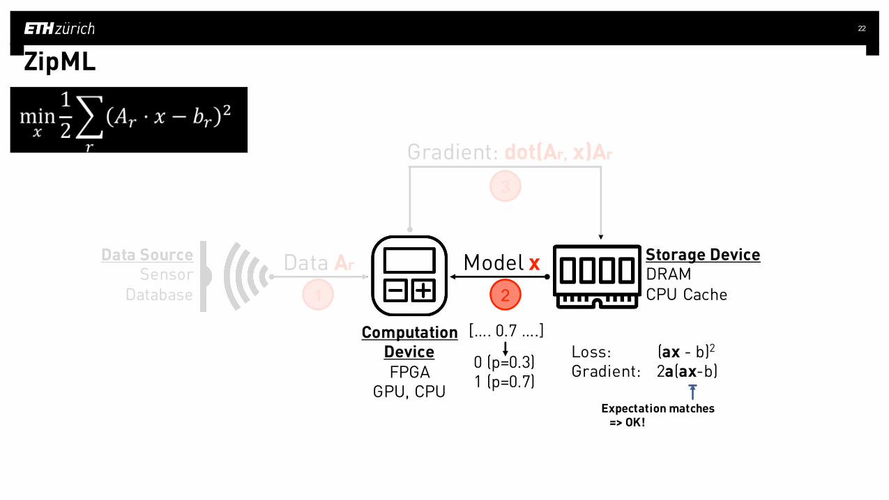
ZipML

Data SourceSensor

Database


GPU, CPU


Data Ar Model x


1 2

3

[…. 0.7 ….]

0 (p=0.3)1 (p=0.7)

Expectation matches=> OK!

Loss: (ax - b)2

Gradient: 2a(ax-b)

23

ZipML

Data SourceSensor

Database


GPU, CPU


Data Ar Model x


1 2

3

[…. 0.7 ….]

0 (p=0.3)1 (p=0.7)

Expectation matches=> OK?

NO!!Why? Gradient 2a(ax-b) is not linear in a.

24

ZipML: “Double Sampling”

How to generate samples for a to getan unbiased estimator for 2a(ax-b)?

arXiv’16

TWO Independent

Samples!

2a1(a2x-b)

FirstSample

SecondSample

How many more bits do we need to store the second sample?

Not 2x Overhead!

3bits to store the first sample

2nd sample only have 3 choices:- up, down, same

We can do even better—Samples are symmetric!

15 different possibilities

=> 4bits to store 2 samples

1bit Overhead

=> 2bits to store

25

It works!

26

Experiments 32bit Floating Points

12bit Fixed Points

Tomographic Reconstruction

Linear regression with fancy regularization (but a 240GB model)

28

It works, but is what we are doing optimal?

Not Really

29

Intuitively, shouldn’twe put moremarkers here?

Data-optimal Quantization Strategy

a bProbability of quantizing to A: PA = b / (a+b)Probability of quantizing to B: PB = a / (a+b)

Expectation of quantization error for A, B (variance)= a PA + b PB = 2ab / (a+b)

Not Really

30

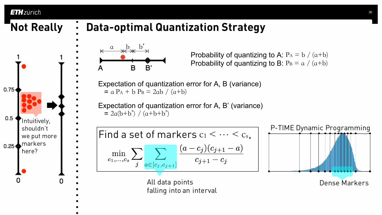
Intuitively, shouldn’twe put moremarkers here?

Data-optimal Quantization Strategy

Probability of quantizing to A: PA = b / (a+b)Probability of quantizing to B: PB = a / (a+b)

Expectation of quantization error for A, B’ (variance)= 2a(b+b’) / (a+b+b’)

b’

Find a set of markers c1 < … < cs,

All data points falling into an interval

P-TIME Dynamic Programming

Dense Markers

a b

Expectation of quantization error for A, B (variance)= a PA + b PB = 2ab / (a+b)

Experiments

31

32

Beyond Linear Regression

33

General Loss Function

Linear Regression or LS-SVM

Logistic Regression

Challenge: Non-Linear terms

Approximationvia polynomials

Chebyshev Polynomials

Experiments 34

Even for non-linear models, we can do end-to-endquantization at 8 bits, with guaranteed convergence.

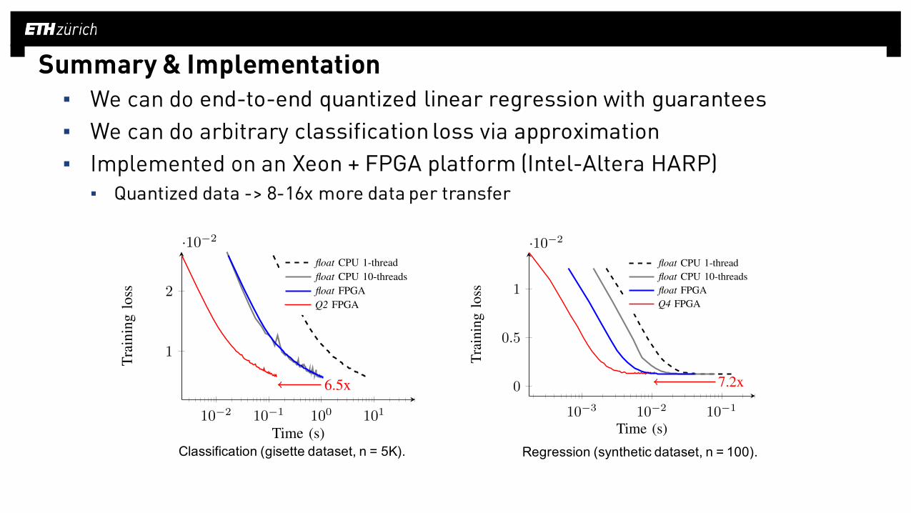
Summary & Implementation▪ We can do end-to-end quantized linear regression with guarantees▪ We can do arbitrary classification loss via approximation▪ Implemented on an Xeon + FPGA platform (Intel-Altera HARP)

▪ Quantized data -> 8-16x more data per transfer

10

�2

10

�1

10

0

10

1

1

2

·10�2

6.5x

float CPU 1-threadfloat CPU 10-threadsfloat FPGAQ2 FPGA

Time (s)

Trai

ning

loss

(a) gisette. � = 1/212.

10

�2

10

�1

10

0

0.04

0.06

0.08

0.1

3.6x


Time (s)Tr

aini

nglo

ss(b) epsilon. � = 1/212.

10

�2

10

�1

10

0

10

1

1.8

2

2.2·10�2

10.6x

float CPU 1-threadfloat CPU 10-threadfloat FPGAQ1 FPGA

Time (s)

Trai

ning

loss

(c) mnist, trained for digit 7. � = 1/215.

Fig. 5: SGD on classification data. All curves represent 64 SGD epochs. Speedup shown for Qx FPGA vs. float CPU 10-threads.

10

�3

10

�2

10

�1

1

1.5

2

2.5

·10�2

3.7x


Time (s)

Trai

ning

loss

(a) cadata. � = 1/212.

10

�3

10

�2

10

�1

0

0.5

1

·10�2

7.2x


Time (s)

Trai

ning

loss

(b) synthetic100. � = 1/29.

10

�2

10

�1

10

0

0

1

2

·10�2

2x


Time (s)Tr

aini

nglo

ss(c) synthetic1000. � = 1/29.

Fig. 6: SGD on regression data. All curves represent 64 SGD epochs. Speedup shown for Qx FPGA vs. float CPU 10-threads.

TABLE IV: Data sets used in experimental evaluation.

Name Training size Testing size # Features # Classescadata 20,640 8 regressionmusic 463,715 90 regression

synthetic100 10,000 100 regressionsynthetic1000 10,000 1000 regression

mnist 60,000 10,000 780 10gisette 6000 1000 5000 2epsilon 10,000 10,000 2000 2

updates; that is, each thread works on a separate chunk of dataand applies gradient updates to a common model without anysynchronization. Although this results in convergence speedupfor sparse data sets, for dense and high variance ones theconvergence quality might be affected negatively, becauseof the lack of synchronization. hogwild also makes use ofvectorization, benefiting from AVX extensions.

Methodology: Since we apply the step size as a bit-shiftoperation, we choose one of the following step sizes, whichresults in the smallest loss for the full-precision data after64 epochs: (1/26, 1/29, 1/212, 1/215). With a determinedconstant step size, we run FPGA-SGD on all the precisionvariations that we have implemented (Q1-only for classifica-tion data-, Q2, Q4, Q8, float). For each data set, we present theloss function over time in Figures 6-5, which always containsingle-threaded and 10-threaded CPU-SGD curve for float, anFPGA-SGD curve for float (for supported dimensions) and anFPGA-SGD curve for the smallest precision data, that hasconverged within 5% of the original loss. We would like toshow the difference in time for all implementations to convergeto the same loss, emphasizing the speedup we can achieve withquantized FPGA-SGD to full precision variants.

Main results: In Figure 5 we can observe that for all classi-fication data sets the quantized FPGA-SGD achieves speedupwhile maintaining convergence quality. For gisette in Figure5a, Q2 reaches the same loss 6.9x faster than hogwild. Dueto high variance data in epsilon, both hogwild and Qx curvesseem to be shaky, in Figure 5b. We can see that float FPGA-SGD in this case behaves very nicely, providing both 1.8xspeedup over hogwild and better convergence quality. Theresults for the music data set are very similar to epsilon, sowe omit showing them for space constraints. On mnist dataset in Figure 5c, we can even use Q1 without losing anyconvergence quality, showing that the characteristics of thedata set effect the choice of quantization precision heavily,which justifies having multiple Qx implementations. For thisone, Q1 FPGA-SGD provides 10.6x speedup over hogwild and11x speedup over float FPGA-SGD. In Figure 6a we see thatfloat FPGA-SGD converges as fast as Q2. The reason for thatis the zero padding we apply to be cache-line aligned (seeSection III): The cadata data set has only 8 features, meaninga full row fits into one cache-line (64B, can contain 16 floats)even if data is in float. Quantizing the data there does notbring any benefits for out implementation, since we pad theremaining bits in a cache-line with zeros. The outcome ofthis experiment, as predicted by our calculations previously, isthat for data sets with a small number of features, quantizationdoes not provide speedup. For synthetic100 and synthetic1000,we need to use Q4 and Q8, respectively, to achieve the sameconvergence quality as float. We see in Figure 6c that hogwildconvergence is slightly faster than the float FPGA-SGD, butthen Q8 provides 2x speedup over that. The reason for hogwild

Classification (gisette dataset, n = 5K).

10

�2

10

�1

10

0

10

1

1

2

·10�2

6.5x


Time (s)

Trai

ning

loss

(a) gisette. � = 1/212.

10

�2

10

�1

10

0

0.04

0.06

0.08

0.1

3.6x


Time (s)

Trai

ning

loss

(b) epsilon. � = 1/212.

10

�2

10

�1

10

0

10

1

1.8

2

2.2·10�2

10.6x

float CPU 1-threadfloat CPU 10-threadfloat FPGAQ1 FPGA

Time (s)

Trai

ning

loss

(c) mnist, trained for digit 7. � = 1/215.

Fig. 5: SGD on classification data. All curves represent 64 SGD epochs. Speedup shown for Qx FPGA vs. float CPU 10-threads.

10

�3

10

�2

10

�1

1

1.5

2

2.5

·10�2

3.7x


Time (s)

Trai

ning

loss

(a) cadata. � = 1/212.

10

�3

10

�2

10

�1

0

0.5

1

·10�2

7.2x


Time (s)

Trai

ning

loss

(b) synthetic100. � = 1/29.

10

�2

10

�1

10

0

0

1

2

·10�2

2x


Time (s)

Trai

ning

loss

(c) synthetic1000. � = 1/29.

Fig. 6: SGD on regression data. All curves represent 64 SGD epochs. Speedup shown for Qx FPGA vs. float CPU 10-threads.

TABLE IV: Data sets used in experimental evaluation.

Name Training size Testing size # Features # Classescadata 20,640 8 regressionmusic 463,715 90 regression

synthetic100 10,000 100 regressionsynthetic1000 10,000 1000 regression

mnist 60,000 10,000 780 10gisette 6000 1000 5000 2epsilon 10,000 10,000 2000 2

updates; that is, each thread works on a separate chunk of dataand applies gradient updates to a common model without anysynchronization. Although this results in convergence speedupfor sparse data sets, for dense and high variance ones theconvergence quality might be affected negatively, becauseof the lack of synchronization. hogwild also makes use ofvectorization, benefiting from AVX extensions.

Methodology: Since we apply the step size as a bit-shiftoperation, we choose one of the following step sizes, whichresults in the smallest loss for the full-precision data after64 epochs: (1/26, 1/29, 1/212, 1/215). With a determinedconstant step size, we run FPGA-SGD on all the precisionvariations that we have implemented (Q1-only for classifica-tion data-, Q2, Q4, Q8, float). For each data set, we present theloss function over time in Figures 6-5, which always containsingle-threaded and 10-threaded CPU-SGD curve for float, anFPGA-SGD curve for float (for supported dimensions) and anFPGA-SGD curve for the smallest precision data, that hasconverged within 5% of the original loss. We would like toshow the difference in time for all implementations to convergeto the same loss, emphasizing the speedup we can achieve withquantized FPGA-SGD to full precision variants.

Main results: In Figure 5 we can observe that for all classi-fication data sets the quantized FPGA-SGD achieves speedupwhile maintaining convergence quality. For gisette in Figure5a, Q2 reaches the same loss 6.9x faster than hogwild. Dueto high variance data in epsilon, both hogwild and Qx curvesseem to be shaky, in Figure 5b. We can see that float FPGA-SGD in this case behaves very nicely, providing both 1.8xspeedup over hogwild and better convergence quality. Theresults for the music data set are very similar to epsilon, sowe omit showing them for space constraints. On mnist dataset in Figure 5c, we can even use Q1 without losing anyconvergence quality, showing that the characteristics of thedata set effect the choice of quantization precision heavily,which justifies having multiple Qx implementations. For thisone, Q1 FPGA-SGD provides 10.6x speedup over hogwild and11x speedup over float FPGA-SGD. In Figure 6a we see thatfloat FPGA-SGD converges as fast as Q2. The reason for thatis the zero padding we apply to be cache-line aligned (seeSection III): The cadata data set has only 8 features, meaninga full row fits into one cache-line (64B, can contain 16 floats)even if data is in float. Quantizing the data there does notbring any benefits for out implementation, since we pad theremaining bits in a cache-line with zeros. The outcome ofthis experiment, as predicted by our calculations previously, isthat for data sets with a small number of features, quantizationdoes not provide speedup. For synthetic100 and synthetic1000,we need to use Q4 and Q8, respectively, to achieve the sameconvergence quality as float. We see in Figure 6c that hogwildconvergence is slightly faster than the float FPGA-SGD, butthen Q8 provides 2x speedup over that. The reason for hogwild

Regression (synthetic dataset, n = 100).

Questions?

0

4

8

1 10 100


3bit



Beyond EmpiricalRigorous theoretical guarantees

Date post:	05-Apr-2018
Category:	Documents
Upload:	doanliem
View:	217 times
Download:	0 times

Faster Machine Learning via Low-Precision Communication...

Documents